Communication Efficient Distributed Optimization using an Approximate Newton-type Method

Abstract

We present a novel Newton-type method for distributed optimization, which is particularly well suited for stochastic optimization and learning problems. For quadratic objectives, the method enjoys a linear rate of convergence which provably improves with the data size, requiring an essentially constant number of iterations under reasonable assumptions. We provide theoretical and empirical evidence of the advantages of our method compared to other approaches, such as one-shot parameter averaging and ADMM.

1 Introduction

We consider the problem of distributed optimization, where each of $m$ machines has access to a function $\phi_{i}:\mathbb{R}^{d}\rightarrow\mathbb{R}$, $i=1,\ldots,m$, and we would like to minimize their average

$$\phi(w)=\tfrac{1}{m}\sum_{i=1}^{m}\phi_{i}(w).$$ (1)

We are particularly interested in a stochastic optimization (learning) setting, where the ultimate goal is to minimize some stochastic (population) objective (e.g. expected loss or generalization error)

$$F(w)=\operatorname*{\mathbb{E}}_{z\sim\mathcal{D}}[f(w,z)]$$ (2)

and each of the $m$ machines has access to $n$ i.i.d. samples $z_{i}^{1},\ldots,z_{i}^{n}$ from the source distribution $\mathcal{D}$, for a total of $N=nm$ independent samples evenly and randomly distributed among the machines. Each machine $i$ can construct a local empirical (sample) estimate of $F(w)$:

$$\phi_{i}(w)=\hat{F}_{i}(w)=\frac{1}{n}\sum_{j=1}^{n}f(w,z_{i}^{j})$$ (3)

and the overall empirical objective is then:

$$\phi(w)=\hat{F}(w)=\frac{1}{m}\sum_{i=1}^{m}\hat{F}_{i}(w)=\frac{1}{nm}\sum_{i,j}f(w,z_{i}^{j}).$$ (4)

We can then use the empirical risk minimizer (ERM)

$$\hat{w}=\arg\min\hat{F}(w)$$ (5)

as an approximate minimizer of $F(w)$. Since our interest lies mostly with this stochastic optimization setting, we will denote $\hat{w}=\arg\min\phi(w)$ even when the optimization objective $\phi(w)$ is not an empirical approximation to a stochastic objective.

When considering distributed optimization, two resources are at play: the amount of processing on each machine, and the communication between machines. In this paper, we focus on algorithms which alternate between a local optimization procedure at each machine, and a communication round involving simple map-reduce operations such as distributed averaging of vectors in $\mathbb{R}^{d}$. Since the cost of communication is very high in practice (Bekkerman et al., 2011), our goal is to develop methods which quickly optimize the empirical objective $\hat{F}(\cdot)$, using a minimal number of such iterations.

One-Shot Averaging

A straight-forward single-iteration approach is for each machine to optimize its own local objective, obtaining

$$\hat{w}_{i}=\arg\min\phi_{i}(w),$$ (6)

and then to compute their average:

$$\bar{w}=\frac{1}{m}\sum_{i=1}^{m}\hat{w}_{i}.$$ (7)

This approach, which we refer to as “one-shot parameter averaging”, was recently considered in Zinkevich et al. (2010) and further analyzed by Zhang et al. (2013). The latter also proposed a bias-corrected improvement which perturbs each $\hat{w}_{i}$ using the optimum on a bootstrap sample. This approach gives only an approximate minimizer of $\phi(w)$ with some finite suboptimality, rather then allowing us converge to $\hat{w}$ (i.e. to obtain solutions with any desired suboptimality $\epsilon$). Although approximate solutions are often sufficient for stochastic optimization, we prove in Section 2 that the one-shot solution $\bar{w}$ can be much worse in terms of minimizing the population objective $F(w)$, compared to the actual empirical minimizer $\hat{w}$. It does not seem possible to address this suboptimality by more clever averaging, and instead additional rounds of communications appear necessary.

Gradient Descent

One possible multi-round approach to distributed optimization is a distributed implementation of gradient descent: at each iteration each machine calculates $\nabla\phi_{i}(w^{(t)})$ at the current iterate $w^{(t)}$, and then these are averaged to obtain the overall gradient $\nabla\phi(w^{(t)})$, and a gradient step is taken. As the iterates are then standard gradient descent iterates, the number of iterations, and so also number of communication rounds, is linear in the conditioning of the problem – or, if accelerated gradient descent is used, proportional to the square root of the condition number: If $\phi(w)$ is $L$-smooth and $\lambda$-strongly convex, then

$$\mathcal{O}\left(\sqrt{\frac{L}{\lambda}}\log\left(\frac{1}{\epsilon}\right)\right)$$ (8)

iterations are needed to attain an $\epsilon$-suboptimal solution. The polynomial dependence on the condition number may be disappointing, as in many problems the parameter of strong convexity $\lambda$ might be very small. E.g., when strong convexity arises from regularization, as in many stochastic optimization problems, $\lambda$ decreases with the overall sample size $N=nm$, and is typically at most $1/\sqrt{nm}$ (Sridharan et al. 2008; Shalev-Shwartz et al. 2009; and see also Section 4.3 below). The number of iterations / communication rounds needed for distributed accelerated gradient descent then scales as $\sqrt[4]{nm}$, i.e. increases polynomially with the sample size.

Instead of gradient descent, one may also consider more sophisticated methods which utilize gradient information, such as quasi-Newton methods. For example, a distributed implementation using L-BFGS has been proposed in Agarwal et al. (2011). However, no guarantee better then (8) can be ensured for gradient-based methods Nemirovsky and Yudin (1983), and we thus may still get a polynomial dependence on the sample size.

ADMM and other approaches

Another popular approach is distributed alternating direction method of multipliers (ADMM, e.g. Boyd et al. 2011), where the machines alternate between computing shared dual variables in a distributed manner, and solving augmented Lagrangian problems with respect to their local data. However, the convergence of ADMM can be slow. Although recent works proved a linear convergence rate under favorable assumptions Deng and Yin (2012); Hong and Luo (2012), we are not aware of any analysis where the number of iterations / communication rounds doesn’t scale strongly with the condition number, and hence the sample size, for learning applications. A similar dependence occurs with other recently-proposed algorithms for distributed optimization (e.g. Yang, 2013; Mahajan et al., 2013; Dekel et al., 2012; Cotter et al., 2011; Duchi et al., 2012). We also mention that our framework is orthogonal to much recent work on distributed coordinate descent methods (e.g. Recht et al., 2011; Richtárik and Takác, 2013), which assume the data is split feature-wise rather than instance-wise.

Our Method

The method we propose can be viewed as an approximate Newton-like method, where at each iteration, instead of a gradient step, we take a step appropriate for the geometry of the problem, as estimated on each machine separately. In particular, for quadratic objectives, the method can be seen as taking approximate Newton steps, where each machine $i$ implicitly uses its local Hessian $\nabla^{2}\phi_{i}(w)$ (although no Hessians are explicitly computed!). Unlike ADMM, our method can take advantage of the fact that for machine learning applications, the sub-problems are usually similar: $\phi_{i}\approx\phi$. We refer to our method as DANE—Distributed Approximate NEwton.

DANE is applicable to any smooth and strongly convex problem. However, as is typical of Newton and Newton-like methods, its generic analysis is not immediately apparent. For general functions, we can show convergence, but cannot rigorously prove improvement over gradient descent. Instead, in order to demonstrate DANE’s advantages and give a sense of its benefits, we focus our theoretical analysis on quadratic objectives. For stochastic quadratic objectives, where $f(w,z)$ is $L$-smooth and $\lambda$-strongly convex in $w\in\mathbb{R}^{d}$, we show that

$$\mathcal{O}\left(\frac{(L/\lambda)^{2}}{n}\log(dm)\log(\frac{1}{\epsilon})\right)$$ (9)

iterations are sufficient for DANE to find $\tilde{w}$ such that with high probability $\hat{F}(\tilde{w})\leq\hat{F}(\hat{w})+\epsilon$. When $L/\lambda$ is fixed and the number of examples $n$ per machine is large (the regime considered by Zhang et al. 2013), (9) establishes convergence after a constant number of iterations / communication rounds. When $\lambda$ scales as $1/\sqrt{nm}$, as discussed above, (9) yields convergence to the empirical minimizer in a number of iterations that scales roughly linearly with the number of machines $m$, but not with the sample size $N=nm$. To the best of our knowledge, this is the first algorithm which provably has such a behavior. We also provide evidence for similar behavior on non-quadratic objectives.

Notation and Definitions

For vectors, $\|v\|$ is always the Euclidean norm, and for matrices $\|A\|_{2}$ is the spectral norm. We use $\lambda\preccurlyeq A\preccurlyeq L$ to indicate that the eigenvalues of $A$ are bounded between $\lambda$ and $L$. We say that a twice differentiable function $f(w)$ is $\lambda$-strongly convex or $L$-smooth, iff for all $w$, its Hessian is bounded from below by $\lambda$ (i.e. $\lambda\preccurlyeq\nabla^{2}f(w)$), or above by $L$ (i.e. $\nabla^{2}f(w)\preccurlyeq L$) respectively.

2 Stochastic Optimization and One-shot Parameter Averaging

In a stochastic optimization setting, where the true objective is the population objective $F(w)$, there is a limit to the accuracy with which we can minimize $F(w)$ given only $N=nm$ samples, even using the exact empirical minimizer $\hat{w}$. It is thus reasonable to compare the suboptimality of $F(w)$ when using the exact $\hat{w}$ to what can be attained using distributed optimization with limited communication.

When $f(w,z)$ has gradients with bounded second moments, namely when $\forall_{w}\operatorname*{\mathbb{E}}_{z}\left[\|\nabla_{w}f(w,z)\|^{2}\right]\leq G^{2}$, and $F(w)$ is $\lambda$-strongly convex, then (Shalev-Shwartz et al., 2009)

$$\operatorname*{\mathbb{E}}[F(\hat{w})]\leq F(w^{*})+\mathcal{O}\left(\frac{G^{2}}{\lambda N}\right)=\inf_{w}F(w)+\mathcal{O}\left(\frac{G^{2}}{\lambda nm}\right)$$ (10)

where $w^{*}=\arg\min F(w)$ is the population minimizer and the expectation is with respect to the random sample of size $N=nm$. One might then ask whether a suboptimality of $\epsilon=\mathcal{O}\left(\frac{G^{2}}{\lambda nm}\right)$ can be also be achieved using a few, perhaps only one, round of communication. This is different from seeking a distributed optimization method that achieves any arbitrarily small empirical suboptimality, and thus converges to $\hat{w}$, but might be sufficient in terms of stochastic optimization.

For one-shot parameter averaging, Zhang et al. (2013, Corollary 2) recently showed that for $\lambda$-strongly convex objectives, and when moments of the first, second and third derivatives of $f(w,z)$ are bounded by $G$, $L$, and $M$ respectively, then

$$\operatorname*{\mathbb{E}}{\|\bar{w}-w^{*}\|^{2}}\leq\tilde{\mathcal{O}}\left(\frac{G^{2}}{\lambda^{2}nm}+\frac{G^{4}M^{2}}{\lambda^{6}n^{2}}+\frac{L^{2}G^{2}\log d}{\lambda^{4}n^{2}}\right),$$ (11)

where $\bar{w}$ is the one-shot average estimator defined in (7). This implies that the population suboptimality $\operatorname*{\mathbb{E}}[F(\bar{w})]-F(w^{*})$ is bounded by

$$\tilde{\mathcal{O}}\left(\frac{LG^{2}}{\lambda^{2}nm}+\frac{LG^{4}M^{2}}{\lambda^{6}n^{2}}+\frac{L^{3}G^{2}\log d}{\lambda^{4}n^{2}}\right).$$ (12)

Zhang et al. (2013) argued that the dependence on the sample size $mn$ above is essentially optimal: the dominant term (as $n\rightarrow\infty$, and in particular when $n\gg m$) scales as $1/(nm)$, which is the same as for the empirical minimizer $\hat{w}$ (as in eq. 10), and so one-shot parameter averaging achieves the same population suboptimality rate, using only a single round of communication, as the best rate we can hope for using unlimited communication, or if all $N=nm$ samples were on the same machine. Moreover, the $\mathcal{O}(n^{-2})$ terms can be replaced by a $\mathcal{O}(n^{-3})$ term using an appropriate bias-correction procedure.

However, this view ignores the dependence on the other parameters, and in particular the strong convexity parameter $\lambda$, which is much worse in (12) relative to (10). The strong convexity parameter often arises from an explicit regularization, and decays as the sample size increases. E.g., in regularized loss minimization and SVM-type problems (Sridharan et al., 2008), as well as more generally for stochastic convex optimization (Shalev-Shwartz et al., 2009), the regularization parameter, and hence the strong convexity parameter, decreases as $\frac{1}{\sqrt{N}}=\frac{1}{\sqrt{nm}}$. In practice, $\lambda$ is often chosen even smaller, possibly as small as $\frac{1}{N}$. Unfortunately, substituting $\lambda=\mathcal{O}(1/\sqrt{nm})$ in (12) results in a useless bound, where even the first term does not decrease with the sample size.

Of course, this strong dependence on $\lambda$ might be an artifact of the analysis of Zhang et al.. However, in Theorem 1 below, we show that even in a simple one-dimensional example, when $\lambda\leq\mathcal{O}(1/\sqrt{n})$, the population sub-optimality of the one-shot estimator (using $m$ machines and a total of $nm$ samples), can be no better then the population sub-optimality using just $n$ samples, and much worse than what can be attained using $nm$ samples. In other words, one-shot averaging does not give any benefit over using only the data on a single machine, and ignoring all other $(m-1)n$ data points.

Theorem 1.

For any per-machine sample size $n\geq 9$, and any $\lambda\in\left(0,\frac{1}{9\sqrt{n}}\right)$, there exists a distribution $\mathcal{D}$ over examples and a stochastic optimization problem on a convex set $\mathcal{W}\subset\mathbb{R}$, such that:

• $f(w;z)$ is $\lambda$-strongly convex, infinitely differentiable, and $\forall_{w\in\mathcal{W}}\operatorname*{\mathbb{E}}_{z}[\|\nabla f(w;z)\|^{2}]\leq 9$.

• For any number of machines $m$, if we run one-shot parameter averaging to compute $\bar{w}$, it holds for some universal constants $C_{1},C_{2},C_{3},C_{4}$ that

  $$\operatorname*{\mathbb{E}}[\|\bar{w}-w^{*}\|^{2}]\geq\frac{C_{1}}{\lambda^{2}n}~{},~{}\operatorname*{\mathbb{E}}[\|\hat{w}-w^{*}\|^{2}]\leq\frac{C_{2}}{\lambda^{2}nm}$$

  $$\operatorname*{\mathbb{E}}[F(\bar{w})]-F(w^{*})\geq\frac{C_{3}}{\lambda n}~{},~{}\operatorname*{\mathbb{E}}[F(\hat{w})]-F(w^{*})\leq\frac{C_{4}}{\lambda nm}$$

The intuition behind the construction of Theorem 1 is that when $\lambda$ is small, the deviation of each machine output $\hat{w}_{i}$ from $w^{*}$ is large, and its expectation is biased away from $w^{*}$. The exact bias amount is highly problem-dependent, and cannot be eliminated by any fixed averaging scheme. Since bias is not reduced by averaging, the optimization error does not scale down with the number of machines $m$. The full construction and proof appear in appendix A. In the appendix we also show that the bias correction proposed by Zhang et al. to reduce the lower-order terms in equation (11) does not remedy this problem.

3 Distributed Approximate Newton-type Method

We now describe a new iterative method for distributed optimization. The method performs two distributed averaging computations per iteration, and outputs a predictor $w^{(t)}$ which, under suitable parameter choices, converges to the optimum $\hat{w}$. The method, which we refer to as DANE (Distributed Approximate NEwton-type Method) is described in Figure 1.

Procedure DANE Parameter: learning rate $\eta>0$ and regularizer $\mu>0$ Initialize: Start at some $w^{(0)}$, e.g. $w^{(0)}=0$ Iterate: for $t=1,2,\dots$ Compute $\nabla\phi(w^{(t-1)})=\frac{1}{m}\sum_{i=1}^{m}\nabla\phi_{i}(w^{(t-1)})$ and distribute to all machines For each machine $i$, solve $w_{i}^{(t)}=\arg\min_{w}\left[\phi_{i}(w)-(\nabla\phi_{i}(w^{(t-1)})-\eta\nabla\phi(w^{(t-1)}))^{\top}w+\frac{\mu}{2}\|w-w^{(t-1)}\|_{2}^{2}\right]$ Compute $w^{(t)}=\frac{1}{m}\sum_{i=1}^{m}w_{i}^{(t)}$ and distribute to all machines             $(*)$ end

Figure 1: Distributed Approximate NEwton-type method (DANE)

DANE maintains an agreed-upon iterate $w^{(t)}$, which is synchronized among all machines at the end of each iteration. In each iteration, we first compute the gradient $\nabla\phi(w^{(t-1)})$ at the current iterate, by averaging the local gradients $\nabla\phi_{i}(w^{(t-1)})$. Each machine then performs a separate local optimization, based on its own local objective $\phi_{i}(w)$ and the computed global gradient $\nabla\phi(w^{(t)})$, to obtain a local iterate $w_{i}^{(t)}$. These local iterates are averaged to obtain the centralized iterate $w^{(t)}$.

The crux of the method is the local optimization performed on each machine at each iteration:

$$w_{i}^{(t)}=\arg\min_{w}[\phi_{i}(w)$$ (13)

$$-(\nabla\phi_{i}(w^{(t-1)})-\eta\nabla\phi(w^{(t-1)}))^{\top}w+\frac{\mu}{2}\|w-w^{(t-1)}\|_{2}^{2}]$$

To understand this local optimization, recall the definition of the Bregman divergence corresponding to a strongly convex function $\psi$:

$$D_{\psi}(w^{\prime};w)=\psi(w^{\prime})-\psi(w)-\langle\nabla\psi(w),w^{\prime}-w\rangle.$$

Now, for each local objective $\phi_{i}$, consider the regularized local objective, defined as

$$h_{i}(w)=\phi_{i}(w)+\frac{\mu}{2}\|w\|^{2}$$

and its corresponding Bregman divergence:

$$D_{i}(w^{\prime};w)=D_{h_{i}}(w^{\prime};w)=D_{\phi_{i}}(w^{\prime};w)+\frac{\mu}{2}\|w^{\prime}-{w}\|^{2}.$$

It is not difficult to check that the local optimization problem (13) can be written as

$$w_{i}^{(t)}=\arg\min_{w}\phi(w^{(t-1)}) +\langle\nabla\phi(w^{(t-1)}),w-w^{(t-1)}\rangle$$

$$+\frac{1}{\eta}D_{i}(w;w^{(t-1)}),$$ (14)

where we also added the terms $\phi(w^{(t-1)})+\langle\nabla\phi(w^{(t-1)}),w^{(t-1)}\rangle$ which do not depend on $w$ and do not affect the optimization. The first two terms in (14) are thus a linear approximation of the overall objective $\phi(w)$ about the current iterate $w^{(t-1)}$, and do not depend on the machine $i$. What varies from machine to machine is the potential function used to localize the linear approximation. The update (14) is in-fact a mirror descent update (Nemirovski and Yudin, 1978; Beck and Teboulle, 2003) using the potential function $h_{i}$, and step size $\eta$.

Let us examine this form of update. When $\mu\rightarrow\infty$ the potential function essentially becomes a squared Euclidean norm, as in gradient descent updates. In fact, when $\eta,\mu\rightarrow\infty$ as $\tilde{\eta}\doteq\frac{\eta}{\mu}$ remains constant, the update (14) becomes a standard gradient descent update on $\phi(w)$ with stepsize $\tilde{\eta}$. In this extreme, the update does not use the local objective $\phi_{i}(w)$, beyond the centralized calculation of $\nabla\phi(w)$, the updates (14) are the same on all machines, and the second round of communication is not needed. DANE reduces to distributed gradient descent, with its iteration complexity of $\mathcal{O}\left(\frac{L}{\lambda}\log(1/\epsilon)\right)$.

At the other extreme, consider the case where $\mu=0$ and all local objectives are equal, i.e. $h_{i}(w)=\phi_{i}(w)=\phi(w)$. Substituting the definition of the Bregman divergence into (14), or simply investigating (13), we can see that $w_{i}^{(t)}=\arg\min\phi_{i}(w)=\arg\min\phi(w)=\hat{w}$. That is, DANE converges in a single iteration to the overall empirical optimum. This is an ideal Newton-type iteration, where the potential function is perfectly aligned with the objective.

Of course, if $\phi_{i}(w)=\phi(w)$ for all machines $i$, we would not need to perform distributed optimization in the first place. Nevertheless, as $n\rightarrow\infty$, we can hope that $\phi_{i}(w)$ are similar enough to each other, such that (14) approximates such an ideal Newton-type iteration, gets us very close to the optimum, and very few such iterations are sufficient.

In particular, consider the case where $\phi_{i}(w)$, and hence also $\phi(w)$ are quadratic. In this case, the Bregman divergence $D_{i}(w;w^{(t-1)})$ takes the form:

$$\frac{1}{2}(w-w^{(t-1)})^{\top}(\nabla^{2}\phi_{i}(w^{(t-1)})+\mu I)(w-w^{(t-1)}),$$ (15)

and the update (14) can be solved in closed form:

$$w_{i}^{(t)} =w^{(t-1)}-\eta(\nabla^{2}\phi_{i}(w^{(t-1)})+\mu I)^{-1}\nabla\phi(w^{(t-1)})$$

$$w^{(t)} =w^{(t-1)}$$

$$-\eta\left(\frac{1}{m}\sum_{i}(\nabla^{2}\phi_{i}(w^{(t-1)})+\mu I)^{-1}\right)\nabla\phi(w^{(t-1)}).$$ (16)

Contrast this with the true Newton update:

$$w^{(t)}=w^{(t-1)}-\eta\left(\frac{1}{m}\sum_{i}\nabla^{2}\phi_{i}(w^{(t-1)})\right)^{-1}\nabla\phi(w^{(t-1)}).$$ (17)

The difference here is that in (16) we approximate the inverse of the average of the local Hessians with the average of the inverse of the Hessians (plus a possible regularizer). Again we see that the DANE update (16) approximates the true Newton update (17), which can be performed in a distributed fashion without communicating the Hessians.

For a quadratic objective, a single Newton update is enough to find the exact optimum. In Section 4 we rigorously analyze the effects of the distributed approximation, and quantify the number of DANE iterations (and thus rounds of communication) required.

For a general convex, but non-quadratic, objective, the standard Newton approach is to use a quadratic approximation to the ideal Bregman divergence $D_{\phi}$. This leads to the familiar quadratic Newton update in terms of the Hessian. DANE uses a different sort of approximation to $D_{\phi}$: we use a non-quadratic approximation, based on the entire objective and not just a local quadratic approximation, but approximate the potential on each node separately. In the stochastic setting, this approximation becomes better and better, and thus the required number of iterations decrease, as $n\rightarrow\infty$.

Since it is notoriously difficult to provide good global analysis for Newton-type methods, we will investigate the global convergence behavior of DANE carefully in the next Section but only for quadratic objective functions. This analysis can also be viewed as indicative for non-quadratic objectives, as locally they can be approximated by quadratics and so should enjoy the same behavior, at least asymptotically. For non-quadratics, we provide a rigorous convergence guarantee when the stepsize $\eta$ is sufficiently small or the regularization parameter $\mu$ is sufficiently large (in Section 5). However, this analysis does not show a benefit over distributed gradient descent for non-quadratics. We partially bridge this gap by showing that even in the non-quadratic case, the convergence rate improves as the local problems $\phi_{i}$ become more similar.

4 DANE for Quadratic Objectives

In this Section, we analyze the performance of DANE on quadratic objectives. We begin in Section 4.1 with an analysis of DANE for arbitrary quadratic objectives $\phi_{i}(w)$, without stochastic assumptions, deriving a guarantee in terms of the approximation error of the true Hessian. Then in Section 4.2 we consider the stochastic setting where the instantaneous objective $f(w,z)$ is quadratic in $w$, utilizing a bound on the approximation error of the Hessian to obtain a performance guarantee for DANE in terms of the smoothness and strong convexity of $f(w,z)$ . In Section 4.3 we also consider the behavior for stochastic optimization problems, where $\lambda$ is set as a function of the sample size $N=nm$.

4.1 Quadratic $\phi_{i}(w)$

We begin by considering the case where each local objective $\phi_{i}(w)$ is quadratic, i.e. has a fixed Hessian. The overall objective $\phi(w)$ is then of course also quadratic.

Theorem 2.

After $t$ iterations of DANE on quadratic objectives with Hessians $H_{i}=\nabla^{2}\phi_{i}(w)$, we have:

$$\|w^{(t)}-\hat{w}\|\leq\|I-\eta\tilde{H}^{-1}H\|_{2}^{t}\|w^{(0)}-\hat{w}\|,$$

where $H=\nabla^{2}\phi(w)=\frac{1}{m}\sum_{i=1}^{m}H_{i}$ and $\tilde{H}^{-1}=\frac{1}{m}\sum_{i=1}^{n}(H_{i}+\mu I)^{-1}$.

The proof appears in Appendix B. The theorem implies that if $\|I-\eta\tilde{H}^{-1}H\|_{2}$ is smaller than $1$, we get a linear convergence rate. Indeed, we would expect $\|I-\eta\tilde{H}^{-1}H\|_{2}\ll 1$ as long as $\eta$ is close to $1$ and $\tilde{H}$ is a good approximation for the true Hessian $H$, hence $\tilde{H}^{-1}H\approx I$. In particular, if $H$ is not too ill-conditioned, and all $H_{i}$ are sufficiently close to their average $H$, we can indeed ensure $\tilde{H}\approx H$. This is captured by the following lemma (whose proof appears in Appendix C):

Lemma 1.

If $0<\lambda\preccurlyeq H\preccurlyeq L$ and for all $i$, $\|H_{i}-H\|_{2}\leq\beta$, then setting $\eta=1$ and $\mu=\max\{0,\frac{8\beta^{2}}{\lambda}-\lambda\}$, we have:

$$\|I-\tilde{H}^{-1}H\|_{2}\leq\begin{cases}\frac{4\beta^{2}}{\lambda^{2}}&\text{if}~{}~{}~{}\frac{4\beta^{2}}{\lambda^{2}}\leq\frac{1}{2}\\ 1-\frac{\lambda^{2}}{16\beta^{2}}&\text{otherwise}.\end{cases}$$

In the next Section, we consider the stochastic setting, where we can obtain bounds for $\|H_{i}-H\|_{2}$ that improve with the sample size, and plug these into Lemma 1 and Theorem 2 to obtain a performance guarantee for DANE.

4.2 Stochastic Quadratic Problems

We now turn to a stochastic quadratic setting, where $\phi_{i}(w)=\hat{F}_{i}(w)$ as in (3), and the instantaneous losses are smooth and strongly convex quadratics. That is, for all $z$, $f(w,z)$ is quadratic in $w$ and $\lambda\preccurlyeq\nabla^{2}_{w}f(w,z)\preccurlyeq L$.

We first use a matrix concentration bound to establish that all Hessians $H_{i}=\nabla^{2}\hat{F}_{i}(w)$ are close to each other, and hence also to their average:

Lemma 2.

If $0\preccurlyeq\nabla^{2}_{w}f(w,z)\preccurlyeq L$ for all $z$, then with probability at least $1-\delta$ over the samples, $\max_{i}\|H_{i}-H\|_{2}\leq\sqrt{\frac{32L^{2}\log(dm/\delta)}{n}}$, where $H_{i}=\nabla^{2}\hat{F}_{i}(w)$ and $H=\nabla^{2}\hat{F}(w)$.

The proof appears in appendix D. Combining Lemma 2, Lemma 1 and Theorem 2, we can conclude:

Theorem 3.

In the stochastic setting, and when the instantaneous losses are quadratic with $\lambda\preccurlyeq\nabla f(w,z)\preccurlyeq L$, then after

$$t=\mathcal{O}\left(\frac{(L/\lambda)^{2}}{n}\log\left(\frac{dm}{\delta}\right)\log\left(\frac{L\|w^{0}-\hat{w}\|^{2}}{\epsilon}\right)\right)$$

iterations of DANE, we have, with probability at least $1-\delta$, that $\hat{F}(w^{(t)})\leq\hat{F}(\hat{w})+\epsilon$.

The proof appears in Appendix E. From the theorem, we see that if the condition number $L/\lambda$ is fixed, then as $n\rightarrow\infty$ the number of required iterations decreases. In fact, for any target sub-optimality $\epsilon$, as long as the sample size is at least logarithmically large, namely $n=\Omega\left((L/\lambda)^{2}\log(dm)\log(\frac{1}{\epsilon})\right)$, we can obtain the desired accuracy after a constant or even a single DANE iteration! This is a mild requirement on the sample size, since $N$ generally increases at least linearly with $1/\epsilon$.

We next turn to discuss the more challenging case where the condition number decays with the sample size.

4.3 Analysis for Regularized Objectives

Consider a stochastic convex optimization scenario where the instantaneous objectives $f(w,z)$ are not strongly convex. For example, this is the case in linear prediction (including linear and kernel classification and regression, support vector machines, etc.), and more generally for generalized linear objectives of the form $f(w,z)=\ell_{z}(\langle w,\Psi(z)\rangle)$. For such generalized linear objectives, the Hessian $\nabla_{w}^{2}f(w,z)$ is rank-$1$, and so certainly not strongly convex, even if $\ell_{z}(\cdot)$ is strongly convex.

Confronted with such non-strongly-convex objectives, a standard approach is to perform empirical minimization on a regularized objective (Shalev-Shwartz et al., 2009). That is, to define the regularized instantaneous objective

$$f_{\lambda}(w,z)=f(w,z)+\frac{\lambda}{2}\|w\|^{2}$$ (18)

and minimize the corresponding empirical objective $\hat{F}_{\lambda}$. The instantaneous objective $f_{\lambda}(w,z)$ of the modified stochastic optimization problem is now $\lambda$-strongly convex. If $f(w,z)$ are $G$-Lipschitz in $w$, then we have (Shalev-Shwartz et al., 2009):

$$F(\hat{w}_{\lambda}) \leq F_{\lambda}(\hat{w}_{\lambda})\leq F_{\lambda}(w_{\lambda}^{*})+\mathcal{O}\left(\frac{G^{2}}{\lambda N}\right)$$

$$=\inf_{w}\left(F(w)+\frac{\lambda}{2}\|w\|^{2}\right)+\mathcal{O}\left(\frac{G^{2}}{\lambda N}\right)$$

$$\leq\inf_{\|w\|\leq B}F(w)+\mathcal{O}\left(\lambda B^{2}+\frac{G^{2}}{\lambda N}\right),$$

where $\hat{w}_{\lambda}=\arg\min\hat{F}_{\lambda}(w)$ and $w_{\lambda}^{*}=\arg\min F_{\lambda}(w)$. The optimal choice of $\lambda$ in the above is $\lambda=\sqrt{\frac{G^{2}}{B^{2}N}}$, where $B$ is a bound on the predictors we would like to compete with, and with this $\lambda$ we get the optimal rate:

$$F(\hat{w}_{\lambda})\leq\inf_{\|w\|\leq B}F(w)+\mathcal{O}\left(\sqrt{\frac{B^{2}G^{2}}{N}}\right).$$ (19)

It is thus instructive to consider the behavior of DANE when $\lambda=\Theta\left(\sqrt{\frac{G^{2}}{B^{2}N}}\right)=\Theta\left(\sqrt{\frac{G^{2}}{B^{2}nm}}\right)$. Plugging this choice of $\lambda$ into Theorem 3, we get that the number of DANE iterations behaves as:

$$\mathcal{O}\left(\frac{L^{2}B^{2}}{G^{2}}\cdot m\cdot\log(dm)\log(1/\epsilon)\right).$$ (20)

That is, unlike distributed gradient descent, or any other relevant method we are aware of, the number of required iterations / communication rounds does not increase with the sample size, and only scales linearly with the number of machines.

5 Convergence Analysis for Non-Quadratic Objectives

As discussed above, it is notoriously difficult to obtain generic global analysis of Newton-type methods. Our main theoretical result in this paper is the analysis for quadratic objectives, which we believe is also instructive for non-quadratics. Nevertheless, we complement this with a convergence analysis for generic objectives.

We therefore return to considering generic convex objectives $\phi_{i}(w)$. We also do not make any stochastic assumptions. We only assume that each $\phi_{i}(w)$ is $L_{i}$-smooth and $\lambda_{i}$ strongly convex, and that the combined objective $\phi(w)$ is $L$-smooth and $\lambda$-strongly convex.

Theorem 4.

Assume that for all $i,w,z$, $\lambda_{i}\preccurlyeq\nabla^{2}\phi_{i}(w)\preccurlyeq L_{i}$ and $\lambda\preccurlyeq\nabla^{2}\phi(w)\preccurlyeq L$. Let

$$\rho=\frac{1}{m}\sum_{i=1}^{m}\left[\frac{1}{\mu+L_{i}}-\frac{\eta L}{2(\mu+\lambda_{i})^{2}}\right]\eta\lambda.$$

If $\rho>0$, then the DANE iterates satisfy $\phi(w^{(t)})-\phi(\hat{w})\leq(1-\rho)^{t}[\phi(w^{(0)})-\phi(\hat{w})].$

The proof appears in Appendix F. The theorem establishes that with any $\mu>0$ and small enough step-size $\eta$, DANE converges to $\hat{w}$. If each $\phi_{i}(w)$ is strongly convex, we can also take $\mu=0$ and sufficiently small $\eta$ and ensure convergence to $\hat{w}$. However, the optimal setting of $\eta$ and $\mu$ above is to take $\mu\rightarrow\infty$ and set $\eta=\mu/L$, in which case $\rho\rightarrow\lambda/L$, and we recover distributed gradient descent, with the familiar gradient descent guarantee.

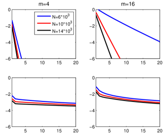
Figure 2: Synthetic dataset: Convergence rate for different number of machines $m$ and sample sizes $N$. The top row presents results for DANE, and the bottom row for ADMM. The $x$-axis is the iteration number, and the $y$-axis is the logarithm (in base 10) of the suboptimality.

We again emphasize that the analysis above is weak and does not take into account the relationship between the local objectives $\phi_{i}(w)$. We believe that the quadratic analysis of Section 4 better captures the true behavior of DANE. Moreover, we can partially bridge this gap by the following result, which shows that a variant of DANE enjoys a linear convergence rate which improves as the local objectives $\phi_{i}$ become more similar to $\phi$ (the proof is in Appendix G):

Theorem 5.

Assume that in the DANE procedure, we replace step $(*)$ by $w^{(t)}=w_{1}^{(t)}$, and define $h(\cdot)=h_{1}(\cdot)$. If there exists $\gamma>0$ such that $\forall w,w^{\prime}$, we have $\gamma D_{h}(w;w^{\prime})\leq D_{\phi}(w;w^{\prime})\leq\eta^{-1}D_{h}(w;w^{\prime})$, then

$$D_{h}(\hat{w};w^{(t)})\leq(1-\eta\gamma)^{t}D_{h}(\hat{w};w^{(0)}).$$

If $\mu$ is small and $\phi_{i}\approx\phi$, then we expect $\gamma\approx 1$ and $\eta\approx 1$. In this case, $\eta\gamma\approx 1$, leading to fast convergence.

6 Experiments

	COV1						ASTRO						MNIST-47
$m$	2	4	8	16	32	64	2	4	8	16	32	64	2	4	8	16	32	64
$\mu=0$	2	2	2	2	2	3	6	6	6	6	12	*	5	5	5	5	6	*
$\mu=3\lambda$	9	9	9	9	9	9	14	14	14	14	14	14	10	10	10	10	10	10
ADMM	3	3	5	9	16	31	24	20	16	16	14	20	23	23	27	21	31	28

Figure 3: Number of iterations required to reach $<10^{-6}$ accuracy on 3 datasets, for varying number of machines $m$. Results are for DANE using $\eta=1$ and $\mu=0,\lambda,3\lambda$, and for ADMM. * Indicates non-convergence after $100$ iterations.

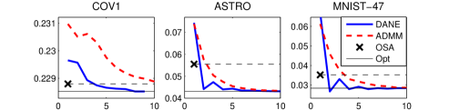
Figure 4: Average regularized smooth-hinge loss on the test set as a function of the iteration number. OSA represents bias-corrected one-shot parameter averaging, which requires a single iteration. ‘Opt’ is the average loss of the exact regularized loss minimizer.

In this section, we present preliminary experimental results on our proposed method. In terms of tuning $\eta,\mu$, we discovered that simply picking $\eta=1,\mu=0$ (which makes DANE closest to a Newton-type iteration, as discussed in Section 3) often results in the fastest convergence. However, in unfavorable situations (such as when the data size per machine is very small), this can also lead to non-convergence. In those cases, convergence can be recovered by slightly increasing $\mu$ to a small positive number. In the experiments, we considered $\mu=0,3\lambda$. These are considerably smaller than what our theory indicates, and we leave the question of the best parameter choice to future research.

We begin by considering a simple quadratic problem using a synthetic dataset, where all parameters can be explicitly controlled. We generated $N$ i.i.d. training examples $(x,y)$ according to the model $y=\langle x,w^{*}\rangle+\xi~{},~{}x\sim\mathcal{N}(0,\Sigma),\xi\sim\mathcal{N}(0,1)$, where $x\in\mathbb{R}^{500}$, the covariance matrix $\Sigma$ is diagonal with $\Sigma_{i,i}=i^{-1.2}$, and $w^{*}$ is the all-ones vector. Given a set of examples $\{x,y\}$ which is assumed to be randomly split to different machines, we then solved a standard ridge regression problem of the form $\min_{w}\frac{1}{N}\sum_{i=1}^{N}(\langle x,w\rangle-y)^{2}+0.005w^{2}$, using DANE (with $\eta=1,\mu=0$). Figure 2 shows the convergence behavior of the algorithm for different number of machines $m$ as the total number of examples $N$ (and hence also the data size per machine) increases. For comparison, we also implemented distributed ADMM Boyd et al. (2011), which is a standard method for distributed optimization but does not take advantage of the statistical similarity between problems at different machines. The results for DANE clearly indicate a linear convergence rate, and moreover, that the rate of convergence improves with the data size, as predicted by our analysis. In contrast, while more data improves the ADMM accuracy after a fixed number of iterations, the convergence rate is slower and does not improve with the data size.

We now turn to present results for solving a smooth non-quadratic problem, this time using non-synthetic datasets. Specifically, we solved a regularized loss minimization problem of the form $\min_{w}\frac{1}{N}\sum_{i=1}^{N}\ell(y_{i}\langle x_{i},w\rangle)+\frac{\lambda}{2}\|w\|^{2},$ where $\ell$ is the smooth hinge loss (as in Shalev-Shwartz and Zhang (2013)) and the training examples $\{(x_{i},y_{i})\}$ are randomly split among different machines. We experimented on $3$ datasets: COV1 and ASTRO-PH (as used in e.g. Shalev-Shwartz and Zhang (2013); Rakhlin et al. (2012)), as well as a subset of the MNIST digit recognition dataset which focuses on discriminating the 4 from the 7 digits. In figure 3, we present the number of iterations required for DANE to reach accuracy $<10^{-6}$ for $\eta=1$ and $\mu=0,3\lambda$, and for different number of machines. We also report results for ADMM on the same datasets. As in the synthetic case, DANE explicitly takes advantage of the similarity between problems on different machines, and we indeed observe that it tends to converge in less iterations than ADMM. Finally, note that for $\mu=0$ and many machines (i.e. few data points per machine), DANE may not converge, and increasing $\mu$ fixes this at the cost of slowing down the average convergence rate.

Finally, we examine the convergence on these datasets in terms of the average loss on the test set. In figure 4, we present the results for $m=64$ machines on the three datasets, using DANE (with $\mu=3\lambda$) and ADMM. We also present for comparison the objective value obtained using one-shot parameter averaging (OSA), using bias correction as proposed in Zhang et al. (2013). The figure highlights the practical importance of multi-round communication algorithms: while DANE and ADMM converge to the value achieved by the regularized loss minimizer, the single-round OSA algorithm may return a significantly suboptimal result.

Acknowledgements:

Ohad Shamir and Nathan Srebro are supported by the Intel ICRI-CI Institute. Ohad Shamir is further supported by an Israel Science Foundation grant 425/13 and an FP7 Marie Curie CIG grant.

Appendix A Lower Bounds for One-shot Parameter Averaging

A.1 Proof of Theorem 1

Before providing the proof details, let us first describe the high-level intuition of our construction. Roughly speaking, one-shot averaging works well when the bias of the predictor returned by each machine (as a random vector in Euclidean space, based on the sampled training data) is much smaller than the variance. Since each such predictor is based on independent data, averaging $m$ such predictors reduces the variance by a factor of $m$, leading to good guarantees. However, averaging has no effect on the bias, so this method is ineffectual when the bias dominates the variance. The construction below shows that when the strong convexity parameter is small, this can indeed happen.

More specifically, when the strong convexity parameter is smaller than $\mathcal{O}(1/\sqrt{n})$, the magnitude of the deviations of the (random) predictor returned by each machine does not decay with the sample size $n$. Moreover, its distribution is highly dependent on the data distribution and the shape of $f$, and is biased in general. Below we use one such construction, which we found to be convenient for precise analytic calculations, but the intuition applies much more broadly.

Specifically, let $\mathcal{W}=[-2/\lambda,\log(1/\lambda)]$, and define the loss function $f(w;z)$ as

$$f(w;z)=\lambda\left(\frac{1}{2}w^{2}+\exp(w)\right)-zw.$$

Furthermore, suppose that $z\sim\mathcal{N}(0,1)$, i.e. the examples have a standard Gaussian distribution. Note that this function is $\lambda$-strongly convex, and can be shown to satisfy $\operatorname*{\mathbb{E}}_{z}[f^{\prime}(w;z)^{2}]\leq 9$ for any $w\in\mathcal{W}$.

Let $\hat{w}_{1}$ be the parameter vector returned by the machine $1$ (this is without loss of generality, since all the machines receive examples drawn from the same distribution). The key to the proof is to show that $\hat{w}_{1}$ is strongly biased, namely that $\operatorname*{\mathbb{E}}[\hat{w}_{1}]$ is bounded away from the true optimum $w^{*}$. To compute $\operatorname*{\mathbb{E}}[\hat{w}_{1}]$, note that $\hat{w}_{1}$ minimizes the random function

$$\frac{1}{n}\sum_{i=1}^{n}f(w;z_{i})=\lambda\left(\frac{1}{2}w^{2}+\exp(w)\right)-\frac{\tilde{z}}{\sqrt{n}}w,$$ (21)

where $\tilde{z}=(z_{1}+\ldots+z_{n})/\sqrt{n}$. Note that since $z_{1},\ldots,z_{n}$ are i.i.d. Gaussians, $\tilde{z}$ also has the same Gaussian distribution $\mathcal{N}(0,1)$.

Taking the derivative, equating to zero and slightly manipulating the result, we get that

$$\lambda\sqrt{n}\left(w+\exp(w)\right)=\tilde{z}.$$

The function on the left-hand-side is strictly monotonically increasing, and has a range $[-\infty,\infty]$. Thus, for any $\tilde{z}$, there exists a unique root $w(\tilde{z})$. Moreover, as long as $|\tilde{z}|\leq\sqrt{n}$, it’s easy to verify that $w(\tilde{z})$ is within our domain $\mathcal{W}=[-2/\lambda,\log(1/\lambda)]$, hence $\hat{w}_{1}=w(\tilde{z})$. Therefore, letting $p(\cdot)$ denote the standard gaussian distribution of $\tilde{z}$, we have

$$\operatorname*{\mathbb{E}}[\hat{w}_{1}] =\int_{x=-\sqrt{n}}^{\sqrt{n}}\hat{w}_{1}p(x)dx+\int_{|x|>\sqrt{n}}\hat{w}_{1}p(x)dx\leq\int_{x=-\sqrt{n}}^{\sqrt{n}}w(x)p(x)dx+\frac{2}{\lambda}\Pr(|\tilde{z}|\geq\sqrt{n})$$

$$\leq\int_{x=0}^{\sqrt{n}}\left(w(x)+w(-x)\right)p(x)dx+\frac{2}{\lambda}\sqrt{\frac{1}{n\exp(n)}},$$ (22)

where in the last step we used the symmetry of the distribution of $\tilde{z}$ and a standard Gaussian tail bound.

We now turn to analyze $w(x)+w(-x)$. First, we have by definition

$$w(x)+\exp(w(x))=\frac{x}{\lambda\sqrt{n}}$$ (23)

for all $x$, and therefore

$$w(x)+w(-x)=\left(\frac{x}{\lambda\sqrt{n}}-\exp(w(x))\right)+\left(-\frac{x}{\lambda\sqrt{n}}-\exp(w(-x))\right)\leq-\exp(w(x)).$$ (24)

Therefore, we have $w(x)+w(-x)\leq 0$ for all $x$. More precisely, considering (23) and the fact that its left hand size is monotonic in $w(x)$, it’s easy to verify that for any $x\geq 0$, we have $w(x)\geq\log\left(\frac{x}{\lambda\sqrt{n}}-\log\left(\frac{x}{\lambda\sqrt{n}}\right)\right)$, and $w(-x)\leq-\frac{x}{\lambda\sqrt{n}}$, so using (24),

$$w(x)+w(-x)\leq-\exp(w(x))\leq-\frac{x}{\lambda\sqrt{n}}+\log\left(\frac{x}{\lambda\sqrt{n}}\right).$$

Since $\log(a)<a/2$ for all $a\geq 0$, this expression is at most $-\frac{x}{2\lambda\sqrt{n}}$. Plugging this back into (22), and using the assumption $n\geq 9$, we get that

$$\operatorname*{\mathbb{E}}[\hat{w}_{1}]\leq-\frac{1}{2\lambda\sqrt{n}}\int_{x=0}^{\sqrt{n}}xp(x)dx+\frac{2}{\lambda}\sqrt{\frac{1}{n\exp(n)}}\leq-\frac{1}{2\lambda\sqrt{n}}\int_{x=0}^{\sqrt{9}}xp(x)dx+\frac{2}{\lambda}\sqrt{\frac{1}{n\exp(n)}}.$$

Since $p(x)$ is the standard Gaussian distribution, it can be numerically checked that this is at most

$$-\frac{0.19}{\lambda\sqrt{n}}+\frac{2}{\lambda}\sqrt{\frac{1}{n\exp(n)}}=\frac{1}{\lambda\sqrt{n}}\left(-0.19+2\sqrt{\exp(-n)}\right)\leq-\frac{1}{6\lambda\sqrt{n}}.$$

So, we finally get $\operatorname*{\mathbb{E}}[\hat{w}_{1}]\leq-1/(6\lambda\sqrt{n})$.

Now, we show that this expected value of $\hat{w}_{1}$ is far away from $w^{*}$. $w^{*}$ is not hard to calculate: It satisfies

$$w^{*}+\exp(w^{*})=0,$$

and it can be calculated numerically that $w^{*}=-0.5671..>-3/5$. Moreover, we assume $\lambda\leq 1/(9\sqrt{n})$, so $\lambda\sqrt{n}\leq 1/9$ and thus it can be verified that

$$w^{*}-\operatorname*{\mathbb{E}}[\hat{w}_{1}]>-\frac{3}{5}+\frac{1}{6\lambda\sqrt{n}}\geq\frac{1}{10~{}\lambda\sqrt{n}}.$$

Note that this is always a positive quantity. As a result, using Jensen’s inequality, we get

$$\operatorname*{\mathbb{E}}[(w^{*}-\bar{w})^{2}]\geq(w^{*}-\operatorname*{\mathbb{E}}[\bar{w}])^{2}=(w^{*}-\operatorname*{\mathbb{E}}[\hat{w}_{1}])^{2}\geq\frac{1}{100~{}\lambda^{2}n}.$$

Moreover, by $\lambda$-strong convexity of $f$, we have that

$$\operatorname*{\mathbb{E}}[F(\bar{w})-F(w^{*})]\geq\operatorname*{\mathbb{E}}\left[\frac{\lambda}{2}(\bar{w}-w^{*})^{2}\right]\geq\frac{1}{200~{}\lambda n}.$$

Finally, it is known that by performing empirical risk minimization over all $N=nm$ instances, and using the fact that $\operatorname*{\mathbb{E}}[\|\nabla_{w}f(w,z)\|^{2}]$ is bounded by a constant, we get

$$\operatorname*{\mathbb{E}}[(\hat{w}-w^{*})^{2}]\leq\mathcal{O}\left(\frac{1}{\lambda^{2}nm}\right)$$

(see Zhang et al. (2013)) and

$$\operatorname*{\mathbb{E}}[F(\hat{w})-F(w^{*})]\leq\mathcal{O}\left(\frac{1}{\lambda nm}\right)$$

(see Equation (10)). Combining the four inequalities above gives us the theorem statement.

A.2 Bias Correction Also Fails

In Zhang et al. (2013), which analyzes one-shot parameter averaging, the authors noticed that the analysis fails for small values of $\lambda$, and proposed a modification of the simple averaging scheme, designed to reduce bias issues. Specifically, given a parameter $r\in[0,1]$, each machine subsamples $rn$ examples without replacement from its dataset, and computes the optimum $\hat{w}_{2,k}$ with respect to this subsample. Then, it computes the optimum $\hat{w}_{k,1}$ over the entire dataset, and returns the weighted combination $\hat{w}_{k}=(\hat{w}_{k,1}-r\hat{w}_{k,2})/(1-r)$. Unfortunately, the analysis still results in lower-order terms with bad dependence on $\lambda$, and it’s not difficult to extend our construction from Theorem 1 to show that this bias-corrected version of the algorithm still fails (at least, if $r$ is chosen in a fixed manner).

For simplicity, we will only sketch the derivation for a fixed choice of $\lambda$ given $n$, namely $\lambda=1/10\sqrt{n}$, and for $r=1/2$. Also, we assume for simplicity that $\mathcal{W}=\mathbb{R}$ (to avoid tedious dealings with small Gaussian tails). With this choice, the returned solution becomes $\hat{w}_{k}=2\hat{w}_{k,1}-\hat{w}_{k,2}$. The distribution of $\hat{w}_{k,1}$, using the same derivation as in the proof of the theorem, is determined by

$$\hat{w}_{k,1}+\exp(\hat{w}_{k,1})=\frac{1}{\lambda\sqrt{n}}\tilde{z}=10\tilde{z}$$

where $\tilde{z}$ has a standard Gaussian distribution. As to $\hat{w}_{k,2}$, its distribution is similar to that of $\hat{w}_{k,1}$ with the same choice of $\lambda$ but only half as many points, hence

$$\hat{w}_{k,2}+\exp(\hat{w}_{k,2})=\frac{1}{\lambda\sqrt{n/2}}\tilde{z}=10\sqrt{2}~{}\tilde{z}.$$

By a numerical calculation, one can verify that $\operatorname*{\mathbb{E}}[\hat{w}_{k}]=2\operatorname*{\mathbb{E}}[\hat{w}_{k,1}]-\operatorname*{\mathbb{E}}[\hat{w}_{k,2}]\approx 2*(-3.3)-(-4.8)=-1.8$. In contrast, $w^{*}=-0.5671...$ as discussed in the proof. Thus, the bias is constant and does not scale down with the data size, getting a similar effect as in Theorem 1

Appendix B Proof of Theorem 2

For any $w^{(t-1)}$, the optimal solution is always given by:

$$\hat{w}=\arg\min_{w}\phi(w)=w^{(t-1)}-H^{-1}\nabla\phi(w^{(t-1)}).$$ (25)

Following (16), we have:

$$w^{(t)} =w^{(t-1)}-\eta\left(\frac{1}{m}\sum(H_{i}+\mu I)^{-1}\right)\nabla\phi(w^{(t-1)})$$

$$=w^{(t-1)}-\eta\tilde{H}^{-1}\nabla\phi(w^{(t-1)}).$$

Therefore

$$w^{(t)}-\hat{w}=(H^{-1}-\eta\tilde{H}^{-1})\nabla\phi(w^{(t-1)})=(I-\eta\tilde{H}^{-1}H)(w^{(t-1)}-\hat{w}).$$ (26)

where for the last equality we rearranged (25) to calculate $\nabla\phi(w^{(t-1)})=H(w^{(t-1)}-\hat{w})$. Bounding $\|Av\|\leq\|A\|_{2}\|v\|$ and iterating (26) leads to the desired result.

Appendix C Proof of Lemma 1

We will need two auxiliary lemmas:

Lemma 3.

For any positive definite matrix $H$:

$$\|I-(H+\mu I)^{-1}H\|=\frac{\mu}{\lambda+\mu},$$

where $\lambda$ is the smallest eigenvalue of $H$.

Proof.

Write $H=USU^{\top}$, then

$$\|I-(H+\mu I)^{-1}H\|=\|UIU^{\top}-(U(S+\mu I)U^{\top})^{-1}USU^{\top}\|=\|UIU^{\top}-U(S+\mu I)^{-1}U^{\top}USU^{\top}\|$$

$$=\|U\left(I-(S+\mu I)^{-1}S\right)U^{\top}\|=\|I-(S+\mu I)^{-1}S\|.$$

This equals one minus the smallest element on the diagonal of the diagonal matrix $(S+\mu I)^{-1}S$, which is $\lambda/(\lambda+\mu)$. ∎

Lemma 4.

Let $A$ be a positive definite matrix with minimal eigenvalue $\gamma$ which is larger than some $\mu>0$, and $\{\Delta_{i}\}_{i=1}^{m}$ matrices of the same size, such that $\max_{i}\|\Delta_{i}\|\leq\beta$ and $\beta<\gamma$. Then

$$\left\|\left(\frac{1}{m}\sum_{i=1}^{m}\left(A+\Delta_{i}\right)^{-1}-A^{-1}\right)(A-\mu I)\right\|\leq\frac{2\beta^{2}}{\gamma\left(\gamma-\beta\right)}$$

Proof.

For any $i$, we have

$$(A+\Delta_{i})^{-1}=\left(A(I+A^{-1}\Delta_{i})\right)^{-1}=(I+A^{-1}\Delta_{i})^{-1}A^{-1}.$$

Note that $\|A^{-1}\Delta_{i}\|\leq\|A^{-1}\|\|\Delta_{i}\|\leq\frac{1}{\gamma}\beta<1$. Therefore, we can use the identity

$$(I+C)^{-1}=\sum_{r=0}^{\infty}(-1)^{r}C^{r}$$

which holds for any $C$ such that $\|C\|<1$. Using this with $C=A^{-1}\Delta_{i}$ and plugging back, we get

$$(A+\Delta_{i})^{-1}=\sum_{r=0}^{\infty}(-1)^{r}\left(A^{-1}\Delta_{i}\right)^{r}A^{-1}=A^{-1}-A^{-1}\Delta_{i}A^{-1}+\sum_{r=2}^{\infty}(-1)^{r}\left(A^{-1}\Delta_{i}\right)^{r}A^{-1}.$$

Averaging over $i=1\ldots m$ and using the assumption $\sum_{i=1}^{m}\Delta_{i}=0$, we get

$$\frac{1}{m}\sum_{i=1}^{m}(A+\Delta_{i})^{-1}=A^{-1}+\sum_{r=2}^{\infty}\frac{(-1)^{r}}{m}\sum_{i=1}^{m}\left(A^{-1}\Delta_{i}\right)^{r}A^{-1}.$$

Multiplying both sides by $(A-\mu I)$, we get

$$\left(\frac{1}{m}\sum_{i=1}^{m}(A+\Delta_{i})^{-1}\right)(A-\mu I)=A^{-1}\left(A-\mu I\right)+\sum_{r=2}^{\infty}\frac{(-1)^{r}}{m}\sum_{i=1}^{m}\left(A^{-1}\Delta_{i}\right)^{r}\left(I-\mu A^{-1}\right).$$

By the triangle inequality and convexity of the norm, this implies

$$\left\|\left(\frac{1}{m}\sum_{i=1}^{m}\left(A+\Delta_{i}\right)^{-1}-A^{-1}\right)(A-\mu I)\right\|=\left\|\sum_{r=2}^{\infty}\frac{(-1)^{r}}{m}\sum_{i=1}^{m}\left(A^{-1}\Delta_{i}\right)^{r}(I-\mu A^{-1})\right\|$$

$$\leq\sum_{r=2}^{\infty}\frac{1}{m}\sum_{i=1}^{m}\|\left(A^{-1}\Delta_{i}\right)^{r}(I-\mu A^{-1})\|$$

$$\leq\sum_{r=2}^{\infty}\frac{1}{m}\sum_{i=1}^{m}\|A^{-1}\|^{r}\|\Delta_{i}\|^{r}\|I-\mu A^{-1}\|$$

$$\leq\sum_{r=2}^{\infty}\frac{\beta^{r}}{\gamma^{r}}\left(1+\frac{\mu}{\gamma}\right)\leq\frac{2\beta^{2}}{\gamma^{2}}\sum_{r=0}^{\infty}\left(\frac{\beta}{\gamma}\right)^{r}=\frac{2\beta^{2}}{\gamma^{2}}\frac{1}{1-\frac{\beta}{\gamma}}=\frac{2\beta^{2}}{\gamma(\gamma-\beta)}$$

from which the result follows. ∎

We are now ready to prove Lemma 1. Using Lemma 3, we can upper bound $\|I-\tilde{H}^{-1}H\|$ as

$$\|I-\frac{1}{m}\sum_{i=1}^{m}\left(H_{i}+\mu I\right)^{-1}H\| \leq\|I-(H+\mu I)^{-1}H\|+\left\|\frac{1}{m}\sum_{i=1}^{m}\left(H_{i}+\mu I\right)^{-1}H-(H+\mu I)^{-1}H\right\|$$

$$\leq\frac{\mu}{\lambda+\mu}+\left\|\left(\frac{1}{m}\sum_{i=1}^{m}\left(H_{i}+\mu I\right)^{-1}-(H+\mu I)^{-1}\right)H\right\|$$

Now, we use Lemma 4 with $A=H+\mu I$ and $\Delta_{i}=H_{i}-H$ (noting that $\|\Delta_{i}\|\leq\beta$), and get the bound

$$\frac{\mu}{\lambda+\mu}+\frac{2\beta^{2}}{\left(\lambda+\mu\right)\left(\lambda+\mu-\beta\right)}.$$

assuming $\beta<\lambda+\mu$.

Now, let us assume the even stronger condition that $\beta<\frac{1}{2}(\lambda+\mu)$ (which we shall justify at the end of the proof), then we can upper bound the right hand side in the equation above by

$$\frac{\mu}{\lambda+\mu}+\frac{4\beta^{2}}{\left(\lambda+\mu\right)^{2}}.$$ (27)

Differentiating with respect to $\mu$, we get an optimal point at

$$\mu^{opt}=\frac{8\beta^{2}}{\lambda}-\lambda.$$

If this is non-positive, it means that $\lambda^{2}>8\beta^{2}$, and moreover, that $\mu=0$, so (27) equals $4\beta^{2}/\lambda^{2}$. Otherwise, we pick $\mu=\frac{8\beta^{2}}{\lambda}-\lambda$, and (27) becomes

$$1-\frac{\lambda}{\frac{8\beta^{2}}{\lambda}}+\frac{4\beta^{2}}{\left(\frac{8\beta^{2}}{\lambda}\right)^{2}}=1-\frac{\lambda^{2}}{8\beta^{2}}+\frac{\lambda^{2}}{16\beta^{2}}=1-\frac{\lambda^{2}}{16\beta^{2}}.$$

Combining the two cases, we get the result stated in the Lemma. Finally, it remains to justify why $\beta<\frac{1}{2}(\lambda+\mu)$. By the way we picked $\mu$, it’s enough to prove that

$$2\beta<\max\left\{\lambda,\frac{8\beta^{2}}{\lambda}\right\},$$

or equivalently,

$$2<\max\left\{\frac{\lambda}{\beta},8\frac{\beta}{\lambda}\right\}.$$

This is true since $\max\{x,8/x\}>2$ for all positive $x$.

Appendix D Proof of Lemma 2

$H$ is the average of the Hessians of $mn$ i.i.d. quadratic functions, all with eigenvalues at most $L$, and each $H_{i}$ is the average of the Hessians of $n$ i.i.d. quadratic functions, all with eigenvalues at most $L$. By a matrix Hoeffding’s inequality (Tropp, 2012), we have that for each $i$, with probability $1-\delta$ over the samples received by machine $i$,

$$\|H_{i}-\operatorname*{\mathbb{E}}[H_{i}]\|\leq\sqrt{\frac{8L^{2}\log(d/\delta)}{n}}.$$

By a union bound, we get that with probability $1-\delta$,

$$\max_{i}\|H_{i}-\operatorname*{\mathbb{E}}[H_{i}]\|\leq\sqrt{\frac{8L^{2}\log(dm/\delta)}{n}}.$$

Moreover, we have $\operatorname*{\mathbb{E}}[H_{i}]=\operatorname*{\mathbb{E}}[H]$ and $H=\frac{1}{m}\sum_{i}H_{i}$, so if this event occurs, we also have

$$\|H-\operatorname*{\mathbb{E}}[H]\|\leq\sqrt{\frac{8L^{2}\log(d/\delta)}{n}}.$$

Combining these, we get that with probability $1-\delta$,

$$\max_{i}\|H_{i}-H\|\leq\max_{i}\|H_{i}-\operatorname*{\mathbb{E}}[H]\|+\|H-\operatorname*{\mathbb{E}}[H]\|\leq\sqrt{\frac{32~{}L^{2}\log(dm/\delta)}{n}}.$$

Appendix E Proof of Theorem 3

Plugging 2 into Lemma 1, and noting that the strong convexity of the instantaneous losses implies $\hat{F}(w)$ is $\lambda$ strongly convex, we obtain

$$\|I-\tilde{H}^{-1}H\|\leq\begin{cases}\frac{128(L/\lambda)^{2}\log(dm/\delta)}{n}&\text{if}~{}~{}~{}\frac{128(L/\lambda)^{2}\log(dm/\delta)}{n}\leq\frac{1}{2}\\ 1-\frac{n}{512(L/\lambda)^{2}\log(dm/\delta)}&\text{otherwise}.\end{cases}$$ (28)

By smoothness of $\hat{F}$, we have $\hat{F}(w^{(t)})-\hat{F}(\hat{w})\leq\frac{L}{2}\|w^{(t)}-\hat{w}\|^{2}$, and therefore Theorem 2 implies that

$$\hat{F}(w^{(t)})-\hat{F}(\hat{w})\leq\frac{L}{2}\|w^{(0)}-\hat{w}\|^{2}\|I-\eta\tilde{H}^{-1}H\|^{2t}.$$

This means that to get optimization error $\leq\epsilon$, the number of iterations required is

$$\frac{\log\left(\frac{L\|w^{(0)}-\hat{w}\|^{2}}{2\epsilon}\right)}{-2\log\left(\|I-\eta\tilde{H}^{-1}H\|\right)}$$ (29)

Considering (28), if the first case holds, then the denominator in (29) is at least $2\log(2)$ and we get that the number of iterations required is $\mathcal{O}\left(\log\left(\frac{L\|w^{(0)}-\hat{w}\|}{\epsilon}\right)\right)$. If the second case in (28) holds, we have

$$\log\left(\|I-\eta\tilde{H}^{-1}H\|\right)\leq\log\left(1-\frac{n}{512(L/\lambda)^{2}\log(dm/\delta)}\right)\leq-\frac{n}{512(L/\lambda)^{2}\log(dm/\delta)},$$

which implies that the iteration bound (29) is at most

$$\frac{256(L/\lambda)^{2}\log(dm/\delta)}{n}\log\left(\frac{L\|w^{(0)}-\hat{w}\|^{2}}{2\epsilon}\right).$$

Appendix F Proof of Theorem 4

We begin with the following lemma:

Lemma 5.

Under the conditions of Theorem 4, the following inequalities hold:

$$(\nabla h_{i}(w^{\prime})-\nabla h_{i}(w))^{\top}(w^{\prime}-w)\geq\frac{1}{L_{i}+\mu}\|\nabla h_{i}(w^{\prime})-\nabla h_{i}(w)\|_{2}^{2}$$ (30)

and

$$\|\nabla\phi(w)\|_{2}^{2}\geq\lambda(\phi(w)-\phi(\hat{w})).$$ (31)

Proof.

The smoothness of $h_{i}$ implies that its conjugate $h_{i}^{*}$ is $1/(L_{i}+\mu)$ strongly convex. Let $u^{\prime}=\nabla h_{i}(w^{\prime})$ and $u=\nabla h_{i}(w)$, then $w^{\prime}=\nabla h_{i}^{*}(u^{\prime})$ and $w=\nabla h_{i}^{*}(u)$. We have

$$(\nabla h_{i}(w^{\prime})-\nabla h_{i}(w))^{\top}(w^{\prime}-w)=(\nabla h_{i}^{*}(u^{\prime})-\nabla h_{i}^{*}(u))^{\top}(u^{\prime}-u)\geq\frac{1}{L_{i}+\mu}\|u^{\prime}-u\|_{2}^{2}.$$

This proves (30).

Since $\nabla\phi(\hat{w})=0$, $\|\nabla\phi(w)\|_{2}^{2}=\|\nabla\phi(w)-\nabla\phi(\hat{w})\|_{2}^{2}$. From $\|\nabla\phi(w)-\nabla\phi(\hat{w})\|_{2}\geq\lambda\|w-\hat{w}\|_{2}$, we obtain

$$\|\nabla\phi(w)-\nabla\phi(\hat{w})\|_{2}^{2}\geq \lambda\|\nabla\phi(w)-\nabla\phi(\hat{w})\|_{2}\|w-\hat{w}\|_{2}$$

$$\geq \lambda(\nabla\phi(w)-\nabla\phi(\hat{w}))^{\top}(w-\hat{w})$$

$$= \lambda\nabla\phi(w)^{\top}(w-\hat{w})\geq\lambda(\phi(w)-\phi(\hat{w})).$$

This proves (31). ∎

We are now ready to prove the Theorem. At iteration $t$, we have the following first order equation:

$$\nabla h_{i}(w_{i}^{(t)})-\nabla h_{i}(w^{(t-1)})=-\eta\nabla\phi(w^{(t-1)}).$$ (32)

Therefore,

$$\phi(w_{i}^{(t)})$$

$$= \phi(w^{(t-1)})+\nabla\phi(w^{(t-1)})^{\top}(w_{i}^{(t)}-w^{(t-1)})+D_{\phi}(w_{i}^{(t)};w^{(t-1)})$$

$$= \phi(w^{(t-1)})-\frac{1}{\eta}(\nabla h_{i}(w_{i}^{(t)})-\nabla h_{i}(w^{(t-1)}))^{\top}(w_{i}^{(t)}-w^{(t-1)})+D_{\phi}(w_{i}^{(t)};w^{(t-1)})$$

$$\leq \phi(w^{(t-1)})-\frac{1}{\eta}(\nabla h_{i}(w_{i}^{(t)})-\nabla h_{i}(w^{(t-1)}))^{\top}(w_{i}^{(t)}-w^{(t-1)})+\frac{L}{2}\|w_{i}^{(t)}-w^{(t-1)}\|_{2}^{2}$$

$$\leq \phi(w^{(t-1)})-\frac{1}{\eta}(\nabla h_{i}(w_{i}^{(t)})-\nabla h_{i}(w^{(t-1)}))^{\top}(w_{i}^{(t)}-w^{(t-1)})+\frac{L}{2(\lambda_{i}+\mu)^{2}}\|\nabla h_{i}(w_{i}^{(t)})-\nabla h_{i}(w^{(t-1)})\|_{2}^{2}$$

$$\leq \phi(w^{(t-1)})-\left[\frac{\eta^{-1}}{\mu+L_{i}}-\frac{L}{2(\lambda_{i}+\mu)^{2}}\right]\|\nabla h_{i}(w_{i}^{(t)})-\nabla h_{i}(w^{(t-1)})\|_{2}^{2}$$

$$= \phi(w^{(t-1)})-(\rho_{i}/\lambda)\|\nabla\phi(w^{(t-1)})\|_{2}^{2}.$$

where $\rho_{i}=\left[\frac{1}{\mu+L_{i}}-\frac{\eta L}{2(\mu+\lambda_{i})^{2}}\right]\eta\lambda$. In the above derivations, the first inequality uses the smoothness of $\phi$; the second inequality uses the strong convexity of $h_{i}$; the third inequality uses (30); the second and the last equalities use (32).

Therefore

$$\phi(w^{(t)})\leq \frac{1}{m}\sum_{i=1}^{m}\phi(w_{i}^{(t)})$$

$$\leq \frac{1}{m}\sum_{i=1}^{m}[\phi(w^{(t-1)})-(\rho_{i}/\lambda)\|\nabla\phi(w^{(t-1)})\|_{2}^{2}]=\phi(w^{(t-1)})-(\rho/\lambda)\|\nabla\phi(w^{(t-1)})\|_{2}^{2}$$

$$\leq \phi(w^{(t-1)})-\rho(\phi(w^{(t-1)})-\phi(\hat{w})),$$

where the first inequality is Jensen’s and the third inequality is due to (31). As a result, we get

$$\phi(w^{(t)})-\phi(\hat{w})\leq\phi(w^{(t-1)})-\phi(\hat{w})-\rho(\phi(w^{(t-1)})-\phi(\hat{w}))=(1-\rho)(\phi(w^{(t-1)})-\phi(\hat{w})).$$

The desired bound follows by recursively applying the above inequality.

Appendix G Proof of Theorem 5

We have

$$\phi(\hat{w})= \phi(w^{(t-1)})+\nabla\phi(w^{(t-1)})^{\top}(\hat{w}-w^{(t-1)})+D_{\phi}(\hat{w};w^{(t-1)})$$

$$= \phi(w^{(t)})-\nabla\phi(w^{(t-1)})^{\top}(w^{(t)}-w^{(t-1)})-D_{\phi}(w^{(t)};w^{(t-1)})+\nabla\phi(w^{(t-1)})^{\top}(\hat{w}-w^{(t-1)})+D_{\phi}(\hat{w};w^{(t-1)})$$

$$= \phi(w^{(t)})+\nabla\phi(w^{(t-1)})^{\top}(\hat{w}-w^{(t)})-D_{\phi}(w^{(t)};w^{(t-1)})+D_{\phi}(\hat{w};w^{(t-1)})$$

$$= \phi(w^{(t)})+\nabla\phi(w^{(t-1)})^{\top}(\hat{w}-w^{(t-1)})-D_{\phi}(w^{(t)};w^{(t-1)})+D_{\phi}(\hat{w};w^{(t-1)})+\nabla\phi(w^{(t-1)})^{\top}(w^{(t-1)}-w^{(t)})$$

$$= \phi(w^{(t)})+\nabla\phi(w^{(t-1)})^{\top}(\hat{w}-w^{(t-1)})-D_{\phi}(w^{(t)};w^{(t-1)})+D_{\phi}(\hat{w};w^{(t-1)})$$

$$+\eta^{-1}[D_{h}(w^{(t-1)};w^{(t)})+D_{h}(w^{(t)};w^{(t-1)})]$$

$$\geq \phi(w^{(t)})+\nabla\phi(w^{(t-1)})^{\top}(\hat{w}-w^{(t-1)})+D_{\phi}(\hat{w};w^{(t-1)})+\eta^{-1}D_{h}(w^{(t-1)};w^{(t)}),$$

where in the last inequality, we have used the assumption that $D_{\phi}(w^{(t)};w^{(t-1)})\leq\eta^{-1}D_{h}(w^{(t)};w^{(t-1)})$. This implies that

$$D_{h}(w^{(t-1)};w^{(t)})+\eta\nabla\phi(w^{(t-1)})^{\top}(\hat{w}-w^{(t-1)})\leq\eta[\phi(\hat{w})-\phi(w^{(t)})-D_{\phi}(\hat{w};w^{(t-1)})].$$ (33)

Therefore we have

$$D_{h}(\hat{w};w^{(t)})-D_{h}(\hat{w};w^{(t-1)})$$

$$= D_{h}(w^{(t-1)};w^{(t)})+(\nabla h(w^{(t-1)})-\nabla h(w^{(t)}))^{\top}(\hat{w}-w^{(t-1)})$$

$$= D_{h}(w^{(t-1)};w^{(t)})+\eta\nabla\phi(w^{(t-1)})^{\top}(\hat{w}-w^{(t-1)})$$

$$\leq \eta[\phi(\hat{w})-\phi(w^{(t)})-D_{\phi}(\hat{w};w^{(t-1)})]$$

$$\leq -\eta D_{\phi}(\hat{w};w^{(t-1)})$$

$$\leq -\eta\gamma D_{h}(\hat{w};w^{(t-1)}),$$

where the first inequality is due to (33), the second inequality comes from the inequality $\phi(\hat{w})\leq\phi(w^{(t)})$, and the third inequality uses the assumption that $D_{\phi}(\hat{w};w^{(t-1)})\geq\gamma D_{h}(\hat{w};w^{(t-1)})$. We thus obtain

$$D_{h}(\hat{w};w^{(t)})\leq(1-\eta\gamma)D_{h}(\hat{w};w^{(t-1)}),$$

and this implies the desired result.

References

• Agarwal et al. (2011) A. Agarwal, O. Chapelle, M. Dudík, and J. Langford. A reliable effective terascale linear learning system. CoRR, abs/1110.4198, 2011.
• Beck and Teboulle (2003) A. Beck and M. Teboulle. Mirror descent and nonlinear projected subgradient methods for convex optimization. Oper. Res. Lett., 31(3):167–175, 2003.
• Bekkerman et al. (2011) R. Bekkerman, M. Bilenko, and J. Langford. Scaling up machine learning: Parallel and distributed approaches. Cambridge University Press, 2011.
• Boyd et al. (2011) S.P. Boyd, N. Parikh, E. Chu, B. Peleato, and J. Eckstein. Distributed optimization and statistical learning via the alternating direction method of multipliers. Foundations and Trends in Machine Learning, 3(1):1–122, 2011.
• Cotter et al. (2011) A. Cotter, O. Shamir, N. Srebro, and K. Sridharan. Better mini-batch algorithms via accelerated gradient methods. In NIPS, 2011.
• Dekel et al. (2012) O. Dekel, R. Gilad-Bachrach, O. Shamir, and L. Xiao. Optimal distributed online prediction using mini-batches. Journal of Machine Learning Research, 13:165–202, 2012.
• Deng and Yin (2012) W. Deng and W. Yin. On the global and linear convergence of the generalized alternating direction method of multipliers. Technical report, Rice University Technical Report TR12-14, 2012.
• Duchi et al. (2012) J. Duchi, A. Agarwal, and M. Wainwright. Dual averaging for distributed optimization: Convergence analysis and network scaling. IEEE Trans. Automat. Contr., 57(3):592–606, 2012.
• Hong and Luo (2012) M. Hong and Z.-Q. Luo. On the linear convergence of the alternating direction method of multipliers. CoRR, abs/1208.3922, 2012.
• Mahajan et al. (2013) D. Mahajan, S. Keerthy, S. Sundararajan, and L. Bottou. A parallel sgd method with strong convergence. CoRR, abs/1311.0636, 2013.
• Nemirovski and Yudin (1978) A. Nemirovski and D. Yudin. On cesaro’s convergence of the gradient descent method for finding saddle points of convex-concave functions. Doklady Akademii Nauk SSSR, 239(4), 1978.
• Nemirovsky and Yudin (1983) A. Nemirovsky and D. Yudin. Problem Complexity and Method Efficiency in Optimization. Wiley-Interscience, 1983.
• Rakhlin et al. (2012) A. Rakhlin, O. Shamir, and K. Sridharan. Making gradient descent optimal for strongly convex stochastic optimization. In ICML, 2012.
• Recht et al. (2011) B. Recht, C. Re, S. Wright, and F. Niu. Hogwild: A lock-free approach to parallelizing stochastic gradient descent. In NIPS, 2011.
• Richtárik and Takác (2013) P. Richtárik and M. Takác. Distributed coordinate descent method for learning with big data. CoRR, abs/1310.2059, 2013.
• Shalev-Shwartz and Zhang (2013) S. Shalev-Shwartz and T. Zhang. Stochastic dual coordinate ascent methods for regularized loss. Journal of Machine Learning Research, 14(1):567–599, 2013.
• Shalev-Shwartz et al. (2009) S. Shalev-Shwartz, O. Shamir, N. Srebro, and K. Sridharan. Stochastic convex optimization. In COLT, 2009.
• Sridharan et al. (2008) K. Sridharan, S. Shalev-Shwartz, and N. Srebro. Fast rates for regularized objectives. In Advances in Neural Information Processing Systems, pages 1545–1552, 2008.
• Tropp (2012) J. Tropp. User-friendly tail bounds for sums of random matrices. Foundations of Computational Mathematics, 12(4):389–434, 2012.
• Yang (2013) T. Yang. Trading computation for communication: Distributed stochastic dual coordinate ascent. In NIPS, 2013.
• Zhang et al. (2013) Y. Zhang, J. Duchi, and M. Wainwright. Communication-efficient algorithms for statistical optimization. Journal of Machine Learning Research, 14:3321–3363, 2013.
• Zinkevich et al. (2010) M. Zinkevich, M. Weimer, A. Smola, and L. Li. Parallelized stochastic gradient descent. In NIPS, pages 2595–2603, 2010.