Sfermion Flavor and Proton Decay
in High-Scale Supersymmetry

Natsumi Nagata¹ and Satoshi Shirai²

¹ Department of Physics, Nagoya University, Nagoya 464-8602, Japan
and Department of Physics, University of Tokyo, Tokyo 113-0033, Japan
²Berkeley Center for Theoretical Physics, Department of Physics,
and Theoretical Physics Group, Lawrence Berkeley National Laboratory,
University of California, Berkeley, CA 94720, USA

1 Introduction

A high-scale supersymmetry (SUSY) breaking model [1, 2, 3, 4, 5], in which the sfermion mass scale is much higher than the weak scale, has many attractive features from various points of view, such as the SUSY flavor/CP problems and the cosmological problems. In particular, the discovery of the Higgs boson with a mass of around 125 GeV [6, 7], which is somewhat too heavy for a weak-scale minimal SUSY standard model (MSSM) [8, 9], seems to give the strongest motivation for the high-scale SUSY model. For this reason, both theoretical and phenomenological aspects of such a framework have been further investigated, especially after the Higgs discovery [10, 11, 12, 13].

Such a scenario is also helpful for the construction of a grand unification theory (GUT). Decoupling sfermions does not affect the successful gauge coupling unification at one-loop level, since they form complete SU(5) multiplets. Indeed, the unification can be improved in a sense, as the threshold corrections to the gauge couplings at the GUT scale can be small compared with the low-scale SUSY ones [14]. In addition, heavy sfermions prevent too rapid proton decay [15] via the dimension-five operators $QQQL/M_{\rm GUT}$ and $\bar{u}\bar{e}\bar{u}\bar{d}/M_{\rm GUT}$ generated from the color-triplet Higgs exchanges. Recently, the proton decay in the minimal SUSY $\mathop{\rm SU}(5)$ GUT was reexamined and it was shown that ${\cal O}(100)$ TeV sfermions, which explain the 125 GeV Higgs mass, can be consistent with the current constraints [16].

However, it was also pointed out that Planck-suppressed operators $QQQL/M_{P}$ and $\bar{u}\bar{e}\bar{u}\bar{d}/M_{P}$ with ${\cal O}(1)$ coefficients result in too rapid proton decay even in the high-scale SUSY model [17]. This discrepancy clearly comes from the underlying assumptions of a flavor symmetry. The operators from the color-triplet Higgs exchanges are suppressed by small Yukawa couplings. The flavor symmetry which realizes the Yukawa hierarchy may reduce the coefficients of such Planck-suppressed operators.

Even if such a flavor symmetry actually exists and the dangerous dimension-five operators are well suppressed, the sfermion flavor structure is not necessary under control. This is because the flavor charges of non-holomorphic operators like $Q_{i}Q_{j}^{\dagger}$, which relate to soft sfermion masses, depend on the underlying models. Therefore, large flavor violation in the sfermion masses may occur in some flavor models. In fact, such sizable flavor violation can be allowed in the high-scale SUSY scenario; if the sfermion mass scale is much larger than 100 TeV, even the maximal flavor violation may be consistent with the current experimental constraints [18, 19, 20].

The sfermion structure considerably affects the proton decay rate. In the previous study [16], however, such effects are not considered. Since sizable flavor violation may be present in the case of high-scale SUSY, it is important to find out the consequence of flavor violation on proton decay and to examine it in proton-decay experiments. In this paper, therefore, we study the impact of the sfermion flavor structure on the proton decay in the minimal SU(5) GUT model with high-scale SUSY. It is found that the resultant proton decay rate is drastically changed depending on the sfermion flavor structure, which gives strong constraints on the flavor violation in the sfermion sector. Further, we will find a smoking-gun signature for the sfermion flavor violation, which may be searched in future proton-decay experiments. In consequence, proton-decay experiments might shed light on the structure of sfermion sector even when the SUSY scale is much higher than the electroweak scale.

This paper is organized as follows: in the next section, we introduce a high-scale SUSY model which we deal with in the following discussion, and give a brief review of the current experimental constraints on flavor violation in the sfermion sector. Then, in Sec. 3, we evaluate the proton decay rates in the presence of sfermion flavor violation and discuss the experimental bounds on it. Section 4 is devoted to summary and discussion.

2 High-Scale SUSY Model

2.1 Mass Spectrum

To begin with, let us briefly discuss a high-scale SUSY model which we consider in the following discussion. Suppose that the supersymmetry breaking field $X$ is charged under some symmetry. This suppresses the operators linear in $X$ but allows $X^{\dagger}X$ couples to the MSSM superfields. Especially, the following terms in the Kähler potential can be present:

$$K\ni-\frac{c}{M_{*}^{2}}X^{\dagger}X\Phi_{\rm MSSM}^{\dagger}\Phi_{\rm MSSM}~{},$$ (1)

where $\Phi_{\rm MSSM}=\Phi_{M},H_{u},H_{d}$, and $c$ is an ${\cal O}(1)$ parameter, which depends on the species. $M_{*}$ is the cutoff scale of the theory. These terms give soft masses as $m_{0}^{2}=c|F_{X}|^{2}/M_{*}^{2}$ for the MSSM scalars, with $F_{X}$ the $F$-term vacuum expectation value (VEV) of the field $X$. One of the natural choices of $M_{*}$ is the Planck scale $M_{P}$. In this case, $m_{0}$ is almost the same as the gravitino mass $m_{3/2}$.

The supersymmetric Higgs mass $\mu_{H}$ and the soft $b$-term may be generated via

$$K\ni-\frac{c^{\prime}}{M_{*}^{2}}X^{\dagger}XH_{u}H_{d}+c^{\prime\prime}H_{u}H_{d}+{\rm h.c.},$$ (2)

which leads to $b=c^{\prime}|F_{X}|^{2}/M_{*}^{2}+c^{\prime\prime}|m_{3/2}|^{2}$ and $\mu_{H}=c^{\prime\prime}m_{3/2}^{*}$ [21, 22, 23]. Because of the charge of the SUSY breaking filed $X$, direct couplings of $X$ to the gauge supermultiplets and the superpotential can be forbidden by the symmetry. The main contribution to the gaugino masses and the trilinear $A$-terms in this case arises from the anomaly mediation effects. With pure anomaly mediation effects [24], the gaugino masses are given by

$$M_{\tilde{B}}=\frac{3}{5}\frac{11\alpha_{1}}{4\pi}m_{3/2},~{}~{}~{}M_{\tilde{W}}=\frac{\alpha_{2}}{4\pi}m_{3/2},~{}~{}~{}M_{\tilde{g}}=\frac{-3\alpha_{3}}{4\pi}m_{3/2}~{},$$ (3)

where $\alpha_{a}\equiv g_{a}^{2}/4\pi$ $(a=1,2,3)$ and $M_{a}$ $(a=\tilde{B},\tilde{W},\tilde{g})$ are the gauge couplings and the gaugino masses, respectively. This mass relation can be modified via quantum corrections from the SUSY breaking effects by the MSSM particles [25] or extra particles in some higher-energy scale [26, 27]. The trilinear $A$-terms are also suppressed by a loop-factor and thus we neglect them hereafter.

Next, we introduce our convention for the sfermion mass-squared matrices. The soft mass terms of sfermions are given as

$${\cal L}_{\rm soft}=-\widetilde{Q}^{*}_{Li}({m}^{2}_{\tilde{Q}_{L}})_{ij}\widetilde{Q}_{Lj}-\widetilde{L}^{*}_{Li}({m}^{2}_{\tilde{L}_{L}})_{ij}\widetilde{L}_{Lj}-\widetilde{u}_{Ri}^{*}({m}^{2}_{\tilde{u}_{R}})_{ij}\widetilde{u}_{Rj}-\widetilde{d}_{Ri}^{*}({m}^{2}_{\tilde{d}_{R}})_{ij}\widetilde{d}_{Rj}-\widetilde{e}_{Ri}^{*}({m}^{2}_{\tilde{e}_{R}})_{ij}\widetilde{e}_{Rj}~{},$$ (4)

where $i,j=1,2,3$ denote the generation indices. The squark mass matrices are defined in the so-called super-CKM basis, in which the up-type quark mass matrices are diagonal and squarks are rotated in parallel to their superpartners. We further parametrize their structure as follows:

$${m}^{2}_{\tilde{f}}\!=\!{m}_{0}^{2}\left(\begin{matrix}1+\Delta_{1}^{\tilde{f}}&\delta_{12}^{\tilde{f}}&\delta_{13}^{\tilde{f}}\\ \delta_{12}^{\tilde{f}*}&1+\Delta_{2}^{\tilde{f}}&\delta_{23}^{\tilde{f}}\\ \delta_{13}^{\tilde{f}*}&\delta_{23}^{\tilde{f}*}&1+\Delta_{3}^{\tilde{f}}\\ \end{matrix}\right),$$ (5)

with $\tilde{f}=\widetilde{Q}_{L},\widetilde{u}_{R},\widetilde{d}_{R},\widetilde{e}_{R},\widetilde{L}_{L}$. In the minimal SU(5) GUT, there are relations among the sfermion mass matrices at the GUT scale:

$$m^{2}_{\tilde{Q}_{L}}=V_{QU}(m^{2}_{{\tilde{u}}_{R}})^{t}V_{QU}^{\dagger}=V_{QE}(m^{2}_{{\tilde{e}}_{R}})^{t}V_{QE}^{\dagger}{\rm~{}and~{}}m^{2}_{{\tilde{d}}_{R}}=V_{DL}^{*}(m^{2}_{{\tilde{L}}_{L}})^{t}V_{DL}^{t},$$ (6)

where $V_{QU}$, $V_{QE}$ and $V_{DL}$ are the GUT “CKM” matrices, which are defined in Sec. 3.1. In this paper, however, we treat these five mass matrices independently, without restricted to the above GUT relation, to clarify each effect on proton decay.

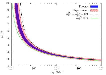
Figure 1: $\tan\beta$ as a function of $m_{0}$ for the observed Higgs mass. Red and blue bands show the experimental and theoretical uncertainties, respectively, for $\mu_{H}=m_{0}=m_{A^{0}}$ and all $\delta$’s and $\Delta$’s are set to be zero. The gaugino masses are set to be $M_{\tilde{B}}=600$ GeV, $M_{\tilde{W}}=300$ GeV, and $M_{\tilde{g}}=-2$ TeV. The cases of $\delta^{\tilde{Q}_{L}}_{13}=\delta^{\tilde{u}_{R}}_{13}=0.9$ (black line) and $\Delta^{\tilde{Q}_{L}}_{3}=4$ (green line) are also shown.

As we will see, the proton decay rate has strong dependence on $\tan\beta$. In Fig. 1, we show the predicted $\tan\beta$ for the observed Higgs mass as a function of the sfermion mass scale $m_{0}$. The red and blue bands show the experimental and theoretical uncertainties, respectively, for $\mu_{H}=m_{0}=m_{A^{0}}$ and all $\delta$’s and $\Delta$’s are zero. For the experimental inputs, see Table 1 in Appendix A. We estimate the theoretical error by changing the scale of matching between the MSSM and the (SM+gauginos) system from $m_{0}/3$ to $3m_{0}$. The gaugino masses are set to be $M_{\tilde{B}}=600$ GeV, $M_{\tilde{W}}=300$ GeV, and $M_{\tilde{g}}=-2$ TeV. We also show the cases of $\delta^{\tilde{Q}_{L}}_{13}=\delta^{\tilde{u}_{R}}_{13}=0.9$ (black line) and $\Delta^{\tilde{Q}_{L}}_{3}=4$ (green line). In this estimation, we use the two-loop renormalization group equations (RGEs) in the (SM + gauginos) system and the one-loop threshold effects from heavy sfermions and higgsinos. This figure illustrates that a relatively small value of $\tan\beta$ is favored in the high-scale SUSY scenario.

2.2 Flavor Constraints

The soft SUSY-breaking terms in general introduce new sources of flavor and CP violation, which are severely restricted by low-energy precision experiments [28]. As we will see, the flavor violation of squarks can strongly affect proton decay, and the slepton flavor violation not so much. In the rest of the section, we briefly review the current experimental constraints on the squark flavor mixing.

2.2.1 Meson Mixing

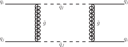
Figure 2: An example of the dominant diagram contributing to the meson mixings in the presence of the squark flavor mixing.

The $\Delta F=2$ meson mixings give strong constraints on the flavor violation $\delta$’s. The dominant contribution comes from the box diagram of Fig. 2. The contribution to the oscillation is represented by the following $\Delta F=2$ effective Hamiltonian,

$$H_{\rm eff}=\sum_{A=1}^{5}C_{A}O_{A}+\sum_{A=1}^{3}\tilde{C}_{A}\tilde{O}_{A},$$ (7)

where the operators $O_{A}$ and $\tilde{O}_{A}$ are defined as follows:

$$O_{1}=(\bar{q}^{\alpha}_{Li}\gamma_{\mu}q^{\alpha}_{Lj})(\bar{q}^{\beta}_{Li}\gamma^{\mu}q^{\beta}_{Lj}),$$

$$O_{2}=(\bar{q}^{\alpha}_{Ri}q^{\alpha}_{Lj})(\bar{q}^{\beta}_{Ri}q^{\beta}_{Lj}),~{}~{}~{}O_{3}=(\bar{q}^{\alpha}_{Ri}q^{\beta}_{Lj})(\bar{q}^{\beta}_{Ri}q^{\alpha}_{Lj}),$$

$$O_{4}=(\bar{q}^{\alpha}_{Ri}q^{\alpha}_{Lj})(\bar{q}^{\beta}_{Li}q^{\beta}_{Rj}),~{}~{}~{}O_{5}=(\bar{q}^{\alpha}_{Ri}q^{\beta}_{Lj})(\bar{q}^{\beta}_{Li}q^{\alpha}_{Rj}),$$ (8)

and $\tilde{O}_{A}$ by $R\leftrightarrow L$. In the large squark-mass limit, $m_{\tilde{q}}\gg m_{\tilde{g}}$, the dominant SUSY contributions to the Wilson coefficients are approximately given by

$$C_{1}\simeq\frac{11\alpha_{3}^{2}}{36}H(m^{2}_{\tilde{q}_{LI}},m^{2}_{\tilde{q}_{LJ}})(R^{\dagger}_{\tilde{q}_{L}})_{iI}(R_{\tilde{q}_{L}})_{Ij}(R^{\dagger}_{\tilde{q}_{L}})_{iJ}(R_{\tilde{q}_{L}})_{Jj},$$

$$C_{4}\simeq-\frac{\alpha_{3}^{2}}{3}H(m^{2}_{\tilde{q}_{RI}},m^{2}_{\tilde{q}_{LJ}})(R^{\dagger}_{\tilde{q}_{R}})_{iI}(R_{\tilde{q}_{R}})_{Ij}(R^{\dagger}_{\tilde{q}_{L}})_{iJ}(R_{\tilde{q}_{L}})_{Jj},~{}~{}C_{5}\simeq-\frac{5}{3}C_{4},$$

$$\tilde{C}_{1}\simeq\frac{11\alpha_{3}^{2}}{36}H(m^{2}_{\tilde{q}_{RI}},m^{2}_{\tilde{q}_{RJ}})(R^{\dagger}_{\tilde{q}_{R}})_{iI}(R_{\tilde{q}_{R}})_{Ij}(R^{\dagger}_{\tilde{q}_{R}})_{iJ}(R_{\tilde{q}_{R}})_{Jj},$$ (9)

where $H(x,y)=\log(x/y)/(x-y)$ and $R$’s are unitary matrices defined in Eq. (50). The other Wilson coefficients $C_{2},C_{3},\tilde{C}_{2}$ and $\tilde{C}_{3}$ are less significant in the present model.

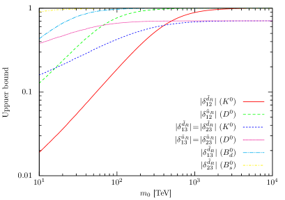
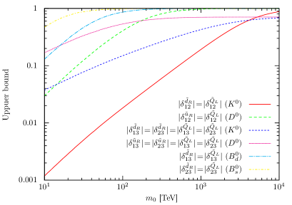
Figure 3: Upper-bound on the flavor violating mass terms $\delta$. (a): One chirality flavor violation (b): Both chirality flavor violation. We choose the “worst” case of the CP phases and take $M_{\tilde{B}}=600$ GeV, $M_{\tilde{W}}=300$ GeV, and $M_{\tilde{g}}=-2$ TeV.

In Fig. 3, we show the constraints on $\delta$’s from the meson mixings. The left (right) panel illustrates the case where flavor violation occurs in either (both) chirality. To get the constraints, we evolve the Wilson coefficients down to relevant hadronic scale and then use the results of new physics fits of Refs. [29, 30, 31]. The CP phase is chosen so that the strongest constraint is to be obtained. We set $M_{\tilde{B}}=600$ GeV, $M_{\tilde{W}}=300$ GeV, and $M_{\tilde{g}}=-2$ TeV in this plot. It is found that especially $\delta^{\widetilde{Q}_{L}}_{12}$ and $\delta^{\widetilde{d}_{R}}_{12}$ are stringently restricted from the $K^{0}$-$\bar{K}^{0}$ mixing even in the case of high-scale SUSY. Other flavor-violating parameters are allowed to be sizable when $m_{0}>10^{2}$ TeV. In the absence of CP violation, these constraints get less. Especially, constraints from $K^{0}$-$\bar{K}^{0}$ and $D^{0}$-$\bar{D}^{0}$ are greatly relaxed in the case of CP conservation, which allows $\delta$’s to be ${\cal O}(10)$ times larger.

2.2.2 EDM

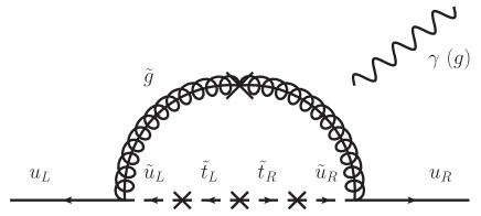
Figure 4: An example of the dominant diagram contributing to the EDMs and CEDMs of light quarks in the presence of the squark flavor mixing.

In the presence of CP violation, the electric dipole moments (EDMs) provide stringent limits on the flavor mixing in the sfermion masses, though the EDMs are flavor-conserving quantities in nature. As we shall see below, the dimension-five proton decay rate is quite sensitive to the squark flavor violation, which is constrained by the neutron EDM. On the assumption of the Peccei-Quinn mechanism [32] to solve the strong CP problem, the relevant effective operators of the lowest mass dimension are the EDMs and chromoelectric dipole moments (CEDMs) of light quarks. The CP violating effects induced by squarks are included into these two quantities. In Fig. 4, we show an example of the diagrams which yield the EDMs and the CEDMs. As illustrated in the diagram, the dominant contribution is given by the flavor-violating processes, where the mass terms of heavy quarks, especially that of top quark, flip the chirality. For instance, the EDM $d_{u}$ and CEDM $\tilde{d}_{u}$ of up quark are approximately give as

$$d_{u} \simeq-\frac{4}{3}\frac{\alpha_{3}}{4\pi}eQ_{u}\frac{m_{t}}{m_{0}^{4}}{\rm Im}\bigl{[}\mu_{H}M_{\widetilde{g}}\cot\beta\delta^{\widetilde{Q}_{L}}_{13}\delta^{\widetilde{u}_{R}*}_{13}\bigr{]}~{},$$

$$\tilde{d}_{u} \simeq 6\frac{\alpha_{3}}{4\pi}\frac{m_{t}}{m_{0}^{4}}\ln\biggl{(}\frac{m_{0}}{|M_{\widetilde{g}}|}\biggr{)}{\rm Im}\bigl{[}\mu_{H}M_{\widetilde{g}}\cot\beta\delta^{\widetilde{Q}_{L}}_{13}\delta^{\widetilde{u}_{R}*}_{13}\bigr{]}~{},$$ (10)

with $eQ_{u}$ the charge of up quark. Similar expressions hold for down and strange quarks. Notice that both the left-handed and right-handed squark mixings are required to utilize the enhancement by heavy quark masses. By evaluating the contribution with the renormalization group improved method described in Ref. [35], we obtain constraints on the flavor mixing parameters from the current experimental bound on the neutron EDM, $|d_{n}|<2.9\times 10^{-26}~{}e\cdot{\rm cm}$ [36]. The results are shown in Fig. 5. In the figure, the purple, blue, red, and green lines show the constraints on $|\delta_{13}^{\widetilde{Q}_{L}}|=|\delta_{13}^{\widetilde{u}_{R}}|$, $|\delta_{13}^{\widetilde{Q}_{L}}|=|\delta_{13}^{\widetilde{d}_{R}}|$, $|\delta_{12}^{\widetilde{Q}_{L}}|=|\delta_{12}^{\widetilde{u}_{R}}|$, and $|\delta_{12}^{\widetilde{Q}_{L}}|=|\delta_{12}^{\widetilde{d}_{R}}|$, respectively, as functions of the sfermion mass scale $m_{0}$. We take $M_{\tilde{B}}=600$ GeV, $M_{\tilde{W}}=300$ GeV, $M_{\tilde{g}}=-2$ TeV, and $\mu_{H}=m_{0}$. In the calculation, we use

$$d_{n}=0.79d_{d}-0.20d_{u}+e(0.30\tilde{d}_{u}+0.59\tilde{d}_{d})~{}$$ (11)

to estimate the neutron EDM, which is obtained by using the method of the QCD sum rules [37]. The figure illustrates that ${\cal O}(1)$ flavor mixing results in constraints on the sfermion mass scale as high as ${\cal O}(10^{2})$ TeV.

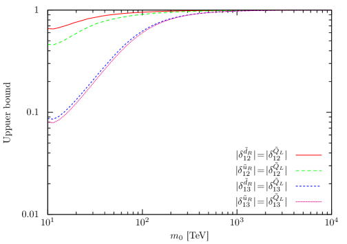
Figure 5: Constraints on flavor mixing parameters as functions of sfermion mass scale $m_{0}$. Purple, blue, red, and green lines illustrate constraints on $|\delta_{13}^{\widetilde{Q}_{L}}|=|\delta_{13}^{\widetilde{u}_{R}}|$, $|\delta_{13}^{\widetilde{Q}_{L}}|=|\delta_{13}^{\widetilde{d}_{R}}|$, $|\delta_{12}^{\widetilde{Q}_{L}}|=|\delta_{12}^{\widetilde{u}_{R}}|$, and $|\delta_{12}^{\widetilde{Q}_{L}}|=|\delta_{12}^{\widetilde{d}_{R}}|$, respectively. We take $M_{\tilde{B}}=600$ GeV, $M_{\tilde{W}}=300$ GeV, $M_{\tilde{g}}=-2$ TeV, $\tan\beta=5$ and $\mu_{H}=m_{0}$.

3 Proton Decay with Sfermion Flavor Violation

3.1 Minimal SUSY SU(5) GUT

In this section, we give a short review on the minimal SUSY SU(5) GUT [39, 40] to clarify our notation and conventions used in this paper. Just like the Georgi-Glashow SU(5) model [41], the MSSM matter fields are embedded in a $\bar{\bf 5}\oplus{\bf 10}$ representation; the SU(2)_L singlet down-type quarks $\bar{d}_{i}$ and doublet leptons $L_{i}$ are in the $\bar{\bf 5}$ fields, $\Phi_{i}$, while the SU(2)_L singlet up-type quarks, $\bar{u}_{i}$, doublet quarks, $Q_{i}$, and singlet leptons, $\bar{e}_{i}$, are in the ${\bf 10}$ representations, $\Psi_{i}$. The MSSM Higgs superfields, $H_{u}$ and $H_{d}$, are incorporated into a pair of 5 and $\bar{\bf 5}$ superfields and their SU(5) partners $H_{C}$ and $\bar{H}_{C}$ are called the color-triplet Higgs multiplets. The gauge vector multiplets are embedded into an adjoint vector multiplet. The new gauge fields introduced to form the adjoint representation are called the $X$-bosons, and they acquire masses of the order of the GUT scale after the SU(5) gauge group is broken into the SM gauge group by the VEV of an adjoint Higgs boson.

In the minimal SUSY SU(5) GUT, the Yukawa interactions originate from the following superpotential:

$$W_{\rm Yukawa} =\frac{1}{4}h^{ij}\epsilon_{\hat{a}\hat{b}\hat{c}\hat{d}\hat{e}}\Psi_{i}^{\hat{a}\hat{b}}\Psi_{j}^{\hat{c}\hat{d}}H^{\hat{e}}-\sqrt{2}f^{ij}\Psi_{i}^{\hat{a}\hat{b}}\Phi_{j\hat{a}}\bar{H}_{\hat{b}}~{},$$ (12)

where $\hat{a},\hat{b},\dots=1$–$5$ represent the SU(5) indices; $\epsilon_{\hat{a}\hat{b}\hat{c}\hat{d}\hat{e}}$ is the totally antisymmetric tensor with $\epsilon_{12345}=1$; $h^{ij}$ is symmetric with respect to the generation indices $i,j$. The field re-definition of $\Psi$ and $\Phi$ reveals that the number of the physical degrees of freedom in $h^{ij}$ and $f^{ij}$ is twelve. Among them, six is for quark mass eigenvalues and four is for the CKM matrix elements, so we have two additional phases [42].

These Yukawa terms are matched to the MSSM Yukawa couplings at the GUT scale. Note that the generation basis of the MSSM superfields may be different from that of the SU(5) superfields $\Psi_{i}$ and $\Phi_{i}$. To take the difference into account, we write the relation between the SU(5) components and the MSSM superfields as

$$\Psi_{i} \ni\{Q_{i},~{}(V_{QU})_{ij}\overline{u}_{j},~{}(V_{QE})_{ij}\overline{e}_{j}\}~{},$$

$$\Phi_{i} \ni\{\overline{d}_{i},~{}(V_{DL})_{ij}L_{j}\}~{},$$ (13)

where $V_{QU}$, $V_{QE}$, and $V_{DL}$ are unitary matrices, which play a similar role to the CKM matrix. In this paper, we take them as

$$V_{QU}=P^{*}~{},~{}~{}~{}~{}~{}~{}V_{QE}=V_{\rm CKM}(M_{\rm GUT})~{},~{}~{}~{}~{}~{}~{}V_{DL}=\mbox{1}\mbox{l}~{},$$ (14)

where $P$ is a diagonal phase matrix with $\det P=1$ and $V_{\rm CKM}(M_{\rm GUT})$ is the CKM matrix at the GUT scale. Then, we have the matching condition as follows:

$$h^{ij}=(P\hat{f}_{u}(M_{\rm GUT}))^{ij}~{},$$

$$f^{ij}=(V^{*}\hat{f}_{d}(M_{\rm GUT}))^{ij}~{},$$

$$\hat{f}_{d}(M_{\rm GUT})=\hat{f}_{e}(M_{\rm GUT})~{},$$ (15)

where $\hat{f}_{u}$, $\hat{f}_{d}$, and $\hat{f}_{e}$ are diagonal and non-negative Yukawa matrices of the up-type quarks, the down-type quarks, and the charged leptons, respectively, and $V\equiv V_{\rm CKM}(M_{\rm GUT})$. In this basis, the Yukawa terms are written in terms of the MSSM superfields as

$$W_{\rm Yukawa} =(\hat{f}_{u})^{ij}(Q^{a}_{i}\cdot H_{u})\overline{u}_{ja}-(V^{*}\hat{f}_{d})^{ij}(Q^{a}_{i}\cdot H_{d})\overline{d}_{ja}-(\hat{f}_{e})^{ij}\overline{e}_{i}(L_{j}\cdot H_{d})$$

$$-\frac{1}{2}(P\hat{f}_{u})^{ij}\epsilon_{abc}(Q^{a}_{i}\cdot Q^{b}_{j})H^{c}_{C}+(V^{*}\hat{f}_{d})^{ij}(Q^{a}_{i}\cdot L_{j})\overline{H}_{Ca}$$

$$+(\hat{f}_{u}V)^{ij}\overline{u}_{ia}\overline{e}_{j}H^{a}_{C}-(P^{*}V^{*}\hat{f}_{d})^{ij}\epsilon^{abc}\overline{u}_{ia}\overline{d}_{jb}\overline{H}_{Cc}~{}.$$ (16)

Here, $(A\cdot B)\equiv\epsilon^{\alpha\beta}A_{\alpha}B_{\beta}$ with $\alpha,\beta$ representing the SU(2)_L indices, and $a,b,c$ denote the color indices. As it can be seen from the above expression, we have chosen our basis so that the Yukawa couplings of the up-type quarks and the charged leptons are diagonalized.

3.2 Dimension-Five Proton Decay

Now we discuss the proton decay via the color-triplet Higgs exchange . We first give a set of formulae used in the following calculation of the proton decay rate.

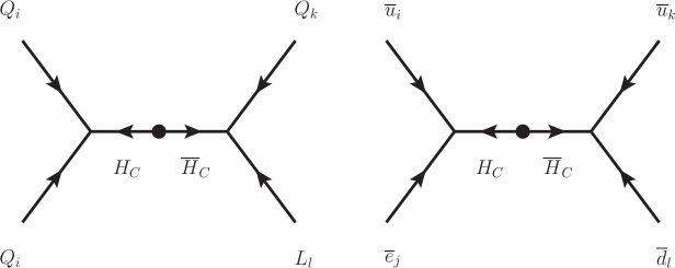
Figure 6: Supergraphs for color-triplet Higgs exchanging processes where dimension-five effective operators for proton decay are induced. Bullets indicate color-triplet Higgs mass term.

The Yukawa interactions of color-triplet Higgs multiplets, which are displayed in Eq. (16), give rise to the dimension-five proton decay operators [43, 44]. The diagrams which induce the operators are illustrated in Fig. 6. By integrating out the color-triplet Higgs multiplets, we obtain the effective Lagrangian

$${\cal L}_{5}^{\rm eff}=C^{ijkl}_{5L}{\cal O}^{5L}_{ijkl}+C^{ijkl}_{5R}{\cal O}^{5R}_{ijkl}~{}~{}+~{}~{}{\rm h.c.}~{},$$ (17)

where the effective operators ${\cal O}^{5L}_{ijkl}$ and ${\cal O}^{5R}_{ijkl}$ are defined by

$${\cal O}^{5L}_{ijkl} \equiv\int d^{2}\theta~{}\frac{1}{2}\epsilon_{abc}(Q^{a}_{i}\cdot Q^{b}_{j})(Q_{k}^{c}\cdot L_{l})~{},$$

$${\cal O}^{5R}_{ijkl} \equiv\int d^{2}\theta~{}\epsilon^{abc}\overline{u}_{ia}\overline{e}_{j}\overline{u}_{kb}\overline{d}_{lc}~{},$$ (18)

and the Wilson coefficients $C^{ijkl}_{5L}$ and $C^{ijkl}_{5R}$ are given by

$$C^{ijkl}_{5L}(M_{\rm GUT}) =+\frac{1}{M_{H_{C}}}(P\hat{f}_{u})^{ij}(V^{*}\hat{f}_{d})^{kl}~{},$$

$$C^{ijkl}_{5R}(M_{\rm GUT}) =+\frac{1}{M_{H_{C}}}(\hat{f}_{u}V)^{ij}(P^{*}V^{*}\hat{f}_{d})^{kl}~{}.$$ (19)

Here, $M_{H_{C}}$ is the mass of color-triplet Higgs multiplets. Note that because of the totally antisymmetric tensor in the operators ${\cal O}^{5L}_{ijkl}$ and ${\cal O}^{5R}_{ijkl}$ they must include at least two generations of quarks. For this reason, the dominant mode of proton decay induced by the operators is accompanied by strange quarks; like the $p\to K^{+}\bar{\nu}$ mode. The Wilson coefficients in Eq. (19) are determined at the GUT scale. To evaluate the proton decay rate, we need to evolve them down to low-energy regions by using the RGEs. The RGEs for the coefficients are presented in Appendix B.

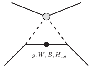
Figure 7: One-loop diagram which yields proton decay four-Fermi operators. The gray dot indicates the dimension-five effective interactions and black dot represents the mass term of exchanged particles; gauginos or higgsinos.

The dimension-five operators contain sfermions in their external lines. At the sfermion mass scale $m_{0}$, sfermions decouple from the theory, and the dimension-five operators reduce to the dimension-six four-Fermi operators via the exchange of gauginos and higgsinos. In Fig. 7, an one-loop diagram which yields the four-Fermi operators is illustrated. Here, the gray dot indicates the dimension-five effective interactions and the black dot represents the mass term of exchanged particles. The four-Fermi operators induced here are written in an invariant form under the SU(3)${}_{C}\otimes$SU(2)${}_{L}\otimes$U(1)_Y symmetry. A set of such operators is summarized in Refs [45, 46, 47] as follows:

$${\cal O}^{(1)}_{ijkl} =\epsilon_{abc}(u^{a}_{Ri}d^{b}_{Rj})(Q_{Lk}^{c}\cdot L_{Ll})~{},$$

$${\cal O}^{(2)}_{ijkl} =\epsilon_{abc}(Q^{a}_{Li}\cdot Q^{b}_{Lj})(u_{Rk}^{c}e_{Rl})~{},$$

$${\cal O}^{(3)}_{ijkl} =\epsilon_{abc}\epsilon^{\alpha\beta}\epsilon^{\gamma\delta}(Q^{a}_{Li\alpha}Q^{b}_{Lj\gamma})(Q_{Lk\delta}^{c}L_{Ll\beta})~{},$$

$${\cal O}^{(4)}_{ijkl} =\epsilon_{abc}(u^{a}_{Ri}d^{b}_{Rj})(u_{Rk}^{c}e_{Rl})~{}.$$ (20)

Here we explicitly write the way of contracting the SU(2)_L indices for ${\cal O}^{(3)}_{ijkl}$. Let us express their Wilson coefficients by $C^{ijkl}_{(I)}$ for ${\cal O}^{(I)}_{ijkl}$ $(I=1,2,3,4)$. Then, they are matched with $C_{5L}^{ijkl}$ and $C_{5R}^{ijkl}$ at the SUSY breaking scale. The matching conditions are summarized in Appendix C.1. Again, the coefficients are evolved down to the electroweak scale according to the RGEs. The RGEs below the SUSY breaking scale are also given in Appendix B.

Below the electroweak scale $\mu=m_{Z}$, the effective operators are no longer invariant under the SU(3)${}_{C}\otimes$SU(2)${}_{L}\otimes$U(1)_Y symmetry; instead, they must respect the SU(3)${}_{C}\otimes$U(1)_em, and all of the fields in the operators are to be written in the mass basis. As mentioned above, the dominant mode of proton decay induced by the dimension-five effective operators is the $p\to K^{+}\bar{\nu}$ mode. The effective Lagrangian which yields the decay mode is written down as follows:

$${\cal L}(p\to K^{+}\bar{\nu}_{i})= C_{RL}(dsu\nu_{i})\bigl{[}\epsilon_{abc}(d_{R}^{a}s_{R}^{b})(u_{L}^{c}\nu_{i})\bigr{]}+C_{RL}(usd\nu_{i})\bigl{[}\epsilon_{abc}(u_{R}^{a}s_{R}^{b})(d_{L}^{c}\nu_{i})\bigr{]}$$

$$+ C_{RL}(uds\nu_{i})\bigl{[}\epsilon_{abc}(u_{R}^{a}d_{R}^{b})(s_{L}^{c}\nu_{i})\bigr{]}+C_{LL}(dsu\nu_{i})\bigl{[}\epsilon_{abc}(d_{L}^{a}s_{L}^{b})(u_{L}^{c}\nu_{i})\bigr{]}$$

$$+ C_{LL}(usd\nu_{i})\bigl{[}\epsilon_{abc}(u_{L}^{a}s_{L}^{b})(d_{L}^{c}\nu_{i})\bigr{]}+C_{LL}(uds\nu_{i})\bigl{[}\epsilon_{abc}(u_{L}^{a}d_{L}^{b})(s_{L}^{c}\nu_{i})\bigr{]}~{}.$$ (21)

Here, all of the fermions are written in terms of the mass eigenstates. The matching condition for the Wilson coefficients $C_{RL}$ and $C_{LL}$ at the electroweak scale are listed in Appendix C.2.

The Wilson coefficients are taken down to the hadronic scale $\mu=2$ GeV, where the matrix elements of the effective operators are evaluated. The RGEs for the step are given in Appendix B. For the hadron matrix elements of the effective operators, we use the results presented by the lattice QCD calculation [48]. Their values are listed in Table 2 in Appendix A. By using the results, we can eventually obtain the partial decay width of the $p\to K^{+}\bar{\nu}_{i}$ mode as

$$\Gamma(p\to K^{+}\bar{\nu}_{i})=\frac{m_{p}}{32\pi}\biggl{(}1-\frac{m_{K}^{2}}{m_{p}^{2}}\biggr{)}^{2}|{\cal A}(p\to K^{+}\bar{\nu}_{i})|^{2}~{},$$ (22)

where $m_{p}$ and $m_{K}$ are the masses of proton and kaon, respectively. The amplitude ${\cal A}(p\to K^{+}\bar{\nu}_{i})$ is given by the sum of the Wilson coefficients at $\mu=2$ GeV multiplied by the corresponding hadron matrix elements.

By following a similar procedure, we can also evaluate the partial decay rates for other modes. The resultant expressions are presented in Appendix D.

3.3 Results

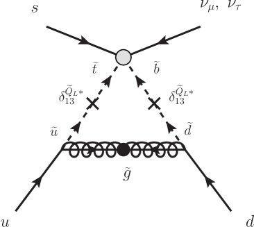
Figure 8: Diagram which induces the dominant contribution in the presence of the $\delta^{\widetilde{Q}_{L}}_{13}$ flavor mixing, which is denoted by $\times$-mark.

As discussed in Ref. [49], the charged wino and higgsino exchange processes give rise to the dominant contribution to the dimension-five proton decay in the case of the minimal flavor violation. When the sfermion sector contains sizable flavor violation, on the other hand, not only the charged fermions, but also the neutral gauginos and higgsinos can contribute. Especially, the gluino contribution becomes significant because of the large value of $\alpha_{3}$. Since only the $C^{ijkl}_{(3)}|_{\widetilde{g}}$ in Eq. (48) contributes to the $p\to K^{+}\bar{\nu}$ proton decay, the flavor mixing in the mass matrix of $\widetilde{Q}_{L}$ is most important; in particular $\delta^{\widetilde{Q}_{L}}_{13}$ gives rise to the biggest effects. Let us estimate the significance. The dominant contribution to the $p\to K^{+}\bar{\nu}$ mode is induced by the diagram in Fig. 8. Here, the cross-mark indicates the flavor mixing. When the flavor violation is small but sizable, e.g., $\delta^{\widetilde{Q}_{L}}_{13}\sim 0.1$, the contribution is evaluated as

$$C_{LL}(uds\nu_{\mu}) \simeq-\frac{4}{3}\frac{\alpha_{2}\alpha_{3}}{\sin 2\beta}\frac{m_{t}m_{s}}{M_{H_{C}}m_{W}^{2}}\frac{M_{\widetilde{g}}}{m_{0}^{2}}~{}e^{i\varphi_{3}}(V_{ud}V_{cs}V_{cs}^{*})\bigl{(}\delta^{\widetilde{Q}_{L}*}_{13}\bigr{)}^{2}~{},$$

$$C_{LL}(uds\nu_{\tau}) \simeq-\frac{4}{3}\frac{\alpha_{2}\alpha_{3}}{\sin 2\beta}\frac{m_{t}m_{b}}{M_{H_{C}}m_{W}^{2}}\frac{M_{\widetilde{g}}}{m_{0}^{2}}~{}e^{i\varphi_{3}}(V_{ud}V_{cs}V_{cb}^{*})\bigl{(}\delta^{\widetilde{Q}_{L}*}_{13}\bigr{)}^{2}~{},$$ (23)

and other Wilson coefficients are found to be sub-dominant. Here, we assume $M_{\widetilde{g}}\ll m_{0}$. As we have mentioned above, the contribution strongly depends on $\tan\beta$. By comparing the results to the higgsino contribution in the minimal flavor violation case, which is found to be dominant when $\mu_{H}\simeq m_{0}$ [16], we can see that the gluino contribution becomes dominant when

$$\bigl{|}\delta^{\widetilde{Q}_{L}}_{13}\bigr{|}~{}\gtrsim~{}2\times 10^{-3}\times\biggl{(}\frac{1}{\sin 2\beta}\biggl{|}\frac{\mu_{H}}{M_{\widetilde{g}}}\biggr{|}\biggr{)}^{\frac{1}{2}}~{}.$$ (24)

Before showing the results for the full computation, we briefly comment on the features of other contributions. The wino and bino contributions are in general suppressed by the relatively small gauge couplings compared with the gluino contribution. The higgsino contribution has already exploited the flavor changing in the Yukawa couplings to make the most of the enhancement from the third generation Yukawa couplings. Therefore, the flavor mixing in sfermion masses does not increase the contribution any more.

As we will see below, the effects of the other mixing parameters are generally sub-dominant. In particular, when the flavor violation occurs only in the slepton sector, the proton decay rate is rarely changed. This is because the gluino exchange process does not contribute to the proton decay in such a case. In addition, when only the right-handed squarks feel the flavor violation, the $p\to K^{+}\bar{\nu}$ mode is not enhanced because of the same reason. In such a case, on the other hand, the decay modes including a charged lepton in their final states, such as the $p\to\pi^{0}\mu^{+}$ mode, are considerably enhanced. We will discuss the feature in more detail below.

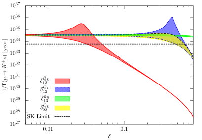
(a) $p\to K^{+}\bar{\nu}$

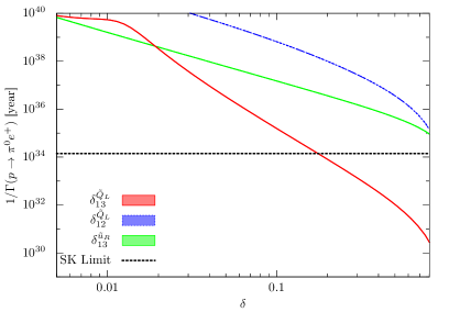
(b) $p\to\pi^{0}e^{+}$

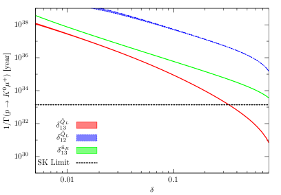
(c) $p\to K^{0}\mu^{+}$

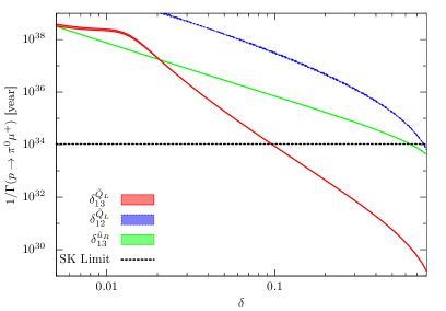
(d) $p\to\pi^{0}\mu^{+}$

Figure 9: Proton lifetime as functions of flavor mixing parameters $\delta$’s. Red, blue, green, and yellow lines correspond to $\delta^{\widetilde{Q}_{L}}_{13}$, $\delta^{\widetilde{Q}_{L}}_{12}$, $\delta^{\widetilde{u}_{R}}_{13}$, and $\delta^{\widetilde{Q}_{L}}_{23}$, respectively. The color bands show the uncertainty from unknown CP phases $P$ in the GUT Yukawa couplings defined in Eq. (14). We set $m_{0}=100$ TeV, $M_{\tilde{B}}=600$ GeV, $M_{\tilde{W}}=300$ GeV, $M_{\tilde{g}}=-2$ TeV, $\tan\beta=5$, $\mu_{H}=+m_{0}$, and $M_{H_{C}}=10^{16}$ GeV. $\Delta$’s and $\delta$’s which are not displayed in the figure are set to be zero. Black dashed lines represent the experimental limits presented by Super-Kamiokande [50, 51].

Now we show the results. In Fig. 9, we show the proton lifetime as functions of selected flavor violating parameters $\delta$’s in Eq. (5). The red, blue, green, and yellow lines correspond to $\delta^{\widetilde{Q}_{L}}_{13}$, $\delta^{\widetilde{Q}_{L}}_{12}$, $\delta^{\widetilde{u}_{R}}_{13}$, and $\delta^{\widetilde{Q}_{L}}_{23}$, respectively. In this figure, the uncertainty coming from the unknown phases $P$ in the GUT Yukawa couplings defined in Eq. (14) is shown as color bands. We take $m_{0}=100$ TeV, $M_{\tilde{B}}=600$ GeV, $M_{\tilde{W}}=300$ GeV , $M_{\tilde{g}}=-2$ TeV, and $\tan\beta=5$, $\mu_{H}=+m_{0}$, and $M_{H_{C}}=10^{16}$ GeV, and we do not include the running effects on the gaugino masses. The black dashed lines represent the experimental limits presented by Super-Kamiokande [50, 51]. From the figure, it is found that $\delta^{\tilde{Q}_{L}}_{13}$ gives strong impacts on the proton lifetime for each decay channel. It results from the large contribution of gluino exchange processes to the proton decay rates. For instance, in the case of the $p\to K^{+}\bar{\nu}$ decay mode given in the plot (a), gluino dressing parts become dominant when $\delta^{\tilde{Q}_{L}}_{13}\gg 0.01$. In the region, the proton partial decay rate is approximately proportional to the fourth power of $\delta^{\tilde{Q}_{L}}_{13}$, as described in Eq. (23). For small $\delta^{\tilde{Q}_{L}}_{13}\ll 0.01$, on the other hand, the higgsino dressing contribution dominates the decay amplitude, and thus the lifetime hardly depends on the flavor violation. When $\delta^{\tilde{Q}_{L}}_{13}\sim 0.01$, both gluino and higgsino dressing contributions are comparable to each other, which may result in a significant cancellation between them, depending on the GUT CP phases $P$.

We also present the results for the $p\to\pi^{0}e^{+}$, $p\to K^{0}\mu^{+}$, and $p\to\pi^{0}\mu^{+}$ channel in the plots (b), (c), and (d) in Fig. 9, respectively. A characteristic feature in this case is that the right-handed squark flavor violation, such as $\delta^{\widetilde{u}_{R}}_{13}$ and $\delta^{\widetilde{d}_{R}}_{13}$, is also important. This is because when the final state of proton decay includes a charged lepton, not only the operators ${\cal O}^{(1)}_{ijkl}$ and ${\cal O}^{(3)}_{ijkl}$ but also ${\cal O}^{(2)}_{ijkl}$ and ${\cal O}^{(4)}_{ijkl}$ can contribute to the decay rate. Notice that in the gluino exchange process the right-handed squark flavor violation can only contribute to the operator ${\cal O}^{(4)}_{ijkl}$, as can been seen from the formulae presented in Appendix D. For this reason, $\delta^{\widetilde{u}_{R}}_{13}$ and $\delta^{\widetilde{d}_{R}}_{13}$ scarcely affect the anti-neutrino decay modes such as $p\to K^{+}\bar{\nu}$, which are induced by the operator ${\cal O}^{(3)}_{ijkl}$, while they can enhance the charged lepton modes through ${\cal O}^{(4)}_{ijkl}$.

The sfermion flavor violation also alters the branching ratio. This can be again seen from the plots (b–d) in Fig. 9; without flavor violation, the decay rates of these modes are extremely small compared with that of $p\to K^{+}\bar{\nu}$, while they become significant in the presence of sizable flavor violation. To see the feature more clearly, we show the partial decay rates of selected proton decay modes for various $\delta$’s in Fig. 10. The red bars show the case in which we take $m_{0}=100$ TeV, $M_{\tilde{B}}=600$ GeV, $M_{\tilde{W}}=300$ GeV, $M_{\tilde{g}}=-2$ TeV, $\tan\beta=5$, $\mu_{H}=+m_{0}$, and $M_{H_{C}}=10^{16}$ GeV, while the green bars correspond to the case where the gaugino masses are ten times as large as the previous ones: $M_{\tilde{B}}=6$ TeV, $M_{\tilde{W}}=3$ TeV, and $M_{\tilde{g}}=-20$ TeV. The bar charts in Fig. 10 illustrate the features of the dimension-five proton decay discussed above; in the case of the minimal flavor violation, the most significant decay mode is the $p\to K^{+}\bar{\nu}$ channel, while other decay modes get also viable once you switch on the flavor violation; $\delta^{\widetilde{Q}_{L}}_{13}$ yields the most significant effects on the proton decay rate, contrary to the flavor violation in slepton mass matrices, which gives little contribution; $\delta^{\tilde{u}_{R}}_{13}$ enhances the decay rates of the charged lepton modes, rather than those of the anti-neutrino modes such as $p\to K^{+}\bar{\nu}$.

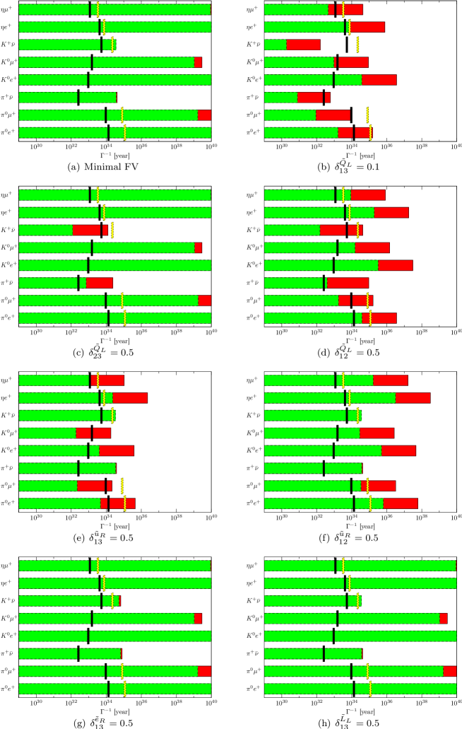
Figure 10: Dependence of the proton decay modes on the flavor structure. Red bars show the case where a similar set of parameters to those in Fig. 9 is taken, while green bars correspond to the case in which the gaugino masses are ten times as large as the previous ones. Black lines represent the Super-Kamiokande constraints at 90 % CL while yellow lines show the future prospects of Hyper-Kamiokande [50, 51].

Now let us look for a specific signature of the proton decay associated with sfermion flavor violation. As one can see from Fig. 10, in the minimal flavor violation case, only the anti-neutrino decay modes, $p\to K^{+}\bar{\nu}$ and $p\to\pi^{+}\bar{\nu}$, have sizable decay rates. To distinguish the flavor violating contribution from it, therefore, we should focus on the charged lepton decay modes. As shown in Sec. 3.6.3, charged leptonic decay is also induced via the $X$-boson exchanging process. Since the process is induced by the gauge interactions, the CKM matrix is the only source for the flavor violation. Thus, in the $X$-boson exchange contribution, the decay modes which include different generations in their final states, such as $p\to\pi^{0}\mu^{+}$ and $p\to K^{0}e^{+}$, suffer from the CKM suppression. We will see this feature in Sec. 3.6.3. Hence, such decay modes can be regarded as characteristic of extra flavor violation if they are actually observed. Among them, the experimental constraint on the $p\to\pi^{0}\mu^{+}$ mode is the severest, and thus it may offer a good prove for the sfermion flavor violation. If the decay process as well as the $p\to K^{+}\bar{\nu}$ decay is detected in future experiments, it may suggest the existence of sizable flavor violation in the sfermion sector.

After all, in the presence of sfermion flavor violation, which can naturally be sizable in the high-scale SUSY scenario, a variety of proton decay modes may lie in a region which can be probed in future proton decay experiments. In consequence, proton decay experiments might shed light on SUSY even though it is broken at a relatively high-scale, and provide a way of investigating the structure of sfermion sector.

3.4 Flavor Constraints from Proton Decay

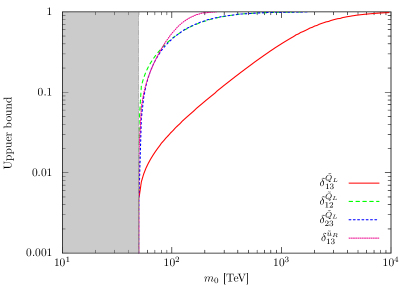
(a) Light gauginos

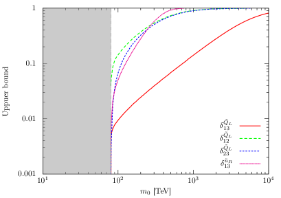
(b) Heavy gauginos

Figure 11: Upper-bound on the flavor violating mass terms $\delta$ from proton decay. Red, green, blue, and purple lines correspond to $\delta^{\widetilde{Q}_{L}}_{13}$, $\delta^{\widetilde{Q}_{L}}_{12}$, $\delta^{\widetilde{Q}_{L}}_{23}$, and $\delta^{\widetilde{u}_{R}}_{13}$, respectively. We take $M_{H_{C}}=10^{16}$ GeV, $\mu_{H}=m_{0}$ and $\tan\beta=5$. (a): $M_{\tilde{B}}=600$ GeV, $M_{\tilde{W}}=300$ GeV, and $M_{\tilde{g}}=-2$ TeV. (b): $M_{\tilde{B}}=6$ TeV, $M_{\tilde{W}}=3$ TeV, and $M_{\tilde{g}}=-20$ TeV. The shaded gray regions show the case that the proton decay rate conflicts the current experimental limits, even when all $\delta$’s and $\Delta$’s are zero. GUT phases $P$ (defined in Eq. (14)) are taken so that the strongest bounds on $\delta$’s are obtained.

As we have seen above, the sfermion flavor violations accelerate the proton decay rate from the dimension-five operators. Therefore, in the context of the minimal SU(5) GUT, the absence of observation of proton decay gives constraints on the sfermion flavor violations. In Fig. 11, we show the upper-bound on the size of flavor-violation $\delta$’s. Compared to the constrains from the meson mixings (Fig. 3) and the EDM (Fig. 5), the proton decay stringently constrains $\delta^{\tilde{Q}_{L}}_{13}$. As a result, less (up-)quark EDM is predicted in the minimal SU(5) GUT. In other words, future discovery of the quark EDM’s can exclude large parameter space of the minimal SU(5) GUT model.

3.5 Uncertainty of Decay Rate

Here we briefly discuss uncertainties of estimation of the proton decay rate. The most significant uncertainty comes from error of the hadron matrix elements in Table 2. This provides a factor 10 uncertainty for the proton decay rate. The effects of the experimental parameter inputs shown in Table 1 are relatively minor. Another important uncertainty comes from the short-distance parameters. In addition to the color-triplet higgsino mass $M_{H_{C}}$, the proton decay is quite sensitive to the Yukawa and gauge couplings at the high-energy regions. In our analysis, however, we do not include finite threshold effects from the sfermions and GUT sector, and thus our result cannot achieve accuracy beyond the one-loop RGE. To estimate possible contributions from higher order corrections we ignore, we also study (incomplete) two-loop level RGEs.

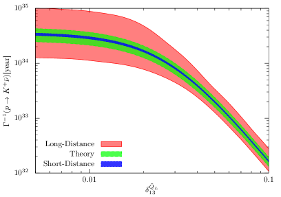
Figure 12: Error estimation of the proton decay rate. We show (one-sigma) error bands. The SUSY mass spectrum is same as that in Fig. 9. Red region displays the uncertainty from the error of the matrix elements shown in Table 2. Blue represents uncertainty from the error of the input parameters shown in Table 1. Green is the theoretical uncertainties.

In Fig. 12, we show the uncertainties in the case of $p\to K^{+}\bar{\nu}$ mode. The SUSY mass spectrum is same as that in Fig. 9. The red region displays the uncertainty from the error of the matrix elements, while blue represents that from the input parameters in Table 1. The green band shows the theoretical uncertainty, which we regard as the difference between results with the one- and two-loop RGEs. We will discuss other contributions which may alter our present analysis in the subsequent subsection.

3.6 Possible Additional Corrections

Here, we consider additional corrections which may be sizable in some particular cases.

3.6.1 Threshold Correction to Yukawa Couplings

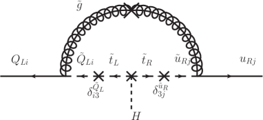
Figure 13: An example of threshold corrections to Yukawa couplings.

In the present analysis, we ignore the threshold corrections to the Yukawa couplings from sfermions as well as the GUT-scale particles or some Planck suppressed operators. However, depending on the parameter, these corrections may get significant. Let us first discuss the threshold corrections at the sfermion mass scale. In Fig. 13, we show an example of such corrections. In this case, the size of the correction is roughly given by

$$\delta f^{\rm MSSM}_{ij}\sim\frac{9}{8}\frac{f_{t}\alpha_{3}\mu_{H}^{*}M^{*}_{\tilde{g}}}{4\pi m_{0}^{2}\tan\beta}\delta^{\tilde{Q}_{L}}_{i3}\delta^{\tilde{u}_{R}*}_{j3}.$$ (25)

Therefore, large flavor violation in the sfermion sector possibly leads to significant corrections to the Yukawa couplings. However note that similar processes may also give rise to EDMs in the presence of CP violation, as discussed in Sec. 2.2.2. Therefore, we expect these threshold effects to be small as long as we consider the parameter region which evades the current limits from the EDM experiments.

The minimal SUSY SU(5) GUT predicts the unification of down-type quark and lepton Yukawa couplings as in Eq. (15). However, in the present parameter space, it is difficult to achieve the successful Yukawa unification. This means that we omit some corrections to the Yukawa couplings, such as those from the GUT-scale particles or some higher-dimensional operators induced at the Planck scale. With our ignorance of such corrections, we expect there is an ${\cal O}((f_{d}-f_{e})_{\rm GUT})$ uncertainty of estimation of the Yukawa couplings at the GUT scale. It may significantly affect the prediction of the proton decay rate. A detailed analysis will be done elsewhere [52].

3.6.2 Contribution from Soft Baryon-number Violating Operator

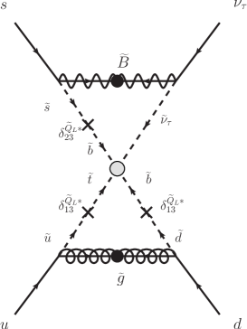
Figure 14: Contribution of the soft terms for the dimension-five operators to proton decay, which turns out to vanish.

Up to now, we only consider the dimension-five effective operators which are exactly supersymmetric. However, through the supergravity effects, the $A$-terms corresponding to these operators are also induced [53, 54]. This can be readily understood by means of the superconformal compensator formalism of supergravity [55]. In this formalism, the dimension-five operators should be accompanied by the compensator $\Sigma$ as

$$\int d^{2}\theta~{}\frac{1}{\Sigma}\biggl{[}C^{ijkl}_{5L}{\cal O}_{ijkl}^{5L}+C^{ijkl}_{5R}{\cal O}_{ijkl}^{5R}\biggr{]}~{}.$$ (26)

Then, after the compensator gets the $F$-term VEV as $\langle\Sigma\rangle=1+m_{3/2}\theta^{2}$, the dimension-four soft-terms are induced. The leading terms are given as

$${\cal L}_{\rm soft}=-\frac{C^{L}_{ijkl}m_{3/2}}{2M_{Hc}}\widetilde{Q}_{Li}\widetilde{Q}_{Lj}\widetilde{Q}_{Lk}\widetilde{L}_{Ll}-\frac{C^{R}_{ijkl}m_{3/2}}{M_{Hc}}\widetilde{u}_{Ri}^{*}\widetilde{d}_{Rj}^{*}\widetilde{u}_{Rk}^{*}\widetilde{e}_{Rl}^{*}~{}~{}+{\rm h.c.}~{}.$$ (27)

These soft terms also generate the proton decay four-Fermi operators via two-loop diagrams with the exchange of gauginos and higgsinos. This contribution is suppressed by additional factor $g^{2}/(16\pi^{2})(M_{\tilde{g}}/m_{0})$, compared to the usual one loop contribution. This effectively results in a two-loop suppression factor in the case of anomaly-mediation. However it is not trivial whether the $A$-term contribution is really suppressed in the presence of large flavor violation, since additional enhancement of the third generation Yukawa couplings can be exploited via the flavor violation. Such an example for the process is shown in Fig. 14. To make the most of the enhancement, all the fields included in the effective interaction vertex, which is illustrated as a gray dot in Fig. 14, should be of the third generation. Nevertheless, such a vertex is forbidden by the antisymmetry of the color indices, and therefore the diagram presented in Fig. 14 actually vanishes. After all, the contribution of the soft terms could not use additional enhancement by the third generation Yukawa couplings, and thus can be safely neglected in the present calculation.

3.6.3 $X$-Boson Contribution

Next, we discuss the contribution of the SU(5) gauge boson, $X$-boson, exchange processes to proton decay. In this case, the effective Lagrangian is expressed in terms of the dimension-six effective operators:

$${\cal L}_{6}^{\rm eff}=C_{6(1)}^{ijkl}{\cal O}^{6(1)}_{ijkl}+C_{6(2)}^{ijkl}{\cal O}^{6(2)}_{ijkl}~{},$$ (28)

where

$${\cal O}^{6(1)}_{ijkl} =\int d^{2}\theta d^{2}\bar{\theta}~{}\epsilon_{abc}\epsilon_{\alpha\beta}\bigl{(}\overline{u}^{\dagger}_{i}\bigr{)}^{a}\bigl{(}\overline{d}^{\dagger}_{j}\bigr{)}^{b}e^{-\frac{2}{3}g^{\prime}B}\bigl{(}e^{2g_{3}G}Q_{k}^{\alpha}\bigr{)}^{c}L^{\beta}_{l}~{},$$ (29)

$${\cal O}^{6(2)}_{ijkl} =\int d^{2}\theta d^{2}\bar{\theta}\epsilon_{abc}\epsilon_{\alpha\beta}~{}Q^{a\alpha}_{i}Q^{b\beta}_{j}e^{\frac{2}{3}g^{\prime}B}\bigl{(}e^{-2g_{3}G}\overline{u}^{\dagger}_{k}\bigr{)}^{c}\overline{e}^{\dagger}_{l}~{}.$$ (30)

By integrating out the superheavy gauge bosons, we obtain the Wilson coefficients as

$$C^{ijkl}_{6(1)} =-\frac{g_{5}^{2}}{M_{X}^{2}}e^{i\varphi_{i}}\delta^{ik}\delta^{jl}~{},$$

$$C^{ijkl}_{6(2)} =-\frac{g_{5}^{2}}{M_{X}^{2}}e^{i\varphi_{i}}\delta^{ik}(V^{*})^{jl}~{},$$ (31)

where $g_{5}$ is the unified gauge coupling constant and $M_{X}$ is the mass of $X$-boson. Note that the results do not suffer from the model-dependence, such as the structure of the soft SUSY breaking terms. In this sense, the SU(5) gauge interactions provide a robust prediction for the proton decay rate. Moreover, it is found that the resultant amplitude does not depend on the new phases appearing in the GUT Yukawa couplings, since the factors only affect the overall phase.

The coefficients are evolved down according to the one-loop RGEs,

$$\mu\frac{d}{d\mu}C^{ijkl}_{6(1)} =\biggl{[}\frac{\alpha_{1}}{4\pi}\biggl{(}-\frac{11}{15}\biggr{)}+\frac{\alpha_{2}}{4\pi}(-3)+\frac{\alpha_{3}}{4\pi}\biggl{(}-\frac{8}{3}\biggr{)}\biggr{]}C^{ijkl}_{6(1)}~{},$$

$$\mu\frac{d}{d\mu}C^{ijkl}_{6(2)} =\biggl{[}\frac{\alpha_{1}}{4\pi}\biggl{(}-\frac{23}{15}\biggr{)}+\frac{\alpha_{2}}{4\pi}(-3)+\frac{\alpha_{3}}{4\pi}\biggl{(}-\frac{8}{3}\biggr{)}\biggr{]}C^{ijkl}_{6(2)}~{},$$ (32)

At the SUSY breaking scale, the coefficients are matched with those of the four-Fermi operators as

$$C^{ijkl}_{(1)}(m_{0}) =C^{ijkl}_{6(1)}(m_{0})~{},$$

$$C^{ijkl}_{(2)}(m_{0}) =C^{ijkl}_{6(2)}(m_{0})~{}.$$ (33)

The rest of the calculation is same as that carried out in Sec. 3.2.

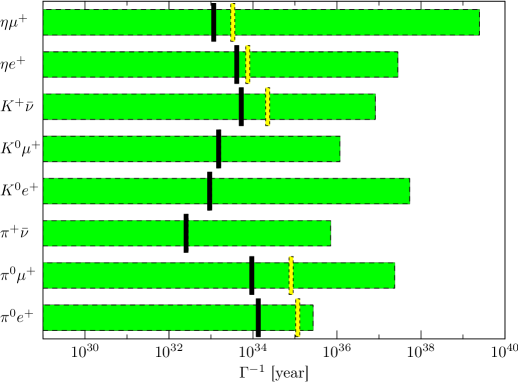
Figure 15: Lifetime of each decay mode induced by the $X$-boson exchange. We take $m_{0}=100$ TeV, $M_{\widetilde{B}}=600$ GeV, $M_{\widetilde{W}}=300$ GeV, $M_{\widetilde{g}}=-2$ TeV, $\mu_{H}=m_{0}$, $M_{X}=10^{16}$ GeV, and $\tan\beta=5$. Black lines represent the Super-Kamiokande constraints at 90 % CL while yellow lines show the future prospects of Hyper-Kamiokande [50, 51].

Now we evaluate the decay lifetime for various modes, which are summarized in the bar chart in Fig. 15. Here, we set the $X$-boson mass to be $M_{X}=10^{16}$ GeV, and other parameters are taken as follows: $m_{0}=100$ TeV, $M_{\widetilde{B}}=600$ GeV, $M_{\widetilde{W}}=300$ GeV, $M_{\widetilde{g}}=-2$ TeV, $\mu_{H}=m_{0}$, and $\tan\beta=5$. From the figure, we see that the decay rates of the modes that contain different generations in their final states are considerably suppressed, as mentioned above. This is because in the $X$-boson exchanging process the CKM is the only source of the flavor violation, which can be seen from Eq. (31). Further, there is no room for the flavor mixing effects in the sfermion mass matrices to modify the decay rates. In this sense, the prediction given here is robust.

4 Summary and Discussion

In this paper, we have studied the impact of the sfermion flavor structure on proton decay in the minimal SUSY SU(5) GUT model. We have found that the flavor violation of the left-handed squark $\delta^{\tilde{Q}}_{13}$ affects the proton decay rates most significantly. The constraint on it from the proton decay bound is stronger than that from the EDMs when the triplet Higgs mass $M_{H_{C}}$ is around $10^{16}$ GeV. Even if $M_{H_{C}}={\cal O}(M_{P})$, $\delta^{\widetilde{Q}}_{13}$ close to unity would be confronted with the current experimental observations.

Other mixing patterns in the left-handed squarks, as well as those in the right-handed up-type squarks also affect the proton decay modes, if these $\delta$’s are close to unity. As for the other sfermion violation, $\delta^{\tilde{L}_{L}}$, $\delta^{\tilde{e}_{R}}$ and $\delta^{\tilde{d}_{R}}$, their impacts are small. In terms of the SU(5) GUT matters, the flavor violation of ${\bf 10}$ matters is to be constrained while that of $\bar{\bf 5}$ is not. This may be consistent with observed large flavor mixing of neutrinos [57].

Further we have found that the flavor violation changes the proton decay branch. The decay pattern of proton reflects the sfermion flavor structure. In particular, the charged lepton modes such as $p\to\pi^{0}\mu^{+}$ may be smoking-gun signature of sfermion flavor violation. Combining indirect probes of sfermion sector via, e.g., the low-energy flavor and EDM measurements [18, 20, 58], gluino decay in collider experiments [19, 59], and observations of gravitational waves [60], we can extract insights to the structure of sfermion sector as well as the underlying GUT model.

We also have discussed possible corrections to the proton decay rates. These corrections are uncertain, unless we clarify the whole picture of the GUT model. This is beyond the scope of this paper and will be done elsewhere [52].

Appendix

Appendix A Input Parameters

Table 1: Physical parameter inputs [31, 61, 62, 63, 64, 65, 66, 67]

$m_{u}^{2{\rm GeV}}$ [MeV]	$m_{d}^{2{\rm GeV}}$ [MeV]	$m_{s}^{2{\rm GeV}}$ [MeV]	$m_{c}(m_{c})$ [GeV]	$m_{b}(m_{b})$ [GeV]
$2.15(15)$	$4.70(20)$	$93.5(2.5)$	$1.275(25)$	$4.18(3)$
$m_{t}^{\rm pole}$ [GeV]	$m_{e}$ [MeV]	$m_{\mu}$ [MeV]	$m_{\tau}$ [MeV]	$a_{3}(m_{Z})^{5}$
$173.24(64)$	0.510998918	105.6583692	$1776.82(16)$	$0.1184(7)$
$m_{h}^{\rm pole}$ [GeV]	$m_{W}$ [GeV]	$m_{Z}$ [GeV]	$(\sqrt{2}G_{\mu})^{-1/2}$ [GeV]
$125.40(45)$	$80.367(7)$	$91.1875(21)$	246.21971
$\sin\theta_{12}$	$\sin\theta_{23}$	$\sin\theta_{13}$	$\delta_{13}$
$0.22535(59)$	$0.04173(57)$	$0.00362(12)$	$1.227(61)$

In this section, we list the set of input parameters which we use in our calculation. The SM parameters are summarized in Table. 1. We take an average of the top mass measured by LHC [61] and Tevatron [62] and the Higgs mass by ATLAS [63] and CMS [64]. We adopt the fitting result of Gfitter [65] as the electroweak gauge boson masses. We use the PDG average of the light quark masses and estimate the Yukawa couplings for the light quarks, by using the four-loop RGEs and three-loop decoupling effects from heavy quarks [68]. Following Ref. [69], we set the weak scale SM parameters.

Table 2: Matrix elements obtained by the lattice simulation in Ref. [48].

Matrix element	Value (GeV2)	Matrix element	Value (GeV2)
$\langle\pi^{0}|(ud)_{R}u_{L}|p\rangle$	$-$0.103(23)(34)	$\langle K^{0}|(us)_{R}u_{L}|p\rangle$	0.098(15)(12)
$\langle\pi^{0}|(ud)_{L}u_{L}|p\rangle$	0.133(29)(28)	$\langle K^{0}|(us)_{L}u_{L}|p\rangle$	0.042(13)(8)
$\langle\pi^{+}|(ud)_{R}d_{L}|p\rangle$	$-$0.146(33)(48)	$\langle K^{+}|(us)_{R}d_{L}|p\rangle$	$-$0.054(11)(9)
$\langle\pi^{+}|(ud)_{L}d_{L}|p\rangle$	0.188(41)(40)	$\langle K^{+}|(us)_{L}d_{L}|p\rangle$	0.036(12)(7)
$\langle\eta^{0}|(ud)_{R}u_{L}|p\rangle$	0.015(14)(17)	$\langle K^{+}|(ud)_{R}s_{L}|p\rangle$	$-$0.093(24)(18)
$\langle\eta^{0}|(ud)_{L}u_{L}|p\rangle$	0.088(21)(16)	$\langle K^{+}|(ud)_{L}s_{L}|p\rangle$	0.111(22)(16)
		$\langle K^{+}|(ds)_{R}u_{L}|p\rangle$	$-$0.044(12)(5)
		$\langle K^{+}|(ds)_{L}u_{L}|p\rangle$	$-$0.076(14)(9)

We also need the hadron matrix elements for the calculation. In Ref. [48], the proton decay matrix elements are evaluated using the direct method with $N_{f}=2+1$ flavor lattice QCD, where $u$ and $d$ quarks are degenerate in mass respecting the isospin symmetry. The results are summarized in Table. 2. In the table, we use an abbreviated notation like

$$\langle\pi^{0}|(ud)_{R}u_{L}|p\rangle=\langle\pi^{0}|\epsilon_{abc}(u^{aT}CP_{R}d^{b})P_{L}u^{c}|p\rangle~{}.$$ (34)

The first and second parentheses represent statistical and systematic errors, respectively. The matrix elements are evaluated at the scale of $\mu=2$ GeV. In the case of the other two combinations of chirality, the matrix elements are derived from the above results through the parity transformation.

Appendix B RGEs of the Wilson Coefficients

In this section, we present the RGEs for the Wilson coefficients of the baryon-number violating operators. First, we give the RGEs of the dimension-five proton decay operators. In this case, since the theory is supersymmetric and the effective operators are written in terms of the superpotential, the renormalization effects are readily obtained from the wave-function renormalization of each chiral superfield in the operators, thanks to the non-renormalization theorem. We derive them at one-loop level as

$$\mu\frac{\partial}{\partial\mu}C^{ijkl}_{5L}(\mu) =\frac{1}{16\pi^{2}}\biggl{[}\bigl{(}-\frac{2}{5}g_{1}^{2}-6g_{2}^{2}-8g_{3}^{2}\bigr{)}C^{ijkl}_{5L}+(f_{u}f_{u}^{\dagger}+f_{d}f_{d}^{\dagger})^{i}_{~{}i^{\prime}}C^{i^{\prime}jkl}_{5L}$$

$$+(f_{u}f_{u}^{\dagger}+f_{d}f_{d}^{\dagger})^{j}_{~{}j^{\prime}}C^{ij^{\prime}kl}_{5L}+(f_{u}f_{u}^{\dagger}+f_{d}f_{d}^{\dagger})^{k}_{~{}k^{\prime}}C^{ijk^{\prime}l}_{5L}+(f_{e}f_{e}^{\dagger})^{l}_{~{}l^{\prime}}C^{ijkl^{\prime}}_{5L}\biggr{]}~{},$$

$$\mu\frac{\partial}{\partial\mu}C^{ijkl}_{5R}(\mu) =\frac{1}{16\pi^{2}}\biggl{[}\bigl{(}-\frac{12}{5}g_{1}^{2}-8g_{3}^{2}\bigr{)}C^{ijkl}_{5R}+C^{i^{\prime}jkl}_{5R}(2f_{u}^{\dagger}f_{u})_{i^{\prime}}^{~{}~{}i}$$

$$+C^{ij^{\prime}kl}_{5R}(2f_{e}^{\dagger}f_{e})_{j^{\prime}}^{~{}~{}j}+C^{ijk^{\prime}l}_{5R}(2f_{u}^{\dagger}f_{u})_{k^{\prime}}^{~{}~{}k}+C^{ijkl^{\prime}}_{5R}(2f_{d}^{\dagger}f_{d})_{l^{\prime}}^{~{}~{}l}\biggr{]}~{}.$$ (35)

Next, we evaluate the RGEs for the coefficients of the four-Fermi operators in Eq. (20). We have [47]

$$\mu\frac{\partial}{\partial\mu}C^{ijkl}_{(1)} =\biggl{[}\frac{\alpha_{1}}{4\pi}\biggl{(}-\frac{11}{10}\biggr{)}+\frac{\alpha_{2}}{4\pi}\biggl{(}-\frac{9}{2}\biggr{)}+\frac{\alpha_{3}}{4\pi}(-4)\biggr{]}C^{ijkl}_{(1)}~{},$$

$$\mu\frac{\partial}{\partial\mu}C^{ijkl}_{(2)} =\biggl{[}\frac{\alpha_{1}}{4\pi}\biggl{(}-\frac{23}{10}\biggr{)}+\frac{\alpha_{2}}{4\pi}\biggl{(}-\frac{9}{2}\biggr{)}+\frac{\alpha_{3}}{4\pi}(-4)\biggr{]}C^{ijkl}_{(2)}~{},$$

$$\mu\frac{\partial}{\partial\mu}C^{ijkl}_{(3)} =\biggl{[}\frac{\alpha_{1}}{4\pi}\biggl{(}-\frac{1}{5}\biggr{)}+\frac{\alpha_{2}}{4\pi}(-3)+\frac{\alpha_{3}}{4\pi}(-4)\biggr{]}C^{ijkl}_{(3)}+\frac{\alpha_{2}}{4\pi}(-4)\bigl{(}C^{jikl}_{(3)}+C^{kjil}_{(3)}+C^{ikjl}_{(3)}\bigr{)}~{},$$

$$\mu\frac{\partial}{\partial\mu}C^{ijkl}_{(4)} =\biggl{[}\frac{\alpha_{1}}{4\pi}\biggl{(}-\frac{6}{5}\biggr{)}+\frac{\alpha_{3}}{4\pi}(-4)\biggr{]}C^{ijkl}_{(4)}+\frac{\alpha_{1}}{4\pi}(-4)C^{kjil}_{(4)}~{}.$$ (36)

Here we neglect the contributions of the Yukawa couplings. In some parameter region, inclusion of the Yukawa interaction changes the proton decay rate by about 10 %. Detailed analysis will be done elsewhere [52].

Finally, we evaluate the long-distance QCD corrections to the baryon-number violating dimension-six operators below the electroweak scale down to the hadronic scale $\mu=2$ GeV. They are calculated at two-loop level in Ref. [70] as

$$\mu\frac{\partial}{\partial\mu}C(\mu)=-\biggl{[}4\frac{\alpha_{s}}{4\pi}+\biggl{(}\frac{14}{3}+\frac{4}{9}N_{f}+\Delta\biggr{)}\frac{\alpha_{s}^{2}}{(4\pi)^{2}}\biggr{]}C(\mu)~{},$$ (37)

where $\alpha_{s}$ is the strong coupling constant, $N_{f}$ denotes the number of quark flavors, and $\Delta=0$ ($\Delta=-10/3$) for $C_{LL}$ ($C_{RL}$). The solution of the equation is

$$\frac{C(\mu)}{C(\mu_{0})}=\biggl{[}\frac{\alpha_{s}(\mu)}{\alpha_{s}(\mu_{0})}\biggr{]}^{-\frac{2}{b_{1}}}\biggl{[}\frac{4\pi b_{1}+b_{2}\alpha_{s}(\mu)}{4\pi b_{1}+b_{2}\alpha_{s}(\mu_{0})}\biggr{]}^{\bigl{(}\frac{2}{b_{1}}-\frac{42+4N_{f}+9\Delta}{18b_{2}}\bigr{)}}~{},$$ (38)

with $b_{1}$ and $b_{2}$ defined by

$$b_{1}=-\frac{11N_{c}-2N_{f}}{3}~{},~{}~{}~{}~{}~{}b_{2}=-\frac{34}{3}N_{c}^{2}+\frac{10}{3}N_{c}N_{f}+2C_{F}N_{f}~{},$$ (39)

where $N_{c}=3$ is the number of colors and $C_{F}$ is the quadratic Casimir invariant defined by $C_{F}\equiv(N_{c}^{2}-1)/{2N_{c}}$. By using the result, we can readily compute the long-distance factor

$$A_{L}\equiv\frac{C(2~{}{\rm GeV})}{C(m_{Z})}~{}$$ (40)

as follows:

$$A_{L}=\biggl{[}\frac{\alpha_{s}(2~{}{\rm GeV})}{\alpha_{s}(m_{b})}\biggr{]}^{\frac{6}{25}}\biggl{[}\frac{\alpha_{s}(m_{b})}{\alpha_{s}(m_{Z})}\biggr{]}^{\frac{6}{23}}\biggl{[}\frac{\alpha_{s}(2~{}{\rm GeV})+\frac{50\pi}{77}}{\alpha_{s}(m_{b})+\frac{50\pi}{77}}\biggr{]}^{-\frac{2047}{11550}}\biggl{[}\frac{\alpha_{s}(m_{b})+\frac{23\pi}{29}}{\alpha_{s}(m_{Z})+\frac{23\pi}{29}}\biggr{]}^{-\frac{1375}{8004}}~{},$$ (41)

for $\Delta=0$, and

$$A_{L}=\biggl{[}\frac{\alpha_{s}(2~{}{\rm GeV})}{\alpha_{s}(m_{b})}\biggr{]}^{\frac{6}{25}}\biggl{[}\frac{\alpha_{s}(m_{b})}{\alpha_{s}(m_{Z})}\biggr{]}^{\frac{6}{23}}\biggl{[}\frac{\alpha_{s}(2~{}{\rm GeV})+\frac{50\pi}{77}}{\alpha_{s}(m_{b})+\frac{50\pi}{77}}\biggr{]}^{-\frac{173}{825}}\biggl{[}\frac{\alpha_{s}(m_{b})+\frac{23\pi}{29}}{\alpha_{s}(m_{Z})+\frac{23\pi}{29}}\biggr{]}^{-\frac{430}{2001}}~{},$$ (42)

for $\Delta=-10/3$. Numerically,

$$A_{L}=\begin{cases}1.257&({\rm for}~{}~{}\Delta=0)\\ 1.253&({\rm for}~{}~{}\Delta=-10/3)\end{cases}~{}.$$ (43)

Appendix C Matching Conditions

Here, we present the matching conditions for the Wilson coefficients.

C.1 At SUSY Breaking Scale

At the sfermion mass scale, the coefficients $C_{5L}^{ijkl}$ and $C_{5R}^{ijkl}$ for the dimension-five operators are matched to those for the four-Fermi operators. The results are given as

$$C^{ijkl}_{(1)}(m_{0}) =C^{ijkl}_{(1)}|_{\widetilde{H}}~{},$$

$$C^{ijkl}_{(2)}(m_{0}) =C^{ijkl}_{(2)}|_{\widetilde{H}}~{},$$

$$C^{ijkl}_{(3)}(m_{0}) =C^{ijkl}_{(3)}|_{\widetilde{g}}+C^{ijkl}_{(3)}|_{\widetilde{W}}+C^{ijkl}_{(3)}|_{\widetilde{B}}~{},$$

$$C^{ijkl}_{(4)}(m_{0}) =C^{ijkl}_{(4)}|_{\widetilde{g}}+C^{ijkl}_{(4)}|_{\widetilde{B}}~{},$$ (44)

where the subscripts $\widetilde{H}$, $\widetilde{g}$, $\widetilde{W}$, and $\widetilde{B}$ represent the contribution of higgsino-, gluino-, wino-, and bino-exchanging diagrams, respectively. They are computed as follows:

$$C^{ijkl}_{(1)}|_{\widetilde{H}} =\frac{1}{(4\pi)^{2}}(2C^{i^{\prime}j^{\prime}kl}_{5L}-C^{ki^{\prime}j^{\prime}l}_{5L}-C^{kj^{\prime}i^{\prime}l}_{5L})F(\mu^{*}_{H},m_{\widetilde{Q}_{I}}^{2},m_{\widetilde{Q}_{J}}^{2})\{(R^{\dagger}_{Q})_{i^{\prime}I}(R_{Q}f^{*}_{u})_{Ii}(R^{\dagger}_{Q})_{j^{\prime}J}(R_{Q}f_{d}^{*})_{Jj}\}$$

$$+\frac{1}{(4\pi)^{2}}(C^{*k^{\prime}l^{\prime}ij}_{5R}-C^{*il^{\prime}k^{\prime}j}_{5R})F(\mu_{H},m_{\widetilde{\bar{u}}_{K}}^{2},m_{\widetilde{\bar{e}}_{L}}^{2})\{(R_{\bar{u}}^{\dagger})_{k^{\prime}K}(R_{\bar{u}}f_{u}^{T})_{Kk}(R_{\bar{e}}^{\dagger})_{l^{\prime}L}(R_{\bar{e}}f_{e}^{T})_{Ll}\}~{},$$

$$C^{ijkl}_{(2)}|_{\widetilde{H}} =\frac{1}{(4\pi)^{2}}(C^{ijk^{\prime}l^{\prime}}_{5L}-C^{k^{\prime}jil^{\prime}}_{5L})F(\mu^{*}_{H},m_{\widetilde{Q}_{K}}^{2},m_{\widetilde{L}_{L}}^{2})\{(R^{\dagger}_{Q})_{k^{\prime}K}(R_{Q}f^{*}_{u})_{Kk}(R_{L}^{\dagger})_{l^{\prime}L}(R_{L}f_{e}^{*})_{Ll}\}$$

$$+\frac{1}{(4\pi)^{2}}(C^{*kli^{\prime}j^{\prime}}_{5R}-C^{*i^{\prime}lkj^{\prime}}_{5R})F(\mu_{H},m_{\widetilde{\bar{u}}_{I}}^{2},m_{\widetilde{\bar{d}}_{J}}^{2})\{(R_{\bar{u}}^{\dagger})_{i^{\prime}I}(R_{\bar{u}}f_{u}^{T})_{Ii}(R_{\bar{d}}^{\dagger})_{j^{\prime}J}(R_{\bar{d}}f_{d}^{T})_{Jj}\}~{}.$$ (45)

$$C_{(3)}^{ijkl}|_{\widetilde{g}}= -\frac{4}{3}\frac{\alpha_{3}}{4\pi}(C^{i^{\prime}j^{\prime}kl}_{5L}-C^{kj^{\prime}i^{\prime}l}_{5L})F(M_{\widetilde{g}},m^{2}_{\widetilde{Q}_{I}},m^{2}_{\widetilde{Q}_{J}})\bigl{\{}(R^{\dagger}_{Q})_{i^{\prime}I}(R_{Q})_{Ii}(R_{Q}^{\dagger})_{j^{\prime}J}(R_{Q})_{Jj}\bigr{\}}~{},$$

$$C_{(4)}^{ijkl}|_{\widetilde{g}}= -\frac{4}{3}\frac{\alpha_{3}}{4\pi}\bigl{[}(C_{5R}^{*i^{\prime}lkj^{\prime}}-C_{5R}^{*kli^{\prime}j^{\prime}})F(M_{\widetilde{g}}^{*},m^{2}_{\widetilde{\bar{u}}_{I}},m^{2}_{\widetilde{\bar{d}}_{J}})\bigl{\{}(R^{\dagger}_{\bar{u}})_{i^{\prime}I}(R_{\bar{u}})_{Ii}(R^{\dagger}_{\bar{d}})_{j^{\prime}J}(R_{\bar{d}})_{Jj}\bigr{\}}$$

$$-(C_{5R}^{*i^{\prime}lk^{\prime}j}-C_{5R}^{*k^{\prime}li^{\prime}j})F(M_{\widetilde{g}}^{*},m^{2}_{\widetilde{\bar{u}}_{I}},m^{2}_{\widetilde{\bar{u}}_{K}})\bigl{\{}(R^{\dagger}_{\bar{u}})_{i^{\prime}I}(R_{\bar{u}})_{Ii}(R^{\dagger}_{\bar{u}})_{k^{\prime}K}(R_{\bar{u}})_{Kk}\bigr{\}}\bigr{]}~{}.$$ (46)

$$C_{(3)}^{ijkl}|_{\widetilde{W}}$$

$$= \frac{\alpha_{2}}{4\pi}F(M_{\widetilde{W}},m^{2}_{\widetilde{Q}_{I}},m^{2}_{\widetilde{Q}_{J}})\bigl{\{}(R^{\dagger}_{Q})_{i^{\prime}I}(R_{Q})_{Ii}(R^{\dagger}_{Q})_{j^{\prime}J}(R_{Q})_{Jj}\bigr{\}}[(C^{i^{\prime}kj^{\prime}l}_{5L}-C^{i^{\prime}j^{\prime}kl}_{5L})+\frac{1}{2}(C^{kj^{\prime}i^{\prime}l}_{5L}-C^{i^{\prime}j^{\prime}kl}_{5L})]$$

$$+ \frac{\alpha_{2}}{4\pi}F(M_{\widetilde{W}},m^{2}_{\widetilde{Q}_{K}},m^{2}_{\widetilde{L}_{L}})\bigl{\{}(R_{Q}^{\dagger})_{k^{\prime}K}(R_{Q})_{Kk}(R^{\dagger}_{L})_{l^{\prime}L}(R_{L})_{Ll}\bigr{\}}[(C^{ik^{\prime}jl^{\prime}}_{5L}-C^{ijk^{\prime}l^{\prime}}_{5L})+\frac{1}{2}(C^{k^{\prime}jil^{\prime}}_{5L}-C^{ijk^{\prime}l^{\prime}}_{5L})]~{}.$$ (47)

$$C_{(3)}^{ijkl}|_{\widetilde{B}} =\frac{6}{5}\frac{\alpha_{1}}{4\pi}[Y_{Q_{L}}Y_{L_{L}}(C^{ijk^{\prime}l^{\prime}}_{5L}-C^{k^{\prime}jil^{\prime}}_{5L})F(M_{\widetilde{B}},m^{2}_{\widetilde{Q}_{K}},m^{2}_{\widetilde{L}_{L}})\bigl{\{}(R_{Q}^{\dagger})_{k^{\prime}K}(R_{Q})_{Kk}(R_{L}^{\dagger})_{l^{\prime}L}(R_{{L}})_{Ll}\bigr{\}}$$

$$+Y_{Q_{L}}^{2}(C^{i^{\prime}j^{\prime}kl}_{5L}-C^{kj^{\prime}i^{\prime}l}_{5L})F(M_{\widetilde{B}},m^{2}_{\widetilde{Q}_{I}},m^{2}_{\widetilde{Q}_{J}})\bigl{\{}(R^{\dagger}_{Q})_{i^{\prime}I}(R_{Q})_{Ii}(R_{Q}^{\dagger})_{j^{\prime}J}(R_{Q})_{Jj}\bigr{\}}]~{},$$

$$C_{(4)}^{ijkl}|_{\widetilde{B}} =-\frac{6}{5}\frac{\alpha_{1}}{4\pi}\bigl{[}Y_{u_{R}}Y_{d_{R}}(C_{5R}^{*kli^{\prime}j^{\prime}}-C_{5R}^{*i^{\prime}lkj^{\prime}})F(M_{\widetilde{B}}^{*},m^{2}_{\widetilde{\bar{u}}_{I}},m^{2}_{\widetilde{\bar{d}}_{J}})\bigl{\{}(R^{\dagger}_{\bar{u}})_{i^{\prime}I}(R_{\bar{u}})_{Ii}(R^{\dagger}_{\bar{d}})_{j^{\prime}J}(R_{\bar{d}})_{Jj}\bigr{\}}$$

$$+Y_{u_{R}}^{2}(C_{5R}^{*i^{\prime}lk^{\prime}j}-C_{5R}^{*k^{\prime}li^{\prime}j})F(M_{\widetilde{B}}^{*},m^{2}_{\widetilde{\bar{u}}_{I}},m^{2}_{\widetilde{\bar{u}}_{K}})\bigl{\{}(R^{\dagger}_{\bar{u}})_{i^{\prime}I}(R_{\bar{u}})_{Ii}(R^{\dagger}_{\bar{u}})_{k^{\prime}K}(R_{\bar{u}})_{Kk}\bigr{\}}$$

$$+Y_{d_{R}}Y_{e_{R}}(C_{5R}^{*il^{\prime}kj^{\prime}}-C_{5R}^{*kl^{\prime}ij^{\prime}})F(M_{\widetilde{B}}^{*},m^{2}_{\widetilde{\bar{d}}_{J}},m^{2}_{\widetilde{\bar{e}}_{L}})\bigl{\{}(R^{\dagger}_{\bar{d}})_{j^{\prime}J}(R_{\bar{d}})_{Jj}(R^{\dagger}_{\bar{e}})_{l^{\prime}L}(R_{\bar{e}})_{Ll}\bigr{\}}$$

$$+Y_{u_{R}}Y_{e_{R}}(C_{5R}^{*k^{\prime}l^{\prime}ij}-C_{5R}^{*il^{\prime}k^{\prime}j})F(M_{\widetilde{B}}^{*},m^{2}_{\widetilde{\bar{u}}_{K}},m^{2}_{\widetilde{\bar{e}}_{L}})\bigl{\{}(R^{\dagger}_{\bar{u}})_{k^{\prime}K}(R_{\bar{u}})_{Kk}(R^{\dagger}_{\bar{e}})_{l^{\prime}L}(R_{\bar{e}})_{Ll}\bigr{\}}\bigr{]}~{}.$$ (48)

Here, $F(M,m_{1}^{2},m_{2}^{2})$ is a loop-function defined by

$$F(M,m_{1}^{2},m_{2}^{2}) \equiv\int\frac{d^{4}q}{\pi^{2}}\frac{iM}{({q}^{2}-M^{2})(q^{2}-m_{1}^{2})(q^{2}-m_{2}^{2})}~{},$$

$$=\frac{M}{m_{1}^{2}-m_{2}^{2}}\biggl{[}\frac{m_{1}^{2}}{m_{1}^{2}-M^{2}}\ln\biggl{(}\frac{m_{1}^{2}}{M^{2}}\biggr{)}-\frac{m_{2}^{2}}{m_{2}^{2}-M^{2}}\ln\biggl{(}\frac{m_{2}^{2}}{M^{2}}\biggr{)}\biggr{]}~{}.$$ (49)

The matrices $R_{f}$ ($f=Q,L,\bar{u},\bar{d},\bar{e}$) are unitary matrices which diagonalize the corresponding sfermion mass matrices; for instance,

$$R_{Q}~{}m_{\widetilde{Q}_{L}}^{2}R_{Q}^{\dagger} ={\rm diag}(m^{2}_{\widetilde{Q}_{1}},m^{2}_{\widetilde{Q}_{2}},m^{2}_{\widetilde{Q}_{3}})~{},$$

$$R_{\bar{u}}(m_{\widetilde{\bar{u}}_{R}}^{2})^{t}R_{\bar{u}}^{\dagger} ={\rm diag}(m^{2}_{\widetilde{\bar{u}}_{1}},m^{2}_{\widetilde{\bar{u}}_{2}},m^{2}_{\widetilde{\bar{u}}_{3}})~{},$$ (50)

and so on. In the calculation, we ignore the terms suppressed by $v/m_{0}$ ($v$ is the VEV of the Higgs field) such as the left-right mixing terms in sfermion mass matrices.

From the above expression, it is found that in the limit of degenerate squark masses or no flavor-mixing, the coefficients $C_{(3)}^{ijkl}|_{\widetilde{g}}$ vanish; they become proportional to $(C^{ijkl}_{5L}-C^{kjil}_{5L})$, and thus

$$C_{(3)}^{ijkl}|_{\widetilde{g}}{\cal O}^{(3)}_{ijkl} \propto(C^{ijkl}_{5L}-C^{kjil}_{5L}){\cal O}^{(3)}_{ijkl}=\frac{1}{2}C^{ijkl}_{5L}\bigl{\{}{\cal O}^{(3)}_{ijkl}+{\cal O}^{(3)}_{jikl}-{\cal O}^{(3)}_{kijl}-{\cal O}^{(3)}_{kjil}\bigr{\}}=0~{}.$$ (51)

The last equality immediately follows from the identity

$$\epsilon^{\alpha\beta}\epsilon^{\gamma\delta}-\epsilon^{\gamma\beta}\epsilon^{\alpha\delta}+\epsilon^{\alpha\gamma}\epsilon^{\delta\beta}=0~{},$$ (52)

and the Fierz identities.

In the case of $C_{(4)}^{ijkl}|_{\widetilde{g}}$, they again vanish in the degenerate mass limit. On the other hand, they may not vanish when there is no flavor-mixing in squark mass matrices; in this case,

$$C_{(4)}^{ijkl}|_{\widetilde{g}}\propto(C^{*ilkj}_{5R}-C^{*klij}_{5R})[F(M_{\widetilde{g}},m^{2}_{\widetilde{\bar{u}}_{i}},m^{2}_{\widetilde{\bar{d}}_{j}})-F(M_{\widetilde{g}},m^{2}_{\widetilde{\bar{u}}_{i}},m^{2}_{\widetilde{\bar{u}}_{k}})]~{},$$ (53)

and thus they can remain sizable when there exists mass difference among right-handed squarks. Their contribution to the proton decay rate turns out to be negligible, though. Since charm quark is heavier than proton, all we have to consider is the $i=k=1$ components, which prove to be zero as one can see from the above expression. Similar arguments can be applied to the case of the bino and neutral-wino contributions. As a result, one can find that it is the charged wino and higgsino contribution that does remain in this limit.

C.2 At Electroweak Scale

Next, we give the matching conditions for the Wilson coefficients $C_{RL}$ and $C_{LL}$ in Eq. (21) at the electroweak scale $\mu=m_{Z}$. The result is

$$C_{RL}(dsu\nu_{i}) =0~{},$$

$$C_{RL}(usd\nu_{i}) =-(V_{\rm CKM})_{j1}C^{12ji}_{(1)}(m_{Z})~{},$$

$$C_{RL}(uds\nu_{i}) =-(V_{\rm CKM})_{j2}C^{11ji}_{(1)}(m_{Z})~{},$$

$$C_{LL}(dsu\nu_{i}) =(V_{\rm CKM})_{j1}(V_{\rm CKM})_{k2}[C^{jk1i}_{(3)}(m_{Z})-C^{kj1i}_{(3)}(m_{Z})]~{},$$

$$C_{LL}(usd\nu_{i}) =(V_{\rm CKM})_{j1}(V_{\rm CKM})_{k2}C^{k1ji}_{(3)}(m_{Z})~{},$$

$$C_{LL}(uds\nu_{i}) =(V_{\rm CKM})_{j1}(V_{\rm CKM})_{k2}C^{j1ki}_{(3)}(m_{Z})~{}.$$ (54)

From the equations, it is found that only the operators ${\cal O}^{(1)}_{ijkl}$ and ${\cal O}^{(3)}_{ijkl}$ contribute to the $p\to K^{+}\bar{\nu}$ mode.

Appendix D Partial Decay Width

Here, we summarize the expressions for other decay modes than the $p\to K^{+}\bar{\nu}$ mode described in the text.

D.1 Kaon and Charged Lepton

The effective Lagrangian which induces the $p\to K^{0}l^{+}_{i}$ ($l^{+}_{i}=e^{+},\mu^{+}$) mode is given as

$${\cal L}(p\to K^{0}l^{+}_{i}) =C_{RL}(usul_{i})\bigl{[}\epsilon_{abc}(u_{R}^{a}s_{R}^{b})(u_{L}^{c}l_{Li})\bigr{]}+C_{LL}(usul_{i})\bigl{[}\epsilon_{abc}(u_{L}^{a}s_{L}^{b})(u_{L}^{c}l_{Li})\bigr{]}$$

$$+C_{LR}(usul_{i})\bigl{[}\epsilon_{abc}(u_{L}^{a}s_{L}^{b})(u_{R}^{c}l_{Ri})\bigr{]}+C_{RR}(usul_{i})\bigl{[}\epsilon_{abc}(u_{R}^{a}s_{R}^{b})(u_{R}^{c}l_{Ri})\bigr{]}~{}.$$ (55)

The matching condition for the Wilson coefficients is

$$C_{RL}(usul_{i}) =C^{121i}_{(1)}(m_{Z})~{},$$

$$C_{LR}(usul_{i}) =(V_{\rm CKM})_{j2}[C^{1j1i}_{(2)}(m_{Z})+C^{j11i}_{(2)}(m_{Z})]~{},$$

$$C_{LL}(usul_{i}) =-(V_{\rm CKM})_{j2}C^{1j1i}_{(3)}(m_{Z})~{},$$

$$C_{RR}(usul_{i}) =C^{121i}_{(4)}(m_{Z})~{}.$$ (56)

Then, we obtain the partial decay width as

$$\Gamma(p\to K^{0}l^{+}_{i})=\frac{m_{p}}{32\pi}\biggl{(}1-\frac{m_{K}^{2}}{m_{p}^{2}}\biggr{)}^{2}\bigl{[}|{\cal A}_{L}(p\to K^{0}l^{+}_{i})|^{2}+|{\cal A}_{R}(p\to K^{0}l^{+}_{i})|^{2}\bigr{]}~{},$$ (57)

where

$${\cal A}_{L}(p\to K^{0}l^{+}_{i}) =C_{RL}(usul_{i})\langle K^{0}|(us)_{R}u_{L}|p\rangle+C_{LL}(usul_{i})\langle K^{0}|(us)_{L}u_{L}|p\rangle~{},$$

$${\cal A}_{R}(p\to K^{0}l^{+}_{i}) =C_{LR}(usul_{i})\langle K^{0}|(us)_{R}u_{L}|p\rangle+C_{RR}(usul_{i})\langle K^{0}|(us)_{L}u_{L}|p\rangle~{}.$$ (58)

Notice that we have used the parity transformation to obtain the hadron matrix elements for ${\cal A}_{R}$.

D.2 Pion and Anti-neutrino

For the $p\to\pi^{+}\bar{\nu}_{i}$ modes, the effective Lagrangian is given as

$${\cal L}(p\to\pi^{+}\bar{\nu}_{i}) =C_{RL}(udd\nu_{i})\bigl{[}\epsilon_{abc}(u_{R}^{a}d_{R}^{b})(d_{L}^{c}\nu_{Li})\bigr{]}+C_{LL}(udd\nu_{i})\bigl{[}\epsilon_{abc}(u_{L}^{a}d_{L}^{b})(d_{L}^{c}\nu_{Li})\bigr{]}~{},$$ (59)

and the matching condition for the Wilson coefficients is

$$C_{RL}(udd\nu_{i}) =-(V_{\rm CKM})_{j1}C^{11ji}_{(1)}~{},$$

$$C_{LL}(udd\nu_{i}) =(V_{\rm CKM})_{j1}(V_{\rm CKM})_{k1}C^{j1ki}_{(3)}~{}.$$ (60)

The partial decay width is then computed as

$$\Gamma(p\to\pi^{+}\bar{\nu}_{i})=\frac{m_{p}}{32\pi}\biggl{(}1-\frac{m_{\pi}^{2}}{m_{p}^{2}}\biggr{)}^{2}|{\cal A}(p\to\pi^{+}\bar{\nu}_{i})|^{2}~{},$$ (61)

where

$${\cal A}_{L}(p\to\pi^{+}\bar{\nu}_{i}) =C_{RL}(udd\nu_{i})\langle\pi^{+}|(ud)_{R}d_{L}|p\rangle+C_{LL}(udd\nu_{i})\langle\pi^{+}|(ud)_{L}d_{L}|p\rangle~{}.$$ (62)

D.3 Pion/eta and Charged Lepton

The effective Lagrangian for the $p\to\pi^{0}l^{+}_{i}$ is

$${\cal L}(p\to\pi^{0}l^{+}_{i}) =C_{RL}(udul_{i})\bigl{[}\epsilon_{abc}(u_{R}^{a}d_{R}^{b})(u_{L}^{c}l_{Li})\bigr{]}+C_{LL}(udul_{i})\bigl{[}\epsilon_{abc}(u_{L}^{a}d_{L}^{b})(u_{L}^{c}l_{Li})\bigr{]}$$

$$+C_{LR}(udul_{i})\bigl{[}\epsilon_{abc}(u_{L}^{a}d_{L}^{b})(u_{R}^{c}l_{Ri})\bigr{]}+C_{RR}(udul_{i})\bigl{[}\epsilon_{abc}(u_{R}^{a}d_{R}^{b})(u_{R}^{c}l_{Ri})\bigr{]}~{}.$$ (63)

We have the matching condition for the Wilson coefficients at the electroweak scale as

$$C_{RL}(udul_{i}) =C^{111i}_{(1)}(m_{Z})~{},$$

$$C_{LR}(udul_{i}) =(V_{\rm CKM})_{j1}[C^{1j1i}_{(2)}(m_{Z})+C^{j11i}_{(2)}(m_{Z})]~{},$$

$$C_{LL}(udul_{i}) =-(V_{\rm CKM})_{j1}C^{1j1i}_{(3)}(m_{Z})~{},$$

$$C_{RR}(udul_{i}) =C^{111i}_{(4)}(m_{Z})~{}.$$ (64)

With the coefficients, the partial decay width is expressed as

$$\Gamma(p\to\pi^{0}l^{+}_{i})=\frac{m_{p}}{32\pi}\biggl{(}1-\frac{m_{\pi}^{2}}{m_{p}^{2}}\biggr{)}^{2}\bigl{[}|{\cal A}_{L}(p\to\pi^{0}l^{+}_{i})|^{2}+|{\cal A}_{R}(p\to\pi^{0}l^{+}_{i})|^{2}\bigr{]}~{},$$ (65)

where

$${\cal A}_{L}(p\to\pi^{0}l^{+}_{i}) =C_{RL}(udul_{i})\langle\pi^{0}|(ud)_{R}u_{L}|p\rangle+C_{LL}(udul_{i})\langle\pi^{0}|(ud)_{L}u_{L}|p\rangle~{},$$

$${\cal A}_{R}(p\to\pi^{0}l^{+}_{i}) =C_{LR}(udul_{i})\langle\pi^{0}|(ud)_{R}u_{L}|p\rangle+C_{RR}(udul_{i})\langle\pi^{0}|(ud)_{L}u_{L}|p\rangle~{}.$$ (66)

The same interaction also induces the $p\to\eta^{0}l_{i}^{+}$ modes. In this case we have

$$\Gamma(p\to\eta^{0}l^{+}_{i})=\frac{m_{p}}{32\pi}\biggl{(}1-\frac{m_{\eta}^{2}}{m_{p}^{2}}\biggr{)}^{2}\bigl{[}|{\cal A}_{L}(p\to\eta^{0}l^{+}_{i})|^{2}+|{\cal A}_{R}(p\to\eta^{0}l^{+}_{i})|^{2}\bigr{]}~{},$$ (67)

with

$${\cal A}_{L}(p\to\eta^{0}l^{+}_{i}) =C_{RL}(udul_{i})\langle\eta^{0}|(ud)_{R}u_{L}|p\rangle+C_{LL}(udul_{i})\langle\eta^{0}|(ud)_{L}u_{L}|p\rangle~{},$$

$${\cal A}_{R}(p\to\eta^{0}l^{+}_{i}) =C_{LR}(udul_{i})\langle\eta^{0}|(ud)_{R}u_{L}|p\rangle+C_{RR}(udul_{i})\langle\eta^{0}|(ud)_{L}u_{L}|p\rangle~{}.$$ (68)

References

- [1] J. D. Wells, [hep-ph/0306127].
- [2] N. Arkani-Hamed and S. Dimopoulos, JHEP 0506, 073 (2005) [hep-th/0405159].
- [3] G. F. Giudice and A. Romanino, Nucl. Phys. B 699, 65 (2004) [Erratum-ibid. B 706, 65 (2005)] [hep-ph/0406088].
- [4] N. Arkani-Hamed, S. Dimopoulos, G. F. Giudice and A. Romanino, Nucl. Phys. B 709, 3 (2005) [hep-ph/0409232].
- [5] J. D. Wells, Phys. Rev. D 71, 015013 (2005) [hep-ph/0411041].
-
[6]
G. Aad et al. [ATLAS Collaboration],
Phys. Lett. B 716, 1 (2012)
[arXiv:1207.7214]. -
[7]
S. Chatrchyan et al. [CMS Collaboration],
Phys. Lett. B 716, 30 (2012)
[arXiv:1207.7235]. - [8] Y. Okada, M. Yamaguchi and T. Yanagida, Prog. Theor. Phys. 85, 1 (1991); Y. Okada, M. Yamaguchi and T. Yanagida, Phys. Lett. B 262, 54 (1991); J. R. Ellis, G. Ridolfi and F. Zwirner, Phys. Lett. B 257, 83 (1991); H. E. Haber and R. Hempfling, Phys. Rev. Lett. 66, 1815 (1991); J. R. Ellis, G. Ridolfi and F. Zwirner, Phys. Lett. B 262, 477 (1991).
- [9] G. F. Giudice and A. Strumia, Nucl. Phys. B 858, 63 (2012) [arXiv:1108.6077].
- [10] L. J. Hall and Y. Nomura, JHEP 1201, 082 (2012) [arXiv:1111.4519]; L. J. Hall, Y. Nomura and S. Shirai, JHEP 1301, 036 (2013) [arXiv:1210.2395].
- [11] M. Ibe and T. T. Yanagida, Phys. Lett. B 709, 374 (2012) [arXiv:1112.2462]; M. Ibe, S. Matsumoto and T. T. Yanagida, Phys. Rev. D 85, 095011 (2012) [arXiv:1202.2253].
-
[12]
A. Arvanitaki, N. Craig, S. Dimopoulos and G. Villadoro,
JHEP 1302, 126 (2013)
[arXiv:1210.0555]. -
[13]
N. Arkani-Hamed, A. Gupta, D. E. Kaplan, N. Weiner and T. Zorawski,
[arXiv:1212.6971]. -
[14]
J. Hisano, T. Kuwahara and N. Nagata,
Phys. Lett. B 723, 324 (2013)
[arXiv:1304.0343]. - [15] H. Murayama and A. Pierce, Phys. Rev. D 65, 055009 (2002) [hep-ph/0108104].
-
[16]
J. Hisano, D. Kobayashi, T. Kuwahara and N. Nagata,
JHEP 1307, 038 (2013)
[arXiv:1304.3651]. - [17] M. Dine, P. Draper and W. Shepherd, [arXiv:1308.0274].
-
[18]
D. McKeen, M. Pospelov and A. Ritz,
Phys. Rev. D 87, 113002 (2013)
[arXiv:1303.1172]. - [19] R. Sato, S. Shirai and K. Tobioka, JHEP 1310, 157 (2013) [arXiv:1307.7144].
-
[20]
W. Altmannshofer, R. Harnik and J. Zupan,
JHEP 1311, 202 (2013)
[arXiv:1308.3653]. - [21] G. F. Giudice and A. Masiero, Phys. Lett. B 206, 480 (1988).
- [22] K. Inoue, M. Kawasaki, M. Yamaguchi and T. Yanagida, Phys. Rev. D 45, 328 (1992).
- [23] J. A. Casas and C. Munoz, Phys. Lett. B 306, 288 (1993) [hep-ph/9302227].
- [24] G. F. Giudice, M. A. Luty, H. Murayama and R. Rattazzi, JHEP 9812, 027 (1998) [hep-ph/9810442]; L. Randall and R. Sundrum, Nucl. Phys. B 557, 79 (1999) [hep-th/9810155]; M. Dine and D. MacIntire, Phys. Rev. D 46, 2594 (1992) [hep-ph/9205227]; J. A. Bagger, T. Moroi and E. Poppitz, JHEP 0004, 009 (2000) [hep-th/9911029]; P. Binetruy, M. K. Gaillard and B. D. Nelson, Nucl. Phys. B 604, 32 (2001) [hep-ph/0011081].
- [25] D. M. Pierce, J. A. Bagger, K. T. Matchev and R. j. Zhang, Nucl. Phys. B 491, 3 (1997) [hep-ph/9606211].
-
[26]
K. Nakayama and T. T. Yanagida,
Phys. Lett. B 722, 107 (2013)
[arXiv:1302.3332]. -
[27]
K. Harigaya, M. Ibe and T. T. Yanagida,
JHEP 1312, 016 (2013)
[arXiv:1310.0643]. - [28] F. Gabbiani, E. Gabrielli, A. Masiero and L. Silvestrini, Nucl. Phys. B 477 (1996) 321 [hep-ph/9604387].
- [29] M. Bona et al. [UTfit Collaboration], JHEP 0803, 049 (2008) [arXiv:0707.0636].
-
[30]
A. J. Bevan et al. [UTfit Collaboration],
JHEP 1210, 068 (2012)
[arXiv:1206.6245]. - [31] http://www.utfit.org/UTfit/ResultsSummer2013PostEPS
- [32] R. D. Peccei and H. R. Quinn, Phys. Rev. Lett. 38, 1440 (1977).
- [33] S. Weinberg, Phys. Rev. Lett. 63, 2333 (1989).
-
[34]
G. Degrassi, E. Franco, S. Marchetti and L. Silvestrini,
JHEP 0511, 044 (2005)
[hep-ph/0510137]. -
[35]
K. Fuyuto, J. Hisano, N. Nagata and K. Tsumura,
JHEP 1312, 010 (2013)
[arXiv:1308.6493]. -
[36]
C. A. Baker, D. D. Doyle, P. Geltenbort, K. Green, M. G. D. van der
Grinten, P. G. Harris, P. Iaydjiev and S. N. Ivanov et al.,
Phys. Rev. Lett. 97, 131801 (2006)
[hep-ex/0602020]. -
[37]
J. Hisano, J. Y. Lee, N. Nagata and Y. Shimizu,
Phys. Rev. D 85, 114044 (2012)
[arXiv:1204.2653]. -
[38]
K. Fuyuto, J. Hisano and N. Nagata,
Phys. Rev. D 87, 054018 (2013)
[arXiv:1211.5228]. - [39] S. Dimopoulos and H. Georgi, Nucl. Phys. B 193, 150 (1981).
- [40] N. Sakai, Z. Phys. C 11, 153 (1981).
- [41] H. Georgi and S. L. Glashow, Phys. Rev. Lett. 32, 438 (1974).
- [42] J. R. Ellis, M. K. Gaillard and D. V. Nanopoulos, Phys. Lett. B 88, 320 (1979).
- [43] N. Sakai and T. Yanagida, Nucl. Phys. B 197, 533 (1982).
- [44] S. Weinberg, Phys. Rev. D 26, 287 (1982).
- [45] S. Weinberg, Phys. Rev. Lett. 43, 1566 (1979).
- [46] F. Wilczek and A. Zee, Phys. Rev. Lett. 43, 1571 (1979).
- [47] L. F. Abbott and M. B. Wise, Phys. Rev. D 22, 2208 (1980).
- [48] Y. Aoki, E. Shintani and A. Soni, [arXiv:1304.7424].
- [49] T. Goto and T. Nihei, Phys. Rev. D 59, 115009 (1999) [hep-ph/9808255].
- [50] M. Shiozawa, talk presented at TAUP 2013, September 8--13, Asilomar, CA, USA.
-
[51]
K. S. Babu, E. Kearns, U. Al-Binni, S. Banerjee, D. V. Baxter,
Z. Berezhiani, M. Bergevin and S. Bhattacharya et al.,
Baryon Number Violation,
[arXiv:1311.5285]. - [52] N. Nagata and S. Shirai, in preparation.
- [53] N. Sakai, Phys. Lett. B 121, 130 (1983).
- [54] N. Haba and N. Okada, Europhys. Lett. 82, 61001 (2008) [hep-ph/0601003].
- [55] E. Cremmer, B. Julia, J. Scherk, S. Ferrara, L. Girardello and P. van Nieuwenhuizen, Nucl. Phys. B 147, 105 (1979); E. Cremmer, S. Ferrara, L. Girardello and A. Van Proeyen, Nucl. Phys. B 212, 413 (1983); T. Kugo and S. Uehara, Nucl. Phys. B 222, 125 (1983); T. Kugo and S. Uehara, Nucl. Phys. B 226, 49 (1983).
- [56] J. Hisano, D. Kobayashi, Y. Muramatsu and N. Nagata, Phys. Lett. B 724, 283 (2013) [arXiv:1302.2194].
-
[57]
L. J. Hall, H. Murayama and N. Weiner,
Phys. Rev. Lett. 84, 2572 (2000)
[hep-ph/9911341]. - [58] T. Moroi and M. Nagai, Phys. Lett. B 723, 107 (2013) [arXiv:1303.0668]; T. Moroi, M. Nagai and T. T. Yanagida, [arXiv:1305.7357].
- [59] R. Sato, S. Shirai and K. Tobioka, JHEP 1211, 041 (2012) [arXiv:1207.3608].
- [60] R. Saito and S. Shirai, Phys. Lett. B 713, 237 (2012) [arXiv:1201.6589].
- [61] The ATLAS collaboration, ATLAS-CONF-2013-102.
- [62] M. Muether [Tevatron Electroweak Working Group and CDF and D0 Collaborations], [arXiv:1305.3929].
- [63] [ATLAS Collaboration], ATLAS-CONF-2013-014.
-
[64]
S. Chatrchyan et al. [CMS Collaboration],
JHEP 1306, 081 (2013)
[arXiv:1303.4571]. - [65] M. Baak and R. Kogler, [arXiv:1306.0571].
- [66] J. Beringer et al. [Particle Data Group Collaboration], Phys. Rev. D 86, 010001 (2012).
- [67] S. Bethke, Nucl. Phys. Proc. Suppl. 234, 229 (2013) [arXiv:1210.0325].
-
[68]
K. G. Chetyrkin, B. A. Kniehl and M. Steinhauser,
Phys. Rev. Lett. 79, 2184 (1997)
[hep-ph/9706430]. - [69] D. Buttazzo, G. Degrassi, P. P. Giardino, G. F. Giudice, F. Sala, A. Salvio and A. Strumia, JHEP 1312, 089 (2013) [arXiv:1307.3536].
- [70] T. Nihei and J. Arafune, Prog. Theor. Phys. 93, 665 (1995) [hep-ph/9412325].