Sparse graphs using exchangeable random measures

Abstract

Statistical network modeling has focused on representing the graph as a discrete structure, namely the adjacency matrix, and considering the exchangeability of this array. In such cases, the Aldous-Hoover representation theorem (Aldous, 1981; Hoover, 1979) applies and informs us that the graph is necessarily either dense or empty. In this paper, we instead consider representing the graph as a measure on $\mathbb{R}_{+}^{2}$. For the associated definition of exchangeability in this continuous space, we rely on the Kallenberg representation theorem (Kallenberg, 2005). We show that for certain choices of such exchangeable random measures underlying our graph construction, our network process is sparse with power-law degree distribution. In particular, we build on the framework of completely random measures (CRMs) and use the theory associated with such processes to derive important network properties, such as an urn representation for our analysis and network simulation. Our theoretical results are explored empirically and compared to common network models. We then present a Hamiltonian Monte Carlo algorithm for efficient exploration of the posterior distribution and demonstrate that we are able to recover graphs ranging from dense to sparse—and perform associated tests—based on our flexible CRM-based formulation. We explore network properties in a range of real datasets, including Facebook social circles, a political blogosphere, protein networks, citation networks, and world wide web networks, including networks with hundreds of thousands of nodes and millions of edges.

1401.1137

and

t1FC acknowledges the support of the European Commission under the Marie Curie Intra-European Fellowship Programme. t2EBF was supported in part by DARPA Grant FA9550-12-1-0406 negotiated by AFOSR and AFOSR Grant FA9550-12-1-0453.

1 Introduction

The rapid increase in the availability and importance of network data has been a driving force behind the significant recent attention on random graph models. This effort builds on a long history, with a popular early model being the Erdös Rényi random graph (Erdös and Rényi, 1959). However, the Erdös Rényi formulation has since been dismissed as overly simplistic since it fails to capture important real-world network properties. A plethora of other network models have been proposed in recent years, with some overviews of such models provided in (Newman, 2003, 2009; Bollobás, 2001; Durrett, 2007; Goldenberg et al., 2010; Fienberg, 2012).

In many scenarios, it is appealing conceptually to assume that the order in which nodes are observed is of no importance (Bickel and Chen, 2009; Hoff, 2009). In statistical network models, this equates with the notion of exchangeability. Classically, the graph has been represented by a discrete structure, or adjacency matrix, $Z$ where $Z_{ij}$ is a binary variable with $Z_{ij}=1$ indicating an edge from node $i$ to node $j$. In the case of undirected graphs, we furthermore restrict $Z_{ij}=Z_{ji}$. For generic matrices $Z$ in some space $\mathbf{Z}$, an (infinite) exchangeable random array (Diaconis and Janson, 2008; Lauritzen, 2008) is one such that

$$(Z_{ij})\overset{d}{=}(Z_{\pi(i)\sigma(j)})\text{ for }(i,j)\in\mathbb{N}^{2}$$ (1)

for any permutation $\pi,\sigma$ of $\mathbb{N}$, with $\pi=\sigma$ in the jointly exchangeable case.

The celebrated Aldous-Hoover theorem (Aldous, 1981; Hoover, 1979) states that infinite exchangeability implies a mixture model representation for the matrix involving transformations of uniform random variables (see Theorem 1). For undirected graphs, this transformation is specified by the graphon.

The Aldous-Hoover constructive definition has motivated the development of Bayesian statistical models for arrays (Lloyd et al., 2012) and many popular network models can be recast in this framework (Hoff, Raftery and Handcock, 2002; Nowicki and Snijders, 2001; Airoldi et al., 2008; Kim and Leskovec, 2012; Miller, Griffiths and Jordan, 2009). Estimators of models in this class and their associated properties have been studied extensively in recent years (Bickel and Chen, 2009; Bickel, Chen and Levina, 2011; Rohe, Chatterjee and Yu, 2011; Zhao, Levina and Zhu, 2012; Airoldi, Costa and Chan, 2014; Wolfe and Choi, 2014).

However, one unpleasing consequence of the Aldous-Hoover theorem is that graphs represented by an exchangeable random array are either trivially empty or dense, i.e. the number of edges grows quadratically with the number of nodes $n$ (see Theorem B.18). To quote the survey of Orbanz and Roy (2015) “the theory also clarifies the limitations of exchangeable models. It shows, for example, that most Bayesian models of network data are inherently misspecified.” The conclusion is that we cannot have both exchangeability of the nodes (in the sense of (1)), a cornerstone of Bayesian modeling, and sparse graphs, which is what we observe in the real world (Newman, 2009), especially for large networks. Several models have been developed which give up exchangeability in order to obtain sparse graphs (Barabási and Albert, 1999). Alternatively, there is a body of literature that examines rescaling graph properties with network size $n$, leading to sparse graph sequences where each graph is finitely exchangeable (Bollobás, Janson and Riordan, 2007; Bollobás and Riordan, 2009; Wolfe and Olhede, 2013; Borgs et al., 2014). However, any method building on a rescaling-based approach provides a graph distribution, $\pi_{n}$, that lacks projectivity: marginalizing node $n$ does not yield $\pi_{n-1}$, the distribution on graphs of size $n-1$.

Figure 1: Point process representation of a random graph. Each node $i$ is embedded in $\mathbb{R}_{+}$ at some location $\theta_{i}$ and is associated with a sociability parameter $w_{i}$. An edge between nodes $\theta_{i}$ and $\theta_{j}$ is represented by a point at locations $(\theta_{i},\theta_{j})$ and $(\theta_{j},\theta_{i})$ in $\mathbb{R}_{+}^{2}$.

To leverage some of the benefits of generative exchangeable modeling while producing sparse graphs with power-law behavior, we set aside the discrete array structure of the adjacency matrix and instead consider a different notion of exchangeability of a continuous-space representation of networks based on a point process on $\mathbb{R}_{+}^{2}$ (see Figure 1)

$$Z=\sum_{i,j}z_{ij}\delta_{(\theta_{i},\theta_{j})},$$ (2)

where $z_{ij}=1$ if there is a link between nodes $\theta_{i}$ and $\theta_{j}$ in $\mathbb{R}_{+}$, and is 0 otherwise. Our notion of exchangeability in this framework is as follows. Paralleling (1), the point process $Z$ on $\mathbb{R}_{+}^{2}$ is exchangeable if and only if, for any $h>0$ and for any permutations $\pi,\sigma$ of $\mathbb{N}$,

$$(Z(A_{i}\times A_{j}))\overset{d}{=}(Z(A_{\pi(i)}\times A_{\sigma(j)}))\text{ for }(i,j)\in\mathbb{N}^{2},$$ (3)

where here we consider intervals $A_{i}=[h(i-1),hi]$ with $i\in\mathbb{N}$. Considering arbitrarily small intervals $A_{i}$, such that two nodes $\theta_{j}$ and $\theta_{k}$ are unlikely to fall into the same interval, leads to a similar intuition and statistical implication of exchangeability as in the Aldous-Hoover framework. Note, however, that if we order nodes in (2) by the first time an edge appears for that node, and look at the associated adjacency matrix, then this array is not exchangeable in the sense of (1). Importantly, though, our notion of exchangeability allows us to define a practical and efficient inference algorithm (described in Section 6) due to the invariance property in the continuous space specified in (3).

In place of the Aldous-Hoover theorem, we now appeal to the continuous-space counterpart (Kallenberg, 2005, Chapter 9) which provides a representation theorem for exchangeable point processes on $\mathbb{R}_{+}^{2}$: a point process is exchangeable if and only if it can be represented as a transformation of unit-rate Poisson processes and uniform random variables (see Theorem 2); this is in direct analogy to the graphon transformation of uniform random variables in the Aldous-Hoover representation. More precisely, within the Kallenberg framework, we consider that two nodes $i\neq j$ connect with probability

$$\Pr(z_{ij}=1|w_{i},w_{j})=1-e^{-2w_{i}w_{j}}$$ (4)

where the positive sociability parameters $(w_{i})_{i=1,2,\ldots}$ are the points of a Poisson point process, or equivalently the jumps of a completely random measure (CRM) (Kingman, 1967, 1993; Lijoi and Prünster, 2010). We show that by carefully choosing the Lévy measure characterizing this CRM, we are able to construct graphs ranging from sparse to dense. In particular, any Lévy measure yielding an infinite activity CRM leads to sparse graphs; alternatively, finite activity CRMs, whose associated point processes are in the compound Poisson process family, yield dense graphs. When building on a specific class of infinite activity regularly varying CRMs, we can obtain graphs where the number of edges increases at a rate below $n^{a}$ for some constant $1<a<2$ that depends on the Lévy measure. The associated degree distribution has a power-law form.

By building on the framework of CRMs, we are able to harness the considerable theory and practicality of such processes to (1) derive important properties of our proposed model and (2) develop an efficient statistical estimation procedure. The CRM construction enables us to relate the sparsity properties of the graph to the properties of the Lévy measure. We also utilize the CRM-based formulation to develop a scalable Hamiltonian Monte Carlo sampler that can automatically handle a range of graphs from dense to sparse based on inferring a graph sparsity parameter. We show in Section 7 that our methods scale to graphs with hundreds of thousands of nodes and millions of edges. Thus, our generative specification enjoys both an analytic representation in the Kallenberg framework and a formulation in terms of CRMs. The former allows us to nicely connect with existing random graph models whereas the latter provides (1) connections to the Bayesian nonparametric modeling and inference literature and (2) interpretability and theoretical analysis of the formulation.

In summary, our proposed framework captures a number of desirable properties:

• Sparsity. We can obtain graphs where the number of edges increases sub-quadratically with the number of nodes.

• Power Law. Our formulation yields a power-law form, which is useful in modeling many real-world graphs (Newman, 2009).

• Exchangeability in the sense of (3).

• Simplicity. Three hyperparameters tune the expected number of nodes, power-law properties, etc.

• Interpretability. The node-specific sociability parameters, $w_{i}$, lead to straightforward interpretability of the model.

• Scalable inference. Our CRM-based Hamiltonian Monte Carlo sampler efficiently scales to large, real-world graphs, allowing for rapid analysis of graph properties such as sparsity, power-law, etc.

A bipartite random graph formulation with power-law behavior building on CRMs was first proposed by Caron (2012). In this paper, we consider a more general CRM-based framework for bipartite graphs, directed multigraphs, and undirected graphs. More importantly, we prove that the resulting formulation yields sparse graphs under certain conditions—a notion not explored in (Caron, 2012)—and cast exchangeability within the Kallenberg representation theorem. Both of these represent important and non-trivial extensions of this work. A number of other theoretical results are explored in Section 4 as well. Finally, we note that the sampler of Caron (2012) simply does not apply to our undirected graphs. Instead, we present new and efficient posterior computations with demonstrated scalability on a range of large, real-world networks.

Our paper is organized as follows. In Section 2, we provide background on exchangeability for sequences, arrays, and random measures on $\mathbb{R}_{+}^{2}$. The latter provides an important theoretical foundation for the graph structures we propose. We also present background on CRMs, which form the key building block of our graph construction. The generic formulation for directed multigraphs, undirected graphs, and bipartite graphs is presented in Section 3. Properties, such as exchangeability and sparsity, and methods for simulation are presented in Section 4. Specific cases of our formulation leading to dense and sparse graphs are considered in Section 5, including an empirical analysis of network properties of our proposed formulation relative to common network models. Our Markov chain Monte Carlo (MCMC) based posterior computations are in Section 6. Finally, Section 7 provides a simulated study and an extensive analysis of a variety of large, real-world graphs.

2 Background

2.1 Exchangeability and de Finetti-type representation theorems

Our focus is on exchangeable random structures that can represent networks. To build to such constructs, we first present a brief review of exchangeability for random sequences, continuous-time processes, and discrete network arrays. Thorough and accessible overviews of exchangeability of random structures are presented in the surveys of Aldous (1985) and Orbanz and Roy (2015). Here, we simply abstract away the notions relevant to placing our network formulation in context, as summarized in Table 1.

Table 1: Overview of representation theorems

	Discrete structure	Continuous time/space
Exchangeability	de Finetti (1931)	Bühlmann (1960)
Joint/separate exchangeability	Aldous-Hoover (1979-1981)	Kallenberg (1990)

The classical representation theorem arising from a notion of exchangeability for discrete sequences of random variables is due to de Finetti (1931). The theorem states that a sequence $Z_{1},Z_{2},\dots$ with $Z_{i}\in\mathbf{Z}$ is exchangeable if and only if there exists a random probability measure $\Theta$ on $\mathbf{Z}$ with law $\nu$ such that the $Z_{i}$ are conditionally i.i.d. given $\Theta$. That is, all exchangeable infinite sequences can be represented as a mixture with directing measure $\Theta$ and mixing measure $\nu$. If examining continuous-time processes instead of sequences, the representation associated with exchangeable increments is given by Bühlmann (1960) (see also Freedman (1996)) in terms of mixing Lévy processes.

The focus of our work, however, is on graph structures. Recall the definition of exchangeability of arrays in (1). A representation theorem for exchangeability of the classical discrete adjacency matrix, $Z$, follows in Theorem 1 by considering a special case of the Aldous-Hoover theorem to 2-arrays. We additionally focus here on joint exchangeability—that is, symmetric permutations of rows and columns—which is applicable to matrices $Z$ where both rows and columns index the same set of nodes. Separate exchangeability allows for different row and column permutations, making it applicable to scenarios where one has distinct node identities on rows and columns, such as in the bipartite graphs we consider in Section 3.3. Extensions of Theorem 1 to higher dimensional arrays are likewise straightforward (Orbanz and Roy, 2015).

Theorem 1

(Aldous-Hoover representation of jointly exchangeable matrices (Aldous, 1981; Hoover, 1979)). A random 2-array $(Z_{ij})_{i,j\in\mathbb{N}}$ is jointly exchangeable if and only if there exists a random measurable function $f:[0,1]^{3}\rightarrow\mathbf{Z}$ such that

$$(Z_{ij})\overset{d}{=}(f(U_{i},U_{j},U_{ij})),$$ (5)

where $(U_{i})_{i\in\mathbb{N}}$ and $(U_{ij})_{i,j>i\in\mathbb{N}}$ with $U_{ij}=U_{ji}$ are a sequence and matrix, respectively, of i.i.d. $\mbox{Uniform}[0,1]$ random variables.

For undirected graphs where $Z$ is a binary, symmetric adjacency matrix, the Aldous-Hoover representation can be expressed as the existence of a graphon $\omega:[0,1]^{2}\rightarrow[0,1]$, symmetric in its arguments, where

$$f(U_{i},U_{j},U_{ij})=\left\{\begin{array}[]{ll}1&U_{ij}<\omega(U_{i},U_{j})\\ 0&\mbox{otherwise}.\end{array}\right.$$ (6)

Exchangeability is a fundamentally important concept in modeling. For example, an assumption of joint exchangeability in network models implies that the probability of a given graph depends on certain structural features, such as number of edges, triangles, and five-stars, but not on where these features occur in the network. Likewise, for separate exchangeability, the probability of the matrix is invariant to reordering of the rows and columns, e.g., users and items in a recommender system application. However, based on the Aldous-Hoover representation theorem, one can derive the important consequence that if a random graph is exchangeable, it is either dense or empty. Note, crucially, that this result assumes the graph is modeled via a discrete adjacency matrix structure and exchangeability is considered in this framework.

Throughout this paper, we instead consider representing a graph as a point process $Z=\sum_{i,j}z_{ij}\delta_{(\theta_{i},\theta_{j})}$ with nodes $\theta_{i}$ embedded in $\mathbb{R}_{+}$, as in (2), and then examine notions of exchangeability in this context. Kallenberg (1990) derived de-Finetti-style representation theorems for separately and jointly exchangeable random measures on $\mathbb{R}_{+}^{2}$, which we present for the jointly exchangeable case in Theorem 2. Recall the definition of joint exchangeability of a random measure on $\mathbb{R}_{+}$ in (3). In the following, $\lambda$ denotes the Lebesgue measure on $\mathbb{R}_{+}$, $\lambda_{D}$ the Lebesgue measure on the diagonal $D=\{(s,t)\in\mathbb{R}_{+}^{2}|s=t\}$, and $\widetilde{\mathbb{N}}_{2}=\{\{i,j\}|(i,j)\in\mathbb{N}^{2}\}$. We also define a U-array to be an array of independent uniform random variables.

Theorem 2

(Representation theorem for jointly exchangeable random measures on $\mathbb{R}_{+}^{2}$ (Kallenberg, 1990, 2005, Theorem 9.24)).
 A random measure $\xi$ on $\mathbb{R}_{+}^{2}$ is jointly exchangeable if and only if almost surely

$$\begin{aligned} \xi&=\sum_{i,j}f(\alpha_{0},\vartheta_{i},\vartheta_{j},\zeta_{\{i,j\}})\delta_{\theta_{i},\theta_{j}}+\beta_{0}\lambda_{D}+\gamma_{0}(\lambda\times\lambda)\\ &+\sum_{j,k}\left(g(\alpha_{0},\vartheta_{j},\chi_{jk})\delta_{\theta_{j},\sigma_{jk}}+g^{\prime}(\alpha_{0},\vartheta_{j},\chi_{jk})\delta_{\sigma_{jk},\theta_{j}}\right)\\ &+\sum_{j}\left(h(\alpha_{0},\vartheta_{j})(\delta_{\theta_{j}}\times\lambda)+h^{\prime}(\alpha_{0},\vartheta_{j})(\lambda\times\delta_{\theta_{j}})\right)\\ &+\sum_{k}\left(l(\alpha_{0},\eta_{k})\delta_{\rho_{k},\rho_{k}^{\prime}}+l^{\prime}(\alpha_{0},\eta_{k})\delta_{\rho_{k}^{\prime},\rho_{k}}\right)\end{aligned}$$ (7)

for some measurable functions $f:\mathbb{R}_{+}^{4}\rightarrow\mathbb{R}_{+}$, $g,g^{\prime}:\mathbb{R}_{+}^{3}\rightarrow\mathbb{R}_{+}$ and $h,h^{\prime},l,l^{\prime}$: $\mathbb{R}_{+}^{2}\rightarrow\mathbb{R}_{+}$. Here, $(\zeta_{\{i,j\}})$ with $\{i,j\}\in\widetilde{\mathbb{N}}_{2}$ is a U-array. $\{(\theta_{j},\vartheta_{j})\}$ and $\{(\sigma_{ij},\chi_{ij})\}$ on $\mathbb{R}_{+}^{2}$ and $\{(\rho_{j},\rho_{j}^{\prime},\eta_{j})\}$ on $\mathbb{R}_{+}^{3}$ are independent, unit-rate Poisson processes. Furthermore, $\alpha_{0},\beta_{0},\gamma_{0}\geq 0$ are an independent set of random variables.

We place our proposed network model of Section 3 within this Kallenberg representation in Section 4.1, yielding direct analogs to the classical graphon representation of graphs based on exchangeability of the adjacency matrix.

2.2 Completely Random Measures

Our models for graphs build on the completely random measure (CRM) (Kingman, 1967) framework. CRMs have been used extensively in the Bayesian nonparametric literature for proposing flexible classes of priors over functional spaces, (cf. Regazzini, Lijoi and Prünster, 2003; Lijoi and Prünster, 2010). We recall in this section basic properties of CRMs; the reader can refer to the monograph of Kingman (1993) for an exhaustive coverage.

A CRM $W$ on $\mathbb{R}_{+}$ is a random measure such that for any countable number of disjoint measurable sets $A_{1},A_{2},\ldots$ of $\mathbb{R}_{+}$, the random variables $W(A_{1}),W(A_{2}),\ldots$ are independent and

$$W(\cup_{j}A_{j})=\sum_{j}W(A_{j}).$$ (8)

If one additionally assumes that the distribution of $W([t,s])$ only depends on $t-s$, (i.e. we have i.i.d. increments of fixed size) then the CRM takes the following form

$$W=\sum_{i=1}^{\infty}w_{i}\delta_{\theta_{i}},$$ (9)

where $(w_{i},\theta_{i})_{i\in\mathbb{N}}$ are the points of a Poisson point process on $\mathbb{R}_{+}^{2}$ with mean (or Lévy) measure $\nu(dw,d\theta)=\rho(dw)\lambda(d\theta)$; moreover, the Laplace transform of $W(A)$ for any measurable set $A$ admits the following representation:

$$\mathbb{E}[\exp(-tW(A))]=\exp\left(-\int_{\mathbb{R}_{+}\times A}\left[1-\exp(-tw)\right]\rho(dw)\lambda(d\theta)\right),$$ (10)

for any $t>0$ and $\rho$ a measure on $\mathbb{R}_{+}$ such that

$$\int_{0}^{\infty}(1-e^{-w})\rho(dw)<\infty.$$ (11)

The measure $\rho$ is referred to as the jump part of the Lévy measure. For a CRM $W$ with i.i.d. increments, which are intimately connected to subordinators (Kingman, 1993, Chapter 8), $\rho$ characterizes these increments. We denote this process as $W\sim\operatorname{CRM}(\rho,\lambda)$. Note that $W([0,T])<\infty$ for any $T<\infty$, while $W(\mathbb{R}_{+})=\infty$ if $\rho$ is not degenerate at 0.

The jump part $\rho$ of the Lévy measure is of particular interest for our construction for graphs. If $\rho$ satisfies the condition

$$\int_{0}^{\infty}\rho(dw)=\infty,$$ (12)

then there will be an infinite number of jumps in any interval $[0,T]$, and we refer to the CRM as infinite activity. Otherwise, the number of jumps will be finite almost surely. In our models of Section 3, these jumps will map directly to the nodes in the graph.

Finally, throughout we let $\psi(t)$ be the Laplace exponent, defined as

$$\psi(t)=\int_{0}^{\infty}(1-e^{-wt})\rho(w)dw$$ (13)

and $\overline{\rho}(x)$ the tail Lévy intensity

$$\overline{\rho}(x)=\int_{x}^{\infty}\rho(w)dw.$$ (14)

In Section 5, we consider special cases including the (compound) Poisson process and generalized gamma process (Brix, 1999; Lijoi, Mena and Prünster, 2007).

3 Statistical network models

Our primary focus is on undirected network models, but implicit in our construction is the definition of a directed integer-weighted, or multigraph, which in some applications might be the direct quantity of interest. For example, in social networks, interactions are often not only directed (“person i messages person j”), but also have an associated count. Additionally, interactions might be typed (“message”, “SMS”,“like”,“tag”). Our proposed framework could be directly extended to model such data.

Our undirected graph simply transforms the directed multigraph by forming an undirected edge if there is any directed edge between two nodes. Due to the straightforward relationship between the two graphs, much of the intuition gained from the directed case carries over to the undirected scenario.

3.1 Directed multigraphs

Let $V=(\theta_{1},\theta_{2},...)$ be a countably infinite set of nodes with $\theta_{i}\in\mathbb{R}_{+}$. We represent the directed multigraph of interest using an atomic measure on $\mathbb{R}_{+}^{2}$

$$D=\sum_{i=1}^{\infty}\sum_{j=1}^{\infty}n_{ij}\delta_{(\theta_{i},\theta_{j})},$$ (15)

where $n_{ij}$ counts the number of directed edges from node $\theta_{i}$ to node $\theta_{j}$. See Figure 2 for an illustration of the restriction of $D$ to $[0,1]^{2}$ and the corresponding directed graph.

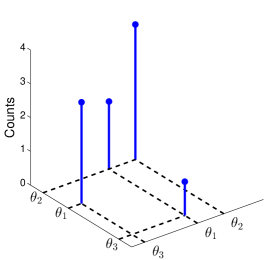
(a)	(b)	(c)

Figure 2: An example of (a) the restriction on $[0,1]^{2}$ of an atomic measure $D$, (b) the corresponding directed multigraph, and (c) corresponding undirected graph.

Our generative approach for modeling $D$ associates with each node $\theta_{i}$ a sociability parameter $w_{i}>0$ defined via the atomic random measure

$$W=\sum_{i=1}^{\infty}w_{i}\delta_{\theta_{i}},$$ (16)

which we take to be distributed according to a homogeneous CRM, $W\sim\mbox{CRM}(\rho,\lambda)$. Given $W$, $D$ is simply generated from a Poisson process (PP) with intensity given by the product measure $\widetilde{W}=W\times W$ on $\mathbb{R}_{+}^{2}$:

$$D\mid W\sim\mbox{PP}(W\times W).$$ (17)

That is, informally, the individual counts $n_{ij}$ are generated as $\mbox{Poisson}(w_{i}w_{j})$. By construction, for any $A,B\subset\mathbb{R}$, we have $\widetilde{W}(A\times B)=W(A)W(B)$. On any bounded interval $A$ of $\mathbb{R}_{+}$, $W(A)<\infty$ implying $\widetilde{W}(A\times A)$ has finite mass.

3.2 Undirected graphs

We now turn to the primary focus of modeling undirected graphs. Similarly to the directed case of Section 3.1, we represent an undirected graph using an atomic measure

$$Z=\sum_{i=1}^{\infty}\sum_{j=1}^{\infty}z_{ij}\delta_{(\theta_{i},\theta_{j})},$$

with the convention $z_{ij}=z_{ji}\in\{0,1\}$. Here, $z_{ij}=z_{ji}=1$ indicates an undirected edge between nodes $\theta_{i}$ and $\theta_{j}$. We arise at the undirected graph via a simple transformation of the directed graph: set $z_{ij}=z_{ji}=1$ if $n_{ij}+n_{ji}>0$ and $z_{ij}=z_{ji}=0$ otherwise. That is, place an undirected edge between nodes $\theta_{i}$ and $\theta_{j}$ if and only if there is at least one directed interaction between the nodes. Note that in this definition of an undirected graph, we allow self-edges. This could represent, for example, a person posting a message on his or her own profile page. The resulting hierarchical model is as follows:

$$\begin{aligned} \begin{array}[]{ll}W=\sum_{i=1}^{\infty}w_{i}\delta_{\theta_{i}}&W\sim\mbox{CRM}(\rho,\lambda)\\ D=\sum_{i=1}^{\infty}\sum_{j=1}^{\infty}n_{ij}\delta_{(\theta_{i},\theta_{j})}&D\mid W\sim\text{PP}\left(W\times W\right)\\ Z=\sum_{i=1}^{\infty}\sum_{j=1}^{\infty}\min(n_{ij}+n_{ji},1)\delta_{(\theta_{i},\theta_{j})}.&\end{array}\end{aligned}$$ (18)

This process is depicted graphically in Figure 3.

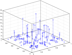
(a) $\widetilde{W}=W\times W$

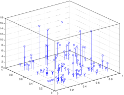
(b) Integer point process $D$

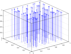
(c) Point process $Z$

Figure 3: An example of (a) the product measure $\widetilde{W}=W\times W$ for CRM $W$, (b) a draw of the directed multigraph measure $D\mid W\sim PP(W\times W)$, (c) corresponding undirected measure $Z=\sum_{i=1}^{\infty}\sum_{j=1}^{\infty}\min(n_{ij}+n_{ji},1)\delta_{(\theta_{i},\theta_{j})}$.

Equivalently, given the sociability parameters $w=\{w_{i}\}$, we can directly specify the undirected graph model as

$$\Pr(z_{ij}=1\mid w)=\left\{\begin{array}[c]{ll}1-\exp(-2w_{i}w_{j})&i\neq j\\ 1-\exp(-w_{i}^{2})&i=j.\end{array}\right.$$ (21)

To see the equivalence between this formulation and the one obtained from manipulating the directed multigraph, note that for $i\neq j$, $\Pr(z_{ij}=1\mid w)=\Pr(n_{ij}+n_{ji}>0\mid w)$. By properties of the Poisson process, $n_{ij}$ and $n_{ji}$ are independent random variables conditioned on $W$. The sum of two Poisson random variables, each with rate $w_{i}w_{j}$, is again Poisson with rate $2w_{i}w_{j}$. The result (21) arises from the fact that $\Pr(n_{ij}+n_{ji}>0\mid w)=1-\Pr(n_{ij}+n_{ji}=0\mid w)$. Likewise, the $i=j$ case arises using a similar reasoning for $\Pr(z_{ii}=1\mid w)=\Pr(n_{ii}>0\mid w)$.

Graph restrictions

Our general network process is defined on $\mathbb{R}_{+}^{2}$ and, due to the fact that $W(\mathbb{R}_{+})=\infty$, yields an infinite number of edges. In applications, we are typically interested in considering graphs with a finite number of edges, but without a bound on or prespecification of this finite number. We therefore consider restrictions $D_{\alpha}$ and $Z_{\alpha}$ of $D$ and $Z$, respectively, to the box $[0,\alpha]^{2}$ and in Section 6 examine methods for inferring $\alpha$. We also denote by $W_{\alpha}$ and $\lambda_{\alpha}$ the corresponding CRM and Lebesgue measure on $[0,\alpha]$. We write $Z_{\alpha}^{\ast}=Z_{\alpha}([0,\alpha]^{2})$, the total mass on $[0,\alpha]^{2}$, and similarly for $D_{\alpha}^{\ast}$ and $W_{\alpha}^{\ast}$. By definition, $D_{\alpha}$ is drawn from a Poisson process with finite mean measure $W_{\alpha}\times W_{\alpha}$, so we have the following generative model for directly simulating $D_{\alpha}$ and $Z_{\alpha}$:

$$W_{\alpha} \sim\mbox{CRM}(\rho,\lambda_{\alpha})$$

$$D_{\alpha}^{\ast}|W^{\ast}_{\alpha} \sim\mbox{Poisson}(W_{\alpha}^{\ast\ 2}).$$

For $$k=1,\ldots,D_{\alpha}^{\ast} j=1,2$$ and

$$U_{kj}|W_{\alpha} \overset{iid}{\sim}\frac{W_{\alpha}}{W_{\alpha}^{\ast}}$$

$$D_{\alpha} =\sum_{k=1}^{D_{\alpha}^{\ast}}\delta_{(U_{k1},U_{k2})}.$$ (22)

Here, the variables $U_{kj}\in\mathbb{R}_{+}$ correspond to nodes in the graph, and pairs of variables $(U_{k1},U_{k2})$ correspond to a directed edge from node $U_{k1}$ to node $U_{k2}$. The number of directed edges, $D_{\alpha}^{\ast}$, depends on the total mass of the CRM, $W_{\alpha}^{\ast}$. For each such directed edge, the defining nodes $U_{kj}$ are drawn from a normalized CRM, $\frac{W_{\alpha}}{W_{\alpha}^{\ast}}$; since $\frac{W_{\alpha}}{W_{\alpha}^{\ast}}$ is discrete with probability 1, the $U_{kj}$ take a number $N_{\alpha}\leq 2D_{\alpha}^{\ast}$ of distinct values. That is, $N_{\alpha}$ corresponds to the number of nodes with degree at least one in the network. Recall that the undirected network construction simply forms an undirected edge between a set of nodes if there exists at least one directed edge between them. If we consider unordered pairs $\{U_{k1},U_{k2}\}$, the number of such unique pairs takes a number $N_{\alpha}^{(e)}\leq D_{\alpha}^{\ast}$ of distinct values, where $N_{\alpha}^{(e)}$ corresponds to the number of edges in the undirected network.

The construction (22), enables us to re-express our Cox process model in terms of normalized CRMs (Regazzini, Lijoi and Prünster, 2003). This is very attractive both practically and theoretically; as we show in Section 5, one can use this framework to build on the various results on urn processes and power-law properties of normalized CRMs in order to get exact samplers for our graph models as well as to show its sparsity.

Finite-dimensional generative process

We now describe the urn formulation that allows us to obtain a finite-dimensional generative process. Recall that in practice, we cannot sample $W_{\alpha}\sim\mbox{CRM}(\rho,\lambda_{\alpha})$ if the CRM is infinite activity.

Let $(U^{\prime}_{1},\ldots,U^{\prime}_{2D_{\alpha}^{\ast}})=(U_{11},U_{12},\ldots U_{D_{\alpha}^{\ast}1},U_{D_{\alpha}^{\ast}2})$. For some classes of Lévy measure $\rho$, it is possible to integrate out the normalized CRM $\mu_{\alpha}=\frac{W_{\alpha}}{W_{\alpha}^{\ast}}$ in (22) and derive the conditional distribution of $U^{\prime}_{n+1}$ given $(W_{\alpha}^{\ast},U^{\prime}_{1},\ldots,U^{\prime}_{n})$. We first recall some background on random partitions. As $\mu_{\alpha}$ is discrete with probability 1, variables $U^{\prime}_{1},\ldots,U^{\prime}_{n}$ take $k\leq n$ distinct values $\widetilde{U}^{\prime}_{j}$, with multiplicities $1\leq m_{j}\leq n$. The distribution on the underlying partition is usually defined in terms of an exchangeable partition probability function (EPPF) (Pitman, 1995) $\Pi_{n}^{(k)}(m_{1},\ldots,m_{k}|W_{\alpha}^{\ast})$ which is symmetric in its arguments. The predictive distribution of $U^{\prime}_{n+1}$ given $(W_{\alpha}^{\ast},U^{\prime}_{1},\ldots,U^{\prime}_{n})$ is then given in terms of the EPPF:

$$U^{\prime}_{n+1}|(W_{\alpha}^{\ast},U^{\prime}_{1},\ldots,U^{\prime}_{n}) \sim\frac{\Pi_{n+1}^{(k+1)}(m_{1},\ldots,m_{k},1|W_{\alpha}^{\ast})}{\Pi_{n}^{(k)}(m_{1},\ldots,m_{k}|W_{\alpha}^{\ast})}\frac{1}{\alpha}\lambda_{\alpha}$$

$$+\sum_{j=1}^{k}\frac{\Pi_{n+1}^{(k)}(m_{1},\ldots,m_{j}+1,\ldots,m_{k}|W_{\alpha}^{\ast})}{\Pi_{n}^{(k)}(m_{1},\ldots,m_{k}|W_{\alpha}^{\ast})}\delta_{\widetilde{U}^{\prime}_{j}}.$$ (23)

Using this urn representation, we can rewrite our generative process as

$$W_{\alpha}^{\ast} \sim P_{W_{\alpha}^{\ast}}$$

$$D_{\alpha}^{\ast}|W^{\ast}_{\alpha} \sim\mbox{Poisson}(W_{\alpha}^{\ast\ 2}).$$

$$(U_{kj})_{k=1,\ldots,D_{\alpha}^{\ast};j=1,2}|W_{\alpha}^{\ast} \sim\text{Urn process \eqref{eq:generalurn}}$$

$$D_{\alpha} =\sum_{k=1}^{D_{\alpha}^{\ast}}\delta_{(U_{k1},U_{k2})},$$ (24)

where $P_{W_{\alpha}^{\ast}}$ is the distribution of the CRM total mass, $W_{\alpha}^{\ast}$. The representation of (24) can be used to sample exactly from our graph model, assuming we can sample from $P_{W_{\alpha}^{\ast}}$ and evaluate the EPPF. In Section 5 we show that this is indeed possible for specific CRMs of interest. If this is not possible, in Section 4.4 we present alternative, though potentially more computationally complex, methods for simulation.

3.3 Bipartite graphs

The above construction can also be extended to bipartite graphs. Let $V=(\theta_{1},\theta_{2},...)$ and $V^{\prime}=(\theta^{\prime}_{1},\theta^{\prime}_{2},...)$ be two countably infinite set of nodes with $\theta_{i},\theta^{\prime}_{i}\in\mathbb{R}_{+}$. We assume that only connections between nodes of different sets are allowed.

We represent the directed bipartite multigraph of interest using an atomic measure on $\mathbb{R}_{+}^{2}$

$$D=\sum_{i=1}^{\infty}\sum_{j=1}^{\infty}n_{ij}\delta_{(\theta_{i},\theta^{\prime}_{j})},$$ (25)

where $n_{ij}$ counts the number of directed edges from node $\theta_{i}$ to node $\theta^{\prime}_{j}$. Similarly, the bipartite graph is represented by an atomic measure

$$Z=\sum_{i=1}^{\infty}\sum_{j=1}^{\infty}z_{ij}\delta_{(\theta_{i},\theta^{\prime}_{j})}.$$

Our bipartite graph formulation introduces two CRMs, $W\sim\mbox{CRM}(\rho,\lambda)$ and $W^{\prime}\sim\mbox{CRM}(\rho^{\prime},\lambda)$, whose jumps correspond to sociability parameters for nodes in sets $V$ and $V^{\prime}$, respectively. The generative model for the bipartite graph mimics that of the non-bipartite one:

$$\begin{aligned} \begin{array}[]{ll}W=\sum_{i=1}^{\infty}w_{i}\delta_{\theta_{i}}&W\sim\mbox{CRM}(\rho,\lambda)\\ W^{\prime}=\sum_{j=1}^{\infty}w^{\prime}_{j}\delta_{\theta^{\prime}_{j}}&W^{\prime}\sim\mbox{CRM}(\rho^{\prime},\lambda)\\ D=\sum_{i=1}^{\infty}\sum_{j=1}^{\infty}n_{ij}\delta_{(\theta_{i},\theta^{\prime}_{j})}&D\mid W,W^{\prime}\sim\text{PP}\left(W\times W^{\prime}\right)\\ Z=\sum_{i=1}^{\infty}\sum_{j=1}^{\infty}\min(n_{ij},1)\delta_{(\theta_{i},\theta^{\prime}_{j})}.&\end{array}\end{aligned}$$ (26)

The model (26) has been proposed by Caron (2012) in a slightly different formulation. Here, we recast this model within our general framework making connections with an urn representation and the Kallenberg theory of exchangeability, both of which enable new theoretical and practical insights.

4 General properties and simulation

We provide here general properties of our network model depending on the properties of the Lévy intensity $\rho.$ In the next section, we provide more refined properties, depending on specific choices of $\rho$.

4.1 Exchangeability under the Kallenberg framework

Proposition 3

(Joint exchangeability of the undirected graph measure).
 For any CRM $W\sim\operatorname{CRM}(\rho,\lambda)$, the point process $Z$ defined by (18), or equivalently by (21), is jointly exchangeable.

Proof 4.4.

The proof follows from the properties of $W\sim\operatorname{CRM}(\rho,\lambda)$. Let $A_{i}=[h(i-1),hi]$ for $h>0$ and $i\in\mathbb{N}.$ We have

$$(W(A_{i}))\overset{d}{=}(W(A_{\pi(i)}))$$ (27)

for any permutation $\pi$ of $\mathbb{N}$. As $D(A_{i}\times A_{j})\sim\mbox{Poisson}(W(A_{i})W(A_{j}))$, it follows that

$$(D(A_{i}\times A_{j}))\overset{d}{=}(D(A_{\pi(i)}\times A_{\pi(j)}))$$ (28)

for any permutation $\pi$ of $\mathbb{N}$. Joint exchangeability of $Z$ follows directly.

We now reformulate our network process in the Kallenberg representation of (7). Due to exchangeability, we know that such a representation exits. What we show here is that our CRM-based formulation has an analytic and interpretable representation. In particular, the CRM $W$ can be constructed from a two-dimensional unit-rate Poisson process on $\mathbb{R}_{+}^{2}$ using the inverse Lévy method (Khintchine, 1937; Ferguson and Klass, 1972). Let $(\theta_{i},\vartheta_{i})$ be a unit-rate Poisson process on $\mathbb{R}_{+}^{2}$. Let $\overline{\rho}(x)$ be the tail Lévy intensity defined in (14). Then the CRM $W=\sum w_{i}\delta_{\theta_{i}}$ with Lévy measure $\rho(dw)d\theta$ can be constructed from the bi-dimensional point process by taking $w_{i}=\overline{\rho}^{-1}(\vartheta_{i})$. $\overline{\rho}^{-1}$ is a monotone function, known as the inverse Lévy intensity. It follows that our undirected graph model can be formulated under the representation of (7) by selecting any $\alpha_{0}$, $\beta_{0}=\gamma_{0}=0$, $g=g^{\prime}=0$, $h=h^{\prime}=l=l^{\prime}=0$ and

$$f(\alpha_{0},\vartheta_{i},\vartheta_{j},\zeta_{\{i,j\}})=\left\{\begin{array}[c]{ll}1&\zeta_{\{i,j\}}\leq M(\vartheta_{i},\vartheta_{j})\\ 0&\text{otherwise}\end{array}\right.$$ (31)

where $M:\mathbb{R}_{+}^{2}\rightarrow[0,1]$ is defined by

$$M(\vartheta_{i},\vartheta_{j})=\left\{\begin{array}[c]{ll}1-\exp(-2\overline{\rho}^{-1}(\vartheta_{i})\overline{\rho}^{-1}(\vartheta_{j}))&\text{if }\vartheta_{i}\neq\vartheta_{j}\\ 1-\exp(-\overline{\rho}^{-1}(\vartheta_{i})^{2})&\text{if }\vartheta_{i}=\vartheta_{j}.\end{array}\right.$$

In Section 5, we provide explicit forms for $\overline{\rho}$ depending on our choice of Lévy intensity $\rho$. The expression (31) represents a direct analog to that of (6) arising from the Aldous-Hoover framework. In particular, $M$ here is akin to the graphon $\omega$, and thus allows us to connect our CRM-based formulation with the extensive literature on graphons. An illustration of the network construction from the Kallenberg representation, including the function $M$, is provided in Figure 4. Note that had we started from the Kallenberg representation and selected an $f$ (or $M$) arbitrarily, we would likely not have yielded a network model with the normalized CRM interpretation that enables both interpretability and analysis of network properties, such as those presented in Section 5.3.

Figure 4: Illustration of the model construction based on the Kallenberg representation. (left) A unit-rate Poisson process $(\theta_{i},\vartheta_{i})$, $i\in\mathbb{N}$ on $[0,\alpha]\times\mathbb{R}_{+}$. (right) For each pair $\{i,j\}\in\widetilde{\mathbb{N}}^{2}$, set $z_{ij}=z_{ji}=1$ with probability $M(\vartheta_{i},\vartheta_{j})$. Here, $M$ is indicated by the blue shading (darker shading indicates higher value) for a stable process (generalized gamma process with $\tau=0$). In this case there is an analytic expression for $\overline{\rho}^{-1}$ and therefore $M$.

For the bipartite graph, an application of Kallenberg’s representation theorem for separate exchangeability can likewise be made.

4.2 Sparsity

In this section we state the sparsity properties of our graph model, which relate to the properties of the Lévy intensity $\rho$. Of particular interest is the notion of a regularly varying Lévy intensity (Karlin, 1967; Gnedin, Pitman and Yor, 2006; Gnedin, Hansen and Pitman, 2007), defined as follows.

Definition 4.5.

(Regular variation) Let $W\sim\operatorname{CRM}(\rho,\lambda)$. The CRM is said to be regularly varying if the tail Lévy intensity verifies

$$\overline{\rho}(x)\overset{x\downarrow 0}{\sim}\ell(1/x)x^{-\sigma}$$ (32)

for $\sigma\in(0,1)$ where $\ell$ is a slowly varying function satisfying $\lim_{t\rightarrow\infty}\ell(at)/\ell(t)=1$ for any $a>0$. For example, constant and logarithmic functions are slowly varying. The equivalence notation $f(x)\overset{x\downarrow 0}{\sim}g(x)$ is used for $\lim_{x\rightarrow 0}\frac{f(x)}{g(x)}=1$ (not to be confused with the notation $\sim$ alone for ‘distributed from’).

As a trivial (and degenerate) example of obtaining sparse graphs, we note that if $\rho(dw)=0$, then $W([0,\infty))=0$ almost surely and there are no edges, $N_{\alpha}^{(e)}=0$, and thus no nodes of degree at least one, $N_{\alpha}=0$, for all values of $\alpha$. We consider more general Lévy intensities in Theorem 4.6. In this theorem, we follow the notation of Janson (2011) for probability asymptotics (see Appendix A.1 for details).

Theorem 4.6.

Consider the point process $Z$ with $\rho(w)\neq 0$. Let $\psi(t)$, defined in (13), be the Laplace exponent and $\psi^{\prime}(t)$ its first derivative; here, $\lim_{t\rightarrow 0}\psi^{\prime}(t)=\mathbb{E}[W_{1}^{\ast}]$, the expected total mass for $\alpha=1$. Let $N_{\alpha}^{(e)}$ be the number of edges in the undirected graph restriction $Z_{\alpha}$, and $N_{\alpha}$ be the number of nodes.
If the CRM $W$ is finite-activity (i.e., is obtained from a compound Poisson process):

$$\int_{0}^{\infty}\rho(w)dw<\infty,$$

then the number of edges scales quadratically with the number of nodes

$$N_{\alpha}^{(e)}=\Theta(N_{\alpha}^{2})$$ (33)

almost surely as $\alpha$ tends to infinity, and the graph is dense.
If the CRM is infinite-activity, i.e.

$$\int_{0}^{\infty}\rho(w)dw=\infty$$

and

$$\lim_{t\rightarrow 0}\psi^{\prime}(t)<\infty,$$ (34)

then the number of edges scales sub-quadratically with the number of nodes

$$N_{\alpha}^{(e)}=o(N_{\alpha}^{2})$$ (35)

almost surely as $\alpha$ tends to infinity, and the graph is sparse.

The sparsity regime is linked to the property of regular variation of the Lévy intensity (Definition 4.5). If the Lévy intensity $\rho$ is regularly varying, i.e. if there exists a slowly varying function $\ell$ such that $\overline{\rho}(x)\overset{x\downarrow 0}{\sim}\ell(1/x)x^{-\sigma}$ with $\sigma\in(0,1)$, and if additionally $\lim_{t\rightarrow\infty}\ell(t)>0$, then

$$N_{\alpha}^{(e)}=O\left(N_{\alpha}^{\frac{2}{1+\sigma}}\right)$$ (36)

almost surely.

Theorem 4.6 is a direct consequence of two theorems that we state now and prove in Appendix A. The first theorem states that the number of edges grows quadratically with $\alpha$, while the second states that the number of nodes scales superlinearly with $\alpha$ for infinite-activity CRMs, and linearly otherwise.

Theorem 4.7.

Consider the point process $Z$ with $\rho(w)\neq 0$. If $\lim_{t\rightarrow 0}\psi^{\prime}(t)=\mathbb{E}[W_{1}^{\ast}]<\infty$, then the number of edges in $Z_{\alpha}$ grows quadratically with $\alpha$:

$$N_{\alpha}^{(e)}=\Theta(\alpha^{2})$$ (37)

almost surely. Otherwise, $N_{\alpha}^{(e)}=\Omega(\alpha^{2})$.

Theorem 4.8.

Consider the point process $Z$ with $\rho(w)\neq 0$. Then

$$N_{\alpha}=\left\{\begin{array}[c]{ll}\Theta(\alpha)&\text{if }W\text{ is a finite-activity CRM}\\ \omega(\alpha)&\text{if }W\text{ is an infinite-activity CRM}\end{array}\right.$$ (38)

almost surely as $\alpha\rightarrow\infty$. In words, the number of nodes in $Z_{\alpha}$ scales linearly with $\alpha$ for finite-activity CRMs and superlinearly with $\alpha$ for infinite-activity CRMs. In particular, for a regularly varying Lévy intensity with $\lim_{t\rightarrow\infty}\ell(t)>0$, we have

$$N_{\alpha}=\Omega(\alpha^{\sigma+1})$$ (39)

almost surely as $\alpha\rightarrow\infty$.

4.3 Interactions between groups

For any disjoint set of nodes $A,B\subset\mathbb{R}_{+}$, $A\cap B=\emptyset$, the probability that there is at least one connection between a node in $A$ and a node in $B$ is given by

$$\Pr(Z(A\times B)>0|W)=1-\exp(-2W(A)W(B)).$$

That is, the probability of a between-group edge depends on the sum of the sociabilities in each group, $W(A)$ and $W(B)$, respectively.

4.4 Simulation

To simulate an undirected graph, we harness the directed multigraph representation. That is, we first sample a directed multigraph and then transform it to an undirected graph as described in Section 3.2. One might imagine simulating a directed network by first sampling $W_{\alpha}$ and then sampling $D_{\alpha}$ given $W_{\alpha}$. However, recall that $W_{\alpha}$ may have an infinite number of jumps. One approximate approach to coping with this issue, which is possible for some Lévy intensities $\rho$, is to resort to adaptive thinning (Lewis and Shedler, 1979; Ogata, 1981; Favaro and Teh, 2013). A related alternative approximate approach, but applicable to any Lévy intensity $\rho$ satisfying (12), is the inverse Lévy method. This method first defines a threshold $\varepsilon$ and then samples the weights $\Omega=\{w_{i}|w_{i}>\varepsilon\}$ using a Poisson measure on $[\varepsilon,+\infty]$. One then simulates $D_{\alpha}$ using these truncated weights $\Omega$.

A naive application of this truncated method that considers sampling directed or undirected edges as in (18) or (21), respectively, can prove computationally problematic since a large number of possible edges must be considered (one Poisson/Bernoulli draw for each $(\theta_{i},\theta_{j})$ pair for the directed/undirected case). Instead, we can harness the Cox process representation and resulting sampling procedure of (22) to first sample the total number of directed edges and then their specific instantiations. More specifically, to approximately simulate a point process on $[0,\alpha]^{2}$, we use the inverse Lévy method to sample

$$\Pi_{\alpha,\varepsilon}=\{(w,\theta)\in\Pi,0<\theta\leq\alpha,w>\varepsilon\}.$$ (40)

Let $W_{\alpha,\varepsilon}=\sum_{i=1}^{K}w_{i}\delta_{\theta_{i}}$ be the associated truncated CRM and $W_{\alpha,\varepsilon}^{\ast}=W_{\alpha,\varepsilon}([0,\alpha])$ its total mass. We then sample $D_{\alpha,\varepsilon}^{\ast}$ and $U_{k,j}$ as in (22) and set $D_{\alpha,\varepsilon}=\sum_{k=1}^{D_{\alpha,\varepsilon}^{\ast}}\delta_{(U_{k1},U_{k2})}$. The undirected graph measure $Z_{\alpha,\varepsilon}$ is set to the manipulation of $D_{\alpha,\varepsilon}$ as in (18).

In the next section, we show that it is possible to sample a graph exactly via an urn scheme when considering the special case of generalized gamma processes, which includes the standard gamma process.

5 Special cases

In this section, we examine the properties of various models and their link to classical random graph models depending on the Lévy measure $\rho$. We show that in generalized gamma process case, the resulting graph can be either dense or sparse, with the sparsity tuned by a single hyperparameter. We focus on the undirected graph case, but similar results can be obtained for directed multigraphs and bipartite graphs.

5.1 Poisson process

Consider a Poisson process with fixed increments $a$ and

$$\rho(dw)=\delta_{w_{0}}(dw),$$

where $\delta_{w_{0}}$ is the dirac delta mass at $w_{0}>0$. Recalling the definition $\overline{\rho}(x)=\int_{x}^{\infty}\rho(dw)$, in this case, we have

$$\overline{\rho}(x)=\left\{\begin{array}[c]{ll}1&\text{if }x<w_{0}\\ 0&\text{otherwise}.\end{array}\right.$$

Ignoring self-edges, the graph construction can be described as follows. To sample $W_{\alpha}\sim\mbox{PP}(\rho,\lambda_{\alpha})$, we generate $n\sim\mbox{Poisson}(\alpha)$ and then sample $\theta_{i}\sim\mbox{Uniform}([0,\alpha])$ for $i=1,\ldots n$. We then sample edges according to (21): For $0<i<j<n$, set $z_{ij}=z_{ji}=1$ with probability $1-$exp$(-2w_{0}^{2})$ and 0 otherwise. The model is therefore equivalent to the Erdös-Rényi random graph model $G(n,p)$ with $n\sim\mbox{Poisson}(\alpha)$ and $p=1-\exp(-2w_{0}^{2})$. Therefore, this choice of $\rho$ leads to a dense graph where the number of edges grows quadratically with the number of nodes $n$.

5.2 Compound Poisson process

A compound Poisson process is one where

$$\rho(dw)=h(w)dw$$

and $h:\mathbb{R}_{+}\rightarrow\mathbb{R}_{+}$ is such that $\int_{0}^{\infty}h(w)dw=1.$ In this case, we have

$$\overline{\rho}(x)=1-H(x)$$

where $H$ is the distribution function associated with $h$. Here, we arrive at a framework similar to the standard graphon. Leveraging the Kallenberg representation of (31), we first sample $n\sim\mbox{Poisson}(\alpha)$. Then, for $i=1,\ldots n$ we set $z_{ij}=z_{ji}=1$ with probability $M(U_{i},U_{j})$ where $U_{i}$ are uniform variables and $M$ is defined by

$$M(U_{i},U_{j})=1-\exp(-2H^{-1}(U_{i})H^{-1}(U_{j})).$$

This representation is the same as with the Aldous-Hoover theorem, where the number of nodes is random and follows a Poisson distribution. As such, the resulting random graph is either trivially empty or dense.

5.3 Generalized gamma process

The generalized gamma process (Hougaard, 1986; Aalen, 1992; Lee and Whitmore, 1993; Brix, 1999) (GGP) is a flexible two-parameter CRM, with interpretable parameters and remarkable conjugacy properties (Lijoi, Mena and Prünster, 2007; Caron, Teh and Murphy, 2014). The process is known as the Hougaard process (Hougaard, 1986) when $\lambda$ is the Lebesgue measure, as in this paper, but we will use the term GGP in the rest of this paper. The Lévy intensity of the GGP is given by

$$\rho(dw)=\frac{1}{\Gamma(1-\sigma)}w^{-1-\sigma}\exp(-\tau w)dw,$$ (41)

where the two parameters $(\sigma,\tau)$ verify

$$(\sigma,\tau)\in(-\infty,0]\times(0,+\infty)\text{ or }(\sigma,\tau)\in(0,1)\times[0,+\infty).$$ (42)

The GGP has different properties if $\sigma\geq 0$ or $\sigma<0$. When $\sigma<0$, the GGP is a finite-activity CRM; more precisely, the number of jumps in $[0,\alpha]$ is finite w.p. 1 and drawn from a Poisson distribution with rate $-\frac{\alpha}{\sigma}\tau^{\sigma}$ while the jumps $w_{i}$ are i.i.d. $\operatorname*{Gamma}(-\sigma,\tau)$.

When $\sigma\geq 0$, the GGP has an infinite number of jumps over any interval $[s,t]$. It includes as special cases the gamma process ($\sigma=0$, $\tau>0$), the stable process ($\sigma\in(0,1)$, $\tau=0$) and the inverse-Gaussian process ($\sigma=\frac{1}{2}$,$\tau>0$).

The tail Lévy intensity of the GGP is given by

$$\overline{\rho}(x)=\int_{x}^{\infty}\frac{1}{\Gamma(1-\sigma)}w^{-1-\sigma}\exp(-\tau w)dw=\left\{\begin{array}[c]{cc}\frac{\tau^{\sigma}\Gamma(-\sigma,\tau x)}{\Gamma(1-\sigma)}&\text{if }\tau>0\\ \frac{x^{-\sigma}}{\Gamma(1-\sigma)\sigma}&\text{if }\tau=0,\end{array}\right.$$

where $\Gamma(a,x)$ is the incomplete gamma function. Example realizations of the process for various values of $\sigma\geq 0$ are displayed in Figure 5 alongside a realization of an Erdös-Rényi graph.

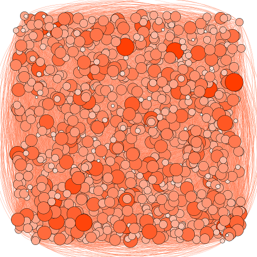
(a) $G(1000,0.05)$

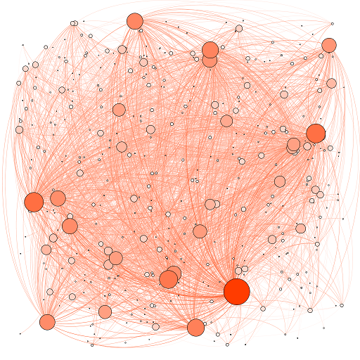
(b) $GGP(100,2,0)$

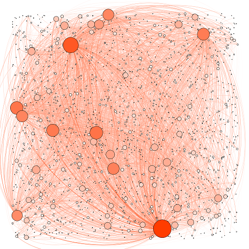
(c) $GGP(100,2,0.5)$

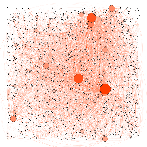
(d) $GGP(100,2,0.8)$

Figure 5: Sample graphs: (a) Erdös-Rényi graph $G(n,p)$ with $n=1000$ and $p=0.05$ (b-c) Generalized gamma process graph $GGP(\alpha,\tau,\sigma)$ with $\alpha=100$, $\tau=2$ and (b) $\sigma=0$, (c) $\sigma=0.5$, (d) $\sigma=0.8$. The size of a node is proportional to its degree. Graphs have been generated with the software Gephi.

Exact sampling via an urn approach

In the case $\sigma\geq 0$, $W_{\alpha}^{\ast}$ is an exponentially tilted stable random variable, for which exact samplers exist (Devroye, 2009). As shown by Pitman (2003) (see also (Lijoi, Prünster and Walker, 2008)), the EPPF conditional on the total mass $W_{\alpha}^{\ast}=t$ only depends on the parameter $\sigma$ (and not $\tau,\alpha$) and is given by

$$\Pi_{k}^{(n)}(m_{1},\ldots,m_{k}|t)=\frac{\sigma^{k}t^{-n}}{\Gamma(n-k\sigma)g_{\sigma}(t)}\int_{0}^{t}s^{n-k\sigma-1}g_{\sigma}(t-s)ds\left(\prod_{i=1}^{k}\frac{\Gamma(m_{i}-\sigma)}{\Gamma(1-\sigma)}\right),$$ (43)

where $g_{\sigma}$ is the pdf of the positive stable distribution. Plugging the EPPF of (43) in to (23) yields the urn process for sampling in the GGP case. In particular, one can use the generative process (24) in order to sample exactly from the model.

In the special case of the gamma process ($\sigma=0$), $W_{\alpha}^{\ast}$ is a Gamma$(\alpha,\tau)$ random variable and the resulting urn process is given by (Blackwell and MacQueen, 1973; Pitman, 1996):

$$U^{\prime}_{n+1}|(W_{\alpha}^{\ast},U^{\prime}_{1},\ldots,U^{\prime}_{n}) \sim\frac{1}{\alpha+n}\lambda_{\alpha}+\sum_{j=1}^{k}\frac{m_{j}}{\alpha+n}\delta_{\widetilde{U}^{\prime}_{j}}.$$ (44)

When $\sigma<0$, the GGP is a compound Poisson process and can thus be sampled exactly.

Expected number of nodes and edges

In Theorem 5.9, we consider bounds on the expected number of nodes in the gamma process case ($\sigma=0,\tau>0$), and the expected number of edges in the multigraph. The proof is in Appendix C.

Theorem 5.9.

For any $\varepsilon\in(0,1)$,

$$\alpha\log\left(1+\varepsilon\frac{2(\alpha+1)}{\tau^{2}}\right)\left(1-\frac{c_{1}(\alpha)}{1-\varepsilon^{2}}\right)\leq\mathbb{E}[N_{\alpha}]\\ \leq\alpha\log\left(1+\frac{2(\alpha+1)}{\tau^{2}}\right)+\frac{2(\alpha+1)}{\tau^{2}+2(\alpha+1)},$$ (45)

where $c_{1}(\alpha)=\frac{Var(D_{\alpha}^{\ast})}{\mathbb{E}[D_{\alpha}^{\ast}]^{2}}=\frac{\tau^{2}}{\alpha(\alpha+1)}\left(1+\frac{4\alpha+6}{\tau^{2}}\right)$ is a decreasing function of $\alpha$ with $c(\alpha)\rightarrow 0$ as $\alpha\rightarrow\infty.$ Consequently,

$$\mathbb{E}[N_{\alpha}]=\Theta(\alpha\log\alpha).$$ (46)

Let $D_{\alpha}^{\ast}$ be the number of edges in the directed multigraph. Then

$$\mathbb{E}[D_{\alpha}^{\ast}]=\frac{\alpha(\alpha+1)}{\tau^{2}}\quad Var[D_{\alpha}^{\ast}]=\frac{\alpha(\alpha+1)}{\tau^{2}}\left(1+\frac{4\alpha+6}{\tau^{2}}\right).$$

Power-law properties

In Theorem 5.10, we show that the GGP directed multigraph has a power-law degree distribution. A corresponding theorem in the undirected graph case is challenging to show and beyond the scope of this paper, but our empirical results of Figure 6 demonstrate that such a power-law property likely holds for the undirected case as well.

Theorem 5.10.

Let $N_{\alpha,j}$, $j\geq 1$ be the number of nodes in the directed multigraph $D_{\alpha}$ with $j$ outgoing or incoming edges (a self edge counts twice for a given node). Then we have the following asymptotic results for the GGP:

$$\frac{N_{\alpha,j}}{N_{\alpha}}\,\overset{\alpha\uparrow\infty}{\longrightarrow}\,\,\,p_{\sigma,j}=\frac{\sigma\Gamma(j-\sigma)}{\Gamma(1-\sigma)\Gamma(j+1)},$$ (47)

almost surely, for fixed $j$. In particular, for large $j$, we have tail behavior

$$p_{\sigma,j}\overset{j\uparrow\infty}{\sim}\frac{\sigma}{\Gamma(1-\sigma)}j^{-1-\sigma}$$ (48)

corresponding to a power-law behavior.

The proof, which builds on the asymptotic properties of the normalized GGP (Lijoi, Mena and Prünster, 2007), is given in Appendix C.

Sparsity

The following theorem states that the GGP parameter $\sigma$ tunes the sparsity of the graph. When $\sigma<0$, the graph is dense, whereas it is sparse when $\sigma\geq 0$.

Theorem 5.11.

Let $N_{\alpha}$ be the number of nodes and $N_{\alpha}^{(e)}$ the number of edges in the undirected graph restriction, $Z_{\alpha}$. Then

$$N_{\alpha}^{(e)}=\left\{\begin{tabular}[]{ll}$\Theta\left(N_{\alpha}^{2}\right)$&if $\sigma<0$\\ $o\left(N_{\alpha}^{2}\right)$&if $\sigma\in[0,1),\tau>0$\\ $O\left(N_{\alpha}^{2/(1+\sigma)}\right)$&if $\sigma\in(0,1),\tau>0$\end{tabular}\right.$$

almost surely as $\alpha\rightarrow\infty$. That is, the underlying graph is sparse if $\sigma\geq 0$ and dense otherwise.

Proof 5.12.

For $\sigma<0$, the CRM is finite-activity and thus Theorem 4.6 implies that the graph is dense. When $\sigma\geq 0$ the CRM is infinite-activity; moreover, for $\tau>0$, $\mathbb{E}[W^{*}_{\alpha}]<\infty$, and thus Theorem 4.6 implies that the graph is sparse. More precisely, for $\sigma>0$, the tail Lévy intensity has the asymptotic behavior

$$\overline{\rho}(x)\overset{x\downarrow 0}{\sim}\frac{\alpha}{\sigma\Gamma(1-\sigma)}x^{-\sigma}$$

and so Theorem 5.11 follows directly from Theorem 4.6.

Remark 5.13.

The proof technique requires a finite first moment for the total mass $W^{*}_{\alpha}$, and thus excludes the stable process $(\tau=0,\sigma\in(0,1))$, although we conjecture that the graph is also sparse in that case.

Empirical analysis of graph properties

For the GGP-based formulation, we provide an empirical analysis of our network properties in Figure 6 by simulating undirected graphs using the approach described in Section 4.4 for various values of $\sigma,\tau$. We compare to an Erdös Rényi random graph, preferential attachment (Barabási and Albert, 1999), and the Bayesian nonparametric network model of (Lloyd et al., 2012). The particular features we explore are

• Degree distribution Figure 6(a) demonstrates that the model can exhibit power-law behavior providing a heavy-tailed degree distribution. As shown in Figure 6(b), the model can also handle an exponential cut-off in the tails of the degree distribution, which is an attractive property (Newman, 2009).

• Number of degree 1 nodes Figure 6(c) examines the fraction of degree 1 nodes versus number of nodes.

• Sparsity Figure 6(d) plots the number of edges versus the number of nodes. The larger $\sigma$, the sparser the graph. In particular, for the GGP random graph model, we have network growth at a rate $O(n^{a})$ for $1<a<2$ whereas the Erdös Rényi (dense) graph grows as $\Theta(n^{2})$.

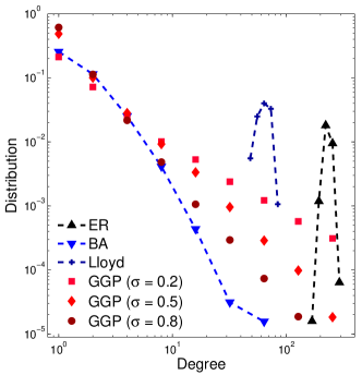
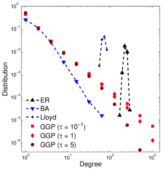
(a)	(b)
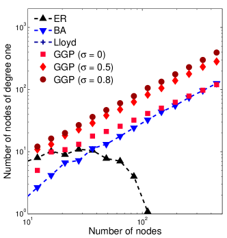
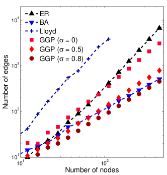
(c)	(d)

Figure 6: Examination of the GGP undirected network properties (averaging over graphs with various $\alpha$) in comparison to an Erdös Rényi $G(n,p)$ model with $p=0.05$ (ER), the preferential attachment model of (Barabási and Albert, 1999) (BA), and the nonparametric formulation of (Lloyd et al., 2012) (Lloyd). (a-b) Degree distribution on a log-log scale for (a) various values of $\sigma$ ($\tau=10^{-2}$) and (b) various values of $\tau$ ($\sigma=0.5$) for the GGP. (c) Number of nodes with degree one versus the number of nodes on a log-log scale. Note that the Lloyd method leads to dense graphs such that no node has only degree 1. (d) Number of edges versus the number of nodes. In (d) we note growth at a rate $o(n^{2})$ for our GGP graph models, and $\Theta(n^{2})$ for the Erdös Rényi and Lloyd models (dense graphs).

Interpretation of hyperparameters

Based on the properties derived and explored empirically in this section, we see that our hyperparameters have the following interpretations:

• $\boldsymbol{\sigma}$— From Figure 6(a) and (d), $\sigma$ relates to the slope of the degree distribution in its power-law regime and the overall network sparsity. Increasing $\sigma$ leads to higher power-law exponent and sparser networks.

• $\boldsymbol{\alpha}$— From Theorem 5.9, $\alpha$ provides an overall scale that affects the number of nodes and directed interactions, with larger $\alpha$ leading to larger networks.

• $\boldsymbol{\tau}$— From Figure 6(b), $\tau$ determines the exponential decay of the tails of the power-law degree distribution, with $\tau$ small looking like pure power-law. This is intuitive from the form of $\rho(dw)$ in (41), where we see that $\tau$ affects large weights more than small ones.

6 Posterior characterization and inference

In this section we target inferring the posterior distribution of the sociability parameters, $w_{i}$, restriction value $\alpha$, and CRM hyperparameters. In the special case of GGPs, our hyperparameters of interest are then the set $(\alpha,\sigma,\tau)$.

6.1 Directed multigraph and undirected simple graph

We first characterize the conditional distribution of the restricted CRM $W_{\alpha}$ given the directed graph $D_{\alpha}$ (see (22) and surrounding text). In what follows, we utilize the fact that the conditional CRM $W_{\alpha}$ given $D_{\alpha}$ can be decomposed as a sum of (i) a measure with fixed locations $\theta_{i}$ and random weights $w_{i}$, corresponding to nodes for which we observed at least one connection, and (ii) a measure with random weights and random atoms, corresponding to the remaining set of nodes. We denote the total mass of this remaining weight as $w_{\ast}$.

Theorem 6.14.

Let $(\theta_{1},\ldots,\theta_{N_{\alpha}})$, $N_{\alpha}\geq 0,$ be the set of support points of $D_{\alpha}$ such that $D_{\alpha}=\sum_{1\leq i,j\leq N_{\alpha}}n_{ij}\delta_{(\theta_{i},\theta_{j})}$. Let $m_{i}=\sum_{j=1}^{N_{\alpha}}(n_{ij}+n_{ji})>0$ for $i=1,\ldots,N_{\alpha}$. The conditional distribution of $W_{\alpha}$ given $D_{\alpha}$ is equivalent to the distribution of

$$w_{\ast}\sum_{i=1}^{\infty}\widetilde{P}_{i}\delta_{\widetilde{\theta}_{i}}+\sum_{i=1}^{N_{\alpha}}w_{i}\delta_{\theta_{i}}$$ (49)

where $\widetilde{\theta}_{i}\sim\operatorname{Unif}([0,\alpha])$, and the weights $(\widetilde{P}_{i})_{i=1,2,\ldots},$ with $\widetilde{P}_{1}>\widetilde{P}_{2}>\ldots$ and $\sum_{i=1}^{\infty}\widetilde{P}_{i}=1,$ are distributed from a Poisson-Kingman distribution (Pitman, 2003, Definition 3 p.6) with Lévy intensity $\rho$, conditional on $w_{\ast}$

$$(\widetilde{P}_{i})|w_{\ast}\sim\operatorname{PK}(\rho|w_{\ast}).$$

Finally, the weights $(w_{1},\ldots,w_{N_{\alpha}},w_{\ast})$ are jointly dependent conditional on $D_{\alpha}$, with the following posterior distribution:

$$p(w_{1},\ldots,w_{N_{\alpha}},w_{\ast}|D_{\alpha})\propto\left[\prod_{i=1}^{N_{\alpha}}w_{i}^{m_{i}}\right]e^{-\left(\sum_{i=1}^{N_{\alpha}}w_{i}+w_{\ast}\right)^{2}}\left[\prod_{i=1}^{N_{\alpha}}\rho(w_{i})\right]\times g_{\alpha}^{\ast}(w_{\ast})$$ (50)

where $g_{\alpha}^{\ast}$ is the probability density function of the random variable $W^{*}_{\alpha}=W_{\alpha}([0,\alpha])$, with Laplace transform

$$\mathbb{E}[e^{-tW^{*}_{\alpha}}]=e^{-\alpha\psi(t)}.$$ (51)

Proof 6.15.

The proof builds on the Palm formula for Poisson random measures (Prünster, 2002; James, 2002, 2005; James, Lijoi and Prünster, 2009) and is described in Appendix D.

Note that the normalized weights $(\widetilde{P}_{i})_{i=1,2,\ldots}$ and locations $(\widetilde{\theta}_{i})_{i=1,2,\ldots}$ are not likelihood identifiable, as the likelihood only brings information on the weights of the observed nodes, and on the total mass $w_{\ast}$ of the remaining nodes. Additionally, note that the conditional distribution of $(w_{1},\ldots,w_{N_{\alpha}},w_{\ast})$ given $D_{\alpha}$ does not depend on the locations $(\theta_{1},\ldots,\theta_{N_{\alpha}})$ because we considered a homogeneous CRM. This fact is important since the locations $(\theta_{1},\ldots,\theta_{N_{\alpha}})$ are typically not observed, and our algorithm outlined below will not consider these terms in the inference.

We now specialize to the special case of the GGP, for which we derive an MCMC sampler for posterior inference. Let $\phi=(\alpha,\sigma,\tau)$ be the set of hyperparameters that we also want to estimate. We will assume improper priors on those parameters:

$$p(\alpha)\propto\frac{1}{\alpha},\,\,\,p(\sigma)\propto\frac{1}{1-\sigma},\,\,\,p(\tau)\propto\frac{1}{\tau}.$$

To emphasize the dependence of the Lévy measure and pdf of the total mass $w_{*}$ on the hyperparameters, we write $\rho(w|\sigma,\tau)$ and $g_{\alpha,\sigma,\tau}^{\ast}(w_{\ast})$. We are interested in approximating the posterior $p(w_{1},\ldots,w_{N_{\alpha}},w_{\ast},\phi|(n_{ij})_{1\leq i,j\leq N_{\alpha}})$ for a directed multigraph or $p(w_{1},\ldots,w_{N_{\alpha}},w_{\ast},\phi|(z_{ij})_{1\leq i,j\leq N_{\alpha}})$ for a simple graph.

In the case of a simple graph, we will simply impute the missing directed edges in the graph. For each $i\leq j$ such that $z_{ij}=1$, we introduce latent variables $\overline{n}_{ij}=n_{ij}+n_{ji}$ with conditional distribution

$$\overline{n}_{ij}|z,w\sim\left\{\begin{array}[c]{ll}\delta_{0}&\text{if }z_{ij}=0\\ \text{tPoisson}(2w_{i}w_{j})&\text{if }z_{ij}=1,\text{ }i\neq j\\ \text{tPoisson}(w_{i}^{2})&\text{if }z_{ii}=1,\text{ }i=j,\end{array}\right.$$ (52)

where tPoisson($\lambda$) is the zero-truncated Poisson distribution with pdf

$$\frac{k^{\lambda}\exp(-\lambda)}{(1-\exp(-\lambda))k!}\text{, for }k=1,2,\ldots$$

By convention, we set $\overline{n}_{ij}=\overline{n}_{ji}$ for $j<i$ and $m_{i}=\sum_{j=1}^{N_{\alpha}}\overline{n}_{ij}$.

For efficient exploration of the target posterior, we propose using a Hamiltonian Monte Carlo (HMC) algorithm (Duane et al., 1987; Neal, 2011) within Gibbs to update the weights $(w_{1},\ldots,w_{N_{\alpha}})$. The HMC step requires computing the gradient of the log-posterior, which in our case, letting $\omega_{i}=\log w_{i}$, is given by

$$\left[\nabla_{\omega_{1:N_{\alpha}}}\log p(\omega_{1:N_{\alpha}},w_{\ast}|D_{\alpha})\right]_{i}=m_{i}-\sigma-w_{i}\left(\tau+2\sum_{j=1}^{N_{\alpha}}w_{j}+2w_{\ast}\right).$$ (53)

For the update of the total mass $w_{\ast}$ and hyperparameters $\phi$, we use a Metropolis-Hastings step. Note that, except in some particular cases ($\sigma=0,\frac{1}{2}$), the density $g_{\alpha,\sigma,\tau}^{\ast}(w_{\ast})$ does not admit any analytical expression. We therefore use a specific proposal for $w_{\ast}$ based on exponential tilting of $g_{\alpha,\sigma,\tau}^{\ast}$ that alleviates the need to evaluate this pdf in the Metropolis-Hasting ratio (see details in Appendix E). To summarize, the MCMC sampler is defined as follows:

1. Update the weights $(w_{1},\ldots,w_{N_{\alpha}})$ given the rest using an HMC update

2. Update the total mass $w_{\ast}$ and hyperparameters $\phi=(\alpha,\sigma,\tau)$ given the rest using a Metropolis-Hastings update

3. [Undirected graph] Update the latent counts $(\overline{n}_{ij})$ given the rest using the conditional distribution (52) or a Metropolis-Hastings update

Note that the computational bottlenecks lie in steps 1 and 3, which roughly scale linearly in the number of nodes/edges, respectively, although one can parallelize step 3 over edges. If $L$ is the number of leapfrog steps in the HMC algorithm, $n_{\text{iter}}$ the number of MCMC iterations, the overall complexity is in $O(n_{\text{iter}}(LN_{\alpha}+N_{\alpha}^{(e)}))$. We show in Section 7 that the algorithm scales well to large networks with hundreds of thousands of nodes and edges. To efficiently scale HMC to even larger collections of nodes/edges, one can deploy the methods of Chen, Fox and Guestrin (2014).

6.2 Bipartite graph

For the bipartite graph case, the posterior characterization follows as proposed by Caron (2012). However, our proposed data augmentation is different and leads to a simpler form for the sampler.

Theorem 6.16.

Let $(\theta_{1},\ldots,\theta_{N_{\alpha}})$, $(\theta_{1}^{\prime},\ldots,\theta_{N_{\alpha}^{\prime}}^{\prime})$ with $N_{\alpha},N_{\alpha}^{\prime}\geq 0,$ be the set of support points of $D_{\alpha}$ and thus $D_{\alpha}=\sum_{1\leq i,j\leq N_{\alpha}}n_{ij}\delta_{(\theta_{i},\theta_{j}^{\prime})}$. Let $m_{i}=\sum_{j=1}^{N_{\alpha}^{\prime}}n_{ij}$ and $m_{j}^{\prime}=\sum_{i=1}^{N_{\alpha}}n_{ij}$ The conditional distribution of $W_{\alpha}$ given $D_{\alpha},W_{\alpha}^{\prime}$ is equivalent to the distribution of

$$\widetilde{W}+\sum_{i=1}^{N_{\alpha}}w_{i}\delta_{\theta_{i}}$$ (54)

where $(w_{1},\ldots,w_{N_{\alpha}})$ are independent of $\widetilde{W}$ with

$$p(w_{i}|D_{\alpha},W_{\alpha}^{\prime})\propto w_{i}^{m_{i}}e^{-w_{i}\left(\sum_{j=1}^{N_{\alpha}^{\prime}}w_{j}^{\prime}+w_{\ast}^{\prime}\right)}\rho(w_{i})$$ (55)

and $\widetilde{W}\sim\operatorname{CRM}(\widetilde{\rho},\lambda_{\alpha})$ is a CRM with exponentially tilted Lévy intensity

$$\widetilde{\rho}(w)=\rho(w)e^{-w\left(\sum_{j=1}^{N_{\alpha}^{\prime}}w_{j}^{\prime}+w_{\ast}^{\prime}\right)}.$$ (56)

In particular, for the generalized gamma process, we have

$$w_{i}|D_{\alpha},W_{\alpha}^{\prime}\sim\operatorname*{Gamma}\left(m_{i}-\sigma,\tau+\sum_{j=1}^{N_{\alpha}^{\prime}}w_{j}^{\prime}+w_{\ast}^{\prime}\right)$$ (57)

and the total mass $w_{\ast}$ of $\widetilde{W}$ is distributed from an exponentially tilted stable distribution with pdf

$$p(w_{\ast}|\text{rest})=\frac{e^{-w_{\ast}\left(\sum_{j=1}^{N_{\alpha}^{\prime}}w_{j}^{\prime}+w_{\ast}^{\prime}\right)}g_{\alpha}(w_{\ast})}{e^{-\psi\left(\sum_{j=1}^{N_{\alpha}^{\prime}}w_{j}^{\prime}+w_{\ast}^{\prime}\right)}},$$ (58)

from which one can sample exactly (Devroye, 2009; Hofert, 2011). Additionally, the marginal likelihood is expressed as

$$\mathbb{E}_{W_{\alpha}}[p(D_{\alpha}|W_{\alpha}^{\prime})]=e^{-\alpha\psi\left(\sum_{j=1}^{N_{\alpha}^{\prime}}w_{j}^{\prime}+w_{\ast}^{\prime}\right)}\alpha^{N_{\alpha}}\prod_{i=1}^{N_{\alpha}}\kappa\left(m_{i},\sum_{j=1}^{N_{\alpha}^{\prime}}w_{j}^{\prime}+w_{\ast}^{\prime}\right)d\theta_{i},$$ (59)

where $\kappa(n,z)=\int_{0}^{\infty}w^{n}\exp(-zw)\rho(w)dw.$

Proof 6.17.

The proof is described by Caron (2012) and in Appendix D for completeness.

Let $\phi=(\alpha,\sigma,\tau)$ and $\phi^{\prime}=(\alpha^{\prime},\sigma^{\prime})$ be, respectively, the parameters of the Lévy intensity of $W$ and $W^{\prime}$. To preserve identifiability, we set the parameter $\tau^{\prime}$ to $1$. The MCMC sampler for approximating $p(w_{1:N_{\alpha}},w_{\ast},w_{1:N_{\alpha}^{\prime}}^{\prime},w_{\ast}^{\prime},\phi,\phi^{\prime}|Z_{\alpha})$ iterates as follows:

1. Update $\alpha,\sigma,\tau$ given $w_{1:N_{\alpha}^{\prime}}^{\prime}$ using a Metropolis-Hastings step with acceptance ratio calculated with (59)

2. Update $w_{1:N_{\alpha}}$ given $(w_{1:N_{\alpha}^{\prime}}^{\prime},w_{\ast}^{\prime},\alpha,\sigma,\tau)$ using (57)

3. Update $w_{\ast}$ given $(w_{1:N_{\alpha}^{\prime}}^{\prime},w_{\ast}^{\prime},\alpha,\sigma,\tau)$ using (58)

4. Update the latent $n_{ij}$ given $w_{1:N_{\alpha}^{\prime}}^{\prime},w_{1:N_{\alpha}}$ as

   $$n_{ij}|z,w,w^{\prime}\sim\left\{\begin{array}[c]{ll}\delta_{0}&\text{if }z_{ij}=0\\ \text{tPoisson}(w_{i}w_{j}^{\prime})&\text{if }z_{ij}=1\end{array}\right.$$

The model is symmetric in $(w,w^{\prime})$, so the first three steps can be repeated for updating $(\alpha^{\prime},\sigma^{\prime},\tau^{\prime},w_{1:N_{\alpha}^{\prime}}^{\prime},w_{\ast}^{\prime})$. Full algorithmic details are given in Appendix E.

7 Experiments

7.1 Simulated data

We first study the convergence of the MCMC algorithm on simulated data where the graph is simulated from our model. We simulate a GGP undirected graph with parameters $\alpha=300,\sigma=0.5,\tau=1$. Note that we are in the sparse regime. The sampled graph has 13,995 nodes and 76,605 edges. We run 3 MCMC chains each with 40,000 iterations and with different initial values. $L=10$ leapfrog steps are used, and the stepsize of the leapfrog algorithm is adapted during the first 10,000 iterations so as to obtain an acceptance rate of 0.6. Standard deviations of the random walk Metropolis-Hastings for $\log\tau$ and $\log(1-\sigma)$ are set to 0.02. It takes 10 minutes with Matlab on a standard computer (CPU@3.10GHz, 4 cores) to run the 3 chains successively. Trace plots of the parameters $\alpha$, $\sigma$, $\tau$ and $w_{*}$ are given in Figure 7. The potential scale factor reduction (Brooks and Gelman, 1998; Gelman et al., 2014) is computed for all 13,999 parameters $(w_{1:N_{\alpha}},w_{*},\alpha,\sigma,\tau)$ and has a maximum value of 1.01, indicating convergence of the algorithm. This is rather remarkable as the MCMC sampler actually samples from a target distribution of dimension 13,995+76,605+4=90,604. Posterior credible intervals of the sociability parameters $w_{i}$ of the nodes with highest degrees and log-sociability parameters $\log w_{i}$ of the nodes with lowest degrees are displayed in Figure 8(a) and (b), respectively, showing the ability of the method to accurately recover sociability parameters of both low and high degree nodes.

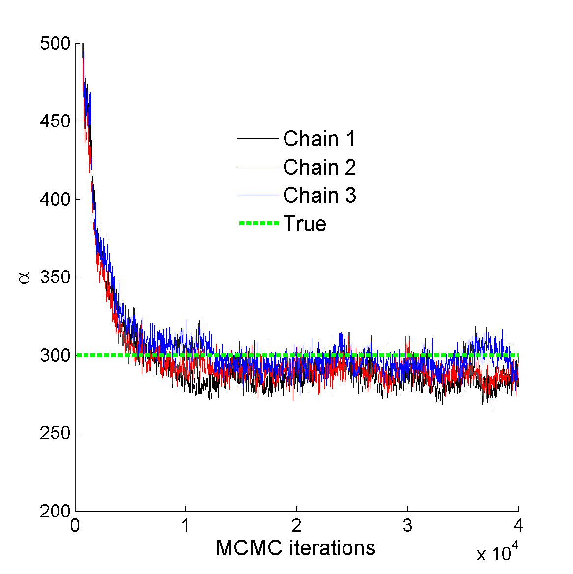
(a) $\alpha$

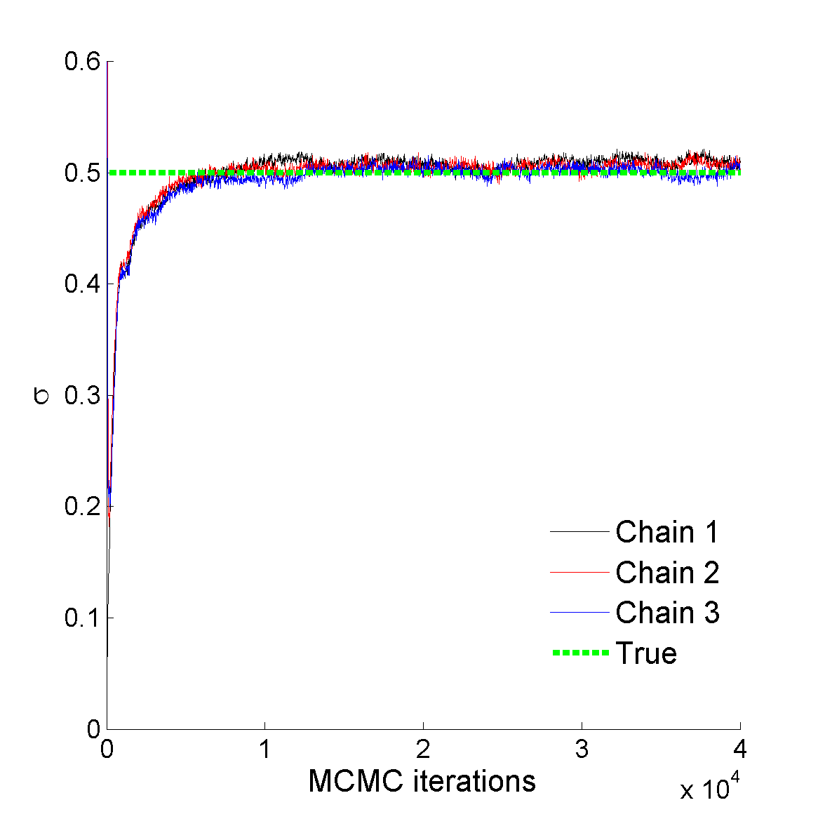
(b) $\sigma$

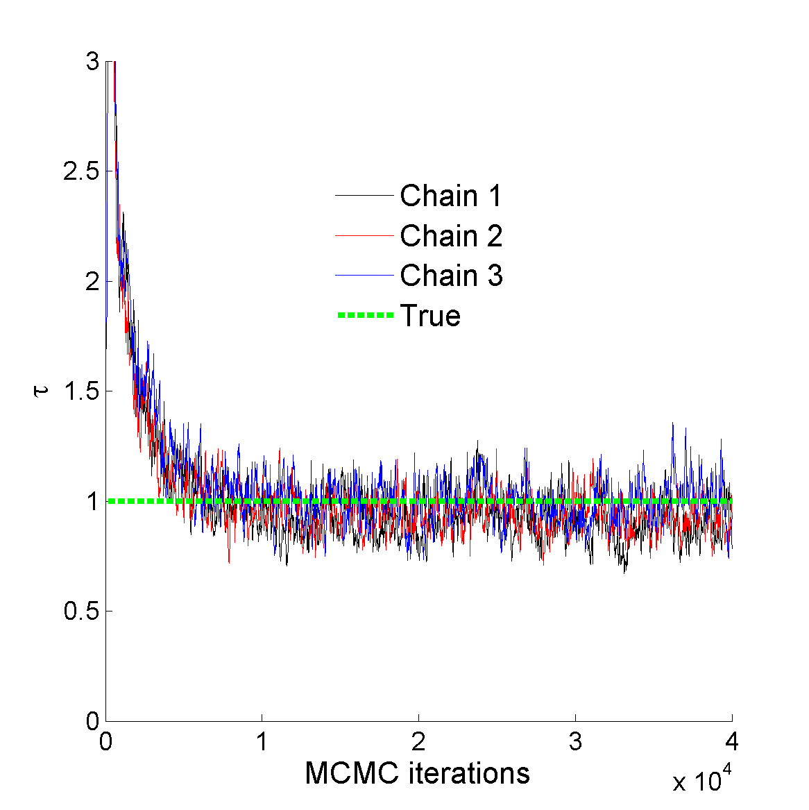
(c) $\tau$

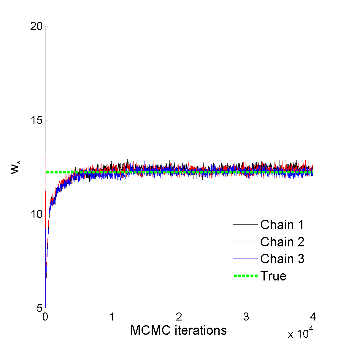
(d) $w_{*}$

Figure 7: MCMC trace plots of parameters (a) $\alpha$ (b) $\sigma$, (c) $\tau$ and (d) $w_{*}$ for a graph generated from a GGP model with parameters $\alpha=300,\sigma=0.5,\tau=1$.

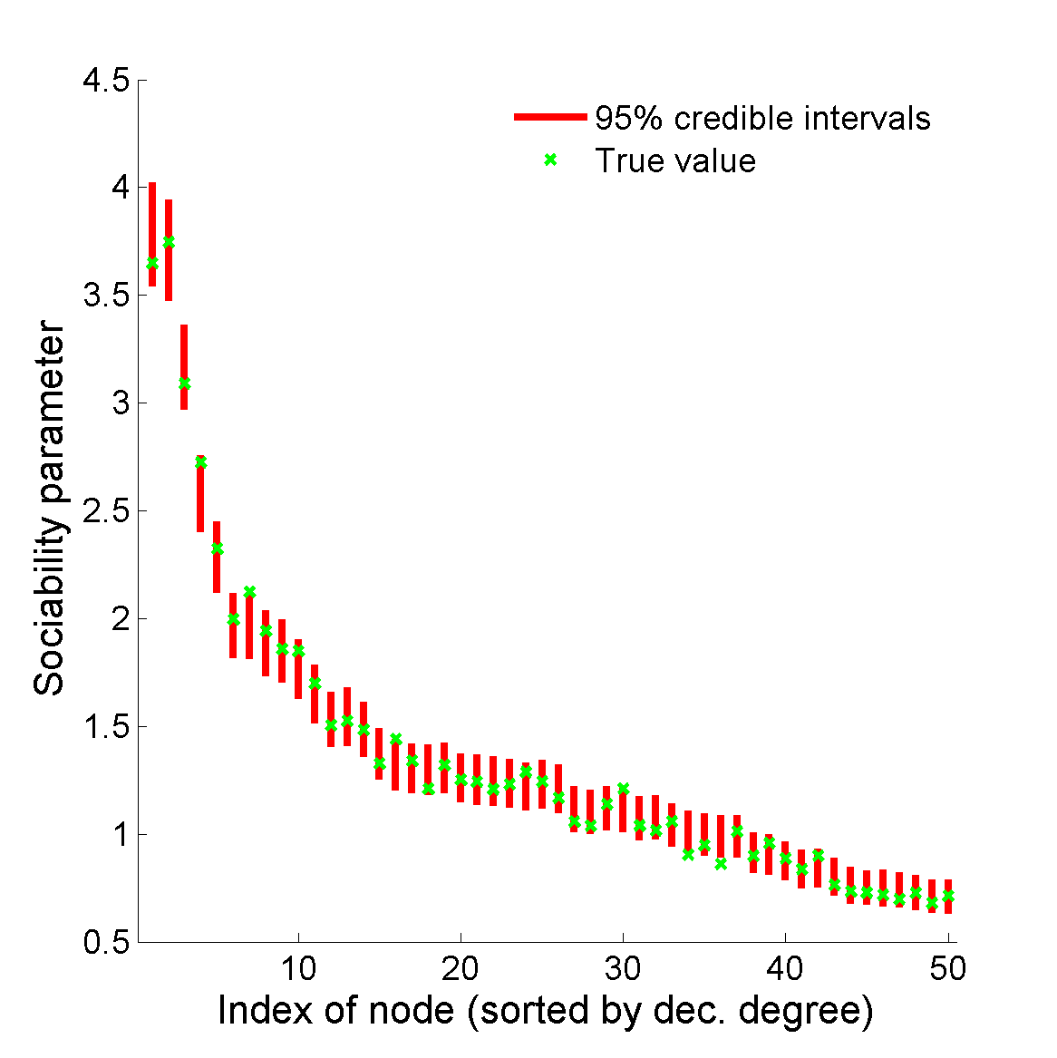
(a) 50 nodes with highest degree

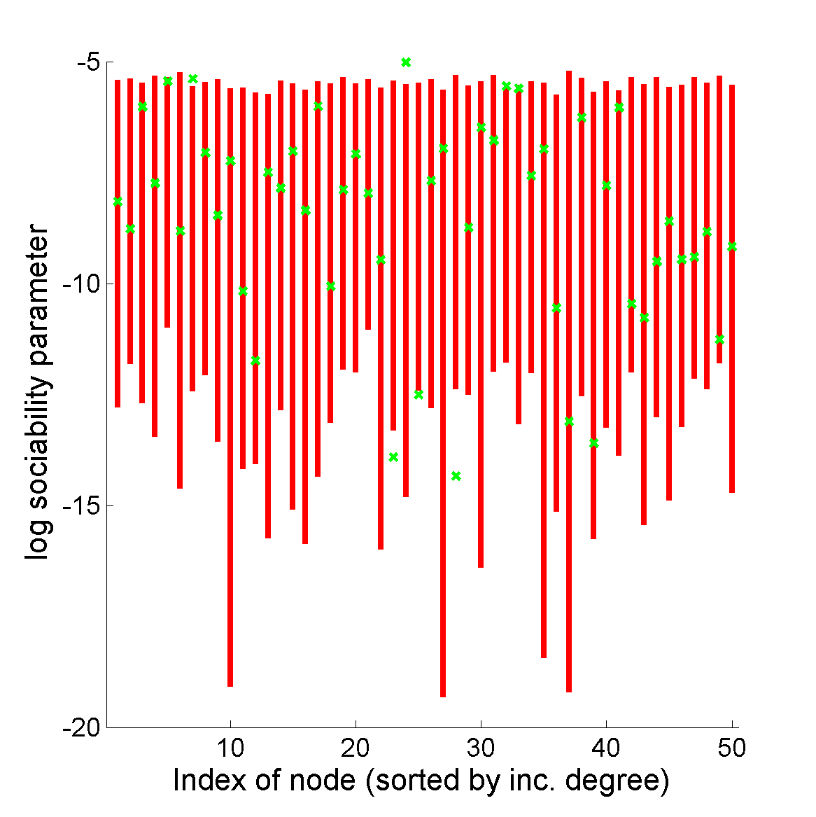
(b) 50 nodes with lowest degree

Figure 8: 95 % posterior intervals of (a) the sociability parameters $w_{i}$ of the 50 nodes with highest degree and (b) the log-sociability parameter $\log w_{i}$ of the 50 nodes with lowest degree, for a graph generated from a GGP model with parameters $\alpha=300,\sigma=0.5,\tau=1$. True values are represented by a green star.

To show the versatility of the GGP graph model, we now examine our approach when the observed graph is actually generated from an Erdös-Rényi model with $n=1,000$ and $p=0.01$. The generated graph has 1,000 nodes and 5,058 edges. We ran 3 MCMC chains with the same specifications as above. In this dense-graph regime, the following transformation of our parameters $\alpha$, $\sigma$ and $\tau$ is more informative: $\varsigma_{1}=-\frac{\alpha}{\sigma}\tau^{\sigma}$, $\varsigma_{2}=-\frac{\sigma}{\tau}$ and $\varsigma_{3}=-\frac{\sigma}{\tau^{2}}$. When $\sigma<0$, $\varsigma_{1}$ corresponds to the expected number of nodes, $\varsigma_{2}$ to the mean of the sociability parameters and $\varsigma_{3}$ to their variance (see Section 5.3). In contrast, the parameters $\sigma$ and $\tau$ are only weakly identifiable in this case. The potential scale reduction factor is computed on $(w_{1:N_{\alpha}},w_{*},\varsigma_{1},\varsigma_{2},\varsigma_{3})$, and its maximum value is 1.01, indicating convergence. Trace plots are shown in Figure 9 for $\varsigma_{1}$, $\varsigma_{2}$, $\varsigma_{3}$ and $w_{*}$. The value of $\varsigma_{1}$ converges around the true number of nodes, $\varsigma_{2}$ to the true sociability parameter $\sqrt{-\frac{1}{2}\log(1-p)}$ (constant across nodes for the Erdös-Rényi model), while $\varsigma_{3}$ is close to zero as the variance over the sociability parameters is very small. The total mass is very close to zero, indicating that there are no nodes with degree zero.

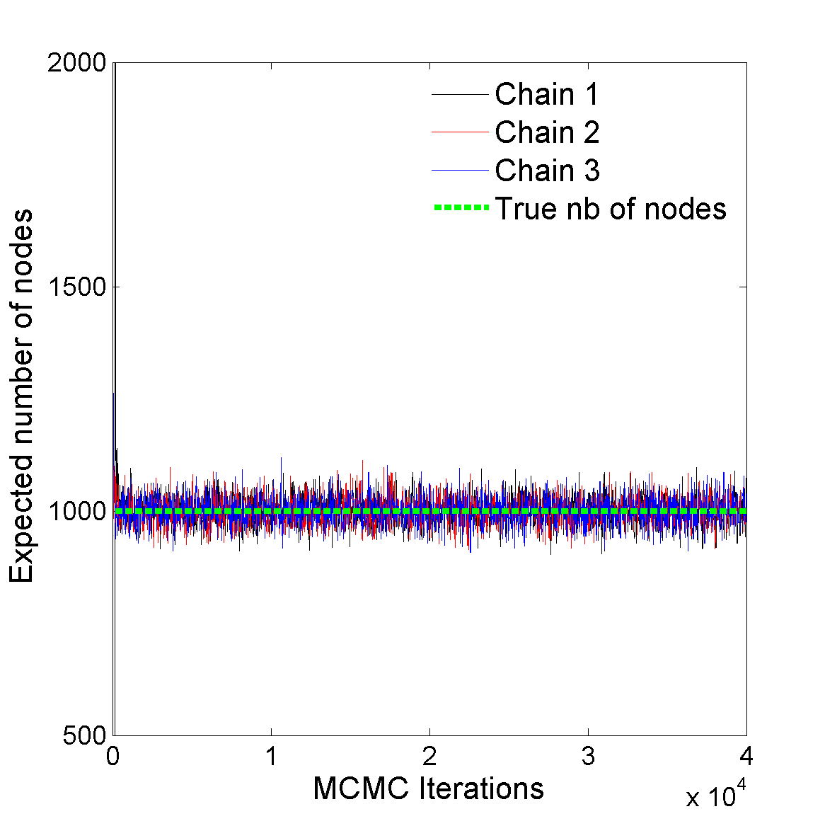
(a) $\varsigma_{1}=-\frac{\alpha}{\sigma}\tau^{\sigma}$

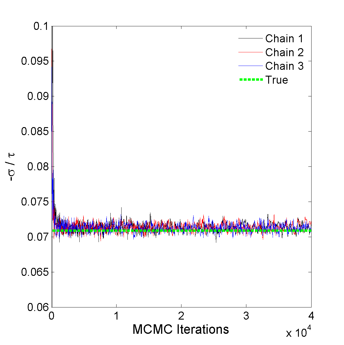
(b) $\varsigma_{2}=-\frac{\sigma}{\tau}$

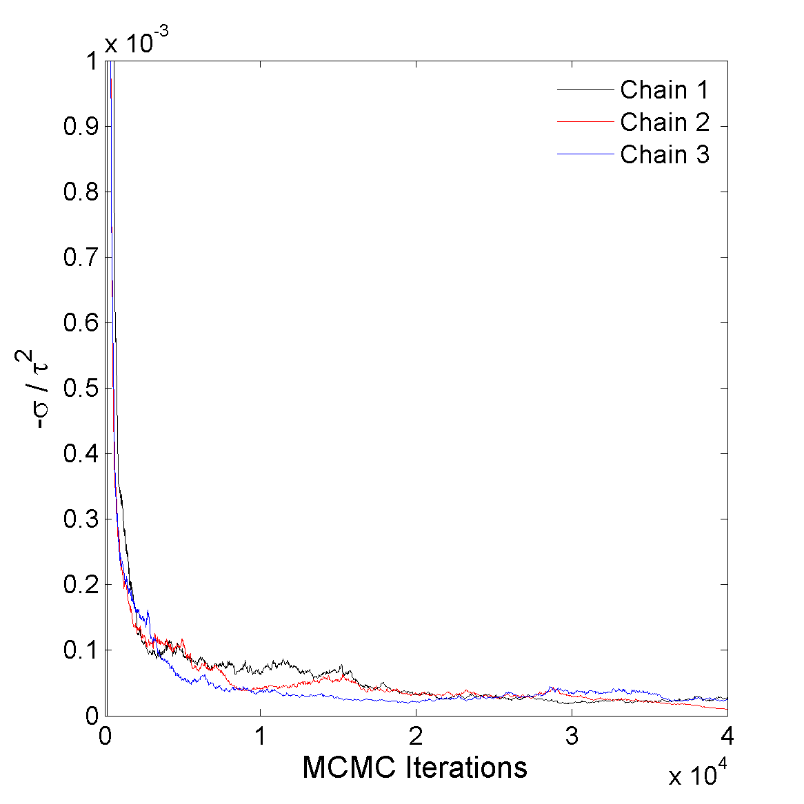
(c) $\varsigma_{3}=-\frac{\sigma}{\tau^{2}}$

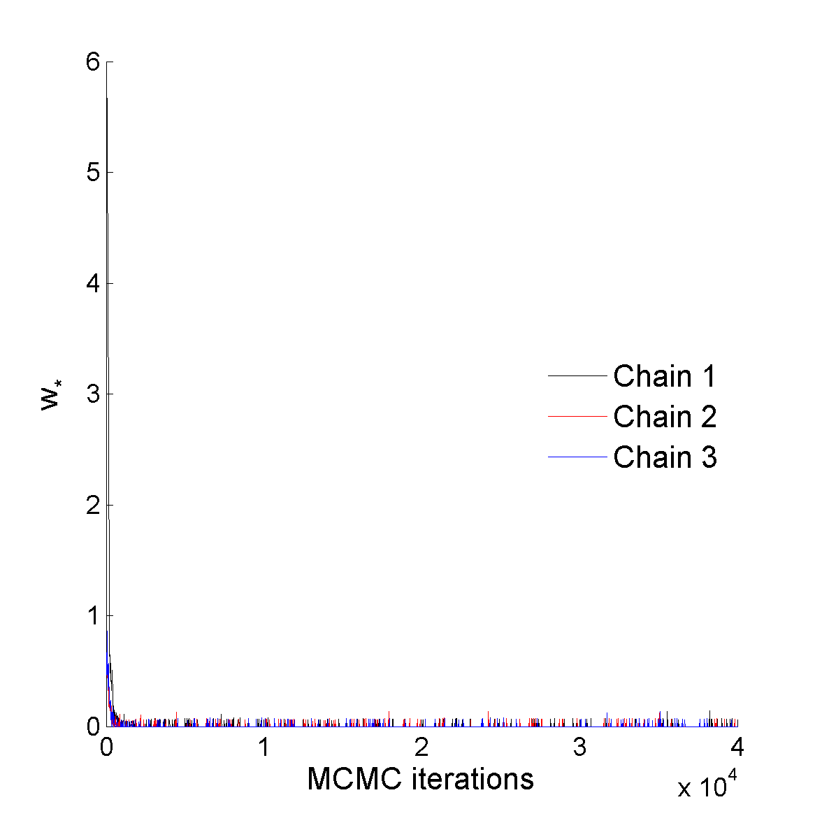
(d) $w_{*}$

Figure 9: MCMC trace plots of parameters (a) $\varsigma_{1}$ (b) $\varsigma_{2}$, (c) $\varsigma_{3}$, (d) $w_{*}$ for a graph generated from an Erdös-Rényi model with parameters $n=1000,p=0.01$.

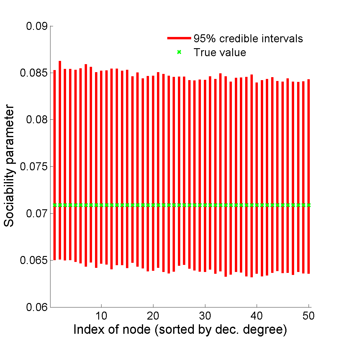
(a) Nodes with highest degree

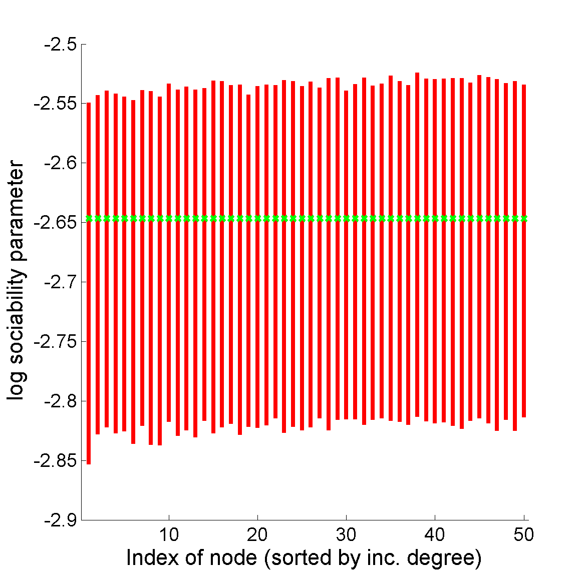
(b) Nodes with lowest degree

Figure 10: 95% posterior intervals of (a) sociability parameters $w_{i}$ of the 50 nodes with highest degree and (b) log-sociability parameters $\log w_{i}$ of the 50 nodes with lowest degree, for a graph generated from an Erdös-Rényi model with parameters $n=1000,p=0.01$. In this case, all nodes have the same true sociability parameter $\sqrt{-\frac{1}{2}\log(1-p)}$, represented by a green star.

7.2 Testing for sparsity of real-world graphs

We now turn to using our methods to test whether a given graph is sparse or not. Such testing based on a single given graph is notoriously challenging as sparsity relates to the asymptotic behavior of the graph. Measures of sparsity from finite graphs exist, but can be costly to implement (Nešetřil and Ossona de Mendez, 2012). Based on our GGP-based formulation and associated theoretical results described in Section 5, we propose the following test:

$$H_{0}:\sigma<0\,\,\,\mbox{ vs }\,\,\,H_{1}:\sigma\geq 0.$$

In our experiments, we again consider a GGP-based graph model with improper priors on the unknown parameters $(\alpha,\sigma,\tau)$, as described in Section 6. We aim at reporting $\Pr(H_{1}|z)=\Pr(\sigma>0|z)$ based on a set of observed connections $(z)$, which can be directly approximated from the MCMC output. We consider 12 different datasets:

• facebook107: Social circles from Facebook (McAuley and Leskovec, 2012)

• polblogs: Political blogosphere (Feb. 2005) (Adamic and Glance, 2005)

• USairport: US airport connection network in 2010 (Colizza, Pastor-Satorras and Vespignani, 2007)

• UCirvine: Social network of students at University of California, Irvine (Opsahl and Panzarasa, 2009)

• yeast: Yeast protein interaction network (Bu et al., 2003)

• USpower: Network of high-voltage power grid in the Western States of the United States of America (Watts and Strogatz, 1998)

• IMDB: Actor collaboration network based on acting in the same movie

• cond-mat1: Co-authorship network (Newman, 2001), based on preprints posted to Condensed Matter of Arxiv between 1995 and 1999; obtained from the bipartite preprints/authors network using a one-mode projection

• cond-mat2: As in cond-mat1, but using Newman’s projection method

• Enron: Enron collaboration network from multigraph email network

• internet: Connectivity of internet routers

• www: Linked www pages in the nd.edu domain

The sizes of the different datasets are given in Table 2 and range from a few hundred nodes/edges to a million. The adjacency matrices for these networks are plotted in Figure 11 and empirical degree distributions in Figure 14 (red).

Table 2: Size of real-world datasets and posterior probability of sparsity.

Name	Nb nodes	Nb edges	Time	$\Pr(H_{1}|z)$	99% CI $\sigma$
			(min)
facebook107	1,034	26,749	1	0.000	$[-1.057,-0.819]$
polblogs	1,224	16,715	1	0.000	$[-0.348,-0.202]$
USairport	1,574	17,215	1	1.000	$[~{}0.099,~{}0.181]$
UCirvine	1,899	13,838	1	0.000	$[-0.141,-0.017]$
yeast	2,284	6,646	1	0.280	$[-0.093,0.054]$
USpower	4,941	6,594	1	0.000	$[-4.837,-3.185]$
IMDB	14,752	38,369	2	0.000	$[-0.244,-0.173]$
cond-mat1	16,264	47,594	2	0.000	$[-0.945,-0.837]$
cond-mat2	7,883	8,586	1	0.000	$[-0.176,-0.022]$
Enron	36,692	183,831	7	1.000	$[~{}0.201,~{}0.221]$
internet	124,651	193,620	15	0.000	$[-0.201,-0.171]$
www	325,729	1,090,108	132	1.000	$[0.262,0.298]$

We ran 3 MCMC chains for 40,000 iterations with the same specifications as above and report the estimate of $\Pr(H_{1}|z)$ and 99% posterior credible intervals of $\sigma$ in Table 2; we additionally provide runtimes. Figure 12 and Figure 13 show MCMC traces and posterior histograms, respectively, for the sparsity parameter $\sigma$ for the different datasets. Many of the smaller networks fail to provide evidence of sparsity. These graphs may indeed be dense; for example, our facebook107 dataset represents a small social circle that is likely highly interconnected and the polblogs dataset represents two tightly connected political parties. Three of the datasets (USairport, Enron, www) are clearly inferred as sparse; note that two of these datasets are in the top three largest networks considered, where sparsity is more commonplace. In the remaining large, but inferred-dense network, internet, there is not enough evidence under our test that the network is not dense. This may be due to the presence of dense subgraphs or spots (e.g., spatially proximate routers may be highly interconnected, but sparsely connected outside the group) (Borgs et al., 2014). This relates to the idea of community structure, though not every node need be associated with a community. As in many sparse network models that assume no dense spots (Bollobás and Riordan, 2009; Wolfe and Olhede, 2013), our approach does not explicitly model such effects. Capturing such structure remains a direction of future research likely feasible within our generative framework, though our current method has the benefit of simplicity with three hyperparameters tuning the network properties. Finally, we note in Table 2 that our analyses finish in a remarkably short time despite the code base being implemented in Matlab on a standard desktop machine, without leveraging possible opportunities for parallelizing and otherwise scaling some components of the sampler (see Section 6 for a discussion.)

To assess our fit to the empirical degree distributions, we use the methods described in Section 4.4 to simulate 5000 graphs from the posterior predictive and compare to the observed graph degrees in Figure 14. In all cases, we see a reasonably good fit. For the largest networks, Figure 14(j)-(l), we see a slight underestimate of the tail of the distribution; that is, we do not capture as many high-degree nodes as truly present. This may be because these graphs exhibit a power-law behavior, but only after a certain cutoff (Clauset, Shalizi and Newman, 2009), which is not an effect explicitly modeled by our framework. Likewise, this cutoff might be due to the presence of dense spots. In contrast, we capture power-law behavior with possible exponential cutoff in the tail. We see a similar trend for cond-mat1, but not cond-mat2. Based on the bipartite articles-authors graph, cond-mat1 uses the standard one-mode projection and sets a connection between two authors who have co-authored a paper; this projection clearly creates dense spots in the graph. On the contrary, cond-mat2 uses Newman’s projection method (Newman, Strogatz and Watts, 2001). This method constructs a weighted undirected graph by counting the number of papers co-authored by two scientists, where each count is normalized by the number of authors on the paper. To construct the undirected graph, we set an edge if the weight is equal or greater than 1; cond-mat1 and cond-mat2 thus have a different number of edges and nodes, as only nodes with at least one connection are considered. It is interesting to note that the projection method used for the cond-mat dataset has a clear impact on the sparsity of the resulting graph, cond-mat2 being less dense than cond-mat1 (see Figure 14(h)-(i)). The degree distribution for cond-mat1 is similar to that of internet, thus inheriting the same issues previously discussed. Overall, it appears our model better captures homogeneous power-law behavior with possible exponential cutoff in the tails than it does a graph with perhaps structured dense spots or power-law-after-cutoff behavior.

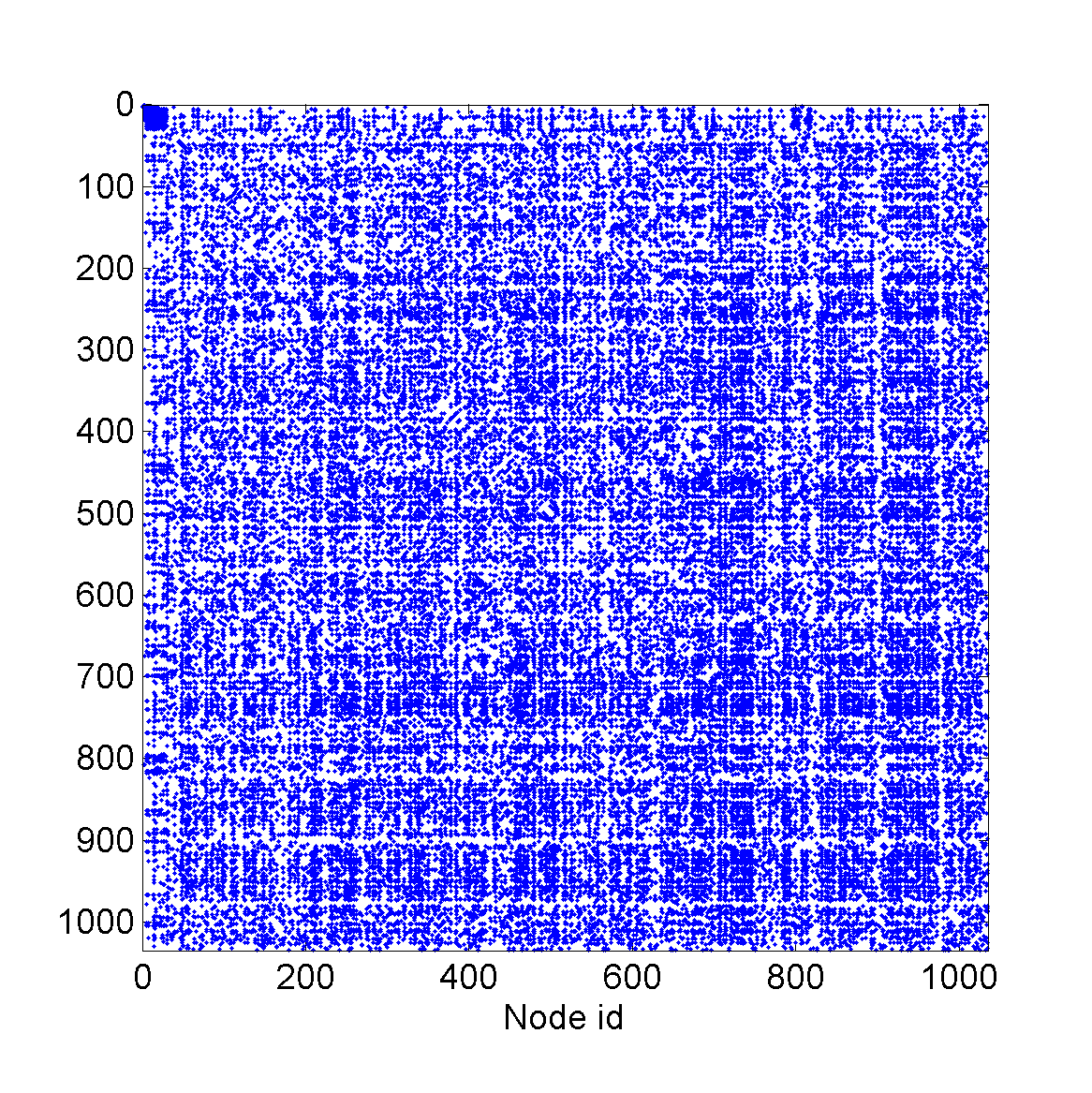
(a) facebook107

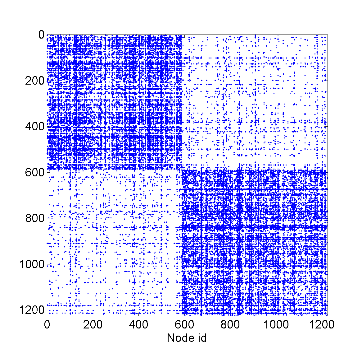
(b) polblogs

(c) USairport

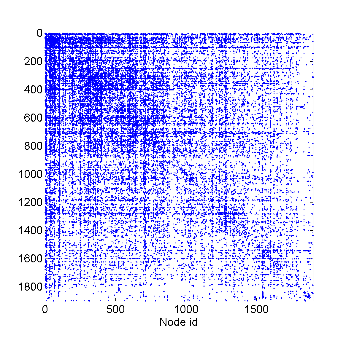
(d) UCirvine

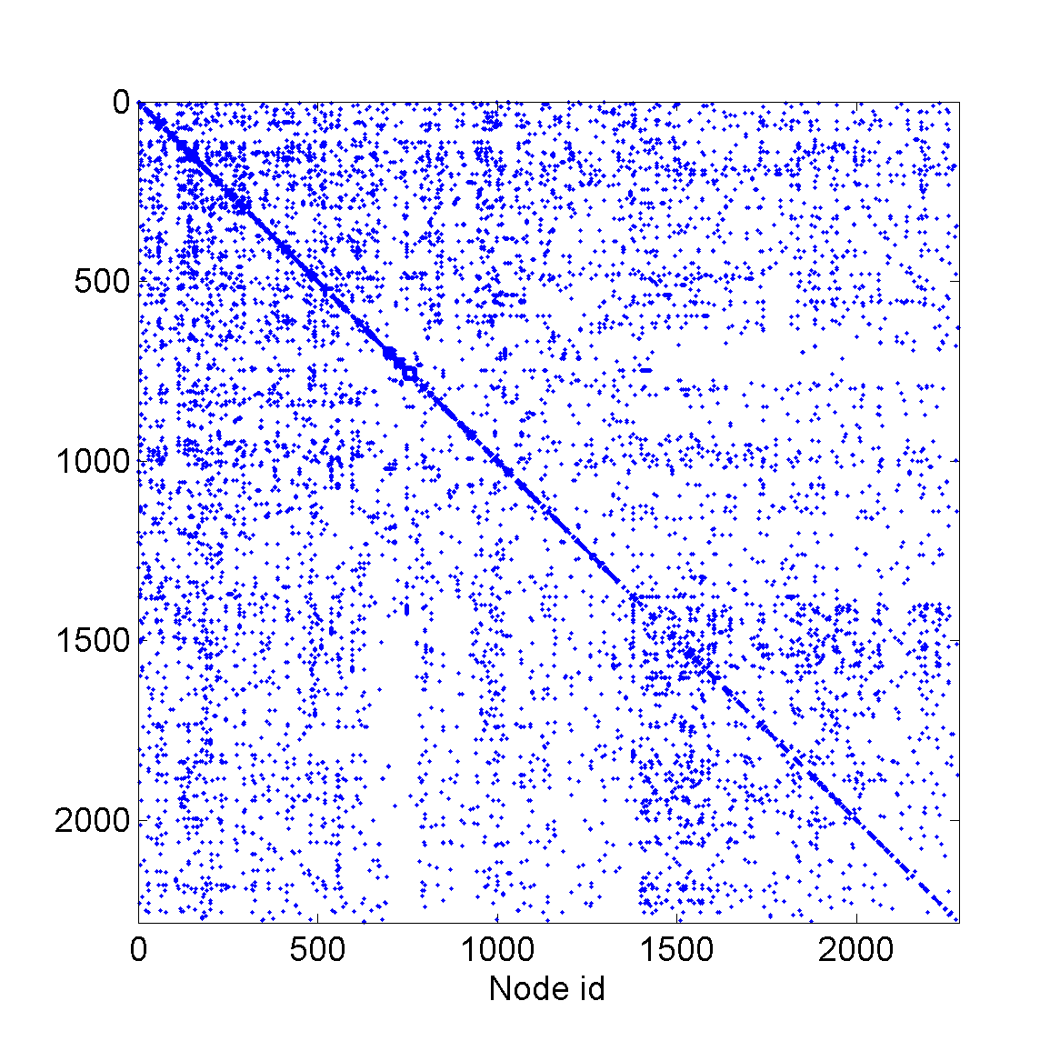
(e) yeast

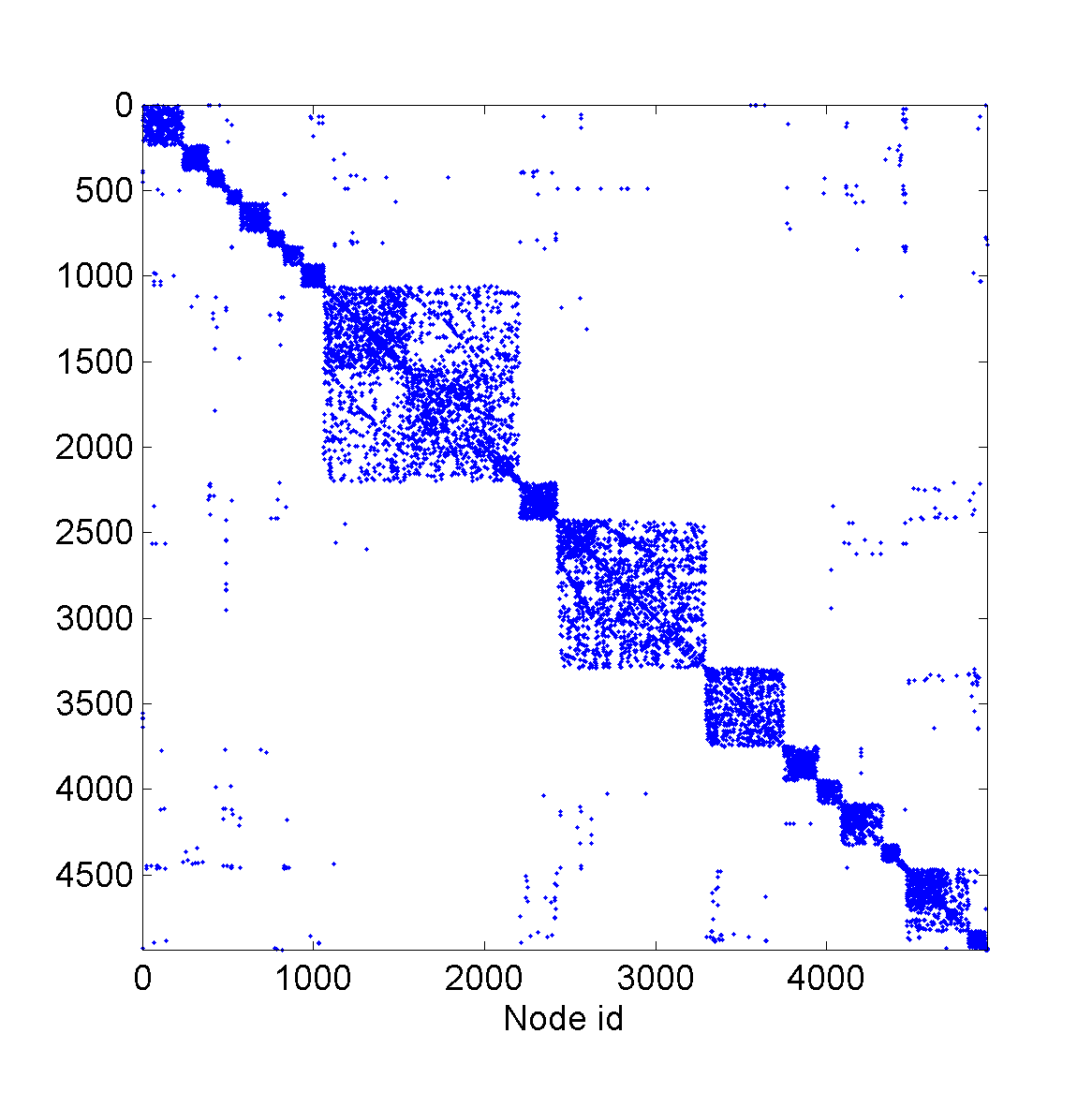
(f) USpower

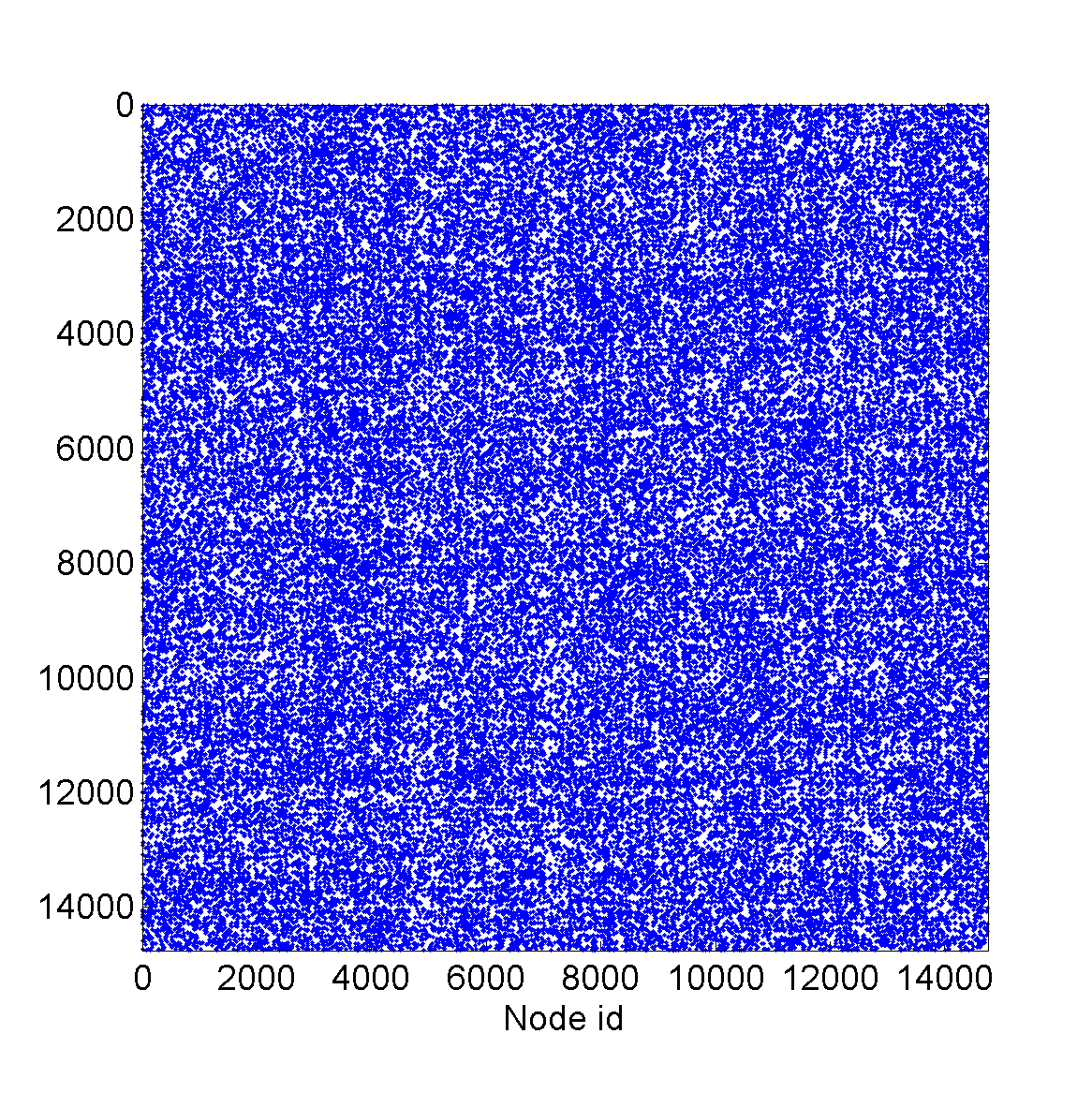
(g) IMDB

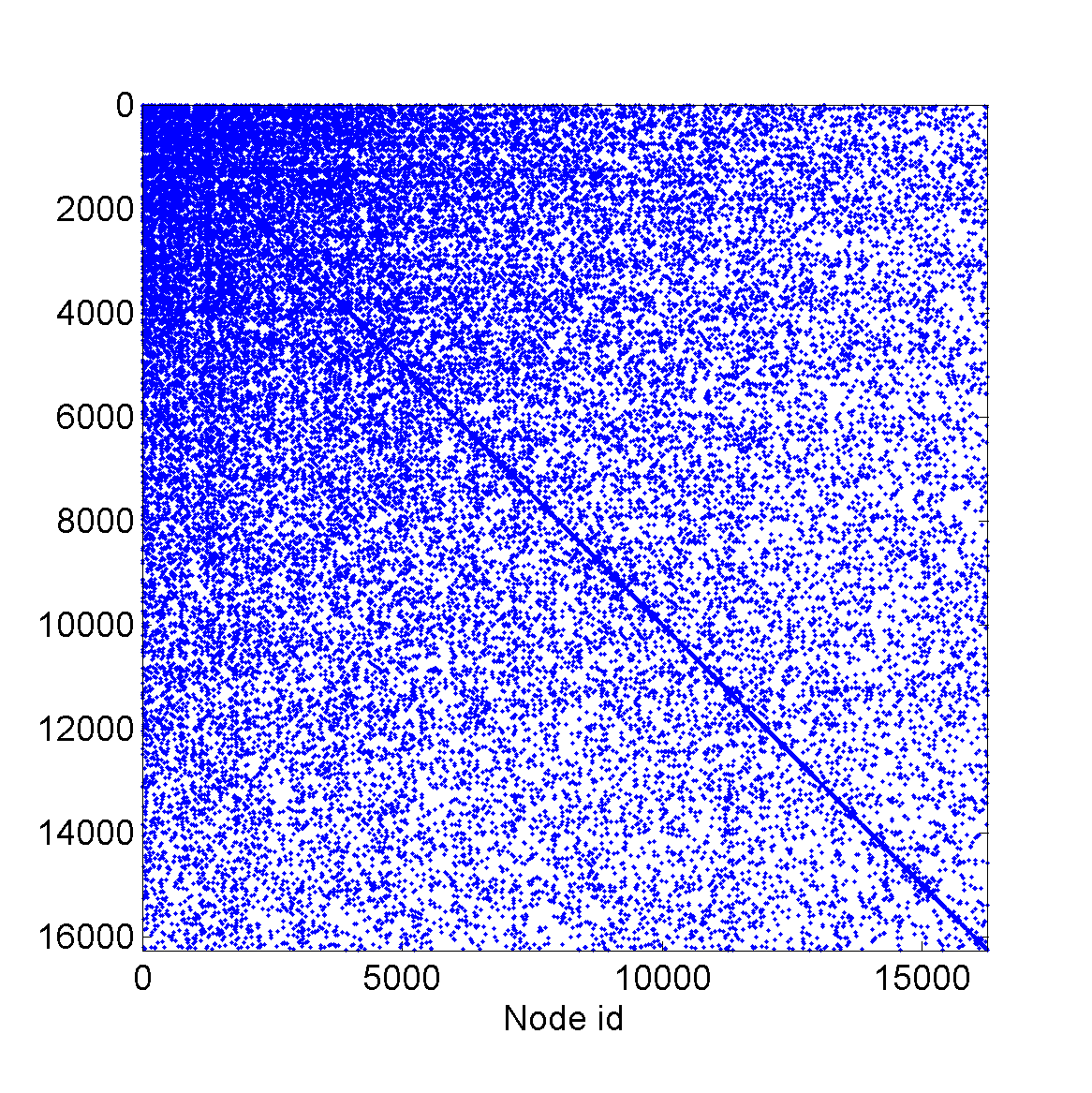
(h) cond-mat1

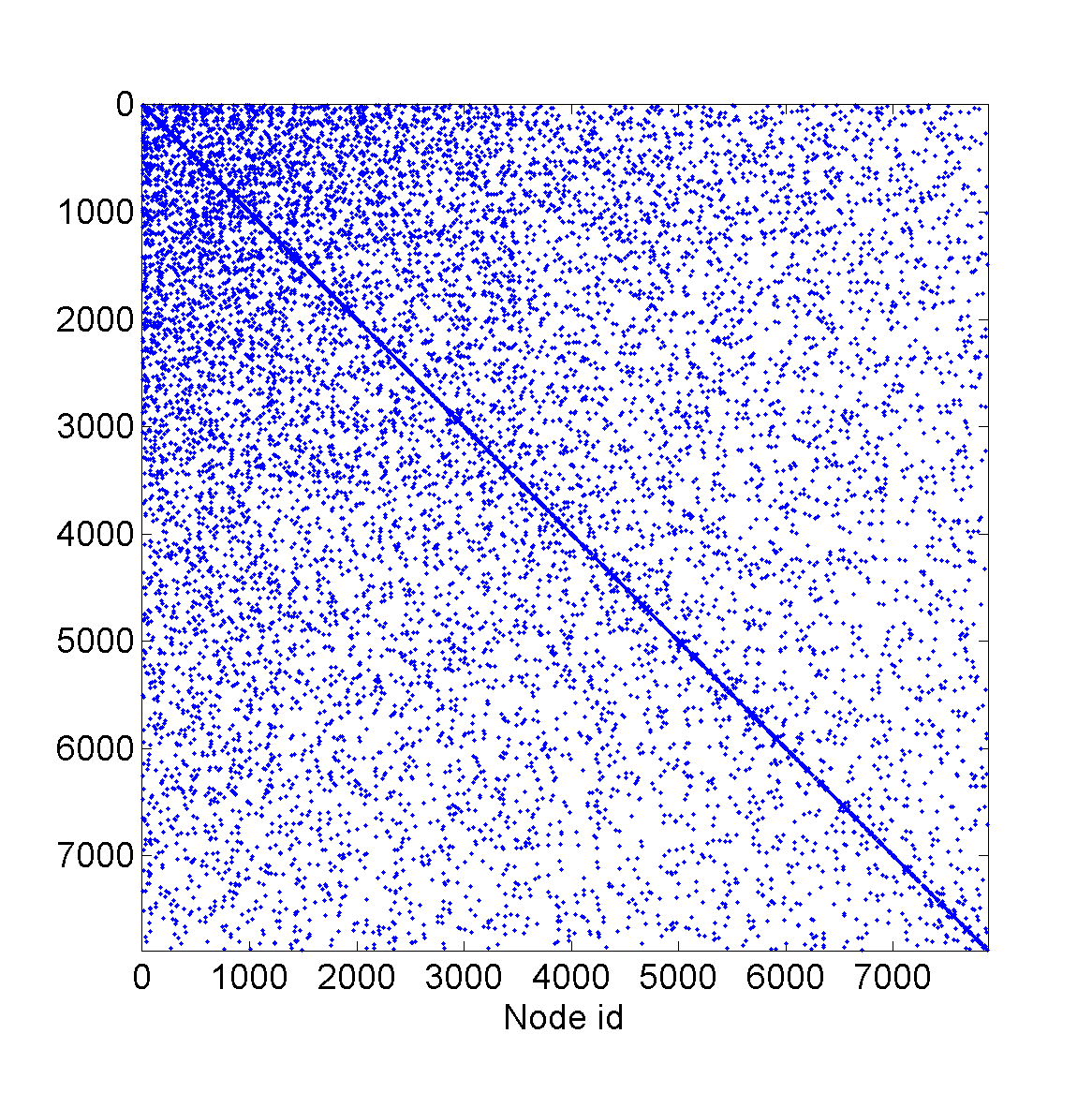
(i) cond-mat2

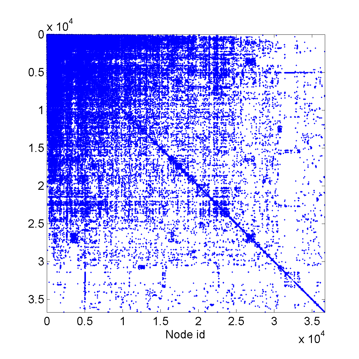
(j) enron

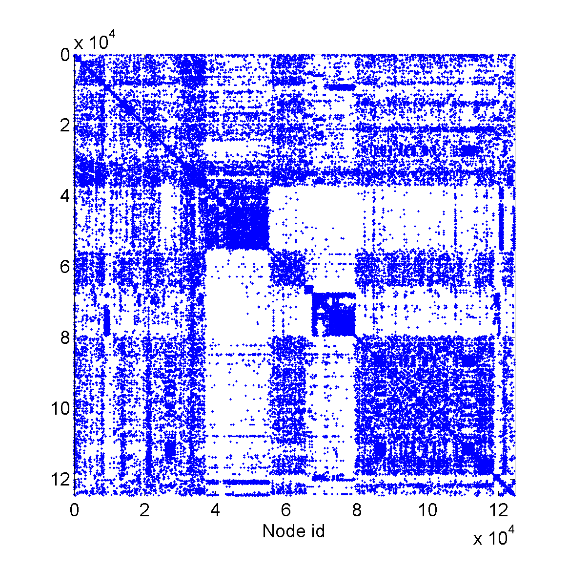
(k) internet

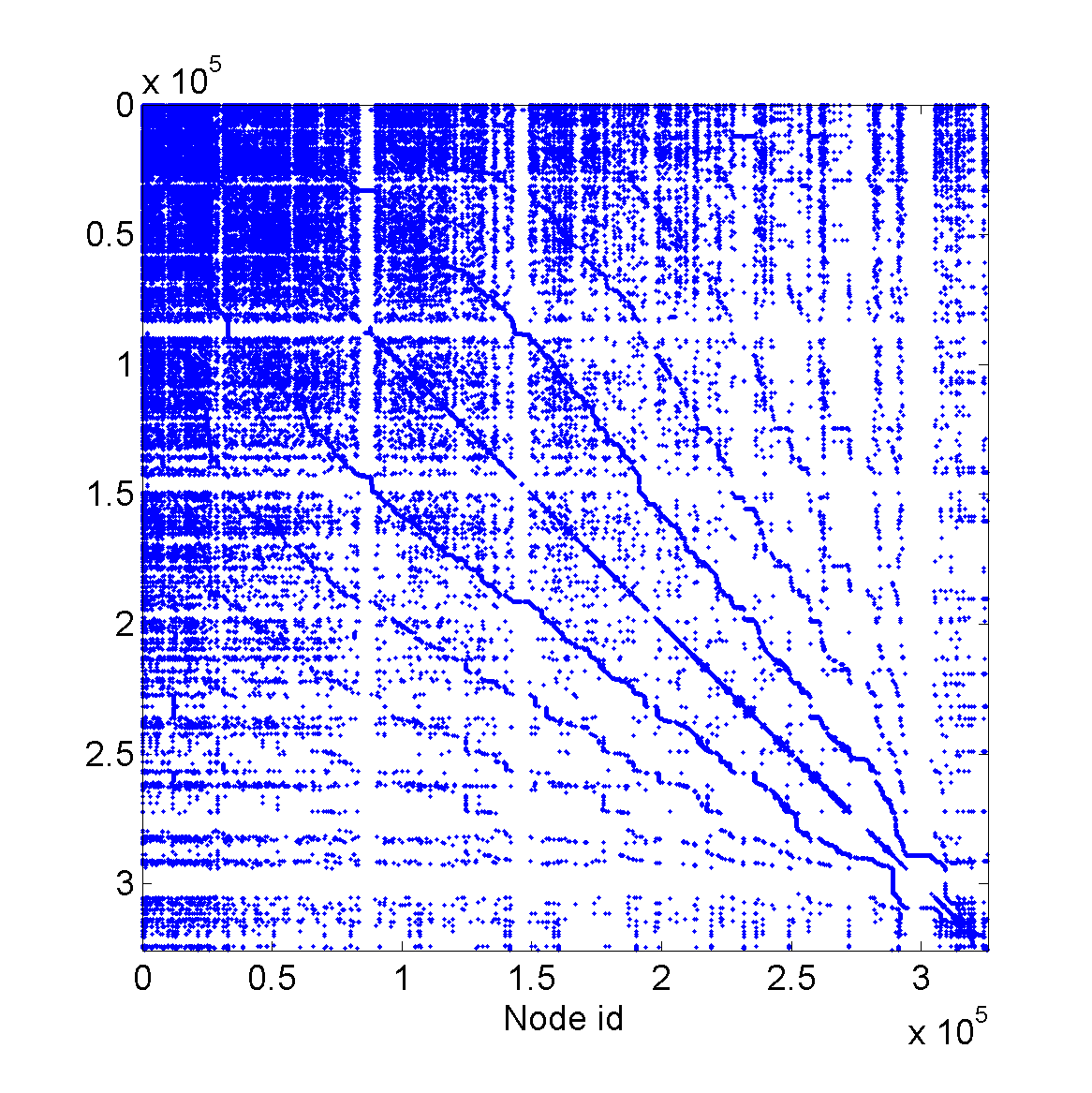
(l) www

Figure 11: Adjacency matrices for various real-world networks.

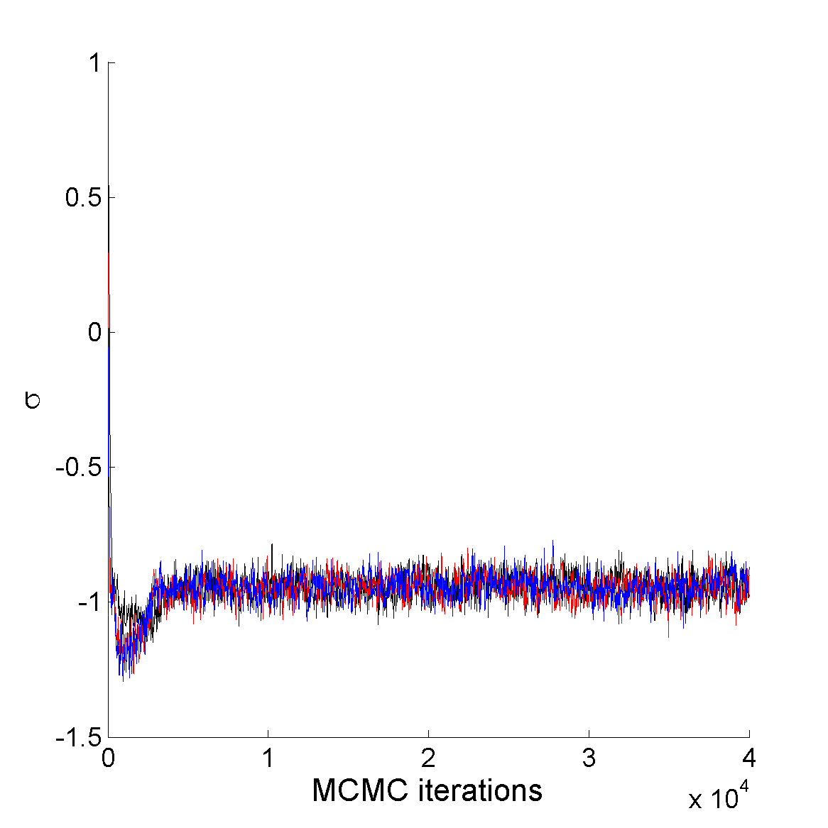
(a) facebook107

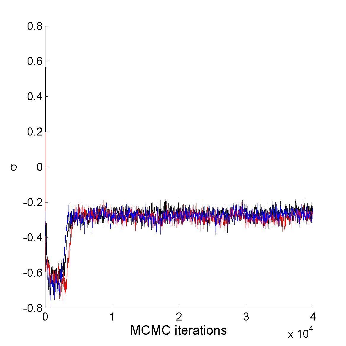
(b) polblogs

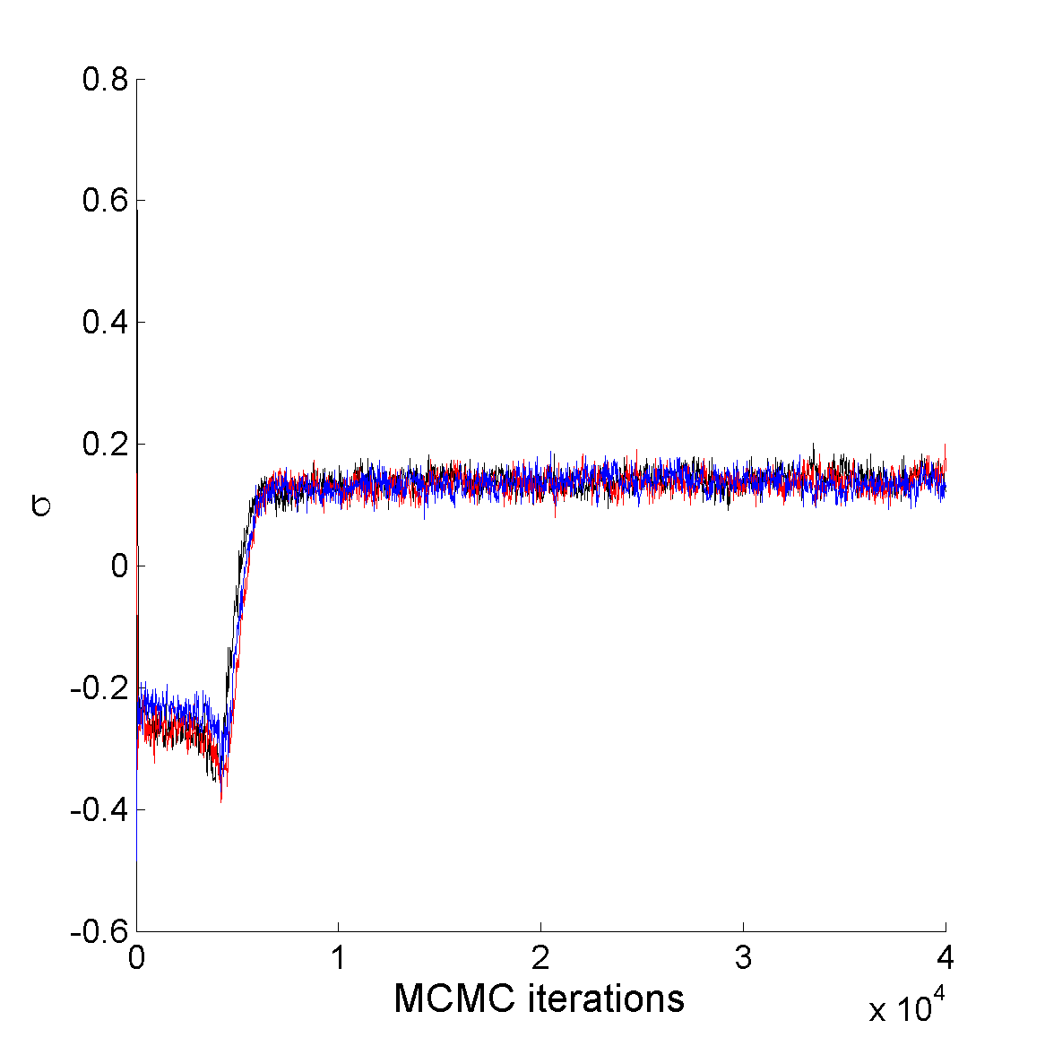
(c) USairport

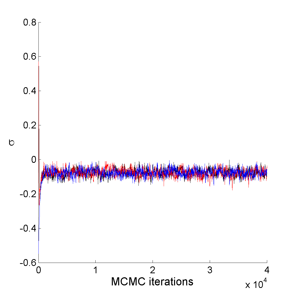
(d) UCirvine

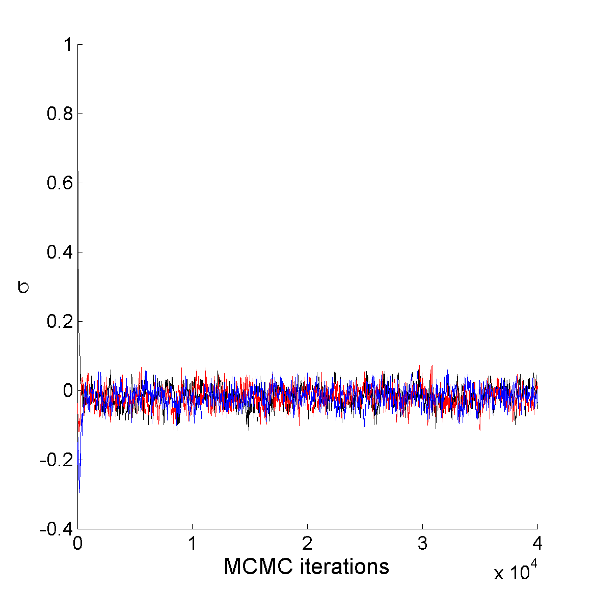
(e) yeast

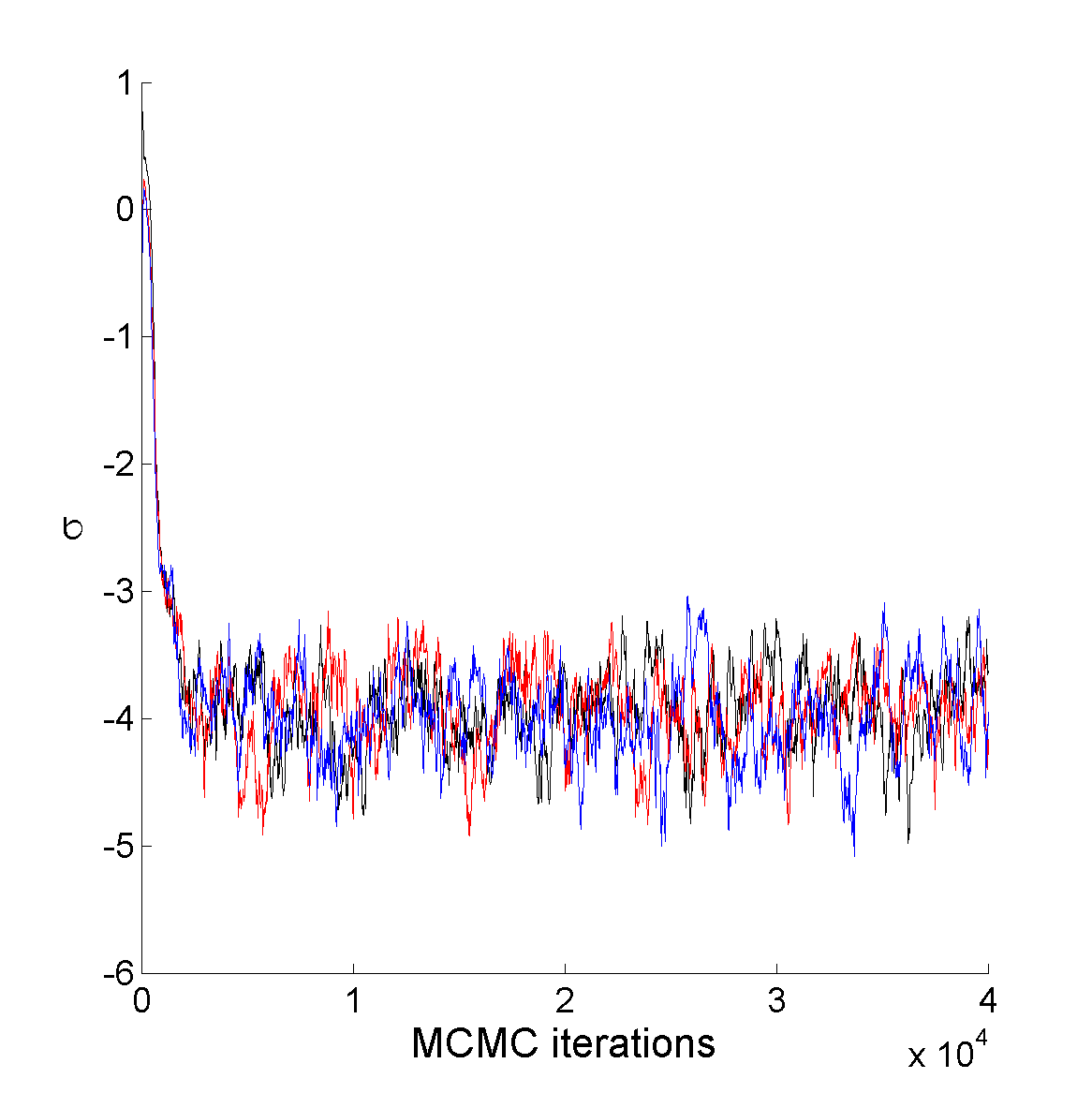
(f) USpower

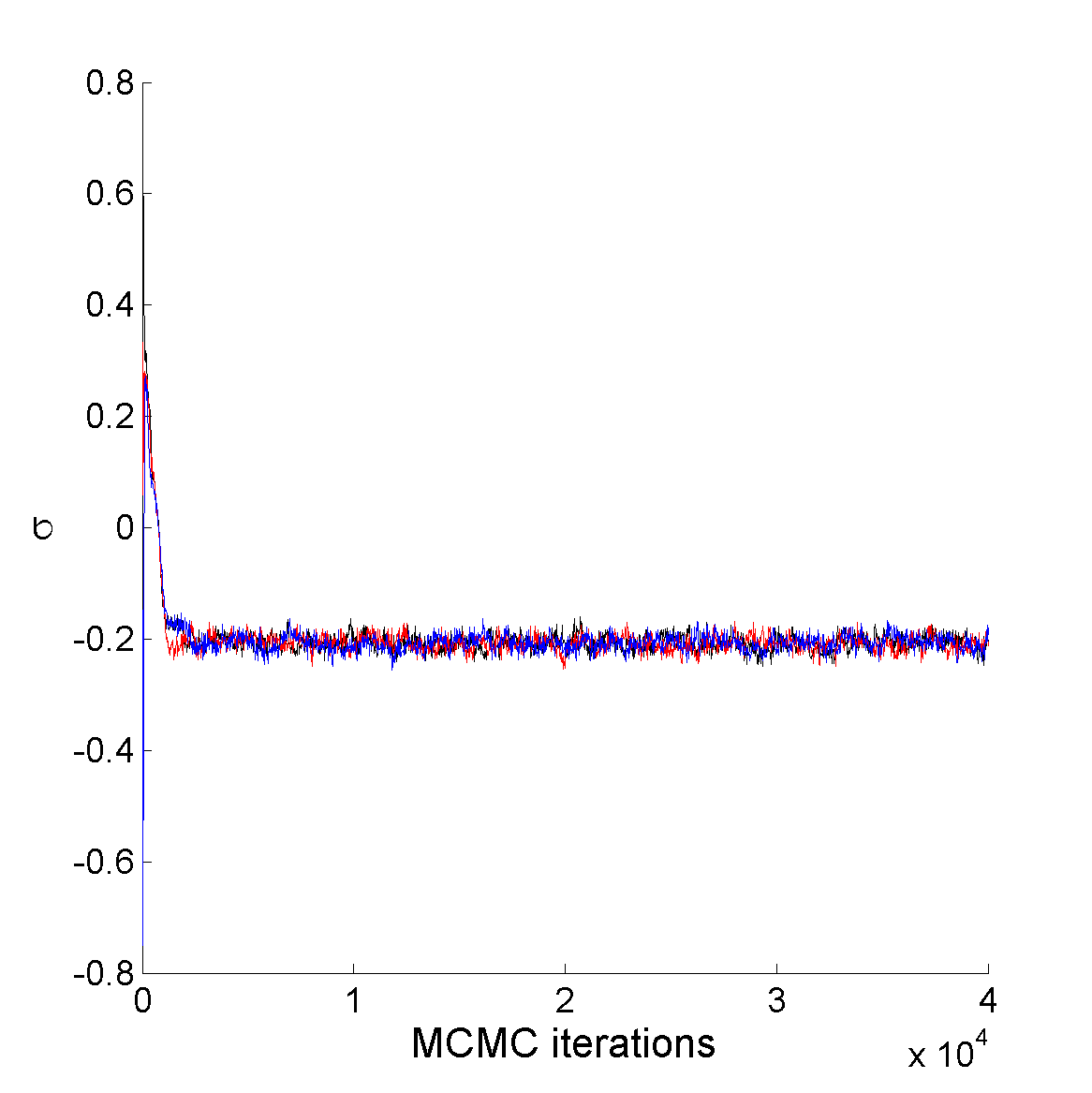
(g) IMDB

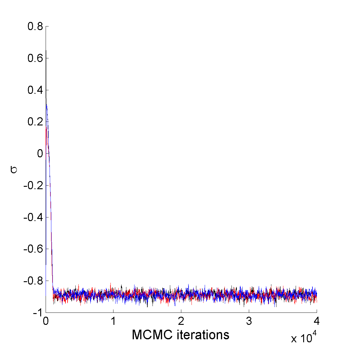
(h) cond-mat1

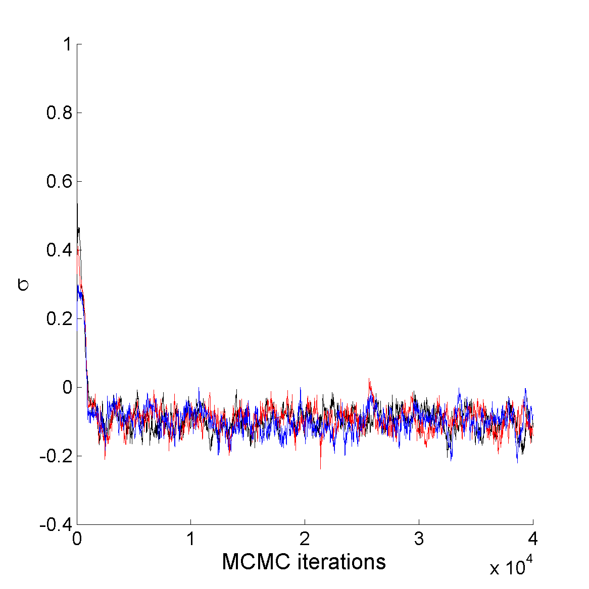
(i) cond-mat2

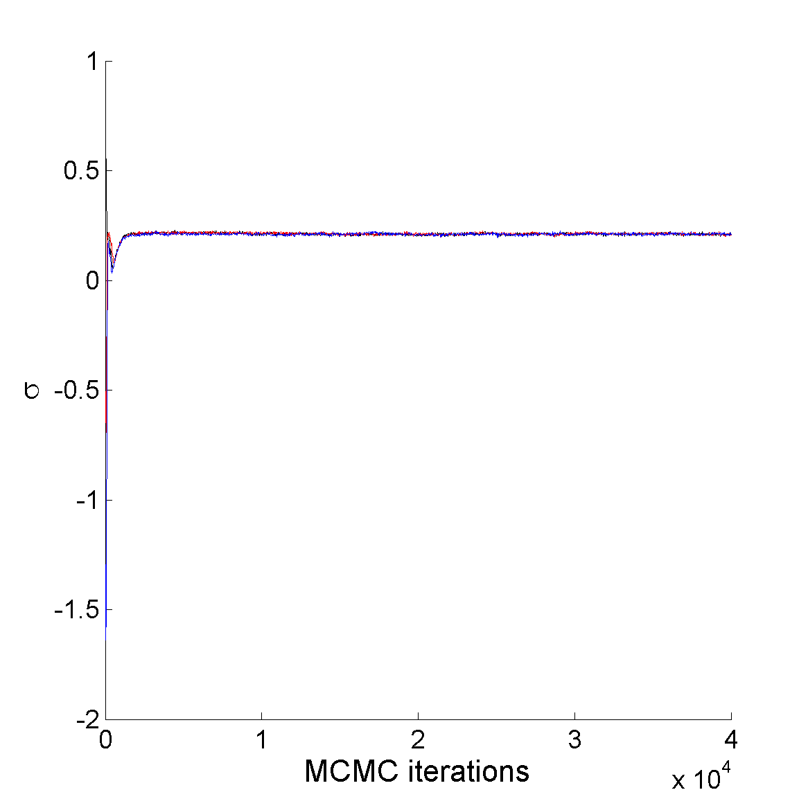
(j) enron

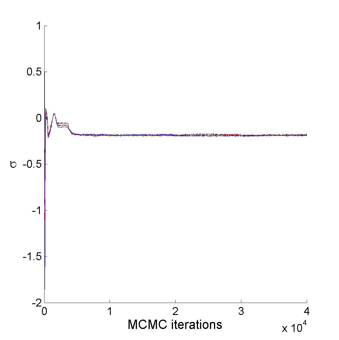
(k) internet

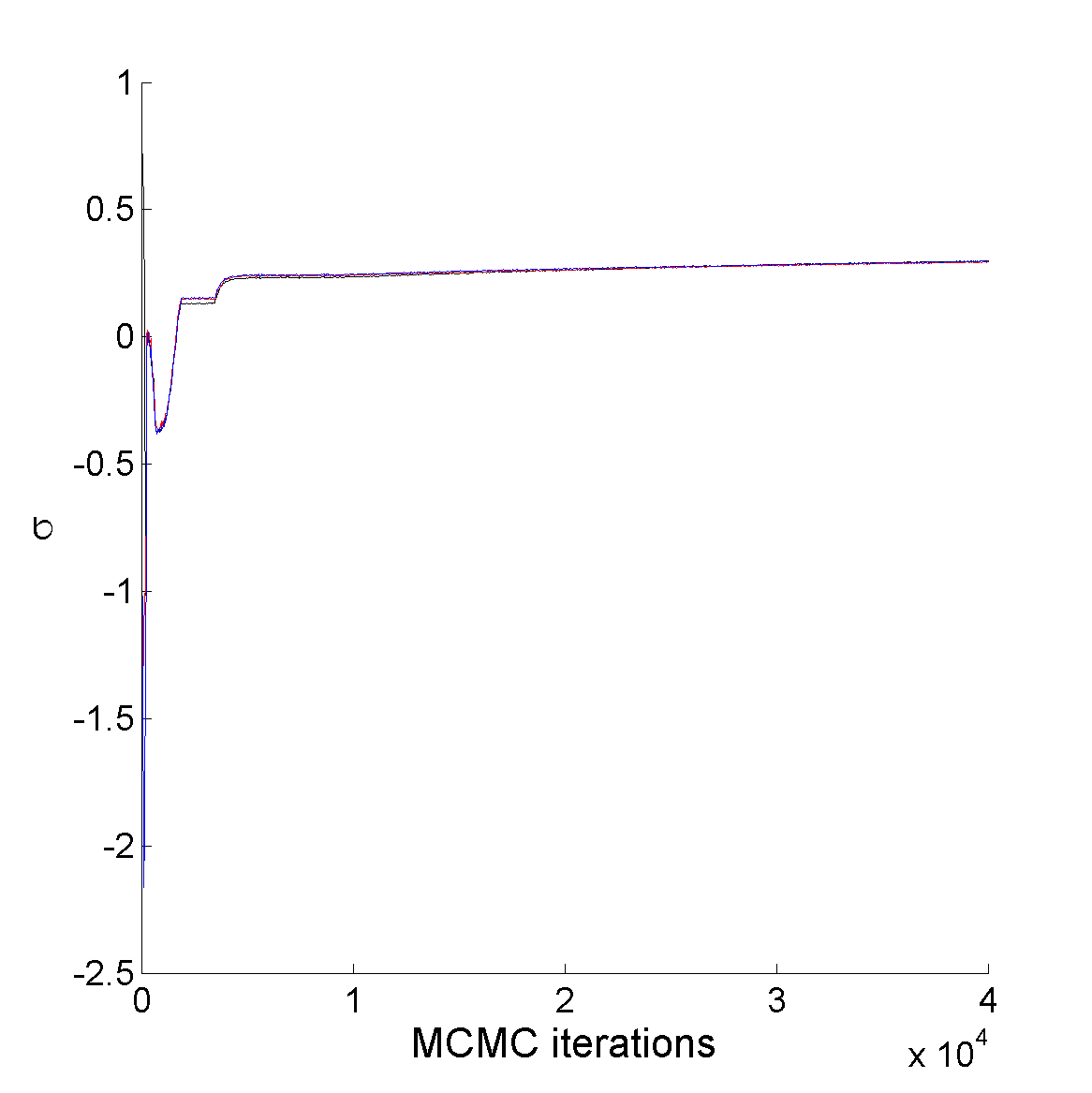
(l) www

Figure 12: MCMC trace plot for the parameter $\sigma$ for various real-world networks.

(a) facebook107

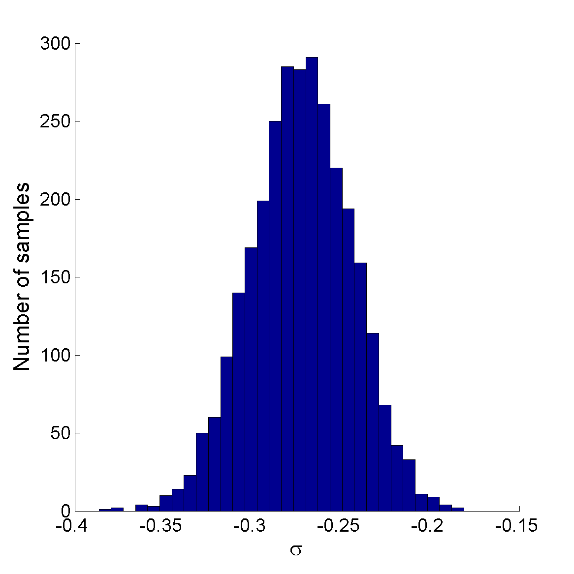
(b) polblogs

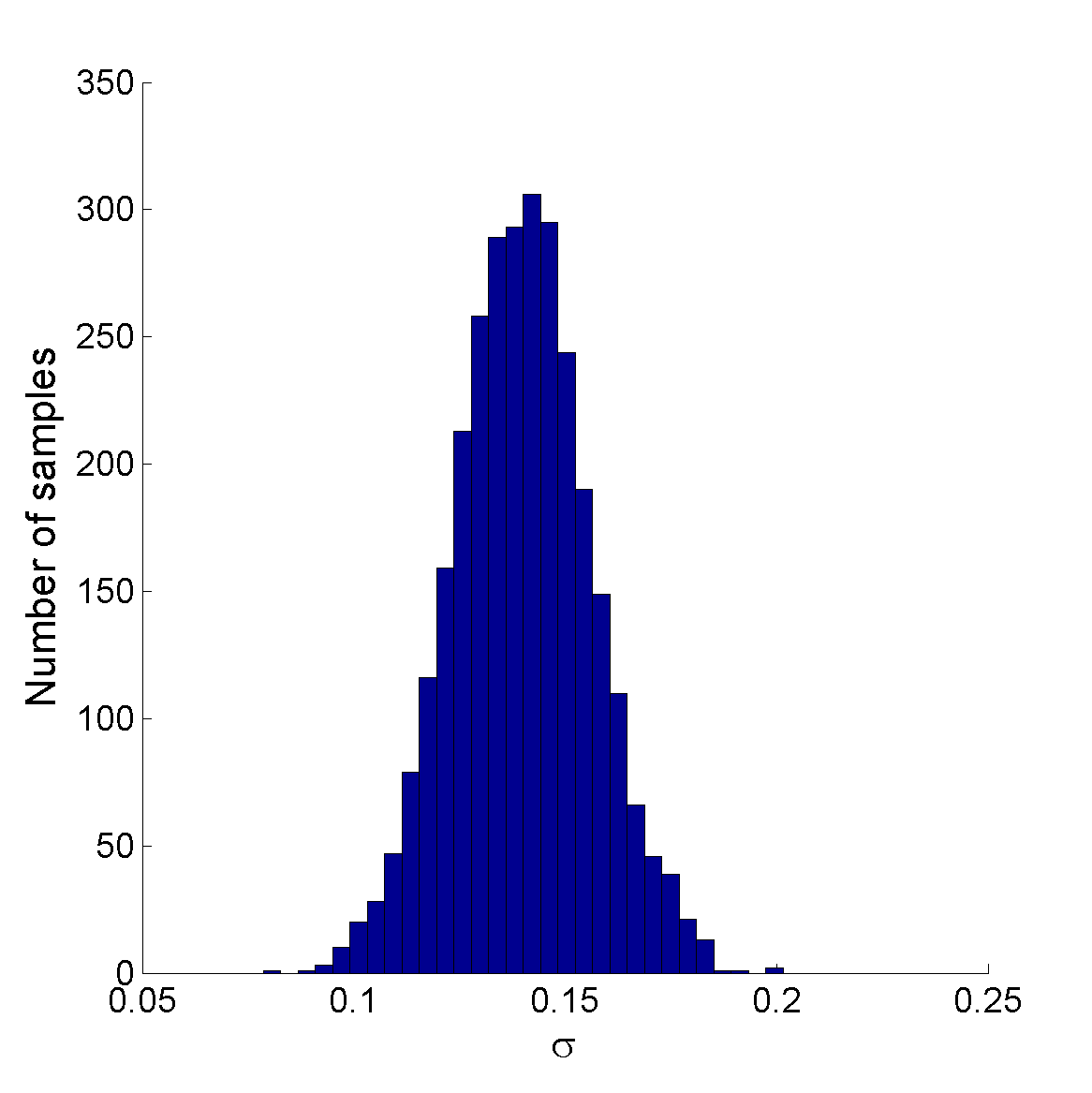
(c) USairport

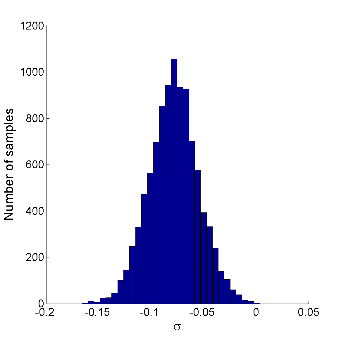
(d) UCirvine

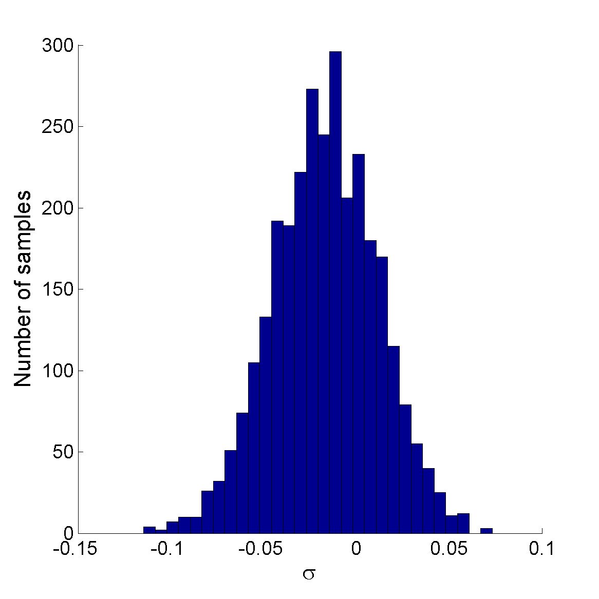
(e) yeast

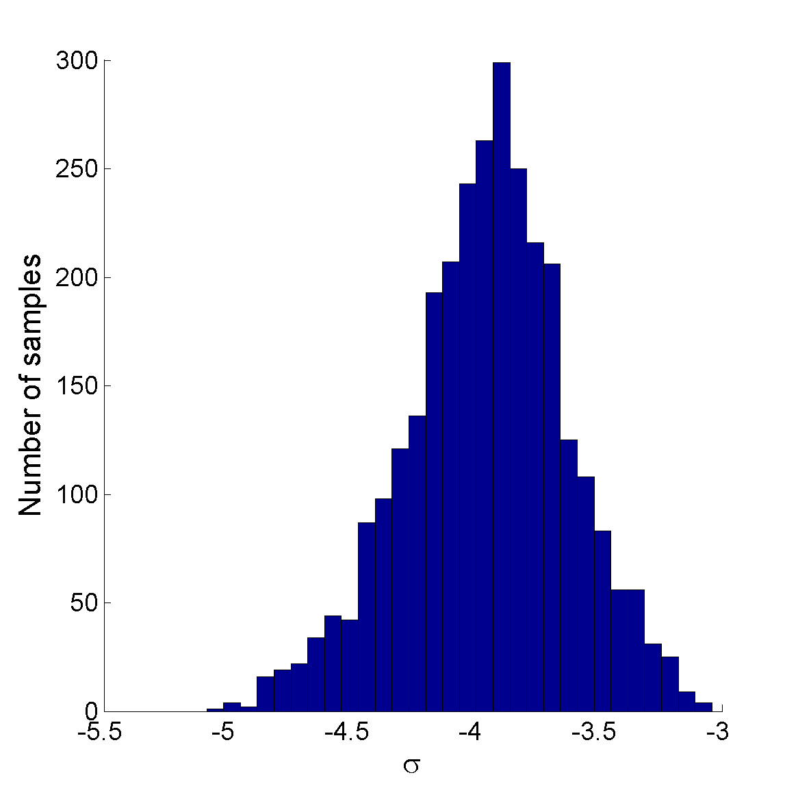
(f) USpower

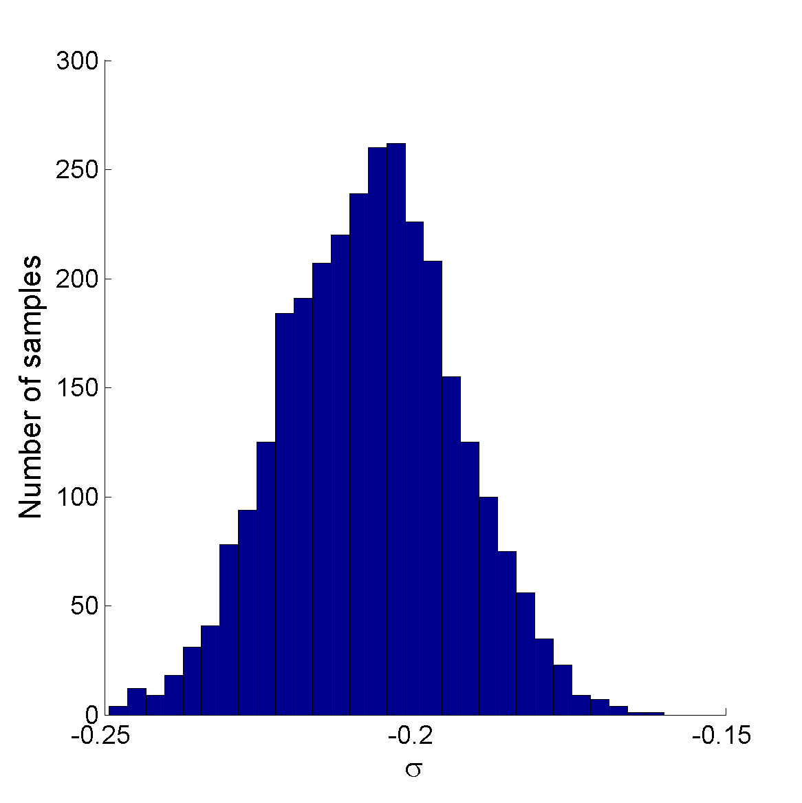
(g) IMDB

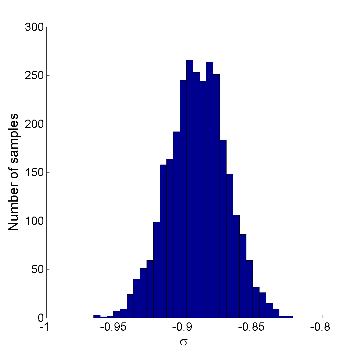
(h) cond-mat1

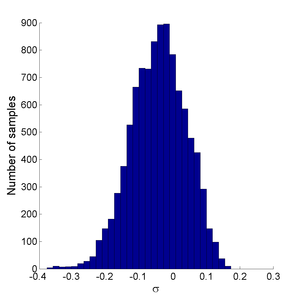
(i) cond-mat2

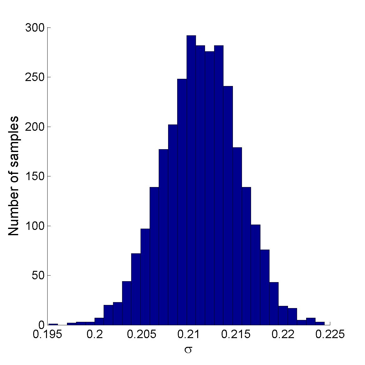
(j) enron

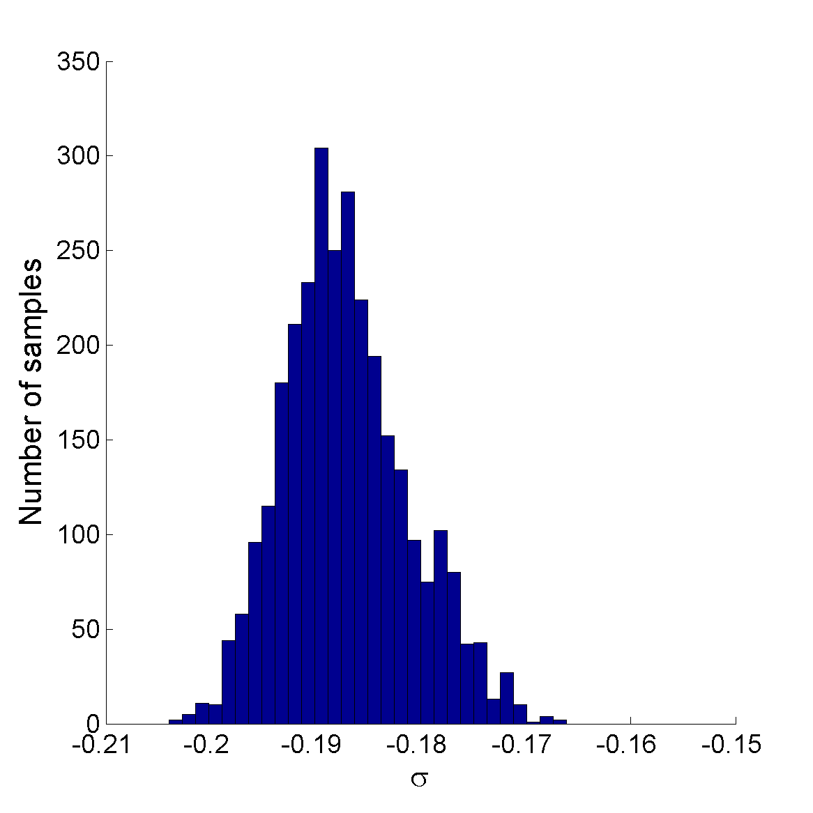
(k) internet

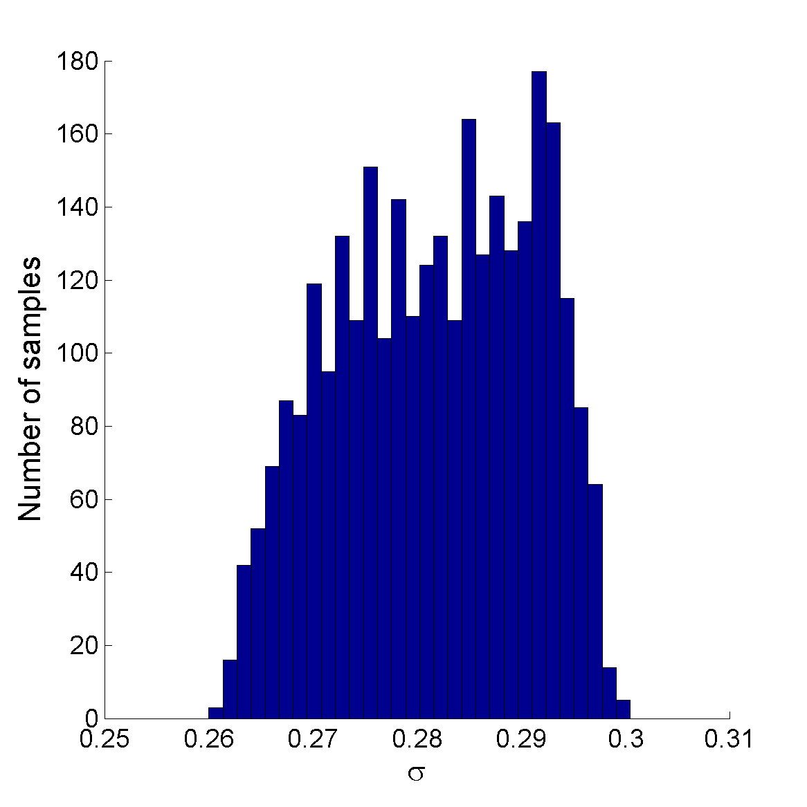
(l) www

Figure 13: Histograms of MCMC samples of the parameter $\sigma$ for various real-world networks.

(a) facebook107

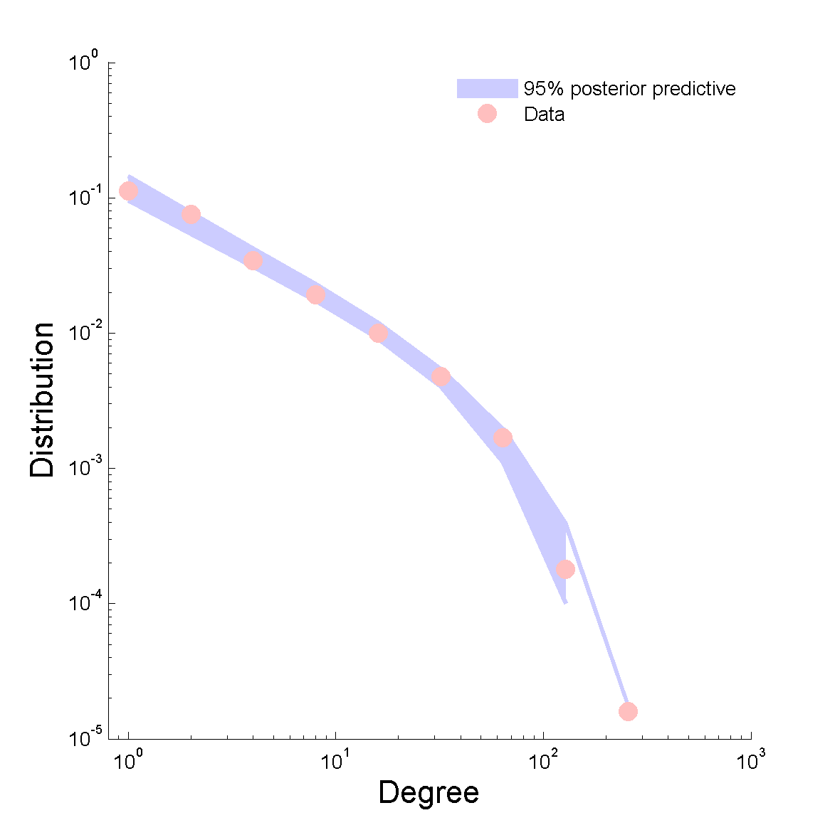
(b) polblogs

(c) USairport

(d) UCirvine

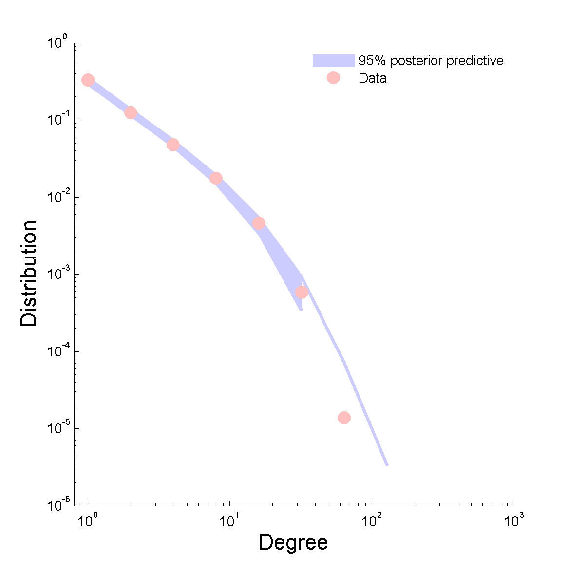
(e) yeast

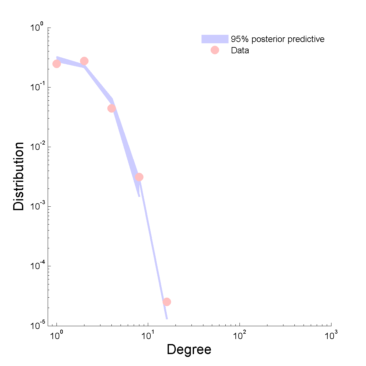
(f) USpower

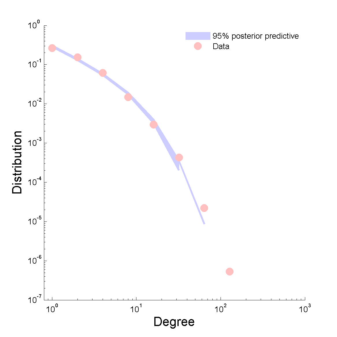
(g) IMDB

(h) cond-mat1

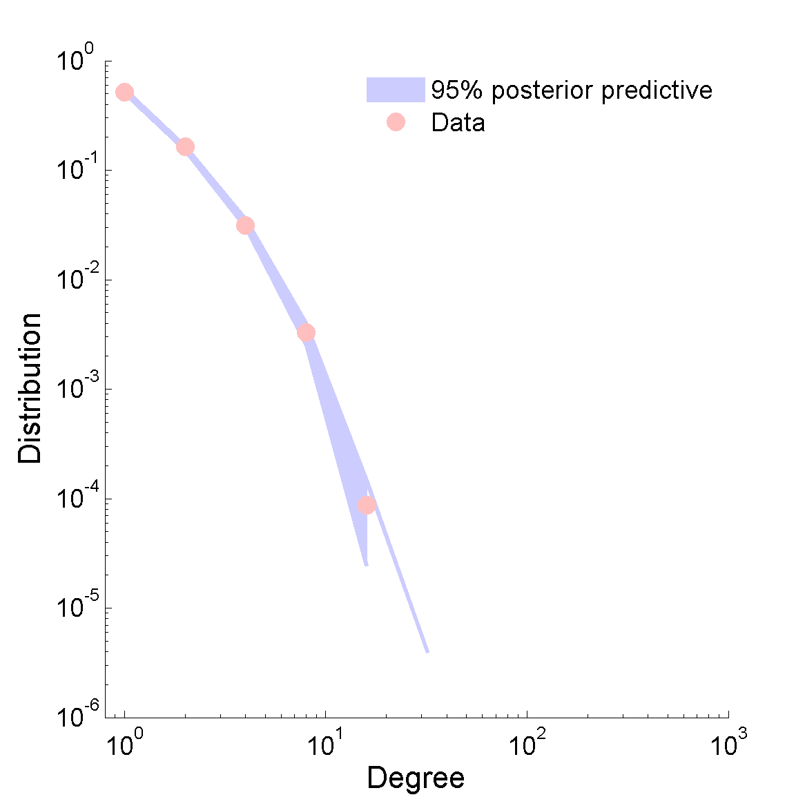
(i) cond-mat2

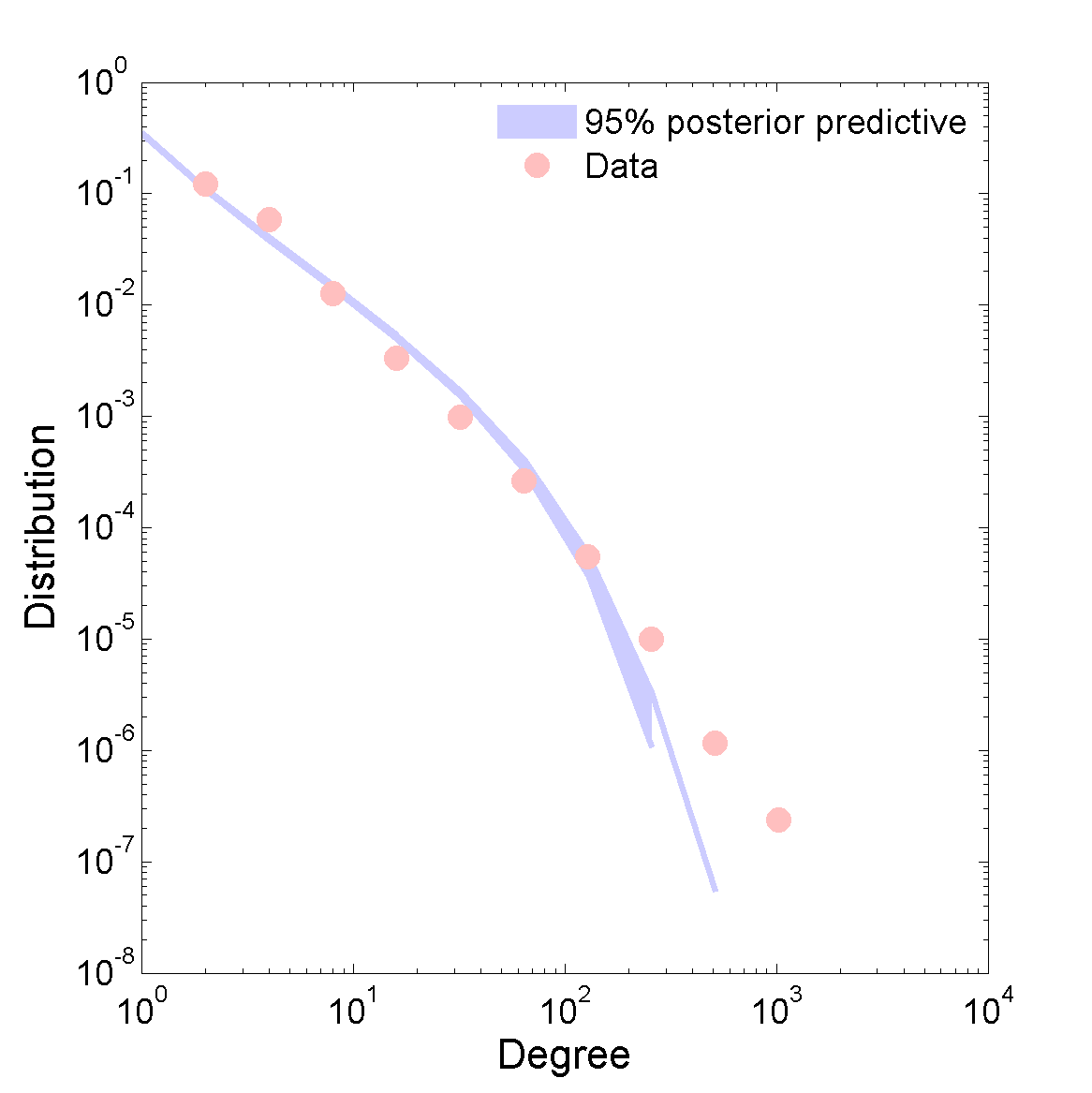
(j) enron

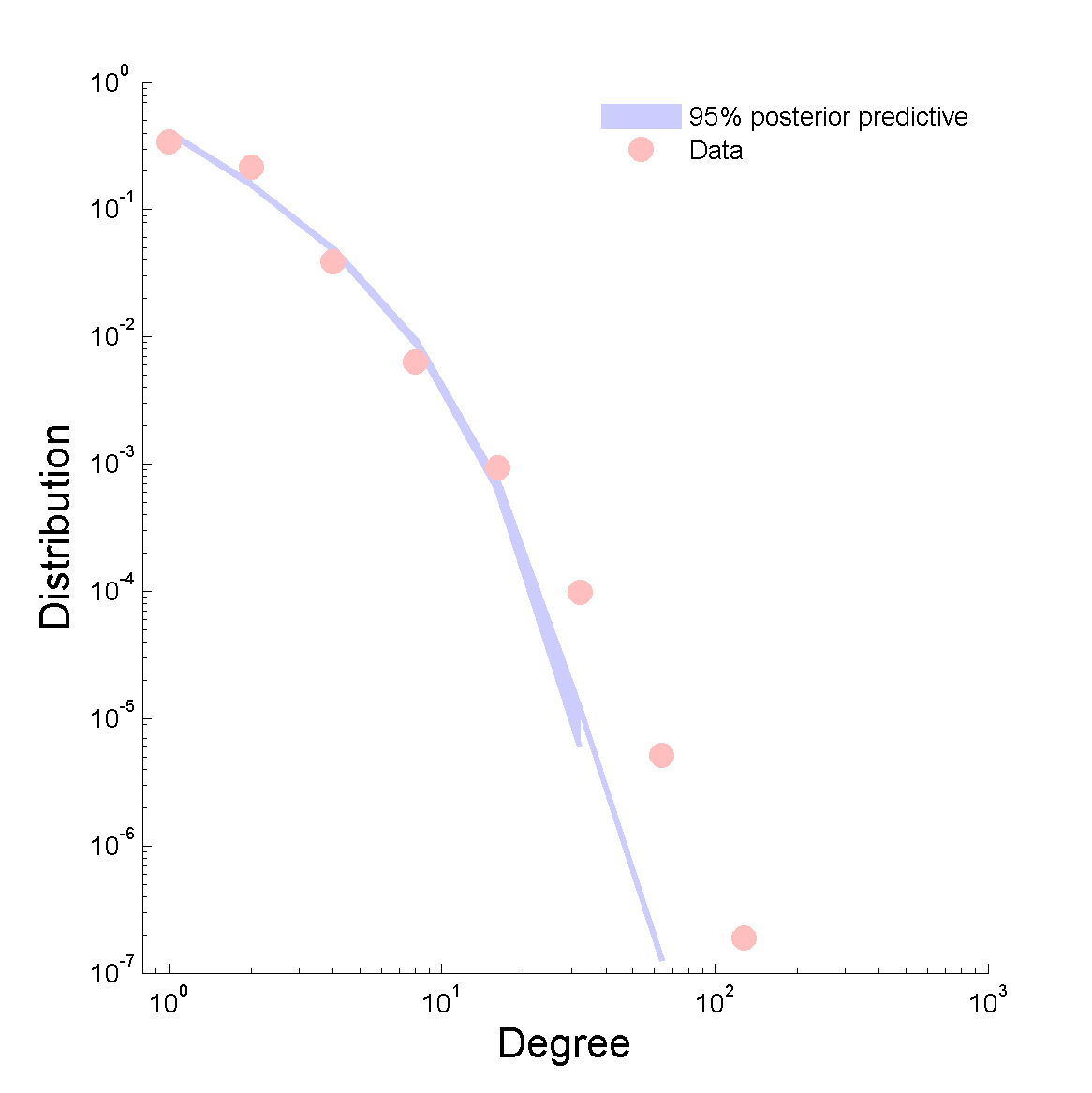
(k) internet

(l) www

Figure 14: Empirical degree distribution (red) and posterior predictive (blue) for various real-world networks.

8 Discussion

There has been extensive work over the past years on flexible Bayesian nonparametric models for networks, allowing complex latent structures of unknown dimension to be uncovered from real-world networks (Kemp et al., 2006; Miller, Griffiths and Jordan, 2009; Lloyd et al., 2012; Palla, Knowles and Ghahramani, 2012; Herlau, Schmidt and Mørup, 2014). However, as mentioned in the unifying overview of Orbanz and Roy (2015), these methods all fit in the Aldous-Hoover framework and as such produce dense graphs.

Norros and Reittu (2006) (see also (van der Hofstad, 2014) for a review and (Britton, Deijfen and Martin-Löf, 2006) for a similar model) proposed a conditionally Poissonian multigraph process with similarities to be drawn to our multigraph process. They consider that each node has a given sociability parameter, and the number of edges between two nodes $i$ and $j$ is drawn from a Poisson distribution with rate the product of the sociability parameters, normalized by the sum of the sociability parameters of all the nodes. The normalization makes this model similar to models based on rescaling of the graphon and, as such, does not define a projective model, as explained in Section 1.

Another related model is the degree-corrected random graph model (Karrer and Newman, 2011), where edges of the multigraph are drawn from a Poisson distribution whose rate is the product of node-specific sociability parameters and a parameter tuning the interaction between the latent communities to which these nodes belong. When the sociability parameters are assumed to be i.i.d. from some distribution, this model yields an exchangeable matrix and thus a dense graph.

Additionally, there are similarities to be drawn with the extensive literature on latent space modeling (cf. Hoff, Raftery and Handcock, 2002; Penrose, 2003; Hoff, 2009). In such models, nodes are embedded in a low-dimensional, continuous latent space and the probability of an edge is determined by a distance or similarity metric of the node-specific latent factors. In our case, the node position, $\theta_{i}$, is of no importance in forming edge probabilities. It would, however, be possible to extend our approach to location-dependent connections by considering inhomogenous CRMs.

Finally, the urn construction described in Section 3.2 highlights a connection with the configuration model (Bollobás, 1980; Newman, 2009), a popular model for generating simple graphs with a given degree sequence. The configuration model proceeds as follows. First, the degree $k_{i}$ of each node $i=1,\ldots,n$ is specified such that the sum of $k_{i}$ is an odd number. Each node $i$ is given a total of $k_{i}$ stubs, or demi-edges. Then, we repeatedly choose pairs of stubs uniformly at random, without replacement, and connect the selected pairs to form an edge. The simple graph is obtained either by discarding the multiple edges and self-loops (an erased configuration model), or by repeating the above sampling until obtaining a simple graph.

The connections to this past work nicely place our proposed Bayesian nonparametric network model within the context of existing literature. Importantly, however, to the best of our knowledge this work represents the first fully generative and projective approach to sparse graph modeling, and with a notion of exchangeability essential for devising our scalable statistical estimation procedure. For this, we devised a sampler that readily scales to large, real-world networks. The foundational modeling tools and theoretical results presented herein represent an important building block for future developments, including incorporating notions of community structure, node attributes, etc.

Acknowledgements.

The authors thank Bernard Bercu for help in deriving the proof of Theorem B.21, and Arnaud Doucet, Yee Whye Teh, Stefano Favaro and Dan Roy for helpful discussions and feedback on earlier versions of this paper.

Appendix A Proofs of results on the sparsity

A.1 Probability asymptotics notation

We first describe the asymptotic notation used in the remaining of this section, which follows the notation of Janson (2011). All unspecified limits are as $\alpha\rightarrow\infty$.

Let $(X_{\alpha})_{\alpha\geq 0}$ and $(Y_{\alpha})_{\alpha\geq 0}$ be two $[0,\infty)$-valued stochastic processes defined on the same probability space and such that $\lim_{\alpha\rightarrow\infty}X_{\alpha}=\lim_{\alpha\rightarrow\infty}Y_{\alpha}=\infty$ a.s. We have

$$X_{\alpha}=O(Y_{\alpha})\text{ a.s.} \Longleftrightarrow\underset{\alpha\rightarrow\infty}{\lim\sup}\ \frac{X_{\alpha}}{Y_{\alpha}}<\infty\text{ a.s.}$$

$$X_{\alpha}=o(Y_{\alpha})\text{ a.s.} \Longleftrightarrow\lim_{\alpha\rightarrow\infty}\frac{X_{\alpha}}{Y_{\alpha}}=0\text{ a.s.}$$

$$X_{\alpha}=\Omega(Y_{\alpha})\text{ a.s.} \Longleftrightarrow Y_{\alpha}=O(X_{\alpha})\text{ a.s.}$$

$$X_{\alpha}=\omega(Y_{\alpha})\text{ a.s.} \Longleftrightarrow Y_{\alpha}=o(X_{\alpha})\text{ a.s.}$$

$$X_{\alpha}=\Theta(Y_{\alpha})\text{ a.s.} \Longleftrightarrow X_{\alpha}=O(Y_{\alpha})\text{ and }X_{\alpha}=\Omega(Y_{\alpha})\text{ a.s.}$$

The relations have the following interpretation

$X_{\alpha}=O(Y_{\alpha})$	“$X_{\alpha}$ does not grow at a faster rate than $Y_{\alpha}$”	$[~{}\leq~{}]$
$X_{\alpha}=o(Y_{\alpha})$	“$X_{\alpha}$ grows at a (strictly) slower rate than $Y_{\alpha}$”	$[~{}<~{}]$
$X_{\alpha}=\Omega(Y_{\alpha})$	“$X_{\alpha}$ does not grow at a slower rate than $Y_{\alpha}$”	$[~{}\geq~{}]$
$X_{\alpha}=\omega(Y_{\alpha})$	“$X_{\alpha}$ grows at a (strictly) faster rate than $Y_{\alpha}$”	$[~{}>~{}]$
$X_{\alpha}=\Theta(Y_{\alpha})$	“$X_{\alpha}$ and $Y_{\alpha}$ grow at the same rate”	$[~{}=~{}]$

A.2 Proof of Theorems 4.6, 4.7 and 4.8 in the finite-activity case

We first consider the case of a finite-activity CRM. Let $T=\int_{0}^{\infty}\rho(w)dw<\infty$ and $H(t)=\frac{1}{T}\int_{0}^{t}\rho(w)dw$. The point process $Z$ can be equivalently defined as follows. Let $\Pi=\{\theta_{1},\theta_{2},\ldots\}$ be a homogeneous Poisson process of rate $T$. For each $1\leq i\leq j$, sample

$$z_{ij}|U_{i},U_{j}\sim\text{Ber}(W(U_{i},U_{j}))$$ (60)

where $U_{1},U_{2},\ldots$ are uniform random variables and

$$W(u,v)=\left\{\begin{array}[c]{ll}1-\exp(-2H^{-1}(u)H^{-1}(v))&u\neq v\\ 1-\exp(-H^{-1}(u)^{2})&u=v\end{array}\right.$$

Let $J_{\alpha}=\Pi\cap[0,\alpha].$ As (i) $J_{\alpha}\rightarrow\infty$ almost surely as $\alpha\rightarrow\infty$ and (ii) $\int_{0}^{1}\int_{0}^{1}W(u,v)dudv<\infty$ and $\int_{0}^{1}\sqrt{W(u,u)}du<\infty$, the law of large numbers for $V$ statistics yields (cf Theorem B.20)

$$\frac{2}{J_{\alpha}(J_{\alpha}+1)}\sum_{1\leq i\leq j\leq J_{\alpha}}W(U_{i},U_{j})\rightarrow\int_{0}^{1}\int_{0}^{1}W(u,v)dudv$$ (61)

almost surely as $\alpha\rightarrow\infty$. Additionally, applying Theorem B.21 to Equation (60), gives

$$\frac{N_{\alpha}^{(e)}}{\sum_{1\leq i\leq j\leq J_{\alpha}}W(U_{i},U_{j})}\rightarrow 1$$

a.s. which, combined with Equation (61) yields $\frac{N_{\alpha}^{(e)}}{J_{\alpha}^{2}}=\Theta(1)$ almost surely. As $\frac{N_{\alpha}}{J_{\alpha}}=\Theta(1)$ almost surely, we determine that

$$N_{\alpha}^{(e)} =\Theta(N_{\alpha}^{2})\text{ a.s.}$$

$$N_{\alpha} =\Theta(\alpha)\text{ a.s.}$$

$$N_{\alpha}^{(e)} =\Theta(\alpha^{2})\text{ a.s.}$$

A.3 Proof of Theorem 4.7 in the infinite-activity case

Consider now the infinite-activity case. Assume $\psi^{\prime}(0)=\mathbb{E}[W_{1}^{\ast}]<\infty.$ Let

$$\widetilde{Z}_{ij}=\left\{\begin{array}[c]{ll}1&\text{if }Z([i-1,i],[j-1,j])>0\\ 0&\text{otherwise}\end{array}\right.$$ (62)

then, for any $k\in\mathbb{N}$,

$$\sum_{1\leq i<j\leq k}\widetilde{Z}_{ij}\leq N_{k}^{(e)}\leq D_{k}^{\ast}$$ (63)

As $Z$ is a jointly exchangeable point process, $(\widetilde{Z}_{ij})_{i,j\in\mathbb{N}}$ is a jointly exchangeable binary matrix, and so by Theorem B.18,

$$\sum_{1\leq i<j\leq k}\widetilde{Z}_{ij}=\Theta(k^{2})$$ (64)

Moreover, we have

$$D_{k}^{\ast}|W_{k}\sim\text{Poisson}(W_{k}^{\ast 2})$$ (65)

where $W_{k}^{\ast}=\sum_{1\leq i\leq j\leq k}W([i-1,i])W([j-1,j])$, so Theorems B.21 and B.20 imply (as $\mathbb{E}[W_{1}^{\ast}]<\infty$)

$$D_{k}^{\ast}=\Theta(k^{2})$$ (66)

We therefore conclude that

$$N_{k}^{(e)}=\Theta(k^{2})$$ (67)

Finally, for any $k\leq\alpha\leq k+1$,

$$\frac{k^{2}}{(k+1)^{2}}\frac{N_{k}^{(e)}}{k^{2}}\leq\frac{N_{\alpha}^{(e)}}{\alpha^{2}}\leq\frac{(k+1)^{2}}{k^{2}}\frac{N_{k+1}^{(e)}}{(k+1)^{2}}$$

and as $\frac{k+1}{k}\rightarrow 1$ we conclude

$$N_{\alpha}^{(e)}=\Theta(\alpha^{2})\text{ a.s. as }\alpha\rightarrow\infty$$ (68)

A.4 Proof of Theorem 4.8 in the infinite-activity case

Consider sets $\mathcal{S}^{1}=\cup_{k\in\mathbb{N}}[\frac{2k+1}{2},\frac{2k+2}{2})$ and $\mathcal{S}^{2}=\cup_{k\in\mathbb{N}}[\frac{2k}{2},\frac{2k+1}{2})$. $\mathcal{S}^{1}$ and $\mathcal{S}^{2}$ define a partition of $\mathbb{R}_{\mathbb{+}}$ as $\mathcal{S}^{1}\cup\mathcal{S}^{2}=\mathbb{R}_{\mathbb{+}}$ and $\mathcal{S}^{1}\cap\mathcal{S}^{2}=\emptyset$. Let $\mathcal{S}_{\alpha}^{1}=\mathcal{S}^{1}\cap[0,\alpha]$ and $\mathcal{S}_{\alpha}^{2}=\mathcal{S}^{2}\cap[0,\alpha]$. Note that for $\alpha$ integer, $\lambda(\mathcal{S}_{\alpha}^{1})=\lambda(\mathcal{S}_{\alpha}^{2})=\frac{\alpha}{2}$.

Let $\widetilde{N}_{\alpha}$ be the number of nodes $\theta_{i}\in\mathcal{S}_{\alpha}^{1}$ with at least one directed edge to a node $\theta_{j}\in\mathcal{S}_{\alpha}^{2}$. Hence

$$\widetilde{N}_{\alpha}=\#\left\{\left.\theta_{i}\in\mathcal{S}_{\alpha}^{1}\ \right|\ D\left(\{\theta_{i}\}\times\mathcal{S}_{\alpha}^{2}\right)>0\right\}$$

Clearly, for all $\alpha\geq 0$

$$\widetilde{N}_{\alpha}\leq N_{\alpha}$$ (69)

We have, for $\theta_{i}\in\mathcal{S}_{\alpha}^{1}$

$$\Pr\left(\left.D\left(\{\theta_{i}\}\times\mathcal{S}_{\alpha}^{2}\right)>0\right|W\right)=1-\exp\left[-W(\{\theta_{i}\})\times W\left(\mathcal{S}_{\alpha}^{2}\right)\right]$$

Note the key fact that $W(\{\theta_{i}\})$ is independent of $W\left(\mathcal{S}_{\alpha}^{2}\right)$ as $\theta_{i}\notin\mathcal{S}_{\alpha}^{2}$. Applying Campbell’s theorem, we have

$$\mathbb{E}\left[\widetilde{N}_{\alpha}|W\left(\mathcal{S}_{\alpha}^{2}\right)\right]=\lambda(\mathcal{S}_{\alpha}^{1})\times\psi(W\left(\mathcal{S}_{\alpha}^{2}\right))$$

where $\psi(t)=\int_{0}^{\infty}(1-\exp(-wt))\rho(w)dw$ is the Laplace exponent. And so, by complete randomness of the CRM over $S_{n}^{1}$,

$$\widetilde{N}_{\alpha}|W\left(\mathcal{S}_{\alpha}^{2}\right)\sim\text{Poisson}\left(\lambda(\mathcal{S}_{\alpha}^{1})\times\psi(W\left(\mathcal{S}_{\alpha}^{2}\right))\right)$$ (70)

We have $\lambda(\mathcal{S}_{\alpha}^{1})=\Theta(\alpha)$ and $\lambda(\mathcal{S}_{\alpha}^{2})=\Theta(\alpha)$. Moreover, as we are in the infinite-activity case $\int_{0}^{\infty}\rho(w)dw=\infty$, Lemma B.25 implies that

$$\lim_{t\rightarrow\infty}\psi(t)=\infty.$$ (71)

As $W\left(\mathcal{S}_{\alpha}^{2}\right)\rightarrow\infty$ almost surely, we therefore have $\psi(W\left(\mathcal{S}_{\alpha}^{2}\right))\rightarrow\infty$ almost surely. Thus,

$$\psi(W\left(\mathcal{S}_{\alpha}^{2}\right))=\omega(1)\text{ a.s.}$$ (72)

and

$$\lambda(\mathcal{S}_{\alpha}^{1})\times\psi(W\left(\mathcal{S}_{\alpha}^{2}\right))=\omega(\alpha)\text{ a.s.}$$ (73)

Combining (73) with Theorem B.23 and (69) yields

$$\widetilde{N}_{\alpha} =\omega(\alpha)\text{ a.s.}$$ (74)

$$N_{\alpha} =\omega(\alpha)\text{ a.s.}$$ (75)

Consider now the case where $\overline{\rho}(x)\overset{x\downarrow 0}{\sim}\ell(1/x)x^{-\sigma}$ where $\ell(t)$ is a slowly varying function, i.e. a function verifying $\frac{\ell(ct)}{\ell(t)}\rightarrow 1$ for any $c>0$, and such that $\lim_{t\rightarrow\infty}\ell(t)>0.$ Then Lemma B.27 implies that $\psi(t)=\Omega(t^{\sigma})$ as $t\rightarrow\infty$ and thus

$$\lambda(\mathcal{S}_{\alpha}^{1})\times\psi(W\left(\mathcal{S}_{\alpha}^{2}\right))=\Omega(\alpha^{\sigma+1})\text{ a.s.}$$

which implies that

$$N_{\alpha}=\Omega(\alpha^{\sigma+1})\text{ a.s.}$$

Appendix B Technical lemmas

Theorem B.18 (Graphs constructed from exchangeable arrays are dense).

Let $(X_{ij})_{i,j\in\mathbb{N}},$ be an infinitely exchangeable binary symmetric array. Let $N_{n}=\sum_{1\leq i<j\leq n}X_{ij}$. If $\lim_{n\rightarrow\infty}N_{n}>0$ almost surely, then

$$N_{n}=\Theta(n^{2})\text{ almost surely and in }L_{1}$$ (76)

Proof B.19.

From the Aldous-Hoover theorem, there is a random function $W:[0,1]\rightarrow[0,1]$ such that

$$X_{ij}|W,U_{i},U_{j}\sim\operatorname{Ber}(W(U_{i},U_{j}))$$ (77)

where $(U_{i})_{i\in\mathbb{N}}$ are uniform random variables. Given $W$, the law of large numbers for $U$ statistics (see Theorem B.20) yields

$$\frac{2}{n(n-1)}\sum_{1\leq i<j\leq n}W(U_{i},U_{j})\rightarrow\overline{W}\text{ a.s.}$$

If $\lim_{n\rightarrow\infty}N_{n}>0$ almost surely, then $\overline{W}=\int_{0}^{1}\int_{0}^{1}W(u,v)dudv>0$ almost surely, thus

$$\sum_{1\leq i<j\leq n}W(U_{i},U_{j})=\Theta(n^{2})\text{ a.s.}$$ (78)

Furthermore, note that if $X|Y\sim\operatorname{Ber}(Y)$, $\mathbb{V}(X|Y)=Y(1-Y)\leq\mathbb{E}[X|Y\}$. Moreover, $\sum_{1\leq i<j\leq n}W(U_{i},U_{j})\rightarrow\infty$ almost surely. Applying Theorem B.21 to Eq. (77) implies

$$\frac{\sum_{1\leq i<j\leq n}X_{ij}}{\sum_{1\leq i<j\leq n}W(U_{i},U_{j})}\rightarrow 1\text{ a.s. as }n\rightarrow\infty$$ (79)

and thus, combining (78) with (79) yields

$$N_{n}=\Theta(n^{2})\text{ a.s. as }n\rightarrow\infty$$ (80)

As $X_{ij}\leq 1$, the dominated convergence theorem implies $\mathbb{E}[N_{n}]=\Theta(n^{2})$.

Lemma B.20 (Strong law of large numbers for U and V statistics).

(Arcones and Giné, 1992; Giné and Zinn, 1992). Let $(X_{i})$ be i.i.d. real-valued random variables from $\mu$ and let $h(x_{1},x_{2})$ be a symmetric measurable function. Consider the $U$ and $V$ statistics defined by

$$U_{n}(h,\mu) =\frac{2}{n(n-1)}\sum_{1\leq i<j\leq n}h(X_{i},X_{j})$$

$$V_{n}(h,\mu) =\frac{1}{n^{2}}\sum_{i,j=1}^{n}h(X_{i},X_{j})$$

If $\mathbb{E}[\left|h(X_{1},X_{2})\right|]<\infty$, then (Hoeffding, 1961)

$$U_{n}(h,\mu)\rightarrow\mathbb{E}[h(X_{1},X_{2})]\text{ a.s. as }n\rightarrow\infty$$

If $\mathbb{E}[\left|h(X_{1},X_{2})\right|]<\infty$ and $\mathbb{E}[\sqrt{\left|h(X_{1},X_{1})\right|}]<\infty$, then

$$V_{n}(h,\mu)\rightarrow\mathbb{E}[h(X_{1},X_{2})]\text{ a.s. as }n\rightarrow\infty.$$

Theorem B.21.

Let $Y=(Y_{1},Y_{2},\ldots)$ be a sequence of positive random variables. Consider positive variables $(X_{1},X_{2},\ldots)$ such that

$$\mathbb{E}[X_{i}|X_{1:i-1},Y_{1:i}] =\mathbb{E}[X_{i}|Y_{i}]=Y_{i}$$ (81)

$$\mathbb{V}[X_{i}|X_{1:i-1},Y_{1:i}] =\mathbb{V}[X_{i}|Y_{i}]\leq Y_{i}$$ (82)

If

$$\sum_{i=1}^{n}Y_{i}\rightarrow\infty\text{ almost surely as }n\rightarrow\infty$$

then

$$\frac{\sum_{i=1}^{n}X_{i}}{\sum_{i=1}^{n}Y_{i}}\rightarrow 1\text{ almost surely as }n\rightarrow\infty$$

Proof B.22.

We will use a martingale approach here. Note that it is also possible to use an alternative proof via Borel-Cantelli. Let $\mathbb{F}=(\mathcal{F}_{1},\mathcal{F}_{2},\ldots)$ be a filtration with $\mathcal{F}_{n}=\sigma(X_{1},\ldots,X_{n},Y_{1},\ldots,Y_{n+1})$. We have

$$\mathbb{E}[X_{n+1}|\mathcal{F}_{n}]=Y_{n+1}$$

Let $(M_{n})$ be defined as

$$M_{n}=\sum_{i=1}^{n}\frac{X_{i}-Y_{i}}{1+S_{i}}$$

where

$$S_{n}=\sum_{i=1}^{n}Y_{i}$$

$(M_{n})$ is a martingale with respect to the filtration $\mathbb{F}$ as $M_{n}$ is $\mathcal{F}_{n}$-measurable,

$$\mathbb{E}[M_{n+1}|\mathcal{F}_{n}] =M_{n}+\frac{1}{1+S_{n}}\left(\mathbb{E}[X_{n+1}|\mathcal{F}_{n}]-Y_{n+1}\right)$$

$$=M_{n}$$

and, using Hölder inequalities together with properties (81) and (82)

$$\mathbb{E}[M_{n}^{2}] \leq\sum_{i=1}^{n}\mathbb{E}\left[\frac{\left(X_{i}-Y_{i}\right)^{2}}{(1+S_{i})^{2}}\right]$$

$$\leq\sum_{i=1}^{n}\mathbb{E}\left[\frac{\left(X_{i}-Y_{i}\right)^{2}}{(1+Y_{i})^{2}}\right]$$

$$=\sum_{i=1}^{n}\mathbb{E}\left[\mathbb{E}\left[\left.\frac{\left(X_{i}-Y_{i}\right)^{2}}{(1+Y_{i})^{2}}\right|Y_{i}\right]\right]$$

$$=\sum_{i=1}^{n}\mathbb{E}\left[\frac{\mathbb{V}(X_{i}|Y_{i})}{(1+Y_{i})^{2}}\right]$$

$$\leq\sum_{i=1}^{n}\mathbb{E}\left[\frac{Y_{i}}{(1+Y_{i})^{2}}\right]$$

$$\leq n<\infty$$

Let

$$\mathbb{E}[(M_{n+1}-M_{n})^{2}|\mathcal{F}_{n}] =\frac{1}{(1+S_{n+1})^{2}}\mathbb{E}[(X_{n+1}-Y_{n+1})^{2}|\mathcal{F}_{n}]$$

$$=\frac{1}{(1+S_{n+1})^{2}}\mathbb{V}[X_{n+1}|\mathcal{F}_{n}]\leq\frac{Y_{n+1}}{(1+S_{n+1})^{2}}$$

It follows that

$$\left\langle M\right\rangle_{n} =\sum_{i=1}^{n}\mathbb{E}[(M_{i}-M_{i-1})^{2}|\mathcal{F}_{i-1}]$$

$$\leq\sum_{i=1}^{n}\frac{Y_{i}}{(1+S_{i})^{2}}$$

By Rieman integration,

$$\sum_{i=1}^{n}\frac{Y_{i}}{(1+\sum_{j=1}^{n}Y_{j})^{2}}\leq\int_{0}^{n}\frac{1}{(1+x)^{2}}dx<\infty$$

Therefore

$$\left\langle M\right\rangle_{\infty}=\lim_{n\rightarrow\infty}\left\langle M\right\rangle_{n}<\infty\text{ almost surely}$$

The law of large numbers for square-integrable martingales (see e..g. Theorem 5.4.9 page 217 of (Durrett, 2010)) thus implies that

$$\lim_{n\rightarrow\infty}M_{n}\text{ exists and is a.s. finite}$$

therefore

$$\sum_{i=1}^{n}\frac{X_{i}-Y_{i}}{1+S_{i}}<\infty\text{ a.s.}$$

As $1+S_{i}\rightarrow\infty$ almost surely, the lemma of Kronecker (Theorem 2.5.5. in (Durrett, 2010)) implies

$$\frac{1}{1+S_{n}}\sum_{i=1}^{n}\left(X_{i}-Y_{i}\right)\rightarrow 0\text{ a.s.}$$

and thus

$$\frac{\sum_{i=1}^{n}X_{i}}{\sum_{j=1}^{n}Y_{j}}\rightarrow 1\text{ a.s.}$$

Theorem B.23.

Let $\mu$ be a random almost surely positive measure on $\mathbb{R}_{+}$ and define the random integer valued measure $N$ as

$$N|\mu\sim\operatorname{Poisson}(\mu)$$

Write $\overline{N}_{t}=N([0,t])$ and $\overline{\mu}_{t}=\mu([0,t])$. Then

$$\overline{N}_{t}|\mu\sim\operatorname{Poisson}(\overline{\mu}_{t})$$

If $\overline{\mu}_{t}\rightarrow\infty$ almost surely and $\frac{\overline{\mu}_{t+1}}{\overline{\mu}_{t}}\rightarrow 1$ almost surely, then

$$\frac{\overline{N}_{t}}{\overline{\mu}_{t}}\rightarrow 1\text{ a.s.}$$

Proof B.24.

Let $k=1,2,\ldots.$, let $X_{k}=\overline{N}_{k}-\overline{N}_{k-1}$ and $Y_{k}=\overline{\mu}_{k}-\overline{\mu}_{k-1}$. From Theorem B.21, we have

$$\frac{\sum_{k=1}^{n}X_{k}}{\sum_{k=1}^{n}Y_{k}}\rightarrow 1\text{ as }n\rightarrow\infty$$

and so

$$\frac{\overline{N}_{n}}{\overline{\mu}_{n}}\rightarrow 1\text{ as }n\rightarrow\infty$$

As, for $n\leq t\leq n+1$

$$\frac{\overline{\mu}_{n}}{\overline{\mu}_{n+1}}\frac{\overline{N}_{n}}{\overline{\mu}_{n}}\leq\frac{\overline{N}_{t}}{\overline{\mu}_{t}}\leq\frac{\overline{N}_{n+1}}{\overline{\mu}_{n+1}}\frac{\overline{\mu}_{n+1}}{\overline{\mu}_{n}}$$

as $\frac{\overline{\mu}_{n+1}}{\overline{\mu}_{n}}\rightarrow 1$ almost surely, we conclude that

$$\frac{\overline{N}_{t}}{\overline{\mu}_{t}}\rightarrow 1\text{ a.s.}$$

Lemma B.25.

Let $Z_{t}$ be an almost surely increasing Lévy process (or subordinator) without deterministic component and with Lévy intensity $\rho(w)$. Let

$$\psi(t)=\int_{0}^{\infty}(1-\exp(-wt))\rho(w)dw$$

be its Laplace exponent. If

$$\int_{0}^{\infty}\rho(w)dw=\infty$$

then

$$\lim_{t\rightarrow\infty}\psi(t)=\infty.$$

Proof B.26.

Consider sequence of functions $f_{k}(w)=(1-\exp(-wk))\rho(w)$, $k\in\mathbb{N}.$ We have for

$$0\leq f_{k}(w)<f_{k+1}(w)\text{ for all }w>0$$

and

$$\lim_{k\rightarrow\infty}f_{k}(w)=\rho(w)$$

Thus, by Lebesgue’s monotone convergence theorem

$$\lim_{k\rightarrow\infty}\psi(k) =\int_{0}^{\infty}\rho(w)dw$$

$$=\infty$$

as $\psi(t)\geq\psi(\left\lfloor t\right\rfloor)$,

$$\lim_{t\rightarrow\infty}\psi(t)=\infty$$

Lemma B.27 (Relating tail Lévy intensity and Laplace exponent).

(Gnedin, Hansen and Pitman, 2007, Proposition 17) Let $\rho(w)$ be the Lévy intensity $\overline{\rho}(x)=\int_{x}^{\infty}\rho(w)dw$ be the tail Lévy intensity, and $\psi(t)=\int_{0}^{\infty}(1-\exp(-wt))\rho(w)dw$ its Laplace exponent. The following conditions are equivalent:

$$\overline{\rho}(x) \overset{x\downarrow 0}{\sim}\ell(1/x)x^{-\sigma}$$ (83)

$$\psi(t) \overset{t\uparrow\infty}{\sim}\Gamma(1-\sigma)t^{\sigma}\ell(t)$$ (84)

where $0<\sigma<1$ and $\ell$ is a function slowly varying at $\infty$ i.e. satisfying $\ell(cy)/\ell(y)\rightarrow 1$ as $y\rightarrow\infty$, for every $c>0$.

Proof B.28.

Applying integration by part, we have

$$\psi(t) =\int_{0}^{\infty}(1-\exp(-wt))\rho(w)dw$$

$$=t\int_{0}^{\infty}\exp(-wt)\overline{\rho}(w)dw$$

As $\overline{\rho}(x)$ is positive monotonic, application of Proposition B.29 yields the following equivalence

$$\overline{\rho}(x) \overset{x\downarrow 0}{\sim}\ell(1/x)x^{-\sigma}$$

$$\frac{\psi(t)}{t} \overset{t\uparrow\infty}{\sim}\Gamma(1-\sigma)t^{\sigma-1}\ell(t)$$

Proposition B.29 (Tauberian theorem).

(Feller, 1971, Chapter XIII, Section 5, Theorem 4 p. 446) Let $U(dw)$ be a measure on $(0,\infty)$ with ultimately monontone density $u$, i.e. monotone in some interval $(x_{0},\infty)$. Assume that

$$\mathcal{L}(t)=\int_{0}^{\infty}e^{-tw}u(w)dw$$

exists for $t>0$. If $\ell$ is slowly varying at infinity and $0\leq a<\infty$, then the two relations are equivalent

$$\mathcal{L}(\tau) \overset{\tau\downarrow 0}{\sim}\tau^{-a}\ell(1/\tau)$$ (85)

$$u(x) \overset{x\uparrow\infty}{\sim}\frac{1}{\Gamma(a)}x^{a-1}\ell(x)$$ (86)

Additionally (Feller, 1971, Chapter XIII, Section 5, Theorem 3), the result remains valid if we interchange the role of infinity and 0, hence $x\rightarrow\infty$ and $\tau\rightarrow 0$

$$\mathcal{L}(\tau) \overset{\tau\uparrow\infty}{\sim}\tau^{-a}\ell(\tau)$$ (87)

$$u(x) \overset{x\downarrow 0}{\sim}\frac{1}{\Gamma(a)}x^{a-1}\ell(1/x)$$ (88)

Proposition B.30 (Chebyshev-type inequality).

Let $X$ be a random variable with $\mathbb{E}[X^{2}]<\infty$ and $\theta\in(0,1)$. Then

$$P(X\geq\theta\mathbb{E}[X])\geq 1-\frac{Var(X)}{(1-\theta^{2})E[X]^{2}}$$ (89)

Appendix C Proofs of results on the properties of the GGP graph

C.1 Proof of Theorem 5.9

The hierarchical model for the number of nodes $N_{\alpha}$ in the gamma process case is

$$N_{\alpha} =\sum_{i=1}^{2D_{\alpha}^{\ast}}Y_{i}$$ (90)

$$Y_{i} \overset{ind}{\sim}\operatorname{Ber}\left(\frac{\alpha}{\alpha+i-1}\right)$$ (91)

$$D_{\alpha}^{\ast}|W_{\alpha}^{\ast} \sim\operatorname{Poisson}\left(W_{\alpha}^{\ast\ 2}\right)$$ (92)

$$W_{\alpha}^{\ast} \sim\operatorname*{Gamma}(\alpha,\tau)$$ (93)

where $D_{\alpha}^{\ast}$ is the total number of directed edges in the directed graph, and $W_{\alpha}^{\ast}$ is the total mass. We have

$$\mathbb{E}[D_{\alpha}^{\ast}] =\mathbb{E}[W_{\alpha}^{\ast\ 2}]=\frac{\alpha(\alpha+1)}{\tau^{2}}$$

$$Var(D_{\alpha}^{\ast}) =\frac{\alpha(\alpha+1)}{\tau^{2}}\left(1+\frac{4\alpha+6}{\tau^{2}}\right)$$

From Equations (90) and (91), we have

$$\mathbb{E}[N_{\alpha}|D_{\alpha}^{\ast}]=\alpha\sum_{i=1}^{2D_{\alpha}^{\ast}}\frac{1}{\alpha+i-1}$$

As the function $f:x\rightarrow\frac{1}{\alpha+x}$ is decreasing on $[0,n],~{}n>0$, we have

$$\sum_{i=2}^{n+1}\frac{1}{\alpha+i-1} \leq\int_{0}^{n}f(x)dx\leq\sum_{i=1}^{n}\frac{1}{\alpha+i-1}$$

$$\left(\sum_{i=1}^{n}\frac{1}{\alpha+i-1}\right)+\frac{1}{\alpha+n}-\frac{1}{\alpha} \leq\log\left(1+\frac{n}{\alpha}\right)\leq\sum_{i=1}^{n}\frac{1}{\alpha+i-1}$$

hence

$$\alpha\log\left(1+\frac{2D_{\alpha}^{\ast}}{\alpha}\right)\leq\alpha\sum_{i=1}^{2D_{\alpha}^{\ast}}\frac{1}{\alpha+i-1}\leq\alpha\log\left(1+\frac{2D_{\alpha}^{\ast}}{\alpha}\right)+1-\frac{\alpha}{\alpha+2D_{\alpha}^{\ast}}$$

and so

$$\alpha\log\left(1+\frac{2D_{\alpha}^{\ast}}{\alpha}\right)\leq\mathbb{E}[N_{\alpha}|D_{\alpha}^{\ast}]\leq\alpha\log\left(1+\frac{2D_{\alpha}^{\ast}}{\alpha}\right)+1-\frac{\alpha}{\alpha+2D_{\alpha}^{\ast}}$$ (94)

Lets work on the upper bound of Eq. (94). The function $x\rightarrow\alpha\log(1+\frac{2x}{\alpha})+1-\frac{\alpha}{\alpha+2D_{\alpha}^{\ast}}$ is concave, so by Jensen’s inequality

$$\mathbb{E}\left[\alpha\log\left(1+\frac{2D_{\alpha}^{\ast}}{\alpha}\right)+1-\frac{\alpha}{\alpha+2D_{\alpha}^{\ast}}\right] \leq\alpha\log\left(1+2\frac{\mathbb{E}[D_{\alpha}^{\ast}]}{\alpha}\right)+1-\frac{\alpha}{\alpha+2\mathbb{E}[D_{\alpha}^{\ast}]}$$

$$=\alpha\log\left(1+\frac{2(\alpha+1)}{\tau^{2}}\right)+1-\frac{\tau^{2}}{\tau^{2}+2(\alpha+1)}$$

Now lets work on the lower bound of Eq. (94). For $\theta\geq 0$, Markov inequality gives

$$\Pr\left[\log\left(1+\frac{2D_{\alpha}^{\ast}}{\alpha}\right)\geq\theta\right]\leq\frac{\mathbb{E}\left[\log\left(1+\frac{2D_{\alpha}^{\ast}}{\alpha}\right)\right]}{\theta}$$

Taking $\theta=\log\left(1+\varepsilon\frac{2(\alpha+1)}{\tau^{2}}\right)$, with $\varepsilon\in(0,1)$, we obtain

$$\log\left(1+\varepsilon\frac{2(\alpha+1)}{\tau^{2}}\right)\Pr\left[\log\left(1+\frac{2D_{\alpha}^{\ast}}{\alpha}\right)\geq\log\left(1+\varepsilon\frac{2(\alpha+1)}{\tau^{2}}\right)\right]$$

$$\leq\mathbb{E}\left[\log\left(1+\frac{2D_{\alpha}^{\ast}}{\alpha}\right)\right]$$

hence

$$\log\left(1+\varepsilon\frac{2(\alpha+1)}{\tau^{2}}\right)\Pr\left(D_{\alpha}^{\ast}\geq\varepsilon\frac{\alpha(\alpha+1)}{\tau^{2}}\right)\leq\mathbb{E}\left[\log\left(1+\frac{2D_{\alpha}^{\ast}}{\alpha}\right)\right]$$ (95)

Using the Chebyshev-type inequality (89) we obtain

$$\Pr\left(D_{\alpha}^{\ast}\geq\varepsilon\frac{\alpha(\alpha+1)}{\tau^{2}}\right)\geq 1-\frac{Var(D_{\alpha}^{\ast})}{(1-\varepsilon^{2})\mathbb{E}[D_{\alpha}^{\ast}]^{2}}$$ (96)

Let $c_{1}(\alpha)=\frac{Var(D_{\alpha}^{\ast})}{\mathbb{E}[D_{\alpha}^{\ast}]^{2}}=\frac{\tau^{2}}{\alpha(\alpha+1)}\left(1+\frac{4\alpha+6}{\tau^{2}}\right)$, which is a decreasing function of $\alpha.$ Combining Inequalities (95) and (96) with (94), we have the following inequalities, for any $\varepsilon\in(0,1)$

$$\alpha\log\left(1+\varepsilon\frac{2(\alpha+1)}{\tau^{2}}\right)\left(1-\frac{c_{1}(\alpha)}{1-\varepsilon^{2}}\right)\leq\mathbb{E}[N_{\alpha}]\leq\alpha\log\left(1+\frac{2(\alpha+1)}{\tau^{2}}\right)+\frac{2(\alpha+1)}{\tau^{2}+2(\alpha+1)}$$

where $c_{1}(\alpha)\rightarrow 0$ as $\alpha\rightarrow\infty$, and so,

$$\mathbb{E}[N_{\alpha}]=\Theta(\alpha\log\alpha),~{}~{}~{}\alpha\rightarrow\infty$$

C.2 Proof of Theorem 5.10

Consider the conditionally Poisson construction

$$D^{\ast}_{\alpha}|W_{\alpha}^{\ast} \sim\mbox{Poisson}(W_{\alpha}^{\ast~{}2})$$

$$(U^{\prime}_{1},\ldots,U^{\prime}_{2D^{\ast}_{\alpha}})|D^{\ast}_{\alpha},W_{\alpha} \sim\frac{W_{\alpha}}{W_{\alpha}^{\ast}}.$$

The number of $U^{\prime}_{j}$ in any interval $[a,b]$ $a<b\leq\alpha$ is distributed from a Poisson distribution with rate $2W([a,b])W([0,\alpha])$ and therefore goes to infinity as $\alpha$ goes to infinity. We can therefore invoke asymptotic results on i.i.d. sampling from a normalized generalized gamma process, $\frac{W_{\alpha}}{W_{\alpha}^{\ast}}$.

Let $N_{\alpha,j}$ be the number of clusters of size $j$ in $(U^{\prime}_{1},\ldots,U^{\prime}_{2D^{\ast}_{\alpha}})$. In the directed graph model, $N_{\alpha,j}$ corresponds to the number of nodes with $j$ incoming/outgoing edges (self-edges count twice for a given node).

As the $U^{\prime}_{j}$ are drawn from a normalized generalized gamma process of parameters $(\alpha,\sigma,\tau)$, we have the following asymptotic result (Pitman, 2006; Lijoi, Mena and Prünster, 2007, Corollary 1)

$$\frac{N_{\alpha,j}}{N_{\alpha}}\,\overrightarrow{\alpha\to\infty}\,\,\,p_{\sigma,j}=\frac{\sigma\Gamma(j-\sigma)}{\Gamma(1-\sigma)\Gamma(j+1)}.$$

almost surely, for $j=1,2,\ldots$.

Appendix D Proofs of results on posterior characterization

D.1 Proof of Theorem 6.14

We first state a general Palm formula for Poisson random measures. This result is used by various authors in similar forms for characterization of conditionals in Bayesian nonparametric models (Prünster, 2002; James, 2002, 2005; James, Lijoi and Prünster, 2009; Caron, 2012; Caron, Teh and Murphy, 2014; Zhou, Madrid-Padilla and Scott, 2014; James, 2014).

Theorem D.31.

Let $\Pi$ denote a Poisson random measure on a Polish space $\mathcal{S}$ with non-atomic mean measure $\nu$. Let $\mathcal{M}$ be the space of boundedly finite measures on $\mathcal{S}$, with sigma-field $\mathcal{B}(\mathcal{M})$. Let $f_{i}$, $i=1,\ldots,K$ be functions from $\mathcal{S}$ to $\mathbb{R}_{+}$ such that $f_{i}(s)f_{j}(s)=0$ for all $i\neq j$. Let $s_{1:K}=(s_{1},\ldots,s_{K})\in\mathcal{S}^{K}$ and $G$ be a measurable function on $\mathcal{S}^{K}\times\mathcal{M}$. Then we have the following generalized Palm formula

$$\mathbb{E}_{\Pi}\left[\int_{\mathcal{S}^{K}}G(s_{1:K},\Pi)\prod_{i=1}^{K}f_{i}(s_{i})\Pi(ds_{i})\right]$$

$$~{}~{}~{}~{}~{}~{}~{}~{}~{}~{}~{}~{}~{}~{}~{}~{}~{}~{}~{}=\int_{\mathcal{S}^{K}}\mathbb{E}_{\Pi}\left[G\left(s_{1:K},\Pi+\sum_{i=1}^{K}\delta_{s_{i}}\right)\right]\prod_{i=1}^{K}f_{i}(s_{i})\nu(ds_{i})$$ (97)

Proof D.32.

The proof is obtained by induction from the classical Palm formula (Bertoin, 2006; Daley and Vere-Jones, 2008)

$$\mathbb{E}_{\Pi}\left[\int_{\mathcal{S}}f(s)G(s,\Pi)\Pi(ds)\right]=\int_{\mathcal{S}}\mathbb{E}_{\Pi}\left[G(s,\Pi+\delta_{s})\right]f(s)\nu(ds).$$ (98)

Let $G_{1}(s_{1},\Pi)=\int_{\mathcal{S}^{K-1}}G(s_{1:K},\Pi)\prod_{i=2}^{K}f_{i}(s_{i})\Pi(ds_{i})$. Then

$$\mathbb{E}_{\Pi}\left[\int_{\mathcal{S}^{K}}G(s_{1:K},\Pi)\prod_{i=1}^{K}f_{i}(s_{i})\Pi(ds_{i})\right]$$

$$=\int_{\mathcal{S}}\mathbb{E}_{\Pi}\left[G_{1}(s_{1},\Pi+\delta_{s_{1}})\right]f_{1}(s_{1})\nu(ds_{1})$$

$$=\int_{\mathcal{S}}\mathbb{E}_{\Pi}\left[\int_{\mathcal{S}^{K-1}}G(s_{1:K},\Pi+\delta_{s_{1}})\prod_{i=2}^{K}f_{i}(s_{i})\left[\Pi(ds_{i})+\delta_{s_{1}}(ds_{i})\right]\right]f_{1}(s_{1})\nu(ds_{1})$$

$$=\int_{\mathcal{S}}\mathbb{E}_{\Pi}\left[\int_{\mathcal{S}^{K-1}}G(s_{1:K},\Pi+\delta_{s_{1}})\prod_{i=2}^{K}f_{i}(s_{i})\Pi(ds_{i})\right]f_{1}(s_{1})\nu(ds_{1})$$

as $f_{1}(s_{1})f_{i}(s_{1})=0$ for all $i=2,\ldots,K$. Applying the same strategy recursively gives (97).

We now prove Theorem 6.14. The conditional Laplace functional of $W_{\alpha}$ given $D_{\alpha}$ is $\mathbb{E}\left[e^{-W_{\alpha}(f)}|D_{\alpha}\right]$, for any nonnegative measurable function $f$ such that $W_{\alpha}(f)=\sum_{i}w_{i}f(\vartheta_{i})1_{\vartheta_{i}\in[0,\alpha]}<\infty$. We have $W_{\alpha}(f)=\Pi(\widetilde{f})$ where $\Pi=\sum_{i=1}^{\infty}\delta_{(w_{i},\vartheta_{i})}$ is a Poisson random measure on $\mathcal{S}=(0,+\infty)\times[0,\alpha]$ with mean measure $\nu$ and $\widetilde{f}(w,\vartheta)=wf(\vartheta)$. The Laplace functional can thus be expressed in terms of the Poisson random measure $\Pi$

$$\mathbb{E}\left[e^{-W_{\alpha}(f)}|D_{\alpha}\right] =\mathbb{E}_{\Pi}\left[e^{-\Pi(\widetilde{f})}|D_{\alpha}\right]$$

$$=\frac{\mathbb{E}_{\Pi}\left[\int_{\mathcal{S}^{N_{\alpha}}}e^{-\Pi(\widetilde{f})}\exp(-\Pi(h)^{2})\prod_{i=1}^{N_{\alpha}}g_{i}(w_{i},\vartheta_{i})\Pi(dw_{i},d\vartheta_{i})\right]}{\mathbb{E}_{\Pi}\left[\int_{\mathcal{S}^{N_{\alpha}}}\exp(-\Pi(h)^{2})\prod_{i=1}^{N_{\alpha}}g_{i}(w_{i},\vartheta_{i})\Pi(dw_{i},d\vartheta_{i})\right]}$$ (99)

where $g_{i}(w,\vartheta)=w^{m_{i}}1_{d\theta_{i}}(\vartheta)$, $h(w,\vartheta)=w$, hence $\Pi(h)=\sum_{i=1}^{\infty}w_{i}=W_{\alpha}(1)$. Applying Theorem D.31 to the numerator yields

$$\mathbb{E}_{\Pi}\left[\int_{\mathcal{S}^{N_{\alpha}}}e^{-\Pi(\widetilde{f})}e^{-\Pi(h)^{2}}\prod_{i=1}^{N_{\alpha}}g_{i}(w_{i},\vartheta_{i})\Pi(dw_{i},d\vartheta_{i})\right]$$

$$=\int_{\mathcal{S}^{N_{\alpha}}}\mathbb{E}_{\Pi}\left[e^{-\Pi(\widetilde{f})-\sum_{i=1}^{N_{\alpha}}\widetilde{f}(w_{i},\vartheta_{i})}e^{-\left(\Pi(h)+\sum_{i=1}^{N_{\alpha}}w_{i}\right)^{2}}\right]\left(\prod_{i=1}^{N_{\alpha}}g_{i}(w_{i},\vartheta_{i})\nu(dw_{i},d\vartheta_{i})\right)$$

$$=\int_{\mathcal{S}^{N_{\alpha}}}\mathbb{E}_{W_{\alpha}}\bigg{[}e^{-W_{\alpha}(f)-\sum_{i=1}^{N_{\alpha}}w_{i}f(\vartheta_{i})}e^{-\left(W_{\alpha}(1)+\sum_{i=1}^{N_{\alpha}}w_{i}\right)^{2}}\bigg{]}\left(\prod_{i=1}^{N_{\alpha}}g_{i}(w_{i},\vartheta_{i})\nu(dw_{i},d\vartheta_{i})\right)$$

$$=\int_{\mathcal{S}^{N_{\alpha}}}\mathbb{E}_{W_{\alpha}(1)}\bigg{[}\mathbb{E}_{W_{\alpha}}\left[e^{-W_{\alpha}(f)}|W_{\alpha}(1)\right]e^{-\sum_{i=1}^{N_{\alpha}}w_{i}f(\vartheta_{i})}e^{-\left(W_{\alpha}(1)+\sum_{i=1}^{N_{\alpha}}w_{i}\right)^{2}}$$

$$\hskip 198.7425pt\times\left(\prod_{i=1}^{N_{\alpha}}g_{i}(w_{i},\vartheta_{i})\nu(dw_{i},d\vartheta_{i})\right)\bigg{]}.$$

The denominator in (99) is obtained by taking $f=0$. Then, after simplification, we obtain

$$\mathbb{E}\left[e^{-W_{\alpha}(f)}|D_{\alpha}\right]=\int_{\mathbb{R}_{+}^{N_{\alpha}+1}}\mathbb{E}_{W_{\alpha}}\left[e^{-W_{\alpha}(f)}|W_{\alpha}(1)=w_{\ast}\right]$$

$$\hskip 115.63243pt\times e^{-\sum_{i=1}^{N_{\alpha}}w_{i}f(\theta_{i})}p(w_{1},\ldots,w_{N_{\alpha}},w_{\ast}|D_{\alpha})dw_{1:N_{\alpha}}dw_{\ast}$$

where

$$p(w_{1},\ldots,w_{N_{\alpha}},w_{\ast}|D_{\alpha})$$

$$\hskip 36.135pt=\frac{\left(\prod_{i=1}^{N_{\alpha}}w_{i}^{m_{i}}\rho(w_{i})\right)e^{-\left(w_{\ast}+\sum_{i=1}^{N_{\alpha}}w_{i}\right)^{2}}g_{\alpha}^{\ast}(w_{\ast})}{\int_{\mathbb{R}_{+}^{N_{\alpha}+1}}\left[\prod_{i=1}^{N_{\alpha}}\widetilde{w}_{i}^{m_{i}}\rho(\widetilde{w}_{i})\right]e^{-\left(\widetilde{w}_{\ast}+\sum_{i=1}^{N_{\alpha}}\widetilde{w}_{i}\right)^{2}}g_{\alpha}^{\ast}(\widetilde{w}_{\ast})d\widetilde{w}_{1:N_{\alpha}}d\widetilde{w}_{\ast}}$$ (100)

D.2 Proof of Theorem 6.16

The proof follows the same lines as in (Caron, 2012) and is included for completeness. The Laplace functional is expressed as

$$\mathbb{E}\left[e^{-W_{\alpha}(f)}|D_{\alpha},W_{\alpha}^{\prime}\right]=\mathbb{E}_{\Pi}\left[e^{-\Pi(\widetilde{f})}|D_{\alpha},W_{\alpha}^{\prime}\right]$$

$$=\frac{\mathbb{E}_{\Pi}\left[\int_{\mathcal{S}^{N_{\alpha}}}e^{-\Pi(\widetilde{f})}e^{-\Pi(h)\left(\sum_{j=1}^{N_{\alpha}^{\prime}}w_{j}^{\prime}+w_{\ast}^{\prime}\right)}\prod_{i=1}^{N_{\alpha}}g_{i}(w_{i},\vartheta_{i})\Pi(dw_{i},d\vartheta_{i})\right]}{\mathbb{E}_{\Pi}\left[\int_{\mathcal{S}^{N_{\alpha}}}e^{-\Pi(h)\left(\sum_{j=1}^{N_{\alpha}^{\prime}}w_{j}^{\prime}+w_{\ast}^{\prime}\right)}\prod_{i=1}^{N_{\alpha}}g_{i}(w_{i},\vartheta_{i})\Pi(dw_{i},d\vartheta_{i})\right]}$$ (101)

where $g_{i}(w,\vartheta)=w_{i}^{m_{i}}1_{d\theta_{i}}(\vartheta)$, $h(w,\vartheta)=w$, hence $\Pi(h)=\sum_{i=1}^{\infty}w_{i}=W_{\alpha}(1)$. Applying Theorem D.31 to the numerator yields

$$\mathbb{E}_{\Pi}\left[\int_{\mathcal{S}^{N_{\alpha}}}e^{-\Pi(\widetilde{f})}e^{-\Pi(h)\left(\sum_{j=1}^{N_{\alpha}^{\prime}}w_{j}^{\prime}+w_{\ast}^{\prime}\right)}\prod_{i=1}^{N_{\alpha}}g_{i}(w_{i},\vartheta_{i})\Pi(dw_{i},d\vartheta_{i})\right]$$

$$=\int_{\mathcal{S}^{N_{\alpha}}}\mathbb{E}_{\Pi}\left[e^{-\Pi(\widetilde{f})-\sum_{i=1}^{N_{\alpha}}\widetilde{f}(w_{i},\vartheta_{i})}e^{-\left(\Pi(h)+\sum_{i=1}^{N_{\alpha}}w_{i}\right)\left(\sum_{j=1}^{N_{\alpha}^{\prime}}w_{j}^{\prime}+w_{\ast}^{\prime}\right)}\right]$$

$$\times\prod_{i=1}^{N_{\alpha}}g_{i}(w_{i},\vartheta_{i})\nu(dw_{i},d\vartheta_{i})$$

$$=\int_{\mathcal{S}^{N_{\alpha}}}\mathbb{E}_{\Pi}\left[e^{-\Pi(\widetilde{f})-\sum_{i=1}^{N_{\alpha}}\widetilde{f}(w_{i},\vartheta_{i})}e^{-\Pi(h)\left(\sum_{j=1}^{N_{\alpha}^{\prime}}w_{j}^{\prime}+w_{\ast}^{\prime}\right)}\right]$$

$$\times\prod_{i=1}^{N_{\alpha}}g_{i}(w_{i},\vartheta_{i})e^{-w_{i}\left(\sum_{j=1}^{N_{\alpha}^{\prime}}w_{j}^{\prime}+w_{\ast}^{\prime}\right)}\nu(dw_{i},d\vartheta_{i})$$

$$=\mathbb{E}_{W_{\alpha}}\left[e^{-W_{\alpha}(f)}e^{-W_{\alpha}(1)\left(\sum_{j=1}^{N_{\alpha}^{\prime}}w_{j}^{\prime}+w_{\ast}^{\prime}\right)}\right]$$

$$\times\prod_{i=1}^{N_{\alpha}}\int_{\mathcal{S}}\left[e^{-w_{i}f(\vartheta_{i})}w_{i}^{m_{i}}1_{d\theta_{i}}(\vartheta_{i})e^{-w_{i}\left(\sum_{j=1}^{N_{\alpha}^{\prime}}w_{j}^{\prime}+w_{\ast}^{\prime}\right)}\nu(dw_{i},d\vartheta_{i})\right]$$

The denominator in (99) is obtained by taking $f=0$:

$$\mathbb{E}_{W_{\alpha}}\left[e^{-W_{\alpha}(1)\left(\sum_{j=1}^{N_{\alpha}^{\prime}}w_{j}^{\prime}+w_{\ast}^{\prime}\right)}\right]\prod_{i=1}^{N_{\alpha}}\int_{\mathcal{S}}w_{i}^{m_{i}}1_{d\theta_{i}}(\vartheta_{i})e^{-w_{i}\left(\sum_{j=1}^{N_{\alpha}^{\prime}}w_{j}^{\prime}+w_{\ast}^{\prime}\right)}\nu(dw_{i},d\vartheta_{i})$$

$$=e^{-\alpha\psi\left(\sum_{j=1}^{N_{\alpha}^{\prime}}w_{j}^{\prime}+w_{\ast}^{\prime}\right)}\alpha^{N_{\alpha}}\prod_{i=1}^{N_{\alpha}}\kappa\left(m_{i},\sum_{j=1}^{N_{\alpha}^{\prime}}w_{j}^{\prime}+w_{\ast}^{\prime}\right)d\theta_{i}$$ (102)

where

$$\kappa(n,z)=\int_{0}^{\infty}w^{n}\exp(-zw)\rho(w)dw$$

Appendix E Details on the MCMC algorithms

E.1 Simple graph

The undirected graph sampler outlined in Section 6.1 iterates as follows:

1. Update $w_{1:N_{\alpha}}$ given the rest with Hamiltonian Monte Carlo

2. Update $(\alpha,\sigma,\tau,w_{\ast})$ given the rest using a Metropolis-Hastings step

3. Update the latent counts $\overline{n}_{ij}$ given the rest using either the full conditional or a Metropolis-Hastings step

Step 1: Update of $w_{1:N_{\alpha}}$

We use an Hamiltonian Monte Carlo update for $w_{1:N_{\alpha}}$ via an augmented system with momentum variables $p$. See (Neal, 2011) for on overview. Let $L\geq 1$ be the number of leapfrog steps and $\varepsilon>0$ the stepsize. For conciseness, we write

$$U^{\prime}(w_{1:N_{\alpha}},w_{\ast},\phi)=\left.\nabla_{\omega_{1:N_{\alpha}}}\log p(\omega_{1:N_{\alpha}},w_{\ast},\phi|D_{\alpha})\right|_{w_{1:N_{\alpha}},w_{\ast},\phi}$$

the gradient of the log-posterior in (53). The algorithm proceeds by first sampling momentum variables as

$$p\sim\mathcal{N}(0,I_{N_{\alpha}}).$$ (103)

The Hamiltonian proposal $q(\widetilde{w}_{1:N_{\alpha}},\widetilde{p}|w_{1:N_{\alpha}},p)$ is obtained by the following leapfrog algorithm (for simplicity of exposure, we omit indices $1:N_{\alpha}$). Simulate $L$ steps of the discretized Hamiltonian via

$$\widetilde{p}^{(0)} =p+\frac{\varepsilon}{2}U^{\prime}(w,w_{\ast},\phi)$$

$$\widetilde{w}^{(0)} =w$$

and for $\ell=1,\ldots,L-1$,

$$\log\widetilde{w}^{(\ell)} =\log\widetilde{w}^{(\ell-1)}+\varepsilon\widetilde{p}^{(\ell-1)}$$

$$\widetilde{p}^{(\ell)} =\widetilde{p}^{(\ell-1)}+\varepsilon U^{\prime}(\widetilde{w}^{(\ell)},w_{\ast},\phi)$$

and finally set

$$\log\widetilde{w} =\log\widetilde{w}^{(L-1)}+\varepsilon\widetilde{p}^{(L-1)}$$

$$\widetilde{p} =-\left[\widetilde{p}^{(L-1)}+\frac{\varepsilon}{2}U^{\prime}(\widetilde{w},w_{\ast},\phi)\right]$$

$$\widetilde{w} =\widetilde{w}^{(L)}.$$

Accept the proposal $(\widetilde{w},\widetilde{p})$ with probability $\min(1,r)$ with

$$r= \frac{\left[\prod_{i=1}^{N_{\alpha}}\widetilde{w}_{i}^{m_{i}}\right]\exp\left(-\left(\sum_{i=1}^{N_{\alpha}}\widetilde{w}_{i}+w_{\ast}\right)^{2}\right)\prod_{i=1}^{N_{\alpha}}\widetilde{w}_{i}\rho(\widetilde{w}_{i})}{\left[\prod_{i=1}^{N_{\alpha}}w_{i}^{m_{i}}\right]\exp\left(-\left(\sum_{i=1}^{N_{\alpha}}w_{i}+w_{\ast}\right)^{2}\right)\prod_{i=1}^{N_{\alpha}}{w_{i}}{\rho(w_{i})}}e^{-\frac{1}{2}\sum_{i=1}^{N_{\alpha}}\left(\widetilde{p}_{i}^{2}-p_{i}^{2}\right)}$$

$$= \left[\prod_{i=1}^{N_{\alpha}}\left(\frac{\widetilde{w}_{i}}{w_{i}}\right)^{m_{i}-\sigma}\right]e^{-\left(\sum_{i=1}^{N_{\alpha}}\widetilde{w}_{i}+w_{\ast}\right)^{2}+\left(\sum_{i=1}^{N_{\alpha}}w_{i}+w_{\ast}\right)^{2}-\tau\left(\sum_{i=1}^{N_{\alpha}}\widetilde{w}_{i}+\sum_{i=1}^{N_{\alpha}}w_{i}\right)}$$

$$\times e^{-\frac{1}{2}\sum_{i=1}^{N_{\alpha}}\left(\widetilde{p}_{i}^{2}-p_{i}^{2}\right)}$$

Step 2: Update of $w_{\ast},\alpha,\sigma,\tau$

For our Metropolis-Hasting step, we propose ($\widetilde{\alpha},\widetilde{\sigma},\widetilde{\tau}$,$\widetilde{w}_{\ast}$) from $q(\widetilde{\alpha},\widetilde{\sigma},\widetilde{\tau},\widetilde{w}_{\ast}|\alpha,\sigma,\tau,w_{\ast})$ and accept with probability $\min(1,r)$ where

$$r=\frac{e^{-\left(\sum_{i=1}^{N_{\alpha}}w_{i}+\widetilde{w}_{\ast}\right)^{2}}}{e^{-\left(\sum_{i=1}^{N_{\alpha}}w_{i}+w_{\ast}\right)^{2}}}\left[\prod_{i=1}^{N_{\alpha}}\frac{\rho(w_{i}|\widetilde{\sigma},\widetilde{\tau})}{\rho(w_{i}|\sigma,\tau)}\right]\\ \times\frac{g_{\widetilde{\alpha},\widetilde{\sigma},\widetilde{\tau}}^{\ast}(\widetilde{w}_{\ast})}{g_{\alpha,\sigma,\tau}^{\ast}(w_{\ast})}\times\frac{p(\widetilde{\alpha},\widetilde{\sigma},\widetilde{\tau})}{p(\alpha,\sigma,\tau)}\times\frac{q(\alpha,\sigma,\tau,w_{\ast}|\widetilde{\alpha},\widetilde{\sigma},\widetilde{\tau},\widetilde{w}_{\ast})}{q(\widetilde{\alpha},\widetilde{\sigma},\widetilde{\tau},\widetilde{w}_{\ast}|\alpha,\sigma,\tau,w_{\ast})}$$ (104)

We will use the following proposal

$$q(\widetilde{\alpha},\widetilde{\sigma},\widetilde{\tau},\widetilde{w}_{\ast}|\alpha,\sigma,\tau,w_{\ast})=q(\widetilde{\tau}|\tau)q(\widetilde{\sigma}|\sigma)q(\widetilde{\alpha}|\widetilde{\sigma},\widetilde{\tau},w_{\ast})q(\widetilde{w}_{\ast}|\widetilde{\alpha},\widetilde{\sigma},\widetilde{\tau},\widetilde{w}_{\ast})$$

where

$$q(\widetilde{\tau}|\tau) =\text{lognormal}(\widetilde{\tau};\log(\tau),\sigma_{\tau}^{2})$$

$$q(\widetilde{\sigma}|\sigma) =\text{lognormal}(1-\widetilde{\sigma};\log(1-\sigma),\sigma_{\tau}^{2})$$

$$q(\widetilde{\alpha}|\widetilde{\sigma},\widetilde{\tau},w_{\ast}) =\operatorname*{Gamma}\left(\widetilde{\alpha};N_{\alpha},\frac{(\widetilde{\tau}+2\sum w_{i}+w_{\ast})^{\widetilde{\sigma}}-\tau^{\widetilde{\sigma}}}{\widetilde{\sigma}}\right)$$

$$q(\widetilde{w}_{\ast}|\widetilde{\alpha},\widetilde{\sigma},\widetilde{\tau},\widetilde{w}_{\ast}) =g_{\widetilde{\alpha},\widetilde{\sigma},\widetilde{\tau}+2\sum w_{i}+w_{\ast}}^{\ast}(\widetilde{w}_{\ast})$$

The choice of the proposal for $\widetilde{w}_{\ast}$ is motivated by the fact that it can be written as an exponential tilting of the pdf $g_{\widetilde{\alpha},\widetilde{\sigma},\widetilde{\tau}}^{\ast}(\widetilde{w}_{\ast}):$

$$g_{\widetilde{\alpha},\widetilde{\sigma},\widetilde{\tau}+2\sum w_{i}+w_{\ast}}^{\ast}(\widetilde{w}_{\ast})=\frac{\exp(-2\sum w_{i}-w_{\ast})g_{\widetilde{\alpha},\widetilde{\sigma},\widetilde{\tau}}^{\ast}(\widetilde{w}_{\ast})}{\exp(-\psi_{\widetilde{\alpha},\widetilde{\sigma},\widetilde{\tau}}(w_{\ast}))}$$

which will allow the terms involving the intractable pdf $g^{\ast}$ to cancel in the Metropolis-Hastings ratio. The acceptance probability reduces to having

$$r=\frac{e^{-\left(\sum_{i=1}^{N_{\alpha}}w_{i}+\widetilde{w}_{\ast}\right)^{2}}}{e^{-\left(\sum_{i=1}^{N_{\alpha}}w_{i}+w_{\ast}\right)^{2}}}\frac{\widetilde{\alpha}}{\alpha}\frac{\Gamma(1-\sigma)^{N_{\alpha}}}{\Gamma(1-\widetilde{\sigma})^{N_{\alpha}}}e^{-(\widetilde{\tau}-\tau)\sum_{i=1}^{N_{\alpha}}w_{i}}\left[\prod_{i=1}^{N_{\alpha}}w_{i}\right]^{-\widetilde{\sigma}+\sigma}$$

$$\quad\quad\times\frac{p(\widetilde{\alpha},\widetilde{\sigma},\widetilde{\tau})}{p(\alpha,\sigma,\tau)}\times\frac{\frac{1}{\tau}\frac{1}{1-\sigma}\times\left[\frac{1}{\sigma}\left((\tau+2\sum w_{i}+\widetilde{w}_{\ast})^{\sigma}-\tau^{\sigma}\right)\right]^{N_{\alpha}}e^{-w_{\ast}\left(2\sum w_{i}+\widetilde{w}_{\ast}\right)}}{\frac{1}{\widetilde{\tau}}\frac{1}{1-\widetilde{\sigma}}\times\left[\frac{1}{\widetilde{\sigma}}\left((\widetilde{\tau}+2\sum w_{i}+w_{\ast})^{\widetilde{\sigma}}-\widetilde{\tau}^{\widetilde{\sigma}}\right)\right]^{N_{\alpha}}e^{-\widetilde{w}_{\ast}\left(2\sum w_{i}+w_{\ast}\right)}}.$$

Finally, if we assume improper priors on $\alpha,\sigma,\tau$

$$p(\alpha)\propto\frac{1}{\alpha},p(\sigma)\propto\frac{1}{1-\sigma},p(\tau)\propto\frac{1}{\tau},$$

then

$$r=e^{-\left(\sum_{i=1}^{N_{\alpha}}w_{i}+\widetilde{w}_{\ast}\right)^{2}+\left(\sum_{i=1}^{N_{\alpha}}w_{i}+w_{\ast}\right)^{2}}e^{-(\widetilde{\tau}-\tau+2w_{\ast}-2\widetilde{w}_{\ast})\sum_{i=1}^{N_{\alpha}}w_{i}}\\ \times\left[\prod_{i=1}^{N_{\alpha}}w_{i}\right]^{-\widetilde{\sigma}+\sigma}\left[\frac{\frac{\Gamma(1-\sigma)}{\sigma}\left((\tau+2\sum w_{i}+\widetilde{w}_{\ast})^{\sigma}-\tau^{\sigma}\right)}{\frac{\Gamma(1-\widetilde{\sigma})}{\widetilde{\sigma}}\left((\widetilde{\tau}+2\sum w_{i}+w_{\ast})^{\widetilde{\sigma}}-\widetilde{\tau}^{\widetilde{\sigma}}\right)}\right]^{N_{\alpha}}.$$

Step 3: Update of the latent variables $\overline{n}_{ij}$

Concerning the latent $\overline{n}_{ij}$, the conditional distribution is a truncated Poisson distribution (52) from which we can sample directly. An alternative strategy, which may be more efficient for a large number of edges, is to use a Metropolis-Hastings proposal:

$$q(\widetilde{\overline{n}}_{ij}|\overline{n}_{ij})=\left\{\begin{array}[c]{ll}\frac{1}{2}&\text{if }\widetilde{n}_{ij}=n_{ij}+1\text{, }n_{ij}>1\\ \frac{1}{2}&\text{if }\widetilde{n}_{ij}=n_{ij}-1\text{, }n_{ij}>1\\ 1&\text{if }\widetilde{n}_{ij}=n_{ij}+1\text{, }n_{ij}=1\\ 0&\text{otherwise}\end{array}\right.$$

and accept the proposal with probability

$$\min\left(1,\frac{\overline{n}_{ij}!}{\widetilde{\overline{n}}_{ij}!}((1+\delta_{ij})w_{i}w_{j})^{\widetilde{\overline{n}}_{ij}-\overline{n}_{ij}}\frac{q(\overline{n}_{ij}|\widetilde{\overline{n}}_{ij})}{q(\widetilde{\overline{n}}_{ij}|\overline{n}_{ij})}\right).$$

E.2 Bipartite graph

In the bipartite graph case, the sampler iterates as follows:

1. Propose $(\widetilde{\alpha},\widetilde{\sigma},\widetilde{\tau})\sim q(\widetilde{\alpha},\widetilde{\sigma},\widetilde{\tau}|\alpha,\sigma,\tau)$ and accept with probability $\min(1,r)$  with

   $$r =\frac{\exp\left(-\widetilde{\alpha}\psi_{\widetilde{\sigma},\widetilde{\tau}}\left(\sum_{j=1}^{N_{\alpha}^{\prime}}w_{j}^{\prime}+w_{\ast}^{\prime}\right)\right)\widetilde{\alpha}^{N_{\alpha}}\prod_{i=1}^{N_{\alpha}}\kappa_{\widetilde{\sigma},\widetilde{\tau}}\left(m_{i},\sum_{j=1}^{N_{\alpha}^{\prime}}w_{j}^{\prime}+w_{\ast}^{\prime}\right)}{\exp\left(-\alpha\psi_{\sigma,\tau}\left(\sum_{j=1}^{N_{\alpha}^{\prime}}w_{j}^{\prime}+w_{\ast}^{\prime}\right)\right)\alpha^{N_{\alpha}}\prod_{i=1}^{N_{\alpha}}\kappa_{\sigma,\tau}\left(m_{i},\sum_{j=1}^{N_{\alpha}^{\prime}}w_{j}^{\prime}+w_{\ast}^{\prime}\right)}$$

   $$\times\frac{p(\widetilde{\alpha})p(\widetilde{\sigma})p(\widetilde{\tau})}{p(\alpha)p(\sigma)p(\tau)}\times\frac{q(\alpha,\sigma,\tau|\widetilde{\alpha},\widetilde{\sigma},\widetilde{\tau})}{q(\widetilde{\alpha},\widetilde{\sigma},\widetilde{\tau}|\alpha,\sigma,\tau)}$$

2. For $i=1,\ldots,N_{\alpha}$, sample

   $$w_{i}|\text{rest}\sim\text{Gamma}\left(m_{i}-\sigma,\tau+\sum_{j=1}^{N_{\alpha}^{\prime}}w_{j}^{\prime}+w_{\ast}^{\prime}\right)$$

3. Sample

   $$w_{\ast}|\text{rest}\sim p(w_{\ast}|rest)=\frac{\exp\left(-w_{\ast}\left(\sum_{j=1}^{N_{\alpha}^{\prime}}w_{j}^{\prime}+w_{\ast}^{\prime}\right)\right)g_{\alpha}(w_{\ast})}{\exp\left[-\psi\left(\sum_{j=1}^{N_{\alpha}^{\prime}}w_{j}^{\prime}+w_{\ast}^{\prime}\right)\right]}$$

   using the algorithm of (Devroye, 2009).

4. Update the latent $n_{ij}$ given $w_{1:N_{\alpha}^{\prime}}^{\prime},w_{1:N_{\alpha}}$ from a truncated Poisson distribution

   $$n_{ij}|z,w,w^{\prime}\sim\left\{\begin{array}[c]{ll}\delta_{0}&\text{if }z_{ij}=0\\ \text{tPoisson}(w_{i}w_{j}^{\prime})&\text{if }z_{ij}=1\end{array}\right.$$

5. Propose $(\widetilde{\alpha}^{\prime},\widetilde{\sigma}^{\prime})\sim q(\widetilde{\alpha}^{\prime},\widetilde{\sigma}^{\prime}|\alpha^{\prime},\sigma^{\prime})$ and accept with probability $\min(1,r)$  with

   $$r =\frac{\exp\left(-\widetilde{\alpha}^{\prime}\psi_{\widetilde{\sigma}^{\prime},1}\left(\sum_{i=1}^{N_{\alpha}}w_{i}+w_{\ast}\right)\right)\widetilde{\alpha}^{\prime\ N_{\alpha}}\prod_{j=1}^{N_{\alpha}}\kappa_{\widetilde{\sigma}^{\prime},1}\left(m_{j}^{\prime},\sum_{i=1}^{N_{\alpha}}w_{i}+w_{\ast}\right)}{\exp\left(-\alpha^{\prime}\psi_{\sigma^{\prime},1}\left(\sum_{i=1}^{N_{\alpha}}w_{i}+w_{\ast}\right)\right)\alpha^{\prime\ N_{\alpha}}\prod_{j=1}^{N_{\alpha}}\kappa_{\sigma^{\prime},1}\left(m_{j}^{\prime},\sum_{i=1}^{N_{\alpha}}w_{i}+w_{\ast}\right)}$$

   $$\times\frac{p(\widetilde{\alpha}^{\prime})p(\widetilde{\sigma}^{\prime})}{p(\alpha^{\prime})p(\sigma^{\prime})}\times\frac{q(\alpha^{\prime},\sigma^{\prime}|\widetilde{\alpha}^{\prime},\widetilde{\sigma}^{\prime})}{q(\widetilde{\alpha}^{\prime},\widetilde{\sigma}^{\prime}|\alpha^{\prime},\sigma^{\prime})}$$

6. For $j=1,\ldots,N_{\alpha}^{\prime}$, sample

   $$w_{j}^{\prime}|\text{rest}\sim\text{Gamma}\left(m_{j}^{\prime}-\sigma,1+\sum_{i=1}^{N_{\alpha}}w_{i}+w_{\ast}\right)$$

7. Sample

   $$w_{\ast}^{\prime}|\text{rest}\sim p(w_{\ast}|rest)=\frac{\exp\left(-w_{\ast}^{\prime}\left(\sum_{i=1}^{N_{\alpha}}w_{i}+w_{\ast}\right)\right)g_{\alpha}(w_{\ast}^{\prime})}{\exp\left[-\psi\left(\sum_{i=1}^{N_{\alpha}}w_{i}+w_{\ast}\right)\right]}$$

   using the algorithm of (Devroye, 2009).

References

• Aalen (1992) {barticle}[author] \bauthor\bsnmAalen, \bfnmO.\binitsO. (\byear1992). \btitleModelling heterogeneity in survival analysis by the compound Poisson distribution. \bjournalThe Annals of Applied Probability \bpages951–972. \endbibitem
• Adamic and Glance (2005) {binproceedings}[author] \bauthor\bsnmAdamic, \bfnmL. A.\binitsL. A. and \bauthor\bsnmGlance, \bfnmN.\binitsN. (\byear2005). \btitleThe political blogosphere and the 2004 US election: divided they blog. In \bbooktitleProceedings of the 3rd international workshop on Link discovery \bpages36–43. \bpublisherACM. \endbibitem
• Airoldi, Costa and Chan (2014) {binproceedings}[author] \bauthor\bsnmAiroldi, \bfnmE. M.\binitsE. M., \bauthor\bsnmCosta, \bfnmT. B.\binitsT. B. and \bauthor\bsnmChan, \bfnmS. H.\binitsS. H. (\byear2014). \btitleStochastic blockmodel approximation of a graphon: Theory and consistent estimation. In \bbooktitleAdvances in Neural Information Processing Systems \bvolume26. \endbibitem
• Airoldi et al. (2008) {barticle}[author] \bauthor\bsnmAiroldi, \bfnmE. M\binitsE. M., \bauthor\bsnmBlei, \bfnmD.\binitsD., \bauthor\bsnmFienberg, \bfnmS. E\binitsS. E. and \bauthor\bsnmXing, \bfnmE.\binitsE. (\byear2008). \btitleMixed membership stochastic blockmodels. \bjournalThe Journal of Machine Learning Research \bvolume9 \bpages1981–2014. \endbibitem
• Aldous (1981) {barticle}[author] \bauthor\bsnmAldous, \bfnmDavid J\binitsD. J. (\byear1981). \btitleRepresentations for partially exchangeable arrays of random variables. \bjournalJournal of Multivariate Analysis \bvolume11 \bpages581–598. \endbibitem
• Aldous (1985) {bincollection}[author] \bauthor\bsnmAldous, \bfnmD.\binitsD. (\byear1985). \btitleExchangeability and related topics. In \bbooktitleEcole d’été de Probabilités de Saint-Flour XIII - 1983 \bpages1–198. \bpublisherSpringer. \endbibitem
• Arcones and Giné (1992) {barticle}[author] \bauthor\bsnmArcones, \bfnmM. A.\binitsM. A. and \bauthor\bsnmGiné, \bfnmE.\binitsE. (\byear1992). \btitleOn the bootstrap of U and V statistics. \bjournalThe Annals of Statistics \bpages655–674. \endbibitem
• Barabási and Albert (1999) {barticle}[author] \bauthor\bsnmBarabási, \bfnmA. L.\binitsA. L. and \bauthor\bsnmAlbert, \bfnmR.\binitsR. (\byear1999). \btitleEmergence of scaling in random networks. \bjournalScience \bvolume286 \bpages509–512. \endbibitem
• Bertoin (2006) {bbook}[author] \bauthor\bsnmBertoin, \bfnmJ.\binitsJ. (\byear2006). \btitleRandom fragmentation and coagulation processes \bvolume102. \bpublisherCambridge University Press. \endbibitem
• Bickel and Chen (2009) {barticle}[author] \bauthor\bsnmBickel, \bfnmP. J.\binitsP. J. and \bauthor\bsnmChen, \bfnmA.\binitsA. (\byear2009). \btitleA nonparametric view of network models and Newman–Girvan and other modularities. \bjournalProceedings of the National Academy of Sciences \bvolume106 \bpages21068–21073. \endbibitem
• Bickel, Chen and Levina (2011) {barticle}[author] \bauthor\bsnmBickel, \bfnmP. J.\binitsP. J., \bauthor\bsnmChen, \bfnmA.\binitsA. and \bauthor\bsnmLevina, \bfnmE.\binitsE. (\byear2011). \btitleThe method of moments and degree distributions for network models. \bjournalThe Annals of Statistics \bvolume39 \bpages2280–2301. \endbibitem
• Blackwell and MacQueen (1973) {barticle}[author] \bauthor\bsnmBlackwell, \bfnmD.\binitsD. and \bauthor\bsnmMacQueen, \bfnmJ. B.\binitsJ. B. (\byear1973). \btitleFerguson distributions via Pólya urn schemes. \bjournalThe Annals of Statistics \bpages353–355. \endbibitem
• Bollobás (1980) {barticle}[author] \bauthor\bsnmBollobás, \bfnmB.\binitsB. (\byear1980). \btitleA probabilistic proof of an asymptotic formula for the number of labelled regular graphs. \bjournalEuropean Journal of Combinatorics \bvolume1 \bpages311–316. \endbibitem
• Bollobás (2001) {bbook}[author] \bauthor\bsnmBollobás, \bfnmB.\binitsB. (\byear2001). \btitleRandom graphs \bvolume73. \bpublisherCambridge University Press. \endbibitem
• Bollobás, Janson and Riordan (2007) {barticle}[author] \bauthor\bsnmBollobás, \bfnmB.\binitsB., \bauthor\bsnmJanson, \bfnmS.\binitsS. and \bauthor\bsnmRiordan, \bfnmO.\binitsO. (\byear2007). \btitleThe phase transition in inhomogeneous random graphs. \bjournalRandom Structures & Algorithms \bvolume31 \bpages3–122. \endbibitem
• Bollobás and Riordan (2009) {bincollection}[author] \bauthor\bsnmBollobás, \bfnmB.\binitsB. and \bauthor\bsnmRiordan, \bfnmO.\binitsO. (\byear2009). \btitleMetrics for sparse graphs. In \bbooktitleSurveys in combinatorics, (\beditor\bfnmS.\binitsS. \bsnmHuczynska, \beditor\bfnmJ. D.\binitsJ. D. \bsnmMitchell and \beditor\bfnmC. M.\binitsC. M. \bsnmRoney-Dougal, eds.). \bseriesLondon Mathematical Society Lecture Note Series \bvolume365 \bpages211–287. \bpublisherCambridge University Press, \baddressarXiv:0708.1919. \endbibitem
• Borgs et al. (2014) {barticle}[author] \bauthor\bsnmBorgs, \bfnmC.\binitsC., \bauthor\bsnmChayes, \bfnmJ. T.\binitsJ. T., \bauthor\bsnmCohn, \bfnmH.\binitsH. and \bauthor\bsnmZhao, \bfnmY.\binitsY. (\byear2014). \btitleAn $L^{p}$ theory of sparse graph convergence I: Limits, sparse random graph models, and power law distributions. \bjournalarXiv preprint arXiv:1401.2906. \endbibitem
• Britton, Deijfen and Martin-Löf (2006) {barticle}[author] \bauthor\bsnmBritton, \bfnmT.\binitsT., \bauthor\bsnmDeijfen, \bfnmM.\binitsM. and \bauthor\bsnmMartin-Löf, \bfnmA.\binitsA. (\byear2006). \btitleGenerating simple random graphs with prescribed degree distribution. \bjournalJournal of Statistical Physics \bvolume124 \bpages1377–1397. \endbibitem
• Brix (1999) {barticle}[author] \bauthor\bsnmBrix, \bfnmA.\binitsA. (\byear1999). \btitleGeneralized gamma measures and shot-noise Cox processes. \bjournalAdvances in Applied Probability \bvolume31 \bpages929–953. \endbibitem
• Brooks and Gelman (1998) {barticle}[author] \bauthor\bsnmBrooks, \bfnmS. P.\binitsS. P. and \bauthor\bsnmGelman, \bfnmA.\binitsA. (\byear1998). \btitleGeneral methods for monitoring convergence of iterative simulations. \bjournalJournal of computational and graphical statistics \bvolume7 \bpages434–455. \endbibitem
• Bu et al. (2003) {barticle}[author] \bauthor\bsnmBu, \bfnmD.\binitsD., \bauthor\bsnmZhao, \bfnmY.\binitsY., \bauthor\bsnmCai, \bfnmL.\binitsL., \bauthor\bsnmXue, \bfnmH.\binitsH., \bauthor\bsnmZhu, \bfnmX.\binitsX., \bauthor\bsnmLu, \bfnmH.\binitsH., \bauthor\bsnmZhang, \bfnmJ.\binitsJ., \bauthor\bsnmSun, \bfnmS.\binitsS., \bauthor\bsnmLing, \bfnmL.\binitsL. and \bauthor\bsnmZhang, \bfnmN.\binitsN. (\byear2003). \btitleTopological structure analysis of the protein–protein interaction network in budding yeast. \bjournalNucleic acids research \bvolume31 \bpages2443–2450. \endbibitem
• Bühlmann (1960) {bphdthesis}[author] \bauthor\bsnmBühlmann, \bfnmH.\binitsH. (\byear1960). \btitleAustauschbare stochastische Variablen und ihre Grenzwertsätze \btypePhD thesis, \bschoolUniversity of California, Berkeley. \endbibitem
• Caron (2012) {bincollection}[author] \bauthor\bsnmCaron, \bfnmF.\binitsF. (\byear2012). \btitleBayesian nonparametric models for bipartite graphs. In \bbooktitleAdvances in Neural Information Processing Systems 25 (\beditor\bfnmF.\binitsF. \bsnmPereira, \beditor\bfnmC. J. C.\binitsC. J. C. \bsnmBurges, \beditor\bfnmL.\binitsL. \bsnmBottou and \beditor\bfnmK. Q.\binitsK. Q. \bsnmWeinberger, eds.) \bpages2051–2059. \bpublisherCurran Associates, Inc. \endbibitem
• Caron, Teh and Murphy (2014) {barticle}[author] \bauthor\bsnmCaron, \bfnmF.\binitsF., \bauthor\bsnmTeh, \bfnmY. W.\binitsY. W. and \bauthor\bsnmMurphy, \bfnmT. B.\binitsT. B. (\byear2014). \btitleBayesian nonparametric Plackett-Luce models for the analysis of preferences for college degree programmes. \bjournalThe Annals of Applied Statistics \bvolume8 \bpages1145-1181. \endbibitem
• Chen, Fox and Guestrin (2014) {binproceedings}[author] \bauthor\bsnmChen, \bfnmT.\binitsT., \bauthor\bsnmFox, \bfnmE. B.\binitsE. B. and \bauthor\bsnmGuestrin, \bfnmC.\binitsC. (\byear2014). \btitleStochastic Gradient Hamiltonian Monte Carlo. In \bbooktitleProc. International Conference on Machine Learning \bpages1683–1691. \endbibitem
• Clauset, Shalizi and Newman (2009) {barticle}[author] \bauthor\bsnmClauset, \bfnmA.\binitsA., \bauthor\bsnmShalizi, \bfnmC. R.\binitsC. R. and \bauthor\bsnmNewman, \bfnmM. E. J.\binitsM. E. J. (\byear2009). \btitlePower-law distributions in empirical data. \bjournalSIAM review \bvolume51 \bpages661–703. \endbibitem
• Colizza, Pastor-Satorras and Vespignani (2007) {barticle}[author] \bauthor\bsnmColizza, \bfnmV.\binitsV., \bauthor\bsnmPastor-Satorras, \bfnmR.\binitsR. and \bauthor\bsnmVespignani, \bfnmA.\binitsA. (\byear2007). \btitleReaction–diffusion processes and metapopulation models in heterogeneous networks. \bjournalNature Physics \bvolume3 \bpages276–282. \endbibitem
• Daley and Vere-Jones (2008) {bbook}[author] \bauthor\bsnmDaley, \bfnmD. J.\binitsD. J. and \bauthor\bsnmVere-Jones, \bfnmD.\binitsD. (\byear2008). \btitleAn introduction to the theory of point processes. \bpublisherSpringer Verlag. \endbibitem
• de Finetti (1931) {barticle}[author] \bauthor\bparticlede \bsnmFinetti, \bfnmB.\binitsB. (\byear1931). \btitleFunzione caratteristica di un fenomeno aleatorio. \bjournalAtti della R. Academia Nazionale dei Lincei, Serie 6. Memorie, Classe di Scienze Fisiche, Mathematice e Naturale \bvolume4 \bpages251-299. \endbibitem
• Devroye (2009) {barticle}[author] \bauthor\bsnmDevroye, \bfnmL.\binitsL. (\byear2009). \btitleRandom variate generation for exponentially and polynomially tilted stable distributions. \bjournalACM Transactions on Modeling and Computer Simulation (TOMACS) \bvolume19 \bpages18. \endbibitem
• Diaconis and Janson (2008) {barticle}[author] \bauthor\bsnmDiaconis, \bfnmP.\binitsP. and \bauthor\bsnmJanson, \bfnmS.\binitsS. (\byear2008). \btitleGraph limits and exchangeable random graphs. \bjournalRendiconti di Matematica e delle sue Applicazioni. Serie VII \bpages33–61. \endbibitem
• Duane et al. (1987) {barticle}[author] \bauthor\bsnmDuane, \bfnmS.\binitsS., \bauthor\bsnmKennedy, \bfnmA. D.\binitsA. D., \bauthor\bsnmPendleton, \bfnmB. J.\binitsB. J. and \bauthor\bsnmRoweth, \bfnmD.\binitsD. (\byear1987). \btitleHybrid Monte Carlo. \bjournalPhysics Letters B \bvolume195 \bpages216–222. \endbibitem
• Durrett (2007) {bbook}[author] \bauthor\bsnmDurrett, \bfnmR.\binitsR. (\byear2007). \btitleRandom graph dynamics. \bpublisherCambridge university press. \endbibitem
• Durrett (2010) {bbook}[author] \bauthor\bsnmDurrett, \bfnmR.\binitsR. (\byear2010). \btitleProbability: theory and examples. \bpublisherCambridge university press. \endbibitem
• Erdös and Rényi (1959) {barticle}[author] \bauthor\bsnmErdös, \bfnmP.\binitsP. and \bauthor\bsnmRényi, \bfnmA.\binitsA. (\byear1959). \btitleOn random graphs. \bjournalPublicationes Mathematicae \bvolume6 \bpages290–297. \endbibitem
• Favaro and Teh (2013) {barticle}[author] \bauthor\bsnmFavaro, \bfnmS.\binitsS. and \bauthor\bsnmTeh, \bfnmY. W.\binitsY. W. (\byear2013). \btitleMCMC for normalized random measure mixture models. \bjournalStatistical Science \bvolume28 \bpages335-359. \endbibitem
• Feller (1971) {bbook}[author] \bauthor\bsnmFeller, \bfnmW.\binitsW. (\byear1971). \btitleAn introduction to probability theory and its applications \bvolume2. \bpublisherJohn Wiley & Sons. \endbibitem
• Ferguson and Klass (1972) {barticle}[author] \bauthor\bsnmFerguson, \bfnmT. S.\binitsT. S. and \bauthor\bsnmKlass, \bfnmM. J.\binitsM. J. (\byear1972). \btitleA representation of independent increment processes without Gaussian components. \bjournalThe Annals of Mathematical Statistics \bvolume43 \bpages1634–1643. \endbibitem
• Fienberg (2012) {barticle}[author] \bauthor\bsnmFienberg, \bfnmS. E\binitsS. E. (\byear2012). \btitleA brief history of statistical models for network analysis and open challenges. \bjournalJournal of Computational and Graphical Statistics \bvolume21 \bpages825–839. \endbibitem
• Freedman (1996) {barticle}[author] \bauthor\bsnmFreedman, \bfnmD. A.\binitsD. A. (\byear1996). \btitleDe Finetti’s theorem in continuous time. \bjournalLecture Notes-Monograph Series \bpages83–98. \endbibitem
• Gelman et al. (2014) {bbook}[author] \bauthor\bsnmGelman, \bfnmA.\binitsA., \bauthor\bsnmCarlin, \bfnmJ. B.\binitsJ. B., \bauthor\bsnmStern, \bfnmH. S.\binitsH. S., \bauthor\bsnmDunson, \bfnmD. B.\binitsD. B., \bauthor\bsnmVehtari, \bfnmA.\binitsA. and \bauthor\bsnmRubin, \bfnmD. B.\binitsD. B. (\byear2014). \btitleBayesian Data Analysis. \bpublisherChapman and Hall/CRC. \endbibitem
• Giné and Zinn (1992) {bincollection}[author] \bauthor\bsnmGiné, \bfnmE.\binitsE. and \bauthor\bsnmZinn, \bfnmJ.\binitsJ. (\byear1992). \btitleMarcinkiewicz type laws of large numbers and convergence of moments for U-statistics. In \bbooktitleProbability in Banach Spaces, 8: Proceedings of the Eighth International Conference \bpages273–291. \endbibitem