Hilbert Statistics of Vorticity Scaling in Two-Dimensional Turbulence

Abstract

In this paper, the scaling property of the inverse energy cascade and forward enstrophy cascade of the vorticity filed $\omega(x,y)$ in two-dimensional (2D) turbulence is analyzed. This is accomplished by applying a Hilbert-based technique, namely Hilbert-Huang Transform, to a vorticity field obtained from a $8192^{2}$ grid-points direct numerical simulation of the 2D turbulence with a forcing scale $k_{f}=100$ and an Ekman friction. The measured joint probability density function $p(C,k)$ of mode $C_{i}(x)$ of the vorticity $\omega$ and instantaneous wavenumber $k(x)$ is separated by the forcing scale $k_{f}$ into two parts, which corresponding to the inverse energy cascade and the forward enstrophy cascade. It is found that all conditional pdf $p(C|k)$ at given wavenumber $k$ has an exponential tail. In the inverse energy cascade, the shape of $p(C|k)$ does collapse with each other, indicating a nonintermittent cascade. The measured scaling exponent $\zeta_{\omega}^{I}(q)$ is linear with the statistical order $q$, i.e., $\zeta_{\omega}^{I}(q)=-q/3$, confirming the nonintermittent cascade process. In the forward enstrophy cascade, the core part of $p(C|k)$ is changing with wavenumber $k$, indicating an intermittent forward cascade. The measured scaling exponent $\zeta_{\omega}^{F}(q)$ is nonlinear with $q$ and can be described very well by a log-Poisson fitting: $\zeta_{\omega}^{F}(q)=\frac{1}{3}q+0.45\left(1-0.43^{q}\right)$. However, the extracted vorticity scaling exponents $\zeta_{\omega}(q)$ for both inverse energy cascade and forward enstrophy cascade are not consistent with Kraichnan’s theory prediction. New theory for the vorticity field in 2D turbulence is required to interpret the observed scaling behavior.

I Introduction

Two-dimensional (2D) turbulence is an ideal model for several turbulent phenomena, such as the first approximation to the large-scale motion in atmosphere and oceans. Kraichnan and Montgomery (1980); Tabeling (2002); Kellay and Goldburg (2002); Boffetta and Ecke (2012); Bouchet and Venaille (2012) The 2D turbulence and relative problems have attracted a lot of attentions in recent years. Irion (1999); Falkovich and Lebedev (1994); Chen et al. (2003, 2006); Boffetta and Musacchio (2010); Alexakis and Doering (2006); Xia et al. (2011, 2008); Tran et al. (2010); Kelley and Ouellette (2011); Merrifield, Kelley, and Ouellette (2010); Celani, Musacchio, and Vincenzi (2010); Khurana and Ouellette (2012) Several review papers have been devoted to this topic in a detail, for example, papers by Tabeling (2002); Kellay and Goldburg (2002); Van Heijst and Clercx (2009); Boffetta and Ecke (2012); Bouchet and Venaille (2012), to quote a few. The 2D Ekman-Navier-Stokes equation is written in term of a single scalar vorticity field $\omega=\nabla\times\mathbf{u}$ as, i.e.,

$$\partial_{t}\omega+\mathbf{u}\bullet\nabla\omega=\nu\bigtriangledown^{2}\omega-\alpha\omega+f_{\omega}$$ (1)

in which $\nu$ is the fluid viscosity, $\alpha$ is the Ekman friction and $f_{\omega}$ is an external source of energy inputing into the whole system. Boffetta et al. (2002); Boffetta (2007) Specifically for the small scale motions, it is believed that there exists a dual-cascade, i.e., a forward enstrophy cascade, in which the enstrophy (square of vorticity $\omega^{2}$) is transfered from large to small scales, and an inverse energy cascade, in which the energy is transfered from small to large scales. Kraichnan (1967) A two-power-law behavior is thus expected to describe this dual cascade, i.e.,

$$E_{u}(k)=\left\{\begin{array}[]{lll}&C\left(\epsilon_{\alpha}\right)^{2/3}k^{-5/3},&\textrm{ when $k_{\alpha}\ll k\ll k_{f}$ for inverse energy cascade}\\ &C^{\prime}{}\left(\eta_{\nu}\right)^{2/3}k^{-3},&\textrm{ when $k_{f}\ll k\ll k_{\nu}$ for {\color[rgb]{0,0,0}forward enstrophy cascade}}\end{array}\right.$$ (2)

in which $E_{u}(k)$ is Fourier power spectrum of the velocity, $\epsilon_{\alpha}$ is the energy dissipation by the Ekman friction, $\eta_{\nu}$ is the enstrophy dissipation by the viscosity, $k_{f}$ is the forcing scale, in which the energy and enstrophy is injected into the system, and $k_{\alpha}$ is the characteristic friction scale, $k_{\nu}$ is the viscosity scale. One can relate the vorticity statistics with the velocity one by using $E_{\omega}(k)\sim k^{2}E_{u}(k)$. Therefore, a dual power-law behavior is also expected for the vorticity field, i.e.,

$$E_{\omega}(k)\sim k^{2}E_{u}(k)\sim\left\{\begin{array}[]{lll}&k^{1/3},&\textrm{ when $k_{\alpha}\ll k\ll k_{f}$ for {\color[rgb]{0,0,0}inverse energy cascade}}\\ &k^{-1},&\textrm{ when $k_{f}\ll k\ll k_{\nu}$ for forward enstrophy cascade}\end{array}\right.$$ (3)

It is found experimentally that the pdf of the velocity increment $\Delta_{\ell}u$ is Gaussian when the separation scale $\ell$ lies in the inverse energy cascade, indicating nonintermittent behavior on these scales. Tabeling (2002); Kellay and Goldburg (2002); Van Heijst and Clercx (2009); Boffetta and Ecke (2012); Bouchet and Venaille (2012) Note that the classical structure-function (SF) analysis fails when the slope $\beta$ of the Fourier power spectrum is out of the range $1<\beta<3$, in which $E(k)\sim k^{-\beta}$. Frisch (1995); Huang et al. (2010) This unfortunately is the case of the forward enstrophy cascade in the 2D turbulence. Boffetta and Ecke (2012); Biferale et al. (2003) Therefore, the intermittent property of the forward enstrophy cascade can not be verified directly by using the SF analysis. Boffetta et al. (2002); Biferale et al. (2003) Kellay, Wu, and Goldburg (1998) performed an experimental measurement of the velocity and vorticity field of the 2D soap turbulence. They found that the Fourier power spectrum of the velocity shows a $-3$ power-law for the forward enstrophy cascade, which agrees very well with the theory. However, the corresponding Fourier power spectrum of the vorticity field for the forward enstrophy cascade demonstrates a $-2$ power-law, which is contradicted with the theoretical prediction, see Eq. (3). For the velocity measurement, Paret, Jullien, and Tabeling (1999) also observed $-3$ scaling for the forward enstrophy cascade. Moreover, the measured pdf of vorticity increment $\Delta_{\ell}\omega$ is not significant deviation from the Gaussian distribution, i.e., a nonintermittent forward enstrophy cascade. On the contrary, Nam et al. (2000) found that if an Ekman friction coefficient $\alpha$ is presented, the forward enstrophy cascade is then intermittent. Bernard (2000) Boffetta et al. (2002) argued that if a passive scalar $\theta$ is governed by the same equation as the vorticity field and if it is also advected by the same velocity field, it then can be taken as a surrogate of the vorticity $\omega$ for the small scale statistics. They found that the passive scalar $\theta$ is indeed intermittent. Moreover, they found that the fitting scaling exponent for the forward enstrophy cascade is dependent on the Enkman viscosity $\alpha$. Later, Tsang et al. (2005) studied the intermittency of the forward enstrophy cascade regime with a linear drag. The relative scaling exponent ($\zeta(2q)/\zeta(2)$) provided by the vorticity SF confirms that the forward enstrophy cascade is intermittent for the considered statistical order $0\leq q\leq 2$. Note that the classical SF approach is employed in their studies. Biferale et al. (2003) proposed an inverse velocity statistics and applied in 2D turbulence. They found that the velocity fluctuation can not be simply described by one single exponent, indicating an intermittent forward cascade. Boffetta (2007) reported that the fitting scaling exponent of the Fourier power spectrum for the forward cascade might also depend on the viscosity $\nu$. Recently, Falkovich and Lebedev (2011) derived analytically the probability density function (pdf) for strong vorticity fluctuations (resp. the tail of the pdf) in the forward enstrophy cascade. They found that the over $R$ coarse-grained vorticity $\overline{\omega}(R)$ has a universal asymptotic exponential tail and is thus self-similar without intermittency (resp.scaling exponent is linear with $q$) at least for high-order statistics. Generally speaking, Kraichnan’s theory of 2D turbulence is partially confirmed by the experiments and numerical simulation for the velocity field. Falkovich and Sreenivasan (2006) However, as mentioned above, the statistics of the vorticity field seems to disagree with the theoretical prediction.

In this paper, we apply a Hilbert-based technique to the vorticity $\omega(x,y)$ field obtained from a high resolution direct numerical simulation (DNS). A dual-cascade behavior is observed respectively with a nearly one decade inverse energy cascade and forward enstrophy cascade. For the inverse energy cascade, the measured vorticity pdf does collapse with each other, implying a nonintermittent cascade process as expected. Falkovich and Lebedev (2011); Boffetta and Ecke (2012); Bouchet and Venaille (2012) The corresponding measured scaling exponent $\zeta_{\omega}^{I}(q)$ is linear with $q$, i.e., $\zeta_{\omega}^{I}=q/3$. For the forward enstrophy cascade, the measured vorticity pdf possesses an exponential tail, which is consistent with the findings in Ref. Falkovich and Lebedev (2011). However, they can not collapse with each other, indicating an intermittent forward enstrophy cascade. The measured scaling exponent $\zeta_{\omega}^{F}(q)$ is nonlinear with a small $q$ and asymptotic to a linear relation for large $q$. A log-Poisson-like formula is proposed to describe the measured scaling exponent, i.e., $\zeta^{F}_{\omega}=q/3+0.45(1-0.43^{q})$ for the forward enstrophy cascade. Note that for the vorticity field, the measured scaling exponents disagree with the theoretical prediction by Kraichnan (1967) even one takes the logarithmic correction into account. New theory about the vorticity field is required to interpret our findings in this work.

II Hilbert-Huang Transform

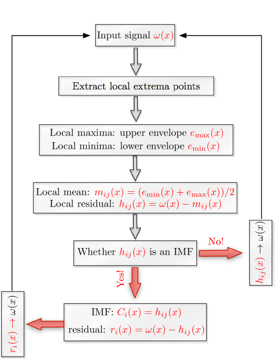
Figure 1: (Color online) A flowchart of the Empirical Mode Decomposition algorithm to show how to decompose a given vortex filed $\omega(x,y)$ at certain $y$ into a sum of Intrinsic Mode Functions $C_{i}(x)$.

II.1 Empirical Mode Decomposition

The method we used in this work is the so-called arbitrary-order Hilbert spectral analysis. Huang et al. (2008, 2011) It is an extended version of the Hilbert-Huang Transform (HHT). Huang et al. (1998); Huang, Shen, and Long (1999) The Hilbert method contains two steps. In the first step, a data-driven algorithm, namely Empirical Mode Decomposition (EMD), is designed to decompose a given signal, e.g., $\omega(x)$, into a sum of Intrinsic Mode Functions (IMFs) $C_{i}(x)$ without a priori basis. Huang et al. (1998); Flandrin and Gonçalvès (2004) The IMF is an approximation of the mono-component signal, which has to satisfy the following two conditions: (i) the difference between the number of local extrema and the number of zero-crossings must be zero or one; (ii) the running mean value of the envelope defined by the local maxima and the envelope defined by the local minima is zero. (Huang et al., 1998; Huang, Shen, and Long, 1999; Rilling, Flandrin, and Gonçalvès, 2003) The extracted IMF mode possesses a well-behave Hilbert spectrum with a physical meaningful instantaneous frequency in time domain (resp. wavenumber in space domain).Huang et al. (1998); Huang, Shen, and Long (1999) Figure 1 shows a flowchart of the EMD algorithm to demonstrate how to decompose a given vortex signal $\omega(x)$ into a sum of IMF modes, i.e.,

$$\omega(x)=\sum_{i=1}^{N}C_{i}(x)+r_{N}(x)$$ (4)

in which $r_{N}(x)$ is residual. There exist several criteria to stop the sifting process and to determine whether an IMF mode is retrieved.Huang et al. (1998); Huang, Shen, and Long (1999); Rilling, Flandrin, and Gonçalvès (2003) For example, Huang et al. (1998) has proposed a Cauchy like criteria computed from two consecutive sifting, i.e.,

$$SD=\frac{\int\left[h_{i(j-1)}(x)-h_{ij}(x)\right]^{2}\mathrm{\,d}x}{\int\left[h_{i(j-1)}(x)\right]^{2}\mathrm{\,d}x}$$ (5)

in which $h_{ij}(x)$ is the residual by removing the running mean $m_{ij}(x)$ constructed by using upper $e_{\max}(x)$ and lower envelopes $e_{min}(x)$. Here $e_{\max}(x)$ (resp. $e_{\min}(x)$) is the upper envelope constructed by using the local maxima points (resp. minima points). A typical value can be set between $0.2$ and $0.3$ to provide a physical meaningful IMF mode. Another widely used stopping criteria is proposed by Rilling, Flandrin, and Gonçalvès (2003). They introduced an amplitude function $a(x)=(e_{\max}(x)-e_{\min}(x))/2$ and an evaluation function $\sigma(x)=m_{ij}(x)/a(x)$, respectively. The sifting procedure is iterated until $\sigma(x)<\theta_{1}$ for some prescribed fraction $(1-\alpha)$ of the total data, while $\sigma(x)<\theta_{2}$ for the rest fraction. Typical values are $\alpha\simeq 0.05$, $\theta_{1}\simeq 0.05$ and $\theta_{2}\simeq 10\theta_{1}$.Rilling, Flandrin, and Gonçalvès (2003) A maximum iteration number, i.e., $100$, could also be used to stop the sifting. In our practice, any one of the above three criteria is satisfied, then one IMF mode is retrieved.

II.2 Hilbert Spectral Analysis

After retrieving the IMF modes, the Hilbert spectral analysis is applied to each mode to obtain the time-frequency information. Huang et al. (1998); Huang, Shen, and Long (1999); Huang (2009) The Hilbert transform is defined as, i.e.,

$$\overline{C}_{i}(x)=\frac{1}{\pi}P\int\frac{C_{i}(x^{\prime})}{x-x^{\prime}}\mathrm{\,d}x^{\prime}$$ (6)

in which $P$ means the Cauchy principle value.Cohen (1995); Flandrin (1998) A so-called analytical signal is then written as, i.e.,

$$C_{i}^{A}(x)=C_{i}(x)+j\overline{C}_{i}(x)$$ (7)

in which $j=\sqrt{-1}$. An instantaneous wavenumber is then defined as, i.e.,

$$k_{i}(x)={\frac{1}{2\pi}}\frac{\mathrm{\,d}}{\mathrm{\,d}x}\arctan\left(\frac{\overline{C}_{i}(x)}{C_{i}(x)}\right)$$ (8)

Note that Eq. (6) is a singularity transform. The differential operation is also used to define the instantaneous wavenumber, see Eq. (8). Therefore, the Hilbert method possesses a very local ability in the wavenumber domain. The final representation of the original data $\omega(x)$ can be written as, i.e.,

$$\omega(x)=\sum_{i=1}^{N}\mathcal{A}_{i}(x)\exp\left(\int_{-\infty}^{x}jk_{i}(x^{\prime}{})\mathrm{\,d}x^{\prime}{}\right)$$ (9)

in which $\mathcal{A}_{i}(x)=\sqrt{\overline{C}_{i}(x)^{2}+C_{i}(x)^{2}}$ is the modulus of $C_{i}^{A}(x)$. Huang et al. (1998, 2011) Comparison with the Fourier analysis, the above representation can be considered as a local Fourier expansion, in which the amplitude $\mathcal{A}$ and wavenumber $k$ can be varied with $x$, namely amplitude- and frequency-modulation.Huang et al. (1998)

II.3 Arbitrary Order Hilbert Spectral Analysis

After obtaining the IMF modes $C_{i}(x)$ and the corresponding instantaneous wavenumber $k_{i}(x)$, one can construct a set of pair $[C_{i}(x),k_{i}(x)]$. A $k$-conditional $q$th-order statistical moment is then defined as, i.e.,

$$\mathcal{L}_{q}(k)=\langle\sum_{i=1}^{N}\left[C_{i}(x)|_{k_{i}(x)=k}\right]^{q}\rangle_{x}$$ (10)

in which $\langle\cdots\rangle$ is ensemble average over all $i$ and $x$. Huang et al. (2011, 2013) $\mathcal{L}_{q}(k)$ could be defined by another equivalent way as described below. One can extract a joint probability density function (pdf) i.e., $p(C,k)$, from the IMF mode $C_{i}(x)$ and the corresponding wavenumber $k_{i}(x)$. Taking a marginal integration, Eq. (10) is then rewritten as, i.e.,

$$\mathcal{L}_{q}(k)=\frac{\int p(C,k)|C|^{q}{\color[rgb]{0,0,0}\mathrm{\,d}C}}{\int p(C,k){\color[rgb]{0,0,0}\mathrm{\,d}C}}$$ (11)

For a scaling process, one expects a power-law behavior, i.e.,

$$\mathcal{L}_{q}(k)\sim k^{-\zeta(q)}$$ (12)

in which $\zeta(q)$ is comparable with the scaling exponents provided by the classical structure function.Huang et al. (2011)

The Hilbert-based methodology has been verified by using a synthesized fractional Brownian motion data for mono-fractal process and a synthesized multifractal random walk with a lognormal statistics for multifractal process. Huang et al. (2011) It also has been applied successfully to turbulent velocity,Huang et al. (2008) passive scalar, Huang et al. (2010) Lagrangian turbulence,Huang et al. (2013) etc., to characterize the intermittent nature of those processes. Our experience is that the SF analysis works when $1<\beta<3$ without energetic structures.Huang et al. (2010) Here $\beta$ is the scaling exponent of Fourier power spectrum, i.e., $E(k)\sim k^{-\beta}$. If $\beta$ is out of this range, then the Hilbert methodology should be applied to extract scaling exponents for high-order $q$. Moreover, due to the influence of energetic structures, the SFs may fail even when $\beta=2$. This has been found to be the case of the three-dimensional Lagrangian turbulence.Huang et al. (2013) We will show below that this is also the case of 2D turbulence, see more discussion in Sec. III.2. For more detail about the methodology we refer the reader to the Refs. Huang et al., 1998, 2008; Huang, 2009; Huang et al., 2011, 2013.

III Numerical Data and scaling of high-order statistics

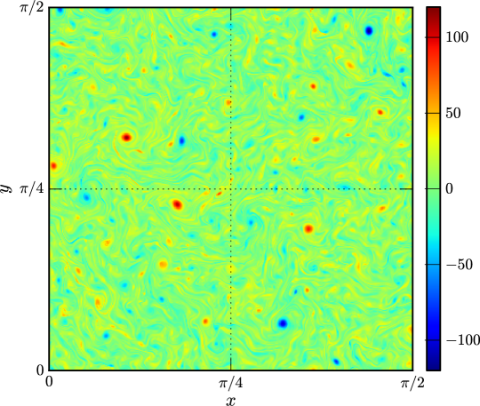
Figure 2: (Color online) A snapshot of the vorticity field $\omega(x,y)$ of the two-dimensional turbulence on the range $0\leq x,y\leq\pi/2$ from a high resolution direct numerical simulation with $8192^{2}$ grid points. High intensity vorticity events are discrete distributed in space with a typical wavenumber $k\simeq k_{f}=100$ (resp. around $80$ grid points).

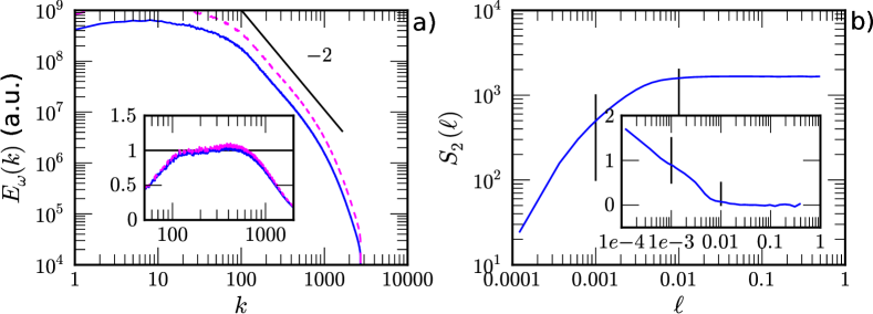
Figure 3: (Color online) a) Measured Fourier power spectrum $E_{\omega}(k)$ for vorticity field $\omega(x,y)$, in which a logarithmic correction $E_{\omega}(k)\ln(k/k_{\min})^{-1/3}$ is shown as a dashed line. For display clarity, the measured $E_{\omega}(k)\ln(k/k_{\min})^{-1/3}$ has been vertical shifted by multiplying a factor 5. A nearly one decade power-law behavior is found on the wavenumber range $100\leq k\leq 1000$, corresponding to $0.001\leq\ell\leq 0.01$ with a scaling exponent $\beta=1.96\pm 0.02$ for $E_{\omega}(k)$ and $\beta=2.02\pm 0.02$ for $E_{\omega}(k)\ln(k/k_{\min})^{-1/3}$, respectively. The inset shows the compensated spectrum with fitted scaling exponents. This scaling range corresponds to the forward enstrophy cascade. b) Measured second-order structure-function $S_{\omega}(2,\ell)$. No power-law behavior is observed as expected on the range $0.001\leq\ell\leq 0.01$. The inset shows the local slope $\zeta_{\omega}(2,\ell)=\mathrm{\,d}\log_{10}S_{\omega}(2,\ell)/\mathrm{\,d}\log_{10}\ell$ to confirming the lacking of the power-law behavior.

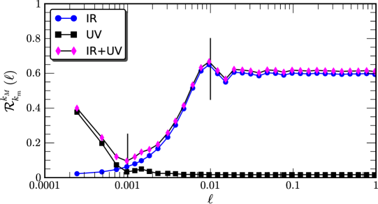
Figure 4: (Color online) Measured relative contribution function $\mathcal{R}^{k_{M}}_{k_{m}}(\ell)$ from different Fourier modes. Low wave number part (IR) $[0,100]$ ($\ocircle$), high wavenumber part (UV) $[1000,+\infty]$ ($\square$). The expected power-law range is illustrated by a vertical solid line. Note that the expected power-law behavior is strong influenced by the low wavenumber part, known as IR effect.

III.1 Direct Numerical Simulation of 2D Turbulence

The DNS data we used in this study is provided by Professor G. Boffetta. We recall briefly several key parameters of this simulation. Numerical integration of Eq. (1) is performed by a pseudo-spectral, fully dealiased on a doubly periodic square domain of size $L=2\pi$ at resolution $N^{2}=8192^{2}$ grid points. Boffetta (2007) The main parameters are respectively $\nu=2\times 10^{-6}$, $\alpha=0.025$ and $k_{f}=100$, in which the energy is inputed into the system. The velocity field $\mathbf{u}=\nabla\times\Phi$ is then obtained by solving a Poisson problem $\nabla^{2}\Phi=-\omega$, in which $\Phi$ is a stream function. Totally, we have five snapshots with $8192^{2}\times 5=3.36\times 10^{8}$ data points. In the following, the analysis is done along the $x$-direction. This provides $8192\times 5=40960$ realizations for each statistics. The ensemble average is then averaged from all these realizations. Figure 2 shows a portion of one snapshot of the vorticity field. Note that high intensity events are discrete distributed in physical space with a typical wavenumber $k\simeq k_{f}=100$ (resp. $\sim 80$ grid points). More detail of this database can be found in Ref. Boffetta, 2007.

III.2 Fourier Power Spectrum and Second-Order Structure-Function

Figure 3 a) shows the measured Fourier power spectrum $E_{\omega}(k)$ (solid line) of the vorticity field, in which the logarithmic correction $E_{\omega}(k)\ln(k/k_{\min})^{-1/3}$ is shown as a dashed line. A power-law behavior for the forward enstrophy cascade is observed on the range $100\leq k\leq 1000$, i.e., $E_{\omega}(k)\sim k^{-\beta}$, with a scaling exponent $\beta=1.96\pm 0.02$. The measured $\beta$ is consisted with the one reported by Kellay, Wu, and Goldburg (1998). The observed scaling range corresponds to a spatial scale range $0.001\leq\ell\leq 0.01$. The logarithmic correction provides a scaling exponent $\beta=2.02\pm 0.02$ on the same scaling range, showing a weak correction of the power-law behavior.Pasquero and Falkovich (2002) The inset shows the corresponding compensated curves to emphasize the observed power-law behavior. We therefore expect a power-law behavior on the range $0.001\leq\ell\leq 0.01$ for the second-order SFs, i.e.,

$$S_{\omega}(2,\ell)=\langle|\Delta_{\ell}\omega|^{2}\rangle\sim\ell^{\beta-1}$$ (13)

in which $\Delta_{\ell}\omega=\omega(x+\ell)-\omega(x)$ is vorticity increment, and $\beta$ is the scaling exponent from $E_{\omega}(k)\sim k^{-\beta}$. Figure 3 b) shows the measured second-order SF, in which the forward enstrophy cascade is illustrated by a vertical solid line. Visually, no power-law behavior is observed for the measured $S_{\omega}(2,\ell)$ for the forward enstrophy cascade. To emphasize this point, the local slope, i.e., $\zeta_{\omega}(2,\ell)=\mathrm{\,d}\log_{10}S_{\omega}(2,\ell)/\mathrm{\,d}\log_{10}\ell$, is shown in the inset. There is no plateau observed on the range of the forward enstrophy cascade, showing the failure of the SFs to capture the scale invariance of the two-dimensional vorticity field.

To understand more about the second-order SFs $S_{\omega}(2,\ell)$, one can relate it with the Fourier power spectrum by using Wiener-Khinchin theorem,Frisch (1995); Huang et al. (2010) i.e.,

$$S_{\omega}(2,\ell)=\int_{0}^{+\infty}E_{\omega}(k)(1-\cos(2\pi k\ell))\mathrm{\,d}k$$ (14)

in which $E_{\omega}(k)$ is the corresponding Fourier power spectrum. Note that an integral constant is neglected since it does not change the conclusion in this paper. The above equation implies that the SFs contains contribution from almost all Fourier modes $k$. The expected power-law behavior might be influenced by both large-scale (resp. low wavenumber, known as infrared effect, IR) and small-scale (resp. high wavenumber, known as ultraviolet effect, UV) motions. A partial cumulative function is therefore introduced to characterize a relative contribution from Fourier modes band $[k_{m},k_{M}]$, i.e.,

$$\mathcal{R}_{k_{m}}^{k_{M}}(\ell)=\frac{\int_{k_{m}}^{k_{M}}E_{\omega}(k^{\prime}{})(1-\cos(2\pi k^{\prime}{}\ell))\mathrm{\,d}k^{\prime}{}}{\int_{0}^{+\infty}E_{\omega}(k)(1-\cos(2\pi k\ell))\mathrm{\,d}k}$$ (15)

We are particular concerned by the Fourier modes below the forcing scale,i.e., $[0,100]$ (resp. IR) and by the modes above the power-law range, i.e., $[1000,+\infty]$ (resp. UV). Figure 4 shows the measured $\mathcal{R}_{m}^{M}(\ell)$ for IR ($\ocircle$) and UV ($\square$). It indicates that the SFs is strongly influenced by the large-scale motions (resp. IR) as high as up to $65\%$. The expected power-law behavior is then destroyed.Davidson and Pearson (2005); Huang et al. (2010)

We provide some comments on the above analysis here. The Wiener-Khinchin theorem is only exactly valid for the linear and stationary processes. Turbulent signals in 3D or 2D are typical nonlinear and nonstationary ones. Therefore, the above argument holds approximately here. However, this does not change the conclusion of this paper. Another comment is for the observed high intensity vorticity event, see Fig. 2. For the high-order SFs, they might be also influenced by those events since they usually manifest themselves at the pdf tail of vorticity increments. This has been observed for the Lagrangian turbulence, in which the high intensity event is known as ‘vortex trapping’ process.Toschi et al. (2005); Huang et al. (2013)

III.3 Generalization Scaling for High-Order Statistics

Assuming that we have SFs scaling for both the inverse and forward cascades. The corresponding SFs and their scaling exponents without intermittent corrections are

$$S_{u}(q,\ell)\sim\left\{\begin{array}[]{lll}&\ell^{q/3},&\textrm{{\color[rgb]{0,0,0}for inverse energy cascade}}\\ &\ell^{q},&\textrm{for forward enstrophy cascade}\end{array}\right.$$ (16a)

for the velocity field,Falkovich and Lebedev (1994) and

$$S_{\omega}(q,\ell)\sim\ell^{-q}S_{u}(q,\ell)\sim\left\{\begin{array}[]{lll}&\ell^{-2q/3},&\textrm{{\color[rgb]{0,0,0}for inverse energy cascade}}\\ &\ell^{0},&\textrm{for forward enstrophy cascade}\end{array}\right.$$ (16b)

for the vorticity field. It implies that the forward enstrophy cascade represented by the vorticity field is independent on the separation scale $$\ell$$. In the frame of Hilbert, we expect the following scaling behavior for the vorticity field, i.e.,

$$\mathcal{L}_{\omega}(q,k)\sim\left\{\begin{array}[]{lll}&k^{2q/3},&\textrm{{\color[rgb]{0,0,0} for inverse energy cascade}}\\ &k^{0},&\textrm{ for forward enstrophy cascade}\end{array}\right.$$ (16c)

We will then test above relation by using the Hilbert method as we described above.

IV Hilbert Results and Discussion

IV.1 Hilbert Statistics

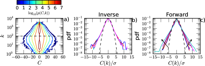
Figure 5: (Color online) a) Contour plot of measured conditional histogram $p(C,k)$ (resp. joint probability density function (pdf)), in which the force scale is illustrated by a dashed line. b) Measured pdf $p(C)$ on the range $3<k<20$ (resp. $k=4,6,16$ and $20$) for the inverse energy cascade . c) Measured pdf $p(C)$ on the range $200<k<2000$ (resp. $k=250,400,800,1000$ and $1600$) for the forward enstrophy cascade. For comparison, the normal distribution is illustrated by a dashed line.

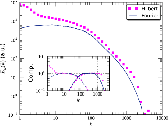
Figure 6: (Color online) Comparison of the measured Hilbert energy spectrum $\mathcal{L}_{2}(k)/k$ ($\square$) and the Fourier energy spectrum $E_{\omega}(k)$ (solid line). For display clarity, the curves have been vertical shifted. Inset shows the corresponding compensated spectra for both inverse energy cascade and forward enstrophy cascade by using fitting scaling exponents respectively on the range $3<k<20$ and $100<k<1000$.

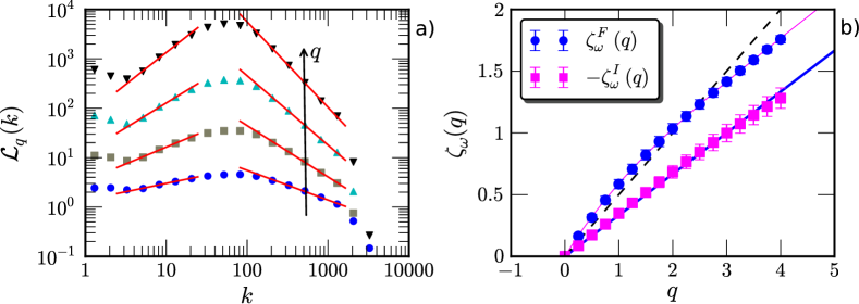
Figure 7: (Color online) a) Measured $q$th-order Hilbert spectra $\mathcal{L}_{q}(k)$ for $q=1,2,3,4$. power-law behavior is observed on the range $200\leq k\leq 2000$ for the forward enstrophy cascade and on the range $3\leq k\leq 20$ for the inverse energy cascade, respectively. The scaling exponents $\zeta_{\omega}(q)$ are then estimated on this dual power-law ranges. b) Measured scaling exponents $\zeta_{\omega}^{F}(q)$ ($\ocircle$) and $-\zeta_{\omega}^{I}(q)$ ($\square$). For comparison, the dashed line is $q/3$ and the solid line is for a log-Poisson fitting $\zeta_{\omega}^{F}(q)=q/3+0.45(1-0.43^{q})$. The errorbar indicates $95\%$ fitting confidence.

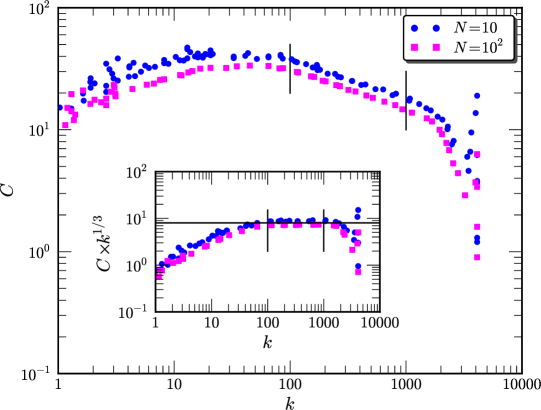
Figure 8: (Color online) Experimental contour line for $N=10$ ($\ocircle$) and $N=100$ ($\square$). power-law behavior is observed on the range $100\leq k\leq 1000$ with a scaling exponent $\simeq 1/3$. The inset shows the compensated curve by multiplying $k^{1/3}$. The observed power-law indicates an asymptotic scaling exponent $\lim_{q\rightarrow+\infty}\zeta_{\omega}^{F}(q)=q/3$.

The Hilbert method is applied to the vorticity field $\omega(x,y)$ along $x$-direction. The conditioned/joint histogram $p(C,k)$ (resp. probability density function if it is renormalized properly) is extracted from all five snapshots. Figure 5 a) shows the contour plot of the measured $p(C,k)$, in which the forcing scale $k_{f}=100$ is illustrated by a horizontal dashed line. For display clarity, we take the logarithm of the measured $p(C,k)$. It is interesting to note that the joint pdf is roughly separated by the forcing wavenumber $k_{f}=100$ into two regimes. The first regime is on the range $2\leq k\leq 20$, corresponding to the inverse energy cascade. The another one is on the range $200\leq k\leq 2000$, corresponding to the forward enstrophy cascade. Figure 5 b) shows the pdf $p(C|k)$ on the inverse energy cascade (resp. $k=4,6,16$ and $20$ ). For comparison, the normal distribution is demonstrated by a solid line. All the measured pdf has an exponential tail. We note that the pdf in the inverse energy cascade does collapse with each other, indicating a nonintermittent cascade. For the pdf in the forward enstrophy cascade, they also possess an exponential tail. However, they can not collapse with each other due to different shape of the core part $-5<C(k)/\sigma<5$. The exponential tail of the vorticity field consists with very recently theoretical prediction by Falkovich and Lebedev (2011).

Figure 6 shows the comparison of the measured Hilbert energy spectrum $\mathcal{L}_{2}(k)/k$ ($\square$) and the Fourier power spectrum $E_{\omega}(k)$ (solid line). For display clarity, the curve has been vertical shifted. Note that both methods provide the nearly same forward enstrophy cascade on the range $100<k<1000$ with a scaling exponent close to $\simeq 2$. This scaling exponent agrees very well with the experimental observation by Kellay, Wu, and Goldburg (1998). We show in the inset the compensated curve by using the fitted exponent for the forward cascade (closed square for the Hilbert and solid line for Fourier). The observed plateau confirms the power-law behavior as expected. Furthermore, we have an additional power-law behavior on the range $3<k<20$ for the inverse energy cascade. The compensated spectra are also shown in the inset (open square for the Hilbert and dashed line for Fourier) to emphasize the observed inverse energy cascade. Both Hilbert and Fourier methodologies identify almost the same dual power-law behavior.

We now turn to the high-order Hilbert statistics. The convergence of the statistical moment $\mathcal{L}_{q}(k)$ has been verified by checking the integral kernel $p(C,k)|C|^{q}$ at given scales. A quite good convergence has been found for all wavenumber $k$ up to $q=4$ (not shown here). Figure 7 a) shows the measured $\mathcal{L}_{q}(k)$ for $q=1,2,3$ and $4$ (from bottom to top). A dual power-law behavior is observed as expected respectively on the range $3\leq k\leq 20$ for the inverse energy cascade and $200\leq k\leq 2000$ for the forward enstrophy cascade. The scaling exponent $\zeta_{\omega}(q)$ is then estimated respectively on these two ranges by using a least square fitting algorithm. Figure 7 b) shows the corresponding measured scaling exponent $\zeta_{\omega}(q)$, in which the errorbar is 95% fitting confidence. For the inverse energy cascade, the measured $\zeta_{\omega}^{I}(q)$ ($\square$) is linear with $q$, i.e., $\zeta_{\omega}^{I}(q)=-q/3$, confirming that there is no intermittent effect in this inverse cascade process.Boffetta and Ecke (2012) However, the observed $-q/3$ scaling does not consist with the prediction of Eq. (16c). This implies that for the vorticity field some important mechanisms are ignored in the previously dimensional arguments of the inverse energy cascade. For example, if one takes the enstrophy dissipation $\eta_{\alpha}$ into account and assumes it as important as the Ekman energy dissipation $\epsilon_{\alpha}$, one then has the right scaling behavior, i.e., $\mathcal{L}_{q}(k)\sim\left(\epsilon_{\alpha}\eta_{\alpha}\right)^{q/6}k^{q/3}$. This corresponds to a scaling exponent $\zeta_{\omega}^{I}(q)=-q/3$ for the inverse energy cascade. However, this naive dimensional argument should be justified for physical evidence and for more database.

The measured scaling exponent $\zeta_{\omega}^{F}(q)$ ($\ocircle$) is also shown in Fig. 7 b). We note that when $q\leq 2$ the measured $\zeta_{\omega}^{F}(q)$ is nonlinear dependent with $q$, indicating an intermittent effect of the vorticity field. While when $q\geq 2$, it seems to be linear with $q$ with a slope $\simeq 1/3$. We propose here a log-Poisson-like model for the observed scaling exponent, i.e.,

$$\zeta_{\omega}^{F}(q)=\gamma q+\mathcal{B}\left(1-\varphi^{q}\right)$$ (17)

in which the parameter $\gamma=1/3$, $\mathcal{B}=0.45$ and $\varphi=0.43$ are determined as following. For large value of $q$ (if the corresponding statistics exists), the $q$th-order Hilbert moments $\mathcal{L}_{q}(k)$ is thus dominated by the tail of the pdf $p(C,k)$. Therefore, if the scaling behavior holds, the measured joint pdf $p(C,k)$ should also show a scaling behavior for the contour line. We extract the measured contour line for $p(C,k)$ (in points) with two values $N=10$ ($\ocircle$) and $100$ ($\square$), see Fig. 8. Power-law behavior is indeed observed as expected on the range $100\leq k\leq 2000$. The scaling exponent is found to be $\simeq 1/3$. To emphasize the observed $1/3$ scaling, the compensated curves $C(k)k^{1/3}$ are shown as inset of Fig. 8. A clear plateau is observed on the expected range $100\leq k\leq 2000$. This yields $\gamma=1/3$. The rest of the parameters $\mathcal{B}$ and $\varphi$ are then obtained by using a least square fitting algorithm.

IV.2 Extended Self-Similarity of Structure-Functions

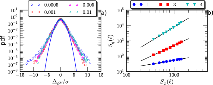
Figure 9: (Color online) a) Measured pdf for vorticity increments with several separation scales $\ell$ in the range of the forward enstrophy cascade. The Gaussian distribution is illustrated by a solid line. Note that except for the first scale ($\ell=0.0005$), they all have an exponential tails and do collapse with each other. b) Extended Self-Similarity plots of the SFs on the range $0.0005<\ell<0.005$, corresponding to a wavenumber range $200<k<2000$. The solid line is a power-law fitting on this range by using a least square algorithm. For display clarity, these curves have been vertical shifted.

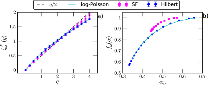
Figure 10: (Color online) a) Comparison of the measured relative scaling exponents $\zeta_{\omega}^{E}(q)$ for the SFs ($\square$), the scaling exponent $\zeta_{\omega}^{F}(q)$ provided by the Hilbert method ($\ocircle$) and the log-Poisson fitting (solid line). b) The corresponding singularity spectrum $f_{\omega}(\alpha)$.

As we shown above that due to the large-scale structure influence the second-order SF fails to identify the power-law behavior of the forward enstrophy cascade, see Fig. 3 b). Here we apply the Extended Self-Similarity (ESS) technique to extract the relative scaling exponents.Benzi et al. (1993) Note that for the forward enstrophy cascade, the second-order Hilbert moments provides a scaling exponent $\zeta^{F}_{\omega}(2)\simeq 1$ and the Fourier power spectrum provides $\beta\simeq 2$. Therefore, we define the ESS of the SFs by using the second-order SFs, i.e.,

$$S_{q}(\ell)\sim\left(S_{q}(\ell)\right)^{\zeta^{E}_{\omega}(q)}$$ (18)

in which $S_{q}(\ell)=\langle|\Delta_{\ell}\omega|^{q}\rangle$, and $\zeta^{E}_{\omega}(q)$ is the ESS scaling exponent. Figure 9 a) shows the measured pdf of the vorticity increment for different separation scales in the forward enstrophy cascade. Except for $\ell=0.005$, all the pdfs have an exponential tail and almost collapse with each other. Figure 9 b) shows the ESS plots on the range $0.0005<\ell<0.005$, corresponding to a wavenumber range $200<k<2000$, which is the scaling range of the forward enstrophy cascade predicted by the Hilbert method. Power-law behavior is observed for all $q$ we considered here. The ESS scaling is estimated on this range by using a least square fitting algorithm. Figure 10 a) shows the measured ESS scaling exponent $\zeta_{\omega}^{E}(q)$ ($\square$), in which the errorbar indicates the 95% fitting confidence. For comparison, the scaling exponent provided by the Hilbert method ($\ocircle$) is also shown. Graphically, the measured $\zeta^{E}_{\omega}(q)$ indicates a less intermittent vorticity field. To emphasize this point, the singularity spectrum $f_{\omega}(\alpha)$ is then calculated, i.e.,

$$\alpha_{\omega}=\zeta_{\omega}(q)^{\prime}{},\,\quad f_{\omega}(\alpha)=\min\left\{\alpha_{\omega}q-\zeta_{\omega}(q)+1\right\}$$ (19)

in which the scaling exponents $\zeta_{\omega}(q)$ could be either scaling exponent from Hilbert method or one from the SFs. Figure 10 b) shows the measured $f_{\omega}(\alpha)$ for the forward enstrophy cascade, in which the log-Poisson fitting is illustrated by a solid line. It confirms again that the SFs predicts a less intermittent vorticity field.

IV.3 Discussion

Several works have been reported for the forward enstrophy cascade that the Fourier power spectrum of vorticity field possesses a ‘$-2$’ power-law behavior rather than ‘$-1$’ one required by Kraichnan’s theory, see Eq. (3). However, there is no theory explanation for this contradiction. Specifically for the Hilbert method, we note that the second-order statistics $\mathcal{L}_{2}(k)$ provides $\zeta_{\omega}^{F}(2)\simeq 1.0$ (resp. ‘$-2.0$’ for the Hilbert energy spectrum) rather than $0$ required by the dimensional argument. The high-order scaling exponents $\zeta_{\omega}(q)$ provided by the Hilbert method for both the inverse energy cascade and forward enstrophy cascade disagree with the Kraichnan’s theory prediction, see Eq. (16).Kraichnan (1967); Falkovich and Lebedev (1994) Furthermore, they do not agree with the logarithmic correction theory either.Falkovich and Lebedev (1994) It suggests that a new theory is required in future to interpret the vorticity field of 2D turbulence to take into account not only this inconsistence but also the intermittent effect.

We emphasize here that the scaling property of the forward enstrophy cascade might depend on the Ekman friction, the parameter $\alpha$. Boffetta et al. (2002); Biferale et al. (2003); Boffetta (2007) Therefore, more data sets should be certainly investigated in future to see whether the scaling behavior reported in this work is universal for different $\alpha$.

V Conclusion

In summary, we have applied the Hilbert methodology to the vorticity field obtained from a high resolution DNS of 2D turbulence. A dual-cascade with almost one decade scales for the inverse energy cascade and forward enstrophy cascade is identified. The scaling exponents $\zeta_{\omega}(q)$ are extracted. In the inverse energy cascade, the pdf $p(C,k)$ is collapsed with each other with an exponential tail. This indicates a nonintermittent cascade process, which is confirmed by the measured scaling exponent $\zeta_{\omega}^{I}(q)=-q/3$. In the forward enstrophy cascade, the measured pdf $p(C,k)$ also have an exponential tail. However, due to the different shape of the core part, they can not collapse with each other, indicating an intermittent forward enstrophy cascade. The measured scaling exponent $\zeta_{\omega}^{F}(q)$ is nonlinear with $q$ when $q\leq 2$, showing intermittency. A log-Poisson fitting, i.e., $\zeta_{\omega}^{F}(q)=q/3+0.45(1-0.43^{q})$, is thus proposed to characterize the measured $\zeta_{\omega}^{F}(q)$.