Time dependent intrinsic correlation analysis of temperature and dissolved oxygen time series using empirical mode decomposition

Abstract

In the marine environment, many fields have fluctuations over a large range of different spatial and temporal scales. These quantities can be nonlinear and non-stationary, and often interact with each other. A good method to study the multiple scale dynamics of such time series, and their correlations, is needed. In this paper an application of an empirical mode decomposition based time dependent intrinsic correlation, of two coastal oceanic time series, temperature and dissolved oxygen (saturation percentage) is presented. The two time series are recorded every 20 minutes for 7 years, from 2004 to 2011. The application of the Empirical Mode Decomposition on such time series is illustrated, and the power spectra of the time series are estimated using the Hilbert transform (Hilbert spectral analysis). Power-law regimes are found with slopes of 1.33 for dissolved oxygen and 1.68 for temperature at high frequencies (between 1.2 and 12 hours) with both close to 1.9 for lower frequencies (time scales from 2 to 100 days). Moreover, the time evolution and scale dependence of cross correlations between both series are considered. The trends are perfectly anti-correlated. The modes of mean year 3 and 1 year have also negative correlation, whereas higher frequency modes have a much smaller correlation. The estimation of time-dependent intrinsic correlations helps to show patterns of correlations at different scales, for different modes.

1 Introduction

Generally in geosciences, but especially in the marine environment, many fields have fluctuations over a large range of spatial and temporal scales. To study their dynamics and estimate their variations at all scales, high frequency measurements are needed (Dickey, 1991; Chavez, 1997; Chang and Dickey, 2001). Here a time series obtained from automatic measurements in a moored buoy station in coastal waters of Boulogne-sur-mer (eastern English Channel, France) is considered, recorded every 20 minutes from 2004 to 2011 (Zongo and Schmitt, 2011; Zongo et al., 2011). This fixed buoy station can record various biogeochemical parameters simultaneously. Here, mainly to illustrate the application of a new method for multi-scale data analysis there is a focus on two parameters: temperature, due to its obvious importance, influenced by the dynamics, by meteorology, and as a link with ecosystem forcing, and dissolved oxygen time series, due to its important role in biological processes, and also for the probable growing importance of this parameter to assess the quality of coastal waters, in the framework of European directives (Best et al., 2007).

These physical and biogeochemical time series are nonlinear, and non-stationary, and may possess interactions at different scales. In order to consider their multi-scale dynamic properties and explore their correlations at different scales, the Empirical Mode Decomposition (EMD) framework is applied here (Huang et al., 1998).

EMD and the associated Hilbert spectral analysis (resp. Hilbert-Huang Transform, HHT) have already been applied in marine sciences, (Hwang et al., 2003; Dätig and Schlurmann, 2004; Veltcheva and Soares, 2004; Schmitt et al., 2009). For example, Hwang et al. (2003) applied the HHT method to ocean wave data. They found that the HHT method detects more energy in lower frequencies, leading to a lower average frequency in HHT spectra than using the Fourier framework. Dätig and Schlurmann (2004) showed that the HHT method can used to study nonlinear waves using instantaneous frequencies. Schmitt et al. (2009) applied the HHT method to characterize the scale invariance of velocity fluctuations in the surf zone. They observed that the scale invariance holds for almost two decades of time scales.

In the following, the methodology is presented and then its application is illustrated on the chosen time series. Section 2 presents the Hilbert-Huang Transform method and the fairly recent time dependent intrinsic correlation; section 3 presents the data base; section 4 presents the analysis of the intrinsic correlation and section 5 draws the main conclusion of this paper.

2 Hilbert-Huang Transform and Time Dependent Intrinsic Correlation

In this section, the Hilbert-Huang Transform and the empirical mode decomposition based time dependent intrinsic correlation are presented. These time series analysis techniques have been applied, since their introduction in 1998 (Huang et al., 1998), in several thousand different studies in natural and applied sciences. Here the main idea is recalled but the method is not presented in too much detail.

The HHT consists of two steps. The first step is the so-called ‘empirical mode decomposition’, which separates a multi-scale time series into a sum of intrinsic mode functions without a priori basis assumption (Huang et al., 1998; Flandrin and Gonçalvès, 2004). In the second step, the Hilbert spectral analysis is applied to each mode function to extract the time-frequency information. The so-called Hilbert spectrum and the corresponding Hilbert marginal spectrum are then introduced to characterize the time-frequency distribution of a given time series (Huang et al., 1998; Huang, 2009; Huang et al., 2008; Chen et al., 2010).

2.1 Empirical Mode Decomposition

Empirical Mode Decomposition is a fully adaptive technique to study the nonlinear and non-stationary properties of time series (Huang et al., 1998, 1999; Flandrin and Gonçalvès, 2004; Huang et al., 2011). The main idea of EMD is to locally separate a given multi-scale signal into a sum of a local trend and a local detail, respectively, for a low frequency part and a high frequency part (Rilling et al., 2003). The latter is called the Intrinsic Mode Function (IMF), and the former is called the residual. The procedure is repeated to the residual, considered as a new times series, extracting a new IMF using a spline function, and obtaining a new residual until no more IMF can be extracted (Huang et al., 1998, 1999; Rilling et al., 2003; Flandrin et al., 2004). The EMD method then expresses a multi-scale time series as the sum of a finite number of IMFs and a final residual (Huang et al., 1998; Flandrin et al., 2004).

To be an IMF, an approximation to the so-called mono-component signal, it must satisfy the following two conditions: (i) the difference between the number of local extrema and the number of zero-crossings must be zero or one; (ii) the running mean value of the envelope defined by the local maxima and the envelope defined by the local minima is zero (Huang et al., 1998, 1999; Rilling et al., 2003). The so-called Empirical Mode Decomposition algorithm is then proposed to decompose a signal into IMFs (Huang et al., 1998, 1999; Rilling et al., 2003):

• identify the local extrema of the signal $x(t)$;

• construct upper envelope $e_{\max}(t)$ by using the local maxima through a cubic spline interpolation (other interpolations are also possible). Construct a lower envelope $e_{\min}(t)$ by using the local minima;

• define the mean value $m_{1}(t)=(e_{\max}(t)+e_{\min}(t))/2$;

• remove the mean value from the signal, providing the local detail $h_{1}(t)=x(t)-m_{1}(t)$;

• check if the component $h_{1}(t)$ satisfies the above conditions to be an IMF. If yes, take it as the first IMF $C_{1}(t)=h_{1}(t)$. This IMF mode is then removed from the original signal and the first residual, $r_{1}(t)=x(t)-C_{1}(t)$ is taken as the new series in step 1. If $h_{1}(t)$ is not an IMF, a procedure called the “sifting process” is applied as many times as necessary to obtain an IMF (not detailed here).

By construction, the number of extrema decreases when going from one residual to the next; the above algorithm ends when the residual has only one extrema, or is constant, and in this case no more IMF can be extracted; the complete decomposition is then achieved in a finite number of steps. The analyzed signal $x(t)$ is finally written as the sum of mode time series $C_{i}(t)$ and the residual $r_{n}(t)$:

$$x(t)=\sum_{i=1}^{N}{C_{i}(t)}+r_{n}(t)$$ (1)

Based on a dyadic filter bank property of the EMD algorithm, the number of IMF modes is estimated as

$$N\leq\log_{2}(L)$$ (2)

where $L$ is the length of the data in points (Flandrin et al., 2004; Wu and Huang, 2004; Huang et al., 2008). Unlike Fourier based methodologies, e.g., Fourier analysis, wavelet transform, etc., this method does not define the basis a priori (Huang et al., 1998, 1999; Flandrin and Gonçalvès, 2004). It thus possesses full adaptability and is very suitable for non-stationary and nonlinear time series analysis (Huang et al., 1998, 1999).

2.2 Hilbert Spectral Analysis

To characterize the time-frequency distribution of the IMF mode, a complementary analysis technique namely Hilbert spectral analysis (HSA) is then applied to each IMF mode to extract the local frequency information (Long et al., 1995; Huang et al., 1998, 1999; Huang, 2009; Huang et al., 2011). In this complementary step, the Hilbert transform is used to construct the analytical signal, i.e.,

$$\tilde{C}(t)=C(t)+j\frac{1}{\pi}P\int_{-\infty}^{+\infty}\frac{C(t^{\prime}{})}{t-t^{\prime}{}}dt^{\prime}{}$$ (3)

in which $P$ is the Cauchy principle value (Cohen, 1995; Long et al., 1995; Huang et al., 1998; Flandrin, 1998). The above equation can be rewritten as

$$\tilde{C}(t)=\mathcal{A}(t)\exp(j\theta(t))$$ (4)

in which $\mathcal{A}(t)=|\tilde{C}(t)|$ is the modulus and $\theta(t)=\arctan(\mathrm{IM}(\tilde{C}(t))/\mathrm{RE}(\tilde{C}(t)))$ is the instantaneous phase function (Cohen, 1995; Long et al., 1995; Huang et al., 1998; Flandrin, 1998; Huang, 2009; Huang et al., 2011). The instantaneous frequency is then defined as

$$\omega(t)=\frac{1}{2\pi}\frac{d\theta(t)}{dt}$$ (5)

Note that the instantaneous frequency $\omega$ is very local since the Hilbert transform is a singularity transform and the differential operator is used to define the frequency $\omega$ (Huang et al., 1998, 1999; Huang, 2009). It was found experimentally that the Hilbert-based methodology is free with the Heisenberg-Gabor uncertainty and can be used to describe nonlinear distortions by using an intrawave-frequency-modulation mechanism, in which the frequency can be varied with time in one period (Huang et al., 1998; Huang, 2005; Huang et al., 2011). Therefore, the method is free with high-order harmonic components, which are required in Fourier-based methods to capture the non-stationary and nonlinear characteristics of the data (Huang et al., 1998, 1999; Huang, 2005; Huang et al., 2011).

Note that several methods exist, that could be applied to estimate the instantaneous frequency, e.g., direct quadrature, teager energy operator, etc.; see more detail in Huang et al. (2009a). In practice, the Hilbert method already provides a good estimation of $\omega$ in a statistical sense (Huang et al., 2010, 2011).

A Hilbert spectrum $H(\omega,t)=\mathcal{A}^{2}(\omega,t)$ can be designed to represent the energy of the original signal as a function of frequency $\omega$ and time. It can be taken as the best local fit to $x(t)$ using an amplitude and phase varying trigonometric function (Huang, 2005). This corresponds to a high resolution fit both in physical space and frequency space (Long et al., 1995; Huang et al., 1998). Then, the Hilbert marginal $h(\omega)$ can be defined as

$$h(\omega)=\frac{1}{T}\int_{T}H(\omega,t)\,dt$$ (6)

in which $T$ is the time period to calculate the spectrum. This is comparable to the power spectrum in Fourier analysis, but it has a quite different definition and the resulting curve would be expected to be different from the Fourier $E(f)$ curve if the times series is nonlinear and non-stationary (Huang et al., 1998). In fact, here the definition of instantaneous frequency is different from the one in the Fourier frame and the interpretation and detailed physical meaning of $h(\omega)$ is still to be fully characterized.

Another way to estimate $h(\omega)$ is based on the joint probability density function (pdf) $p(\mathcal{A},\omega)$ of amplitude $\mathcal{A}$ and the instantaneous frequency $\omega$ from all IMF modes (Huang et al., 2008; Huang, 2009; Huang et al., 2010, 2011). It is written as

$$h(\omega)=\int_{-\infty}^{+\infty}p(\mathcal{A},\omega)\mathcal{A}^{2}d\mathcal{A}$$ (7)

The combination of the EMD and HSA is then called Hilbert-Huang Transform (Huang, 2005). It has been applied successfully in various research fields to characterize the energy-time-frequency in different topics (Zhu et al., 1997; Echeverria et al., 2001; Coughlin and Tung, 2004; Loutridis, 2004; Jánosi and Müller, 2005; Molla et al., 2006a, b; Huang et al., 2008, 2009b; Schmitt et al., 2009; Chen et al., 2010), to cite a few.

2.3 Time Dependent Intrinsic Correlation

The classical global expression for the correlation, applied to non-stationary time series, may distort the true cross correlation information between time series and provide unphysical interpretation (Hoover, 2003; Rodo and Rodriguez-Arias, 2006; Chen et al., 2010). An alternative way, consistent with the possible non-stationarity of the time series, is to estimate the cross correlation coefficient by using a sliding window or a scale dependent correlation technique (Papadimitriou et al., 2006; Rodo and Rodriguez-Arias, 2006). But the main problem of these techniques is to determine how large the window should be (Chen et al., 2010). Time series from natural sciences possess fluctuations in a whole range of scales, and the data characterization must take into account this scale question (Cohen, 1995; Huang et al., 1998; Flandrin, 1998). The estimation of the cross correlation between time series, in a multi-scale framework, may use a window based on the local characteristic scale given by the data itself.

Recently, Chen et al. (2010) proposed to use the EMD to estimate an adaptive window in order to calculate a so-called time-dependent intrinsic correlation (TDIC). The TDIC of each pair of IMFs is defined as follows:

$$R_{ij}(t_{k}^{n}|t_{w}^{n})=\mathrm{Corr}\left(C_{1,i}(t^{n}_{w})C_{2,j}(t^{n}_{w})\right)\textrm{ at any }t_{k}$$ (8)

where Corr is the cross correlation coefficient of two time series and $t^{n}_{w}=[t_{k}-nt_{d}/2:t_{k}+nt_{d}/2]$ is the sliding window. The minimum sliding window size for the local correlation estimation is chosen as $t_{d}=\max(T_{1i}(t_{k}),T_{2j}(t_{k}))$, where $T_{1i}$ and $T_{2j}$ are the instantaneous periods $T=\omega^{-1}$, and $n$ is any positive real number (Chen et al., 2010). The efficiency of this approach to characterize the relation between two time series for several problems has been shown in Chen et al. (2010). Here we use this new method (with $n\geq 1$) to estimate cross correlations between coastal marine time series, where the latter can be considered as typical nonlinear and non-stationary data.

3 Presentation of the experimental database

The time series analyzed here belong to the MAREL network (Automatic monitoring network for littoral environment, Ifremer, France). Such a system is based on the deployment of moored buoys equipped with physico-chemical measuring devices, working in continuous and autonomous conditions (Woerther, 1998; Blain et al., 2004). These stations use automatic systems for seawater analysis and real time data transmission. They record several parameters, such as temperature, salinity, dissolved oxygen, pH, and turbidity, with a fixed time resolution. The measuring station used here, the MAREL Carnot station, is situated in the eastern English Channel in the coastal waters of Boulogne-sur-mer (France) at position 50.7404 N, 1.5676 W (Figure 1) and records data with a 20 minutes resolution (Zongo et al., 2011). Water depth at this position varies between 5 and 11 m; the measurements are done using a floating system inserted in a tube, 1.5m below the surface. Statistical and scaling properties of MAREL automatic measurements in the English Channel have been studied previously, considering temperature time series (Dur et al., 2007) and turbidity, oxygen and pH (Schmitt et al., 2008) in the Seine estuary, and pH fluctuations in both the Seine estuary and Boulogne-sur-mer waters (Zongo and Schmitt, 2011).

Among other parameters, the measuring buoy provides temperature, salinity and dissolved oxygen (DO) concentration data, as well as percentage of DO relative to the dissolved oxygen at equilibrium ($SaO_{2}$) for the same temperature and salinity. The DO time series is directly linked to temperature due to the solubility equation given below, whereas $SaO_{2}$ is free from such direct influence. In the following, the latter dissolved oxygen series is considered. The oxygen saturation percentage equation is given by Garcia and Gordon, as a nonlinear function of the form (Garcia and Gordon, 1992):

$$SaO_{2}=\frac{100DO}{\exp\left(P_{1}(T)+SP_{2}(T)+C_{0}S^{2}\right)}$$ (9)

where the denominator is the nonlinear fit expressing the oxygen solubility, $S$ and $T$ are salinity and temperature and $P_{1}$ and $P_{2}$ two polynomial developments ($P_{1}$ of degree five, and $P_{2}$ of degree three). Their coefficients are given in Garcia and Gordon (1992). $SaO_{2}$ data have thus no dimension and values exceeding $100\,\%$ correspond to supersaturation while values below $100\,\%$ correspond to undersaturation associated to oxygen depletion; values lower than $50\,\%$ are found for anoxic waters which can be dangerous for many species.

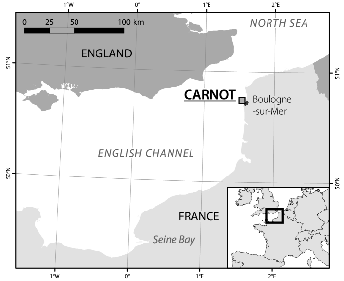
Figure 1: A map showing the measurement location Boulogne-sur-mer (France) at position 50.7404 N, 1.5676 W, in the eastern English Channel.

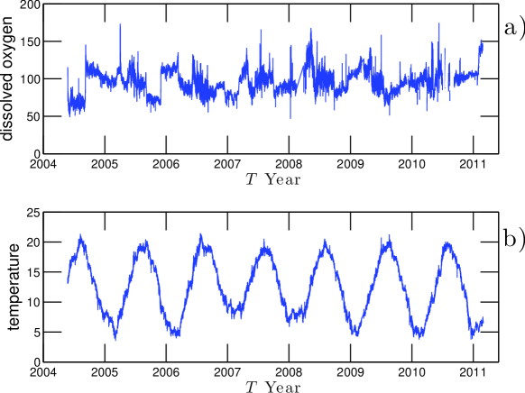
Figure 2: The observed dissolved oxygen a) and the temperature b) on the time period 25th May 2004 to 1st March 2011. Note that the sampling interval is not always 20 minutes, due to missing data. The mean period is 24 minutes for both data sets. A moderate warming winter is observed in 2007 and 2008. The observed temperature during the winter is $2\,^{\circ}\mathrm{C}$ higher than usual. Note that a strong riding-wave phenomenon is observed from January to April 2008. The observed riding-wave will cause the mode mixing problem in the EMD decomposition.

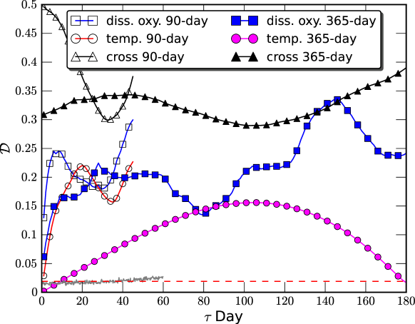
Figure 3: Statistical test of the degree of stationary $\mathcal{D}$ for the autocorrelation and cross-correlation of two data sets with a sliding window $t_{w}=90$ days and $t_{w}=365$ days. The test for white noise is illustrated as a horizontal dashed line, showing the validation of the definition of the degree of stationary. Note that the measured $\mathcal{D}$ is strongly dependent on the windows size $t_{w}$. The curves indicate that none of the series are stationary but that the temperate data set is more stationary than the dissolved oxygen one.

Due to occasional failures in the measuring system, and to regular maintenance, the time series sampling frequency is not always 20 minutes; there are frequently missing data and the mean sampling period is 24 minutes for both data sets. A total of 145,587 data points for dissolved oxygen collected from 25th May 2004 to 1st March 2011 and 155,825 data points for sea temperature collected from 24th March 2004 to 1st March 2011 have been analyzed. Figure 2 shows the two data sets. The temperature data displays a strong annual cycle. These two data sets have been analyzed on the same time period 25th May 2004 to 1st March 2011. There is a warm winter in 2007 and 2008, showing also a weak oscillation of the temperature of the sea water.

The degree of stationary which was introduced by Chen et al. (2010) is first calculated, i.e.,

$$\mathcal{D}(\tau)=\mathrm{std}\left(R(t^{n}_{k},\tau)\right)$$ (10)

in which $R(t^{n}_{k},\tau)$ is an autocorrelation function with a sliding window $t^{n}_{k}$ and time delay $\tau$. The value of $\mathcal{D}$ depends on the window size and the time delay $\tau$. It varies from $0$ to $1$ and characterizes the deviation from a stationary process (Chen et al., 2010): 0 for exactly stationary processes and the larger the value, the more it is non-stationary. Figure 3 shows the measured degree of stationary $\mathcal{D}$ for the autocorrelation and cross-correlation with a sliding window size of $t_{w}=90$ days and $t_{w}=365$ days. To show the validation of Eq. (10), a test for white noise is performed, which is illustrated by a dashed line. As expected a small value of $\mathcal{D}$ is found for white noise. These results applied on two experimental time series indicate that both are non-stationary and that the temperature is more stationary than the dissolved oxygen.

4 Analysis Results

4.1 Empirical Mode Decomposition Result

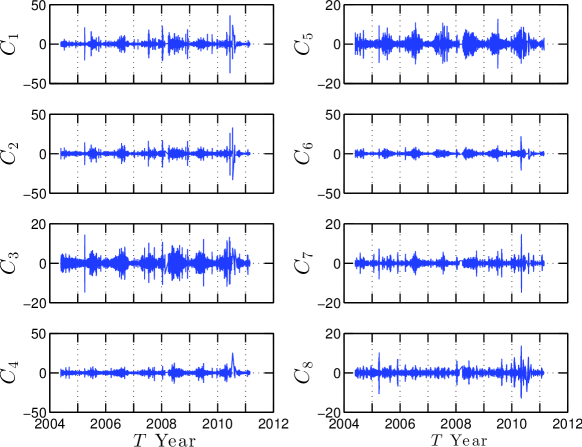
Figure 4: The first-eighth IMF modes for dissolved oxygen. The time scale is increasing with the mode index $n$.

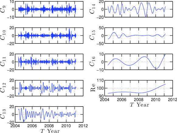
Figure 5: The last-eighth IMF modes for dissolved oxygen. The time scale is increasing with the mode index $n$.

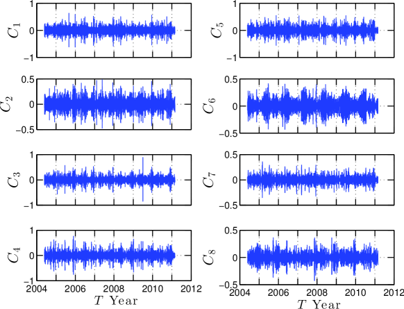
Figure 6: The first-eighth IMF modes for temperature. The time scale is increasing with the mode index $n$.

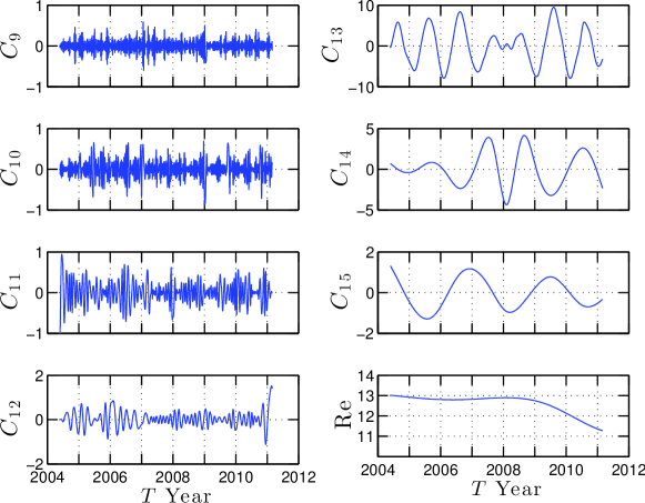
Figure 7: The last-seventh IMF modes together with the trend term for temperature. The time scale is increasing with the mode index $n$. Note that there is a serious mode mixing problem for the $13$th IMF mode around $2008$. The mean period of this mode is around 1 year. The mode mixing is caused by a riding-wave phenomenon from January 2008 to April with a typical time scale of 3 months, see Fig. 2 b.

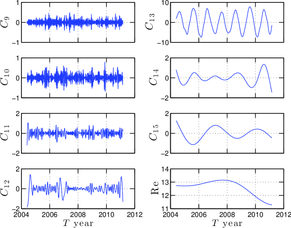
Figure 8: The last-seventh IMF modes together with the trend term for temperature by removing the riding-wave. A better annual cycle, i.e., $C_{13}$, is obtained. Note that the trend is not influenced by removing the riding-wave.

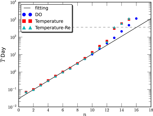
Figure 9: Mean period of IMF modes obtained for dissolved oxygen ($\ocircle$), temperature with ($\square$) and without ($\triangle$) riding-wave, respectively. The annual cycle is indicated by a dashed line. A better annual cycle for the temperature is retrieved by removing the riding-wave. A exponential law is observed for both data sets with an exponent $1.78\pm 0.04$, indicating a quasi dyadic-like filter bank of the EMD algorithm. Note that the first twelve IMF modes for both data sets approximately have the same mean period.

The EMD algorithm is applied to the two observed data sets for the same time period without interpolating the data into a regular time interval, since in the EMD step the information is contained in the local extrema points and can be applied to the time series with irregular time intervals (Huang et al., 1998; Flandrin and Gonçalvès, 2004). After the EMD decomposition, there are respectively, 16 and 15 IMF modes with one residual for the dissolved oxygen and temperature. Figures 4 to 7 show the corresponding IMF modes. Note that the time scale is increasing with the index $n$: the number of the IMF mode. The IMF modes capture the local variation of the time scales. Note that there is a serious mode mixing problem for the $13$th IMF mode of the temperature around 2008, see Fig. 7. This is caused by a riding-wave phenomenon in the original temperature data (Huang et al., 1998), see Fig. 2 b. To eliminate the mode mixing problem, a noise assistant method, namely Ensemble Empirical Mode Decomposition (EEMD) could be applied to the data (Wu and Hunag, 2009). However, practically speaking, the EEMD will introduce additional scales and bring bias to the estimation of the Hilbert spectrum $h(\omega)$. Therefore the riding-wave was removed manually. Figure 8 shows the last-seventh IMF modes without the riding-wave: it provides a better $13$th IMF mode. Note that the trend term is not influenced by the riding-wave. The mean period of the each IMF mode is estimated by calculating the local extrema points and zero-crossing points (Rilling et al., 2003; Huang et al., 2009b), i.e.,

$$\overline{T}(n)=\frac{L}{N_{n,\max}+N_{n,\min}+N_{n,0}}\times 4$$ (11)

in which $L$ is the length of the data and $n$ is the index. Figure 9 shows the measured $\overline{T}$ in a semilog plot. The first 12 IMF modes of the two data sets approximately have the same mean period $\overline{T}$ and follow an exponential law, i.e.,

$$\overline{T}(n)=\alpha\times\gamma^{n}$$ (12)

in which $\alpha\simeq 0.035$ and $\gamma\simeq 1.78$ obtained by using a least square fitting algorithm. This value is close to $2$, which indicates a quasi dyadic filter bank property of the EMD algorithm for these series, as found in other situations (Wu and Huang, 2004; Flandrin et al., 2004; Huang et al., 2008, 2010). In other words, the mean scale of each mode series is 1.78 times the mean scale of the previous one.

4.2 Hilbert Spectrum

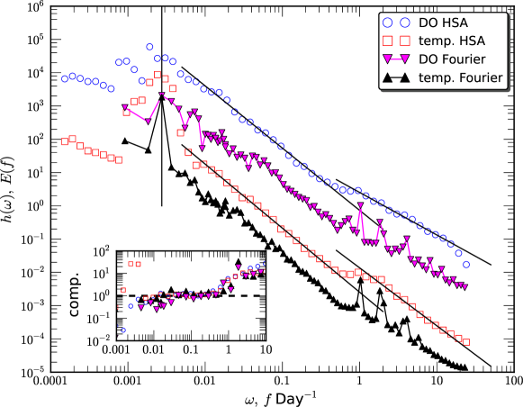
Figure 10: The Hilbert spectrum of dissolved oxygen ($\ocircle$) and temperature ($\square$), in which the vertical line indicates the annual cycle. Power law behavior is observed for both curves on the range $0.01<\omega<0.5$ day^-1 and $2<\omega<20$ day^-1, corresponding to a time scale $2<T<100$ days and $1.2<T<12$ hours, respectively. The corresponding scaling exponents are $1.93\pm 0.05$ and $1.87\pm 0.08$ for large scales, and $1.68\pm 0.10$ and $1.35\pm 0.10$ for small scales respectively. For comparison, the Fourier power spectrum is also shown for both dissolved oxygen ($\triangledown$) and temperature ($\triangle$). The inset shows the compensated spectrum $h(\omega)\omega^{2}C^{-1}$ ($E(f)f^{2}C^{-1}$) with fitted $C$ to emphasize the observed power laws.

With the IMF modes obtained from EMD algorithm, the HSA can be applied to each IMF mode. In this step, we first interpolate the IMF mode by using a Piecewise Cubic Hermite Interpolating Polynomial (phcip) algorithm into a regular time interval with $dt=30$ minutes, which is slightly larger than the mean time interval of $24$ minutes. Then the HSA is applied to extract the joint pdf $p(\mathcal{A},\omega)$. The Hilbert marginal spectrum is then calculated by using Eq. (7). Figure 10 shows the Hilbert marginal spectra for dissolved oxygen ($\ocircle$) and temperature ($\square$), in which the vertical line indicates the annual cycle. A strong annual cycle is observed for the temperature data, which is consistent with the observation of the original temperature data, see Fig. 2 b. It is emphasized here that for the temperature data with and without riding-wave around 2008, the Hilbert spectrum $h(\omega)$ are the same, showing the robustness of the present method. Power law behavior is observed on the frequency range $0.01<\omega<0.5$ day^-1, corresponding to time scales $2<T<100$ days (resp. $T=\omega^{-1}$), and $2<\omega<20$ day^-1, corresponding to time scales $1.2<T<12$ hours. The measured scaling exponents are respectively $1.93\pm 0.05$ and $1.87\pm 0.08$ for the first scaling range of temperature and dissolved oxygen, and $1.68\pm 0.10$ and $1.35\pm 0.10$ for the second scaling range. The scaling exponents for the first scaling range are statistically close to each other. For the second scaling exponent, the temperature one is close to the Kolmogorov value $5/3$ (Frisch, 1995), implying that the variation of the temperature within one day is like a passive scalar. For comparison, the corresponding Fourier power spectrum $E(f)$ is also presented. Both Hilbert and Fourier spectra show strong annual and daily cycles. However, there is no half-day cycle observed in the Hilbert spectrum. It might indicates that the half-day cycle is a harmonic from the nonlinear distortion of the daily cycle. Power law behavior is also observed for the Fourier power spectrum on the same range of time scales $2<T<100$ days as for the Hilbert framework. The corresponding scaling slope is close to $2$. To emphasize the observed power law behavior, the compensated spectra $h(\omega)\omega^{2}C^{-1}$ (resp. $E(f)f^{2}C^{-1}$) are shown in the inset. The observed plateau confirms the power law. Note that the observed $-2$ power law indicates that there might be a cascade process in the marine coastal environment (Thorpe, 2005). This should be investigated further in future studies. Let us note that a shorter portion of this data set has been studied in Zongo and Schmitt (2011): for the years 2006 to 2008, with about 50,000 data points, a Fourier analysis has found a power-law slope of $1.66$ for scales between 1 year and 2 hours, where the fit was done for this whole range; it should be noted that different fits on separated portions of the frequencies give values closer to the Hilbert-based estimates.

4.3 Time Dependent Intrinsic Correlation

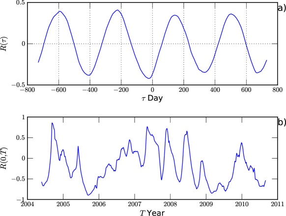
Figure 11: a) The global cross correlation coefficient $R(\tau)$ between the dissolved oxygen and the temperature. Note that there is a strong annual cycle with a phase difference of 30 days. The global correlation coefficient is $R(0)=-0.37\pm 0.10$. b) The measured cross correlation coefficient $R(0,t_{w})$ with a sliding window $t_{w}=180$ days. It shows that the relation between dissolved oxygen and temperature varies from time to time, indicating a multi-scale property of such data sets.

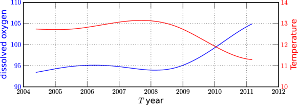
Figure 12: The trend from EMD for dissolved oxygen and temperature. The direct measurement of the cross correlation is $-0.96$, showing a global out-of-phase relation between the temperature and dissolved oxygen variation.

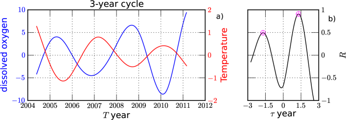
Figure 13: a) The IMF modes with a 3-year mean period. b) The measured cross correlation $R(\tau)$. They are negatively correlated with a phase difference of around 2 months. The overall correlation coefficient is $R(0)=-0.68$. The mean period is determined by the distance between the two local extrema points ($\oplus$).

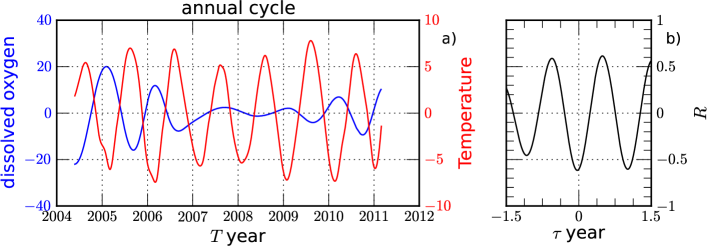
Figure 14: a) The annual cycle from EMD. b) The measured cross correlation $R(\tau)$. The overall correlation coefficient is $R(0)=-0.60$ with 14 days phase difference. Note that there is a weak period between 2007 and 2009 for both temperature and dissolved oxygen.

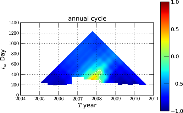
Figure 15: The measured TDIC for the annual cycle. It shows a transition from negative positive correlation between 2007 and 2008. The overall correlation coefficient is -0.60, see Fig. 14 b. The hole is the $R$ cannot pass the $t-$test. The horizontal axis is the location of the centre of the sliding window.

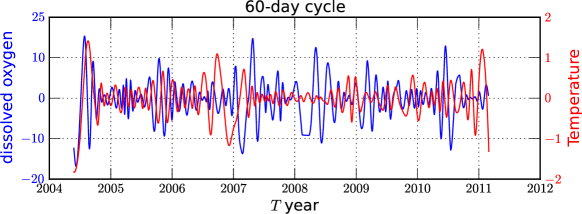
Figure 16: The 60-day cycle from EMD. The overall correlation coefficient is -0.02 with 15 days phase difference.

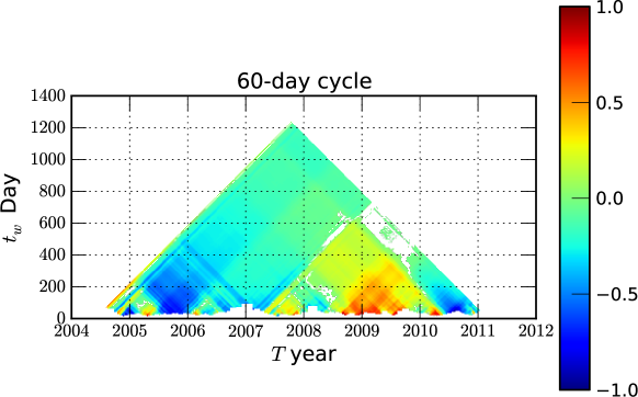
Figure 17: The measured TDIC for 60-day mean period. There is a more than half year strong correlation pattern around 2009 and 2010. The overall correlation coefficient is -0.02.

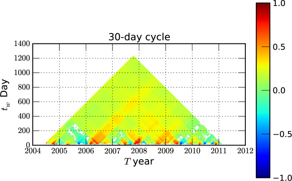
Figure 18: The measured TDIC for 30-day mean period on the range May 2004 $\sim$ January 2008. There are more than half a years strong correlation patterns between January 2006 and June 2006. The overall correlation coefficient is 0.17.

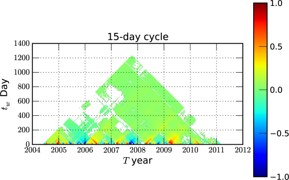
Figure 19: The measured TDIC for the 15-day mean period. The overall correlation coefficient is 0.10.

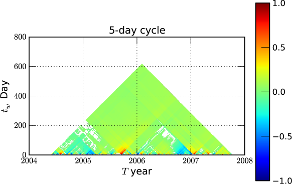
Figure 20: The measured TDIC for the 5-day mean period. The overall correlation coefficient is 0.1.

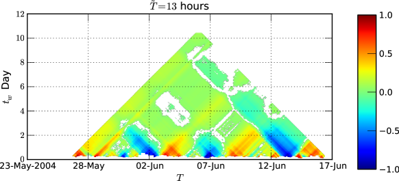
Figure 21: The measured TDIC for the 13-day mean period. The overall correlation coefficient is 0.1. The holes indicate that the measured TDIC can not pass the $t$-test.

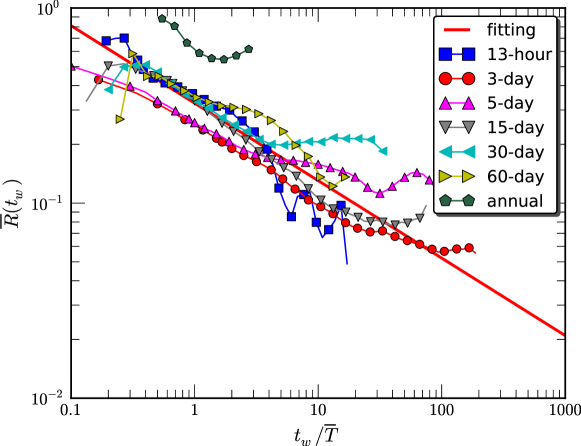
Figure 22: The measured absolute mean value $\overline{R}(t_{w})$ for different time scales $\overline{T}$. For display clarity, the sliding window $t_{w}$ is normalized by their owner mean period $\overline{T}$. Power law behavior is observed on the $0.4<t_{w}/\overline{T}<4$ with a scaling exponent $0.40\pm 0.01$.

The correlation between this two data sets is considered here. Figure 11 displays the global cross correlation $R(\tau)$ between the dissolved oxygen and the temperature. There is strong annual cycle with a 30 days phase difference. The global correlation coefficient is found to be $R(0)=-0.37\pm 0.10$. To show the variation of $R$, the cross correlation coefficient $R(0,t_{w})$ is calculated with a sliding window $t_{w}=180$ days, which is shown in Fig.11 b. The standard deviation is found to be $0.40$. Note that the standard deviation as a measurement of the stationarity has been introduced, see Eq. (10). It confirms that the global cross correlation coefficient ignores the local/multi-scale information, which could be recovered by a proper methodology (Chen et al., 2010).

After the EMD decomposition, the data sets are represented in a multi-scale way (Huang et al., 1998; Flandrin and Gonçalvès, 2004; Huang, 2009). These are used for the multi-scale correlation analysis. Time scales larger than or equal to one year are now considered. Figure 12 shows the residual from the EMD algorithm, which has been recognized as the trend of the given data (Wu et al., 2007; Moghtaderi et al., 2011). Figure 13 a) shows the IMF modes with a 3-year mean period, and Figure 13 b) the corresponding cross correlation $R(\tau)$. They show a negative correlation with each other with a phase difference of 2 months. Figure 14 a) shows the annual cycle from EMD, Figure 14 b) the corresponding cross correlation $R(\tau)$. Again they are negatively correlated with each other. The overall correlation coefficient is -0.63 with a 14 day phase difference. An interesting observation is that there is a weak period between 2007 and 2009 for both data sets, indicating that a special event has happened. The measured TDIC is shown in Figure 15. There is a positive correlation around 2008. The transition from negative (resp. out-of-phase) to positive (in-phase) and again to negative correlation from mid of 2007 to the mid of 2008 might be an effect of the warming from mid 2007 until almost 2009. During this period, the sea water temperature was consequently $2\,^{\circ}\mathrm{C}$ higher than usual in the winter time. Therefore, the out-of-phase relation between DO and temperature is affected by this event.

Let us consider scales less than one year. Figure 16 shows the IMF modes with a mean period of 60 days. They are positively correlated with each other on some portions and negatively correlated on others, showing rich dynamics. However, the overall correlation coefficient is small (resp. $-0.02$). Figure 17 displays the measured TDIC, which confirms the direct observation of the IMF modes. A strong positive correlation is observed during the time period 2009$\sim$2010. Due to the complexity of the coastal environment system, the exact reason for this changes from negative to positive is unclear. It will be addressed in future studies. For time scales smaller than 60 days, the original IMF are not shown here, but only the measured TDIC. Figure 18$\sim$21 show the measured TDIC for mean periods of 30-day to 13-hour respectively. All TDICs show rich patterns at a small sliding window. Let us also note that with the increase of the window size they decorrelate. To show the decorrelation of the TDIC, a absolute mean value of the measured $R_{i}(t_{k}^{n})$ is defined, i.e.,

$$\overline{R}(t_{w})=\langle|R(t_{k}^{n},t_{w})|\rangle_{t}$$ (13)

Figure 22 shows in a log-log plot of the measured $\overline{R}(t_{w})$ for seven time scales considered above. Note that the horizontal axis $t_{w}$ has been normalized by their mean period $\overline{T}$. Generally speaking, the curves are decreasing with the increasing of the sliding window size $t_{w}/\overline{T}$, showing the decorrelation between dissolved oxygen and temperature on different scales. A power law behavior is observed on $0.4<t_{w}/\overline{T}<4$, i.e.,

$$\overline{R}\sim(t_{w}/\overline{T})^{-\alpha}$$ (14)

with a scaling exponent $\alpha=0.40\pm 0.10$ obtained by using a least square fitting algorithm. This indicates that the considered modes decorrelate with each other in a power law way, with the same law.

5 Conclusion

Marine environmental time series can be quite complex, especially with the influence of turbulent stochastic fluctuations, multi-scale dynamics, and deterministic forcings. Such time series are as a result often non stationary and nonlinear. It has been shown elsewhere that the EMD method, together with Hilbert spectral analysis, is less influenced by deterministic forcing than other methods (Huang et al., 2010, 2011). Here this approach was applied to automatic temperature and oxygen data. Power law spectra was found using Hilbert spectral analysis. Both series have similar spectra over the range from 2 to 100 days, whereas there is a difference in slopes for high frequency power law regimes. The time evolution and scale dependence of cross correlations between both series were considered. The decomposition into modes helped to estimate how correlations vary among scales. It was found that the trends are perfectly anti-correlated, and that the modes of mean year 3 years and 1 year have also negative correlation, whereas higher frequency modes have a much smaller correlation. A new methodology was also applied, time-dependent intrinsic correlations: this showed the patterns of correlations at different scales, for different modes.

Such analysis may help to identify some key mechanisms. Here a strong anti-correlation was found for modes of mean time scale of 3 years, with a phase shift of 2 months. An explanation of such a result could be that, at these scales, higher temperatures may favour larger phytoplankton growth rate, and hence, with a time delay, a lower percentage of oxygen. Of course such relations are not always true, and the color maps of TDIC reveal the variations of the strength of such relationship.

While Fourier space methods can produce in some respects similar results for the power spectra, cross-correlations through co-spectra, and some colour maps of correlations in frequency space, they do not provide time-frequency information like the EMD based method used here. Furthermore, the TDIC tested here is a new method for correlation analysis that could be applied on other time series from the environmental and oceanic sciences, since in these fields time series are typically complex, with fluctuations at all scales, and nonlinear and non stationary features.

References

References

- Best et al. (2007) Best, M., Wither, A., Coates, S., 2007. Dissolved oxygen as a physico-chemical supporting element in the water frameworkdirective. Marine Pollution Bulletin 55, 53–64.
- Blain et al. (2004) Blain, S., Guillou, J., Treguer, P., Woerther, P., Delauney, L., Follenfant, E., Gontier, O., Hamon, M., Leilde, B., Masson, A., Tartub, C., Vuillemin, R., 2004. High frequency monitoring of the coastal environment using the marel buoy. J. Environ. Monitoring 6, 569–575.
- Chang and Dickey (2001) Chang, G., Dickey, T., 2001. Optical and physical variability on timescales from minutes to the seasonal cycle on the new england shelf: July 1996 to june 1997. J. Geophys. Res. 106, 9435–9453.
- Chavez (1997) Chavez, et al., 1997. Moorings and drifters for real-time interdisciplinary oceanography. J. Atmos. Ocean. Technol. 14, 1199–1211.
- Chen et al. (2010) Chen, X., Wu, Z., Huang, N. E., 2010. The time-dependent intrinsic correlation based on the empirical mode decomposition. Adv. Adapt. Data Anal 2, 233–265.
- Cohen (1995) Cohen, L., 1995. Time-frequency analysis. Prentice Hall PTR Englewood Cliffs, NJ.
- Coughlin and Tung (2004) Coughlin, K. T., Tung, K. K., 2004. 11-Year solar cycle in the stratosphere extracted by the empirical mode decomposition method. Adv. Space Res. 34 (2), 323–329.
- Dätig and Schlurmann (2004) Dätig, M., Schlurmann, T., 2004. Performance and limitations of the hilbert–huang transformation (hht) with an application to irregular water waves. Ocean Eng. 31 (14), 1783–1834.
- Dickey (1991) Dickey, T., 1991. The emergence of concurrent high resolution physical and bio-optical measurements in the upper ocean and their applications. Rev. Geophys. 29, 383–413.
- Dur et al. (2007) Dur, G., Schmitt, F. G., Souissi, S., 2007. Analysis of high frequency temperature time series in the seine estuary from the marel autonomous monitoring buoy. Hydrobiologia 588.
- Echeverria et al. (2001) Echeverria, J. C., Crowe, J. A., Woolfson, M. S., Hayes-Gill, B. R., 2001. Application of empirical mode decomposition to heart rate variability analysis. Med. Biol. Eng. Comput. 39 (4), 471–479.
- Flandrin (1998) Flandrin, P., 1998. Time-frequency/time-scale analysis. Academic Press.
- Flandrin and Gonçalvès (2004) Flandrin, P., Gonçalvès, P., 2004. Empirical Mode Decompositions as Data-Driven Wavelet-Like Expansions. Int. J. Wavelets, Multires. Info. Proc. 2 (4), 477–496.
- Flandrin et al. (2004) Flandrin, P., Rilling, G., Gonçalvès, P., 2004. Empirical mode decomposition as a filter bank. IEEE Sig. Proc. Lett. 11 (2), 112–114.
- Frisch (1995) Frisch, U., 1995. Turbulence: the legacy of AN Kolmogorov. Cambridge University Press.
- Garcia and Gordon (1992) Garcia, H. E., Gordon, L. I., 1992. Oxygen solubility in seawater: better fitting equations. Limnology and Oceanography 37, 1307–1312.
- Hoover (2003) Hoover, K., 2003. non-stationary time series conintegration and the principle of the common cause. British J. Philosophy Sci. 54, 527–551.
- Huang (2005) Huang, N. E., 2005. Hilbert-Huang Transform and Its Applications. World Scientific, Ch. 1. Introduction to the Hilbert-Huang transform and its related mathematical problems, pp. 1–26.
- Huang et al. (1999) Huang, N. E., Shen, Z., Long, S. R., 1999. A new view of nonlinear water waves: The Hilbert Spectrum . Annu. Rev. Fluid Mech. 31 (1), 417–457.
- Huang et al. (1998) Huang, N. E., Shen, Z., Long, S. R., Wu, M. C., Shih, H. H., Zheng, Q., Yen, N., Tung, C. C., Liu, H. H., 1998. The empirical mode decomposition and the Hilbert spectrum for nonlinear and non-stationary time series analysis. Proc. R. Soc. London, Ser. A 454 (1971), 903–995.
- Huang et al. (2009a) Huang, N. E., Wu, Z., Long, S., Arnold, K., Chen, X., Blank, K., 2009a. On instantaneous frequency. Adv. Adapt. Data Anal 1 (2), 177–229.
- Huang (2009) Huang, Y., 2009. Arbitrary-order hilbert spectral analysis: Definition and application to fully developed turbulence and environmental time series. Ph.D. thesis, Université des Sciences et Technologies de Lille - Lille 1, France & Shanghai University, China.
- Huang et al. (2010) Huang, Y., Schmitt, F., Lu, Z., Fougairolles, P., Gagne, Y., Liu, Y., 2010. Second-order structure function in fully developed turbulence. Phys. Rev. E 82 (2), 026319.
- Huang et al. (2008) Huang, Y., Schmitt, F., Lu, Z., Liu, Y., 2008. An amplitude-frequency study of turbulent scaling intermittency using hilbert spectral analysis. Europhys. Lett. 84, 40010.
- Huang et al. (2009b) Huang, Y., Schmitt, F., Lu, Z., Liu, Y., 2009b. Analysis of daily river flow fluctuations using empirical mode decomposition and arbitrary order hilbert spectral analysis. J. Hydrol. 373, 103–111.
- Huang et al. (2011) Huang, Y., Schmitt, F. G., Hermand, J.-P., Gagne, Y., Lu, Z., Liu, Y., 2011. Arbitrary-order Hilbert spectral analysis for time series possessing scaling statistics: comparison study with detrended fluctuation analysis and wavelet leaders. Phys. Rev. E 84 (1), 016208.
- Hwang et al. (2003) Hwang, P. A., Huang, N. E., Wang, D. W., 2003. A note on analyzing nonlinear and non-stationary ocean wave data. Appl. Ocean Res. 25 (4), 187–193.
- Jánosi and Müller (2005) Jánosi, I., Müller, R., 2005. Empirical mode decomposition and correlation properties of long daily ozone records. Phys. Rev. E 71 (5), 56126.
- Long et al. (1995) Long, S. R., Huang, N. E., Tung, C. C., Wu, M. L., Lin, R. Q., Mollo-Christensen, E., Yuan, Y., 1995. The Hilbert techniques: an alternate approach for non-steady time series analysis. IEEE Geoscience and Remote Sensing Soc. Lett. 3, 6–11.
- Loutridis (2004) Loutridis, S. J., 2004. Damage detection in gear systems using empirical mode decomposition. Eng. Struct. 26 (12), 1833–1841.
- Moghtaderi et al. (2011) Moghtaderi, A., Borgnat, P., Flandrin, P., 2011. Trend filtering: empirical mode decompositions versus and hodrick–prescott. Adv. Adapt. Data Anal 3 (01n02), 41–61.
- Molla et al. (2006a) Molla, M. K. I., Rahman, M. S., Sumi, A., Banik, P., 2006a. Empirical mode decomposition analysis of climate changes with special reference to rainfall data. Discrete Dyn. Nat. Soc. 2006, Article ID 45348, 17 pages, doi:10.1155/DDNS/2006/45348.
- Molla et al. (2006b) Molla, M. K. I., Sumi, A., Rahman, M. S., 2006b. Analysis of Temperature Change under Global Warming impact using Empirical Mode Decomposition . Int. J. Info. Tech. 3 (2), 131–139.
- Papadimitriou et al. (2006) Papadimitriou, S., Sun, J., Yu, P. S., 2006. Local correlation tracking in time series. Proc. Sixth Int. Conf. Date Mining, 456-465.
- Rilling et al. (2003) Rilling, G., Flandrin, P., Gonçalvès, P., 2003. On empirical mode decomposition and its algorithms. IEEE-EURASIP Workshop on Nonlinear Signal and Image Processing.
- Rodo and Rodriguez-Arias (2006) Rodo, X., Rodriguez-Arias, M. A., 2006. A new method to detect transitory signatures and local time/space variability structures in the climate system: the scale-dependent correlation analysis. Clim. Dyn. 27, 441–458.
- Schmitt et al. (2009) Schmitt, F. G., Huang, Y., Lu, Z., Liu, Y., Fernandez, N., 2009. Analysis of velocity fluctuations and their intermittency properties in the surf zone using empirical mode decomposition. J. Mar. Sys. 77, 473–481.
- Schmitt et al. (2008) Schmitt, F. G., Dur, G., Souissi, S., Brizard Zongo, S., 2008. Statistical properties of turbidity, oxygen and pH fluctuations in the Seine river estuary (France). Physica A 387 (26), 6613–6623.
- Thorpe (2005) Thorpe, S. A., 2005. The turbulent ocean. Cambridge University Press.
- Veltcheva and Soares (2004) Veltcheva, A. D., Soares, C. G., 2004. Identification of the components of wave spectra by the Hilbert Huang transform method. Appl. Ocean Res. 26 (1-2), 1–12.
- Woerther (1998) Woerther, P., 1998. Marel: Mesures automatisées en réseau pour l’environnement littoral. Léau, Les industrie, Les nuisances 217, 67–72.
- Wu and Huang (2004) Wu, Z., Huang, N. E., 2004. A study of the characteristics of white noise using the empirical mode decomposition method. Proc. R. Soc. London, Ser. A 460, 1597–1611.
- Wu et al. (2007) Wu, Z., Huang, N. E., Long, S. R., Peng, C., 2007. On the trend, detrending, and variability of nonlinear and non-stationary time series. PNAS 104 (38), 14889.
- Wu and Hunag (2009) Wu, Z., Hunag, N. E., 2009. Ensemble empirical mode decomposition: a noise-assisted data analysis method. Adv. Adapt. Data Anal. 1, 1–41.
- Zhu et al. (1997) Zhu, X., Shen, Z., Eckermann, S. D., Bittner, M., Hirota, I., Yee, J. H., 1997. Gravity wave characteristics in the middle atmosphere derived from the empirical mode decomposition method. J. Geophys. Res 102, 16545–16561.
- Zongo et al. (2011) Zongo, S., Schmitt, F., Lefebvre, A., 2011. Observations biogéochimiques des eaux côtières à boulogne-sur-mer à haute fréquence: les measures automatiques de la bouée marel,. in Du naturalisme à l’écologie, edité par F.G. Schmitt, Presses de lÚOF, 253–266.
- Zongo and Schmitt (2011) Zongo, S. B., Schmitt, F. G., 2011. Scaling properties of pH fluctuations in coastal waters of the english channel: pH as a turbulent active scalars. Nonlinear Processes in Geophysics 18, 829–839.