Non-standard discretization of biological models

Abstract

We consider certain types of discretization schemes for differential equations with quadratic nonlinearities, which were introduced by Kahan, and considered in a broader setting by Mickens. These methods have the property that they preserve important structural features of the original systems, such as the behaviour of solutions near to fixed points, and also, where appropriate (e.g. for certain mechanical systems), the property of being volume-preserving, or preserving a symplectic/Poisson structure. Here we focus on the application of Kahan’s method to models of biological systems, in particular to reaction kinetics governed by the Law of Mass Action, and present a general approach to birational discretization, which is applied to population dynamics of Lotka-Volterra type.

1 Introduction

In 1993 Kahan gave a set of lectures entitled “Unconventional numerical methods for trajectory calculations,” in which he proposed a method for discretizing a set of differential equations

$$\dot{\bf x}={\bf f}({\bf x}),$$ (1)

where all the components of the vector field ${\bf f}$ are polynomial functions of degree at most two in the components $x_{1},x_{2},\ldots,x_{N}$ of the vector ${\bf x}$, and the dot denotes the time derivative $\mathrm{d}/\mathrm{d}t$. Kahan’s method consists of replacing the left hand side of (1) by the standard forward difference, while on the right hand side quadratic, linear and constant terms are replaced according to a symmetric rule, so that overall the method is specified as follows:

$$\dot{x}_{i}\to\frac{\tilde{x}_{i}-x_{i}}{h},\quad x_{i}x_{j}\to\frac{x_{i}\tilde{x}_{j}+\tilde{x}_{i}x_{j}}{2},\quad x_{i}\to\frac{x_{i}+\tilde{x}_{i}}{2},\quad c\to c.$$ (2)

Above and throughout we use the tilde to denote the finite difference approximation to a dependent variable shifted by a time step $h$, i.e. $x_{i}(t+h)\approx\tilde{x}_{i}$.

The replacements (2) result in a difference equation of the form

$$\frac{\tilde{{\bf x}}-{\bf x}}{h}={\bf Q}({\bf x},\tilde{{\bf x}}),$$ (3)

where the right hand side is a vector function of degree two. Thus it appears to be an implicit scheme, in the sense that (3) defines $\tilde{{\bf x}}$ implicitly as a function of ${\bf x}$. However, the fact that the formulae (2) are linear in each of the variables $\tilde{x}_{i}$ and $x_{j}$ means that (3) can be solved explicitly to find $\tilde{{\bf x}}$ as a rational function of ${\bf x}$, and vice versa, yielding a birational map $\varphi:{\bf x}\mapsto\tilde{{\bf x}}$. As shown in [8], the map can be written explicitly as

$$\varphi:\quad\tilde{{\bf x}}={\bf x}+h\left({\bf I}-\frac{h}{2}{\bf f}^{\prime}({\bf x})\right)^{-1}{\bf f}({\bf x}),$$ (4)

where ${\bf I}$ denotes the $N\times N$ identity matrix, and ${\bf f}^{\prime}$ is the Jacobian of ${\bf f}$, while the inverse is

$$\varphi^{-1}:\quad{{\bf x}}=\tilde{{\bf x}}-h\left({\bf I}+\frac{h}{2}{\bf f}^{\prime}(\tilde{{\bf x}})\right)^{-1}{\bf f}(\tilde{{\bf x}}).$$ (5)

The above method is second-order, but Kahan and Li showed how it can be used with suitable composition schemes to generate methods of higher order [8, 9].

Roegers proved that (in contrast to Euler’s method) Kahan’s method preserves the local stability of steady states of (1). Indeed, the steady states ${\bf x}^{*}$ of the differential system, satisfying ${\bf f}({\bf x}^{*})=0$, coincide with those of (4), i.e. the solutions of $\varphi({\bf x}^{*})={\bf x}^{*}$, and taking the derivative of $\varphi$ at such an ${\bf x}^{*}$ gives

$$\varphi^{\prime}({\bf x}^{*})={\bf I}+h\left({\bf I}-\frac{h}{2}{\bf f}^{\prime}({\bf x}^{*})\right)^{-1}{\bf f}^{\prime}({\bf x}^{*}).$$

Hence to each eigenvalue ${\lambda}$ of ${\bf f}^{\prime}$ at ${\bf x}^{*}$ there corresponds an eigenvalue $\mu(h)$ of $\varphi^{\prime}$ at ${\bf x}^{*}$, with the same eigenvector, where

$$\mu(h)=\frac{1+\frac{h{\lambda}}{2}}{1-\frac{h{\lambda}}{2}}.$$ (6)

The above transformation sends the region Re$\,{\lambda}<0$ to $|\mu(h)|<1$, which identifies asymptotically stable directions at steady states of (1) with those for (4), and similarly for unstable directions (Re$\,{\lambda}>0$ is sent to $|\mu(h)|>1$). These local stability properties go some way towards explaining why Kahan’s method seems to preserve global structural features of solutions of (1).

In the context of Hamiltonian mechanics, Hirota and Kimura rediscovered Kahan’s prescription (2) as a new method to discretize Euler’s equations for a top spinning about a fixed point [4]. This stimulated further interest in the method, and as a result many new completely integrable symplectic/Poisson maps were found (see [5], for instance). Despite an extensive survey of algebraically completely integrable discrete systems obtained via Kahan’s method [14], the general conditions under which a quadratic Hamiltonian vector field (1) produces a map (4) that preserves a symplectic (or Poisson) structure, as well as one or more first integrals, are still unknown. Nevertheless, considerable progress was made recently by Celledoni et al. [2], who showed that Kahan’s method is perhaps not as “unconventional” as originally thought, since it coincides with the Runge-Kutta method

$$\frac{\tilde{{\bf x}}-{\bf x}}{h}=-\frac{1}{2}{\bf f}({\bf x})+2{\bf f}\left(\frac{{\bf x}+\tilde{{\bf x}}}{2}\right)-\frac{1}{2}{\bf f}(\tilde{{\bf x}})$$

applied to quadratic vector fields ${\bf f}$. Moreover, if (1) is a Hamiltonian system with a constant Poisson structure and a cubic Hamiltonian function, then the corresponding map (4) has a rational first integral and preserves a volume form (Propositions 3,4 and 5 in [2]).

Rather than applications in mechanics, in this paper we focus on some applications of Kahan’s method to biological models. In the next section we discuss how this method is well suited to modelling reaction kinetics. The basic enzyme reaction is used as an example to illustrate the method, and we see how the discretization reproduces the transient behaviour inherent in this system.

Mickens proposed a broad non-standard approach to preserving structural features of differential equations under discretization [10], which has been applied to many different problems (as reviewed by Patidar in [13]). In the third section we consider population dynamics, and more specifically the Lotka-Volterra model for a predator-prey interaction. This was one of the examples originally treated by Kahan in applying his symmetric method, but Mickens found an asymmetric discrete Lotka-Volterra system with the same qualitative features [11]. Here we give the details of a general method, first sketched in [6], to obtain non-standard discretizations by requiring that the resulting maps should be birational. As an application of the method, a classification of birational discrete Lotka-Volterra systems is derived, and this is then used to reproduce some results of Roeger on symplectic Lotka-Volterra maps [17].

The final section is devoted to some conclusions.

2 Discrete reaction kinetics: the basic enzyme reaction

Systems of differential equations of the form (1), with ${\bf f}$ being a quadratic vector field, are ubiquitous in chemistry, and in biochemistry in particular. They arise immediately from reaction kinetics involving reactions of the form $A+B\mathop{\rightarrow}C$, $A\mathop{\rightarrow}B+C$, or $A+B\mathop{\rightarrow}C+D$, where $A,B,C,D$ represent different molecular species. In that case, the Law of Mass Action implies that the rate of change of concentration of each reactant is given by a sum of linear and quadratric terms in the concentrations. Processes involving collisions of three or more molecules are statistically rare, and although trimolecular reactions may be observed empirically, it is usually understood that in practice they are mediated by dimolecular reactions (which may take place very rapidly). Thus quadratic nonlinearities are the norm in reaction kinetics.

Kahan’s discretization method is well-suited to reaction kinetics models, where the variables $x_{i}$, $x_{j}$ in (2) would represent concentrations of different chemical species. From a practical point of view, the only potential difficuly is with inverting the matrix ${\bf I}-\frac{h}{2}{\bf f}^{\prime}({\bf x})$ on the right hand side of (4), which becomes unfeasible to do algebraically when $N$ (the number of species) is large. However, viewed numerically for a given value of ${\bf x}$ and a small $h$, this matrix is a small perturbation of the identity, and its inverse can be expanded as a geometric series,

$$\Big{(}{\bf I}-\frac{h}{2}{\bf f}^{\prime}\Big{)}^{-1}={\bf I}+\frac{h}{2}{\bf f}^{\prime}+\frac{h^{2}}{4}({\bf f}^{\prime})^{2}+\frac{h^{3}}{8}({\bf f}^{\prime})^{3}+\ldots,$$

and then truncated at a suitable power of $h$ if necessary. Moreover, if each species in the reaction network is only coupled to a small number of others then the matrix will be sparse, and there are efficient algorithms for inverting matrices of this kind.

To illustrate how Kahan’s method works in reaction kinetics, we consider the basic enzyme reaction, which is given by

$$S+E\mathop{\rightleftarrows}^{k_{1}}_{k_{-1}}C,\qquad C\mathop{\longrightarrow}^{k_{2}}E+P,$$

where $S$ is the substrate, $E$ is the enzyme, $C$ is a combined substrate-enzyme complex, $P$ is the product and $k_{-1},k_{1},k_{2}$ are rate constants. Our presentation follows that of chapter 6 in [12] very closely.

From the above reaction scheme, the Law of Mass Action yields a system of four differential equations which describe the rate of change of concentration of each reactant, as follows:

$$\begin{array}[]{rclrcl}\dot{s}&=&-k_{1}es+k_{-1}c,&\dot{e}&=&-k_{1}es+(k_{-1}+k_{2})c,\\ \dot{c}&=&k_{1}es-(k_{-1}+k_{2})c,&\dot{p}&=&k_{2}c.\end{array}$$ (7)

The lower case letters $s,e,c,p$ are used to denote the concentrations of the reactants $S,E,C,P$, respectively. For an enzyme reaction, we can assume that initially none of the enzyme has bound with the substrate, and no product has yet formed, so that the initial conditions take the form

$$s(0)=s_{0},\qquad e(0)=e_{0},\qquad c(0)=0=p(0).$$ (8)

The right hand side of the system (7) has degree two overall, which means that Kahan’s method (2) can be applied immediately, to produce the discretization

$$\begin{array}[]{rcl}(\tilde{s}-s)/h&=&-k_{1}(e\tilde{s}+\tilde{e}s)/2+k_{-1}(c+\tilde{c})/2,\\ (\tilde{e}-e)/h&=&-k_{1}(e\tilde{s}+\tilde{e}s)/2+(k_{-1}+k_{2})(c+\tilde{c})/2,\\ (\tilde{c}-c)/h&=&k_{1}(e\tilde{s}+\tilde{e}s)/2-(k_{-1}+k_{2})(c+\tilde{c})/2,\\ (\tilde{p}-p)/h&=&k_{2}(c+\tilde{c})/2.\end{array}$$ (9)

However, rather than go ahead and solve the discrete system explicitly for $\tilde{s},\tilde{e},\tilde{c},\tilde{p}$, we will use a special feature of the enzyme reaction in order to simplify the problem.

The essential feature of an enzyme is that it is a catalyst, so that it is not changed overall by the reactions it is involved in. This means that the total amount of enzyme in the system (free enzyme in the form of $E$, and enzyme bound into the complex $C$) must be conserved with time. From (7) this can be seen directly in the form of the conservation law

$$\dot{e}+\dot{c}=0\qquad\Rightarrow\qquad e(t)+c(t)=\mathrm{constant}=e_{0},\qquad\forall t\geq 0,$$

where the initial conditions (8) are used to specify the value of the first integral $e+c$.

$\begin{array}[]{cc}{\includegraphics[width=158.99377pt]{xyplot.jpg}}&{\includegraphics[width=158.99377pt]{zplot.jpg}}\end{array}$

Figure 1: Plots of $x$ and $y$ against $t$ (left) and $z$ (right) against $t$ from numerical integration of (10) using Kahan’s method with $\nu=0.6$, $\mu=0.5$, $\varepsilon=10^{-2}$, $h=10^{-3}$.

The fact that the linear function $e+c$ is conserved means that $e$ (or $c$) can be eliminated from the system (7), so that the problem is reduced to solving a three-dimensional system. As noted in [2], the properties of Kahan’s method mean that it preserves linear first integrals, and so, as is clear from the above equations, the discrete system (9) has the same first integral:

$$\tilde{e}+\tilde{c}=e+c.$$

Thus we can also set $e=e_{0}-c$ to eliminate $e$ from (9), and then solve the resulting three-dimensional discrete system. Rather than doing so immediately, it is helpful to rescale all the variables in (7), so that (after eliminating $e$) everything is written in terms of dimensionless quantities $x,y,z$ and $\tau$, where

$$x=\frac{s}{s_{0}},\qquad y=\frac{c}{e_{0}},\qquad z=\frac{p}{s_{0}},\qquad\tau=k_{1}e_{0}t.$$

Then the dimensionless system is

$$\begin{array}[]{rcl}\dot{x}&=&-x+\mu y+xy,\\ \varepsilon\dot{y}&=&x-\nu y-xy,\\ \dot{z}&=&(\nu-\mu)y,\end{array}$$ (10)

where now the dot denotes $\mathrm{d}/\mathrm{d}\tau$, and the dimensionless parameters are

$$\mu=\frac{k_{-1}}{k_{1}s_{0}},\qquad\nu=\frac{k_{-1}+k_{2}}{k_{1}s_{0}},\qquad\varepsilon=\frac{e_{0}}{s_{0}}.$$

From (8), the initial conditions for (10) are

$$x(0)=1,\qquad y(0)=0=z(0).$$ (11)

Typically, the amount of enzyme is very small compared with the concentrations of the other reactants, so the parameter $\varepsilon$ should be small. According to Murray [12], the realistic range is $10^{-7}\leq\varepsilon\leq 10^{-2}$.

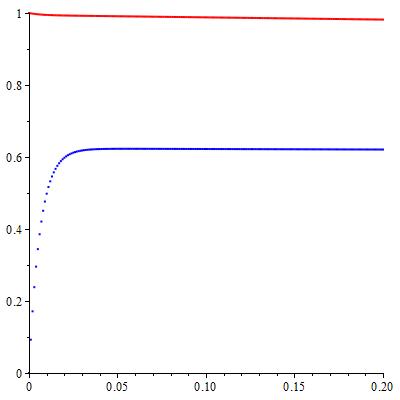
Figure 2: As for Figure 1, with details of $x$ (above) and $y$ (below) against $t$ for $0\leq t\leq 0.2$.

In terms of the dimensionless variables, Kahan’s method applied to (10) yields the discrete three-dimensional system

$$\begin{array}[]{rcl}2(\tilde{x}-x)/h&=&-(x+\tilde{x})+\mu(y+\tilde{y})+x\tilde{y}+\tilde{x}y,\\ 2\varepsilon(\tilde{y}-y)/h&=&x+\tilde{x}-\nu(y+\tilde{y})-x\tilde{y}-\tilde{x}y,\\ 2(\tilde{z}-z)/h&=&(\nu-\mu)(y+\tilde{y}).\end{array}$$ (12)

Using the formula (4) to solve for the shifted variables, the resulting map can be written in matrix form as

$$\left(\begin{array}[]{c}\tilde{x}\\ \tilde{y}\\ \tilde{z}\end{array}\right)=\left(\begin{array}[]{c}x\\ y\\ z\end{array}\right)+h\,\left(\begin{array}[]{ccc}1+\frac{h}{2}(1-y)&-\frac{h}{2}(\mu+x)&0\\ -\frac{h}{2\varepsilon}(1-y)&1+\frac{h}{2\varepsilon}(\nu+x)&0\\ 0&-\frac{h}{2}(\nu-\mu)&1\end{array}\right)^{-1}\left(\begin{array}[]{c}-x+\mu y+xy\\ \varepsilon^{-1}(x-\nu y-xy)\\ (\nu-\mu)y\end{array}\right).$$

In practice, since the equations for $x$ and $y$ decouple from $z$, the dimensionless concentration of the product, it convenient to solve for $x$ and $y$ first, and then the value $z_{n}$ (the value of $z$ after $n$ steps, which approximates $z(nh)$) is given by

$$z_{n}=\frac{h}{2}(\nu-\mu)\sum_{i=0}^{n-1}(y_{i}+y_{i+1}),$$

which follows from the third equation in (12) and the initial conditions (11).

Some numerical results obtained by applying the discretization (12) are shown in Figure 1. There are a few things worthy of comment here. Note that the value of the time step $h$ has been chosen to be an order of magnitude smaller than the small parameter $\varepsilon$. There is also an apparently anomalous feature of the left hand plot: the solution curve for $x$ starts with $x=1$ at time zero, as it should according to the initial values (11); but the value of $y$ appears to start at $y\approx 0.6$, when it should start with $y=0$. Subsequently the values of $x$ and $y$ both tend asymptotically towards zero; that is to be expected, since the decoupled system for $x$ and $y$, given by the first two equations in (10), has a steady state at $(x,y)=(0,0)$ which is stable and unique, and the results of [15], based on the formula (6), imply that the discrete system has the same local stability. From the plot on the right hand side of Figure 1, it is seen that the amount of product in the reaction, measured by the variable $z$, tends to an equilibrium value (proportional to the area under the graph of $y$).

The anomalous aspect of Figure 1, namely the initial behaviour of $y$, can be understood by looking in detail at the value of $y$ for very small times. This is shown in Figure 2, from which it can be seen that in fact the value of $y$ undergoes an early transient phase of very rapid expansion from the initial value $y=0$, before reaching a value around 0.6 and then starting to decay. The reason for this rapid change is the presence of the parameter $\varepsilon\ll 1$ in the equation for $y$. If the left hand side of the second equation in (10) is ignored, then the Michaelis-Menten approximation

$$y\approx\frac{x}{\nu+x}$$

results, and putting in $\nu=0.6$ and $x=1$ gives the “initial” value $y=0.625$. The initial expansion in $y$ takes place over a timescale of the order of $\varepsilon$. A fuller understanding of the solution can be achieved by using matched asymptotic expansions, taking one type of asymptotic series solution close to time zero (the inner solution), and another for larger times (the outer solution); more details can be found in [12]. The low resolution of the first part of the plot of $y$ in Figure 2 indicates that a smaller time step $h$ is required for the integration at very early times, in order to obtain a more accurate picture of the inner solution.

3 Birational discretization: Lotka-Volterra systems

The classic Lotka-Volterra model for a predator-prey interaction takes the form

$$\begin{array}[]{rcl}\dot{x}&=&{\alpha}x-{\beta}xy,\\ \dot{y}&=&-{\gamma}y+{\delta}xy,\end{array}$$ (13)

where $x$ and $y$ denote the sizes of the prey and predator populations, respectively, and the parameters ${\alpha},{\beta},{\gamma},{\delta}$ are all positive. With different choices of signs for these four parameters, the system can model different types of two-species interaction (e.g. competition or mutualism), but once the signs are fixed then $x,y$ and the time $t$ can all be rescaled to obtain a dimensionless model with only a single parameter remaining (the other three being set to the value 1).

In this section we consider discretizations obtained by replacing the $x$, $y$ and $xy$ terms appearing in (13) by expressions of the general form

$$x\to ax+\hat{a}\tilde{x},\qquad y\to Ay+\hat{A}\tilde{y},\qquad xy\to bxy+c\tilde{x}\tilde{y}+dx\tilde{y}+e\tilde{x}y.$$

The results in Theorems 1 and 2 below hold true independent of the choice of parameters; so henceforth, for convenience, we consider the system with all parameters set to 1, viz

$$\begin{array}[]{ccl}\dot{x}&=&x(1-y),\\ \dot{y}&=&y(x-1).\end{array}$$ (14)

The Lotka-Volterra system (14) has a first integral given by

$$H=\log(xy)-x-y.$$ (15)

This can be viewed as a Hamiltonian function, and the system can be given an interpretation in terms of a particle moving in one dimension with position $q$ and momentum $p$, by setting

$$q=\log x,\qquad p=\log y.$$

Then expressing the Hamiltonian (15) as a function of $q$ and $p$ gives $H=q+p-e^{q}-e^{p}$, and the equations (14) can be rewritten in the form of a canonical Hamiltonian system:

$$\dot{q}=\frac{\partial H}{\partial p},\qquad\dot{p}=-\frac{\partial H}{\partial q}.$$

It follows that the flow of (14) is area-preserving in the $(q,p)$ plane, which means that (in terms of the original variables $x$ and $y$) the two-form

$${\omega}=\frac{1}{xy}\,\mathrm{d}x\wedge\mathrm{d}y$$ (16)

is preserved by this flow. The trajectories of solutions in the positive quadrant of the $(x,y)$ plane are closed curves around the steady state at $(1,1)$, which are level curves $H=$constant.

The Lotka-Volterra model was one of the examples originally considered by Kahan in his unpublished lectures from 1993. Kahan’s method applied to (14) yields

$$\begin{array}[]{ccl}(\tilde{x}-x)/{h}&=&\frac{1}{2}\Big{(}\tilde{x}+x-(\tilde{x}y+x\tilde{y})\Big{)},\\ (\tilde{y}-y)/{h}&=&\frac{1}{2}\Big{(}\tilde{x}y+x\tilde{y}-(\tilde{y}+y)\Big{)}.\end{array}$$ (17)

As shown by Sanz-Serna [18], the birational map $\varphi:(x,y)\mapsto(\tilde{x},\tilde{y})$ defined by (17) is symplectic, preserving the same two-form (16) as the original continuous system (14).

Mickens proposed a broad approach to discretization of nonlinear systems, with the aim of preserving structural properties of the solutions [10]. In [11] he presented a particular discrete predator-prey system, given by

$$\begin{array}[]{ccl}(\tilde{x}-x)/{h}&=&2x-\tilde{x}-\tilde{x}y,\\ (\tilde{y}-y)/{h}&=&-\tilde{y}+2\tilde{x}y-\tilde{x}\tilde{y}.\end{array}$$ (18)

This gives another explicit birational map of the plane: despite the fact that the overall system is not linear in $\tilde{x},\tilde{y}$, the first equation can be solved for $\tilde{x}$ and this can be substituted into the second equation to obtain a rational expression for $\tilde{y}$ in terms of $x$ and $y$. (In fact, Mickens uses a general function $\phi(h)$ in place of $h$ in the denominator on the left hand side, but since $\phi(h)=h+o(h)$ this makes no difference when $h$ is small.) Numerical studies indicate that, for small $h$, the discrete system defined by (18) also has closed orbits around $(1,1)$. The map of the $(x,y)$ plane defined by (18) preserves the same symplectic form (16) as before, which suggests why its stability properties appear to be the same as for the discretization (17).

For any system of polynomial differential equations (which need not necessarily be a quadratic one), one can try to implement Mickens’ approach in the most general way, by replacing each monomial $x_{i}x_{j}\ldots x_{k}$ with a linear combination of all possible products of the same variables with/without shifts. In [6] this was done for an example of a cubic vector field, but here we illustrate this idea by applying it to (14), which gives the general discrete system

$$\begin{array}[]{ccl}(\tilde{x}-x)/{h}&=&ax+\hat{a}\tilde{x}-(bxy+c\tilde{x}\tilde{y}+dx\tilde{y}+e\tilde{x}y),\\ (\tilde{y}-y)/{h}&=&-Ay-\hat{A}\tilde{y}+(Bxy+C\tilde{x}\tilde{y}+Dx\tilde{y}+E\tilde{x}y).\end{array}$$ (19)

In order for this to be a first-order method for (14), the coefficients are required to satisfy the constraints

$$a+\hat{a}=A+\hat{A}=b+c+d+e=B+C+D+E=1,$$ (20)

and it is further assumed that they are all independent of $h$. Thus from the start we can say that (in addition to the time step $h$) the discrete system (19) depends on 8 constant parameters $a,b,c,d,A,B,C,D$, with $\hat{a},\hat{A},e,E$ being fixed according to (20). However, for what follows it will be convenient to specify a system of the form (19) by a list of 10 parameters, viz

$$\{a,b,c,d,e,A,B,C,D,E\},$$

where it is understood that the conditions (20) hold, so only 8 of these 10 parameters are independent. So for example, Kahan’s method produces the system (17), which is specified by $\{{\frac{1}{2}},{\frac{1}{2}},0,0,{\frac{1}{2}},{\frac{1}{2}},{\frac{1}{2}},0,0,{\frac{1}{2}},{\frac{1}{2}}\}$, while Mickens’ system (18) is specified by $\{2,0,0,0,1,0,0,-1,0,2\}$.

$\begin{array}[]{cc}{\includegraphics[width=158.99377pt]{xsymp.jpg}}&{\includegraphics[width=158.99377pt]{ysymp.jpg}}\end{array}$

Figure 3: Plots of $x$ (left) and $y$ (right) against $t$ from numerical integration of (14) using the method (19) with parameters $\{{\frac{1}{2}},0,\frac{3}{2},-{\frac{1}{2}},0,{\frac{1}{2}},\frac{4}{5},0,\frac{1}{5},0\}$ and $h=0.01$.

The additional requirement that we impose is that the system (19) should give a birational map, so that $\tilde{x}$ and $\tilde{y}$ can be found explicitly and uniquely in terms of $x$ and $y$, and vice versa. Our main result can then be stated as follows.

Theorem 3.1

The system (19) is a birational discrete Lotka-Volterra equation if and only if the parameters belong to one of the following cases:

$$\begin{array}[]{clcl}\mathrm{(i)}&\{a,0,0,d,e,A,0,0,D,E\}&with&d+e=1=D+E;\\ \mathrm{(ii)}&\{a,0,0,1,0,A,B,0,D,E\}&with&B+D+E=1;\\ \mathrm{(iii)}&\{a,0,0,0,1,A,0,C,D,E\}&with&C+D+E=1;\\ \mathrm{(iv)}&\{a,b,0,d,e,A,0,0,0,1\}&with&b+d+e=1;\\ \mathrm{(v)}&\{a,0,c,d,e,A,0,0,1,0\}&with&c+d+e=1;\\ \mathrm{(vi)}&\{a,0,c,d,0,A,B,0,D,0\}&with&c+d=1=B+D;\\ \mathrm{(vii)}&\{a,b,0,0,e,A,0,C,0,E\}&with&b+e=1=C+E.\end{array}$$

In order to obtain the above list of parameter choices, in the subsequent subsections we proceed to present two different methods for finding birational discretizations, the first of which is a general method that is applicable to arbitrary vector fields, while the second is specific to the quadratic nature of the vector field (14).

3.1 The elimination method

The first method is to perform successive elimination of variables from the system (19), and then impose conditions on the polynomials which result. Let us begin by choosing to eliminate $\tilde{x}$. In the example at hand, both equations in (19) are linear in $\tilde{x}$, so we can solve either one explicitly for this variable and substitute it into the other equation, to get a polynomial relation between the remaining variables $x,y,\tilde{y}$. More generally, if the degree of nonlinearity in $\tilde{x}$ were higher, then it would be necessary to eliminate this variable from a pair of equations by taking a resultant, and for a system in dimension $N$ one should take $N-1$ resultants to eliminate one of the variables and obtain $N-1$ relations between the remaining variables. In this example, the relation found by eliminating $\tilde{x}$ has the form of a quadratic in $\tilde{y}$, that is

$$p_{2}(x,y)\tilde{y}^{2}+p_{1}(x,y)\tilde{y}+p_{0}(x,y)=0,$$ (21)

where the coefficients $p_{j}$ are all polynomials in $x$ and $y$.

One obvious way to obtain $\tilde{y}$ as a rational function of $x$ and $y$ is to require that $p_{2}$ in (21) vanishes, in which case (provided $p_{1}\neq 0$) $\tilde{y}=-p_{0}(x,y)/p_{1}(x,y)$. To be precise, up to overall scaling we have

$$p_{2}=(cD-dC)hx+c(Ah-1-h)=0\Rightarrow cD-dC=0=c(Ah-1-h),$$

since all coefficients of $p_{2}$ must vanish. The second condition above requires that $c=0$ (since $A$ is assumed independent of $h$), and then the first condition implies $dC=0$, and so we have

$$c=0\qquad\mathrm{and}\,\,\mathrm{either}\quad d=0\quad\mathrm{or}\quad C=0.$$ (22)

These conditions are sufficient to ensure that $\tilde{y}$, and hence also $\tilde{x}$ (which can be found in terms of $x,y$ and $\tilde{y}$ by solving a linear equation), are rational functions of $x$ and $y$. Thus we have a rational map $\varphi:(x,y)\mapsto(\tilde{x},\tilde{y})$ .

In order for the inverse map $\varphi^{-1}$ to be rational, we require sufficient conditions for $x$ and $y$ to be given as rational functions of $\tilde{x}$ and $\tilde{y}$. To do this, we choose to eliminate $x$ from the system (19), to obtain a quadratic in $y$, of the form

$$\tilde{p}_{2}(\tilde{x},\tilde{y}){y}^{2}+\tilde{p}_{1}(\tilde{x},\tilde{y}){y}+\tilde{p}_{0}(\tilde{x},\tilde{y})=0,$$ (23)

where, up to scaling,

$$\tilde{p}_{2}=\Big{(}B(1-c-d)-b(1-C-D)\Big{)}h\tilde{x}+b(Ah-1),$$ (24)

and we have chosen to remove $e$ and $E$ from the formulae by using the constraints (20). Now we can obtain the rational expression $y=-\tilde{p}_{0}(\tilde{x},\tilde{y})/\tilde{p}_{1}(\tilde{x},\tilde{y})$ by requiring that $\tilde{p}_{2}=0$; from (24) this gives $b=0$, because $Ah-1=0$ is not possible, and then we have

$$b=0\qquad\mathrm{and}\,\,\mathrm{either}\quad c+d=1\quad\mathrm{or}\quad B=0.$$ (25)

If these conditions hold, then $y$ is a rational function of $\tilde{x}$ and $\tilde{y}$, and hence also $x$ is.

Overall we see that requiring both sets of conditions (22) and (25) to hold is sufficient for the map $\varphi$ to be birational. This leads to three possibilities, which are the cases (i),(ii) and (iii) in Theorem 1. However, other cases are possible if we choose to eliminate the variables in a different order. So for instance, eliminating $\tilde{y}$ first gives a quadratic in $\tilde{x}$, and then requiring the leading coefficient to vanish implies that $\tilde{x}$ as a rational function of $x$ and $y$, so $\tilde{y}$ is also; and if $y$ is eliminated next and the leading coefficient of the resulting quadratic in $x$ is required to vanish, then a different set of sufficient conditions for $\varphi$ to be birational are found. These conditions lead to three different possibilities, namely case (i) (again), and cases (iv) and (v). Similarly, one can perform the elimination of $\tilde{x}$ together with $y$, or $\tilde{y}$ together with $x$; each of these options lead to four possibilities, but overall only two new cases arise in this way, namely (vi) and (vii).

An alternative way to obtain cases (i)-(vii) above is presented in the next subsection, but before proceeding with this we make some general observations about the result. Each of the discrete Lotka-Volterra equations specified in Theorem 1 depends on four arbitrary parameters (as well as the time step $h$); the choice of parameters $a$ and $A$ is arbitrary in every case. Furthermore, although they are independent cases, some of them are related to each other by inversion. To see this, observe that the inverse of any discretization method (19) is obtained by switching the roles of the dependent variables: $(x,y)\leftrightarrow(\tilde{x},\tilde{y})$. Performing this switch results in another method of the same form but with the parameters and time step changed as follows:

$$h\to-h,\quad a\to 1-a,\quad A\to 1-A,\quad b\leftrightarrow c,\quad B\leftrightarrow C,\quad d\leftrightarrow e,\quad D\leftrightarrow E.$$

From this transformation of the coefficients, it is clear that the inverse of a case (i) method is another case (i) method, and similarly the other methods are related to one another by such a transformation, so that overall the relationships between the different cases under inversion can be summarized by

$$\mathrm{(i)}\leftrightarrow\mathrm{(i)},\qquad\mathrm{(ii)}\leftrightarrow\mathrm{(iii)},\qquad\mathrm{(iv)}\leftrightarrow\mathrm{(v)},\qquad\mathrm{(vi)}\leftrightarrow\mathrm{(vii)}.\qquad$$

An example of numerical integration of (14) using one of these birational methods, namely a particular instance of case (vi), is shown in Figure 3. Observe that the graphs appear to show $x$ and $y$ varying periodically with time $t$. This is consistent with the solutions of (14) in the positive $(x,y)$ plane, which lie on closed curves corresponding to periodic orbits around the centre at $(1,1)$.

3.2 Discriminant conditions and symplectic discretizations

The elimination method presented above provided sufficient conditions for the map $\varphi$ to be birational, and by trying each possible pair of eliminations we obtained all seven cases in Theorem 1. However, there is a second way to obtain these conditions, which gives a stronger result. In order to be sure that these choices of coefficients are necessary and sufficient, we need to consider the elimination process in more detail.

Observe that, after eliminating $\tilde{x}$ to find (21), it is not strictly necessary that $p_{2}=0$, but merely that the quadratic has only rational roots. For example, case (iv) does not arise by setting $p_{2}=0=\tilde{p}_{2}$, and yet the quadratic (21) must have one rational root corresponding to the formula for $\tilde{y}$ obtained from $\varphi$ in this case. One possibility would be to set $p_{0}=0$, so that the quadratic factorizes as

$$\tilde{y}\,\Big{(}p_{2}(x,y)\tilde{y}+p_{1}(x,y)\Big{)}=0,$$

with a spurious root $\tilde{y}=0$ that can be neglected. However, we can check that setting $p_{0}=0$ and then, after eliminating $x$, either $\tilde{p}_{2}=0$ or $\tilde{p}_{0}=0$ does not lead to any consistent solutions. Thus we should consider the more general possibility that (21) has two rational roots, one of which is spurious, while the other correpsonds to the rational formula for $\tilde{y}$ which is one component of the map $\varphi$. This possibility arises if and only if the discriminant

$$\Delta(x,y)=p_{1}(x,y)^{2}-4p_{2}(x,y)p_{0}(x,y)$$

is a perfect square. Similarly, eliminating $x$ gives the quadratic (23) in $y$, and the roots are rational if and only if the corresponding discriminant $\tilde{\Delta}(\tilde{x},\tilde{y})$ is a perfect square. Imposing this condition on the two discriminants $\Delta$ and $\tilde{\Delta}$ yields a set of algebraic conditions on the parameters in (19) (omitted here for brevity); then only the cases (i)-(vii) listed in Theorem 1 are possible, and this completes the proof of the theorem without needing to consider any other eliminations.

$\begin{array}[]{cc}{\includegraphics[width=158.99377pt]{ydeta.jpg}}&{\includegraphics[width=158.99377pt]{ydetb.jpg}}\end{array}$

Figure 4: Plots of $y$ against $t$ obtained from the method (19) with parameters $\{{\frac{1}{2}},\frac{3}{2},0,d,e,{\frac{1}{2}},0,0,0,1\}$, $e=-d-{\frac{1}{2}}$ and $h=0.01$, for $d=0$ (left) and $d=1$ (right).

As well as being birational, we should like the map $\varphi$ to preserve the qualitative features of the solutions of the continuous system (14). In particular, for the continuous predator-prey model, the steady state at $(x,y)=(1,1)$ is a centre in the phase plane for (14). The form of the discretization (19) guarantees that it has the same steady states, but is not enough to ensure that the local stability properties are the same. For this model, Kahan’s method sends the imaginary eigenvalues ${\lambda}=\pm i$ of ${\bf f}^{\prime}(1,1)$ (the Jacobian of (14) at (1,1), that is) to eigenvalues $\mu(h)$ of $\varphi^{\prime}(1,1)$ which lie on the unit circle, as can be seen directly from the formula (6), or less directly by noting that (as shown in [18]) the map $\varphi$ is symplectic in this case, so its steady states can only be of centre or saddle type. However, a non-symplectic method need not preserve local stability. Indeed, Figure 4 shows a comparison between two different methods of type (iv), where the numerical integration is performed over a relatively long time compared with Figure 3: in the left hand plot of $y$, the periodic oscillations persist, while on the right hand side the oscillations decay towards the value $y=1$; the first method is symplectic, while the second is not.

In order for the map $\varphi$ defined by (19) to preserve the symplectic form (16), its Jacobian $\varphi^{\prime}$ must satisfy

$$\det\varphi^{\prime}=\frac{\tilde{x}\tilde{y}}{xy}.$$

Roeger presented a method to obtain sufficient conditions for this to hold in [17]. In terms of the parameters in (19), Roeger’s method leads to the conditions

$$dE-De=cC=dC=cE=bB=bD=eB=0.$$ (26)

It turns out that all the maps obtained from these conditions are birational. Rather than applying the conditions (26) to the general form of (19) and denumerating the possibilities, we can instead take the seven cases from Theorem 1 and calculate the Jacobian in each case, which shows that these are actually necessary and sufficient conditions for a birational symplectic discretization.

Theorem 3.2

The system (19) is a birational symplectic discrete Lotka-Volterra equation, preserving the sympletic form (16), if and only if the parameters belong to one of the following cases:

$$\begin{array}[]{clcl}\mathrm{(I)}&\{a,b,0,0,e,A,0,C,0,E\}&with&b+e=1=C+E;\\ \mathrm{(II)}&\{a,0,0,d,e,A,0,0,d,e\}&with&d+e=1;\\ \mathrm{(III)}&\{a,0,c,d,0,A,B,0,D,0\}&with&c+d=1=B+D.\end{array}$$

We have labelled the three symplectic cases (I),(II),(III) in accordance with the result stated on p.944 of [17]. To compare with Theorem 1, note that cases (vi) and (vii) are symplectic for all choices of parameter values, and coincide with cases (III) and (I), respectively. The method of type (i) is symplectic if and only if $d=D$ (which, due to (20), implies $e=E$), in which case it reduces to case (II) of Theorem 2. Cases (ii)-(v) are not symplectic in general, but if suitable restrictions are made on the parameters then they coincide with particular instances of cases (I) or (III). For example, both methods used in Figure 4 are of type (iv), but only the one on the left is symplectic, corresponding to case (I) with $b=\frac{3}{2}$, $C=1$.

4 Conclusions

The search for discretizations which preserve structural properties of differential equations is a fundamental part of numerical analysis [3]. Non-standard discretizations (including Kahan’s method) have been used effectively for biological models [1, 7, 16] and in physics (see the review [14]). However, the structural features of these methods are still not fully understood.

In this paper, we have proposed a systematic way to find non-standard discretizations which are birational. The advantage of birationality is that both the method and its inverse are explicit, so the system can be integrated forwards or backwards in time. The elimination method presented in subsection 3.1 is applicable to arbitary polynomial vector fields; with minor modifications it could also be applied to rational vector fields. We conjecture that every polynomial (or rational) vector field should admit a birational discretization.

In [6], we presented the birational map defined by

$$\varphi_{h}:\quad\frac{\tilde{x}-x}{h}=a-\frac{1}{2}(\tilde{x}+x)+x\tilde{x}\tilde{y},\quad\frac{\tilde{y}-y}{h}=b-x^{2}\tilde{y},$$ (27)

together with its inverse. Both $\varphi_{h}$ and $\varphi_{-h}^{-1}$ result from applying the elimination method to Schnakenberg’s cubic system,

$$\dot{x}=a-x+x^{2}y,\qquad\dot{y}=b-x^{2}y,$$ (28)

which arises from a trimolecular reaction, in contrast to the systems considered with Kahan’s method in section 2. The system (28) has a Hopf bifurcation, producing a limit cycle for suitable values of $a$ and $b$, and numerical and analytical results for the map (27) show that these features are preserved by the discretization. Further details concerning (27) and its derivation will be given elsewhere.

Acknowledgments. KT’s studentship was funded by the EPSRC and the School of Mathematics, Statistics & Actuarial Science, University of Kent.

References

- [1] H. Al-Kahby, F. Dannan and S. Elaydi, Non-Standard Discretization Methods for Some Biological Models, in Applications of nonstandard finite difference schemes, R.E. Mickens (Ed.), World Scientific, 2000, pp.155–180.
- [2] E. Celledoni, R.I. McLachlan, B. Owen and G.R.W. Quispel, Geometric properties of Kahan’s method, J. Phys. A 46 (2013) 025201.
- [3] E. Hairer, C. Lubich and G. Wanner, Geometric Numerical Integration: Structure-Preserving Algorithms for Ordinary Differential Equations, 2nd edn (Berlin: Springer), 2006.
- [4] R. Hirota and K. Kimura, Discretization of the Euler top, Jour. Phys. Soc. Jap. 69 (2000) 627–630.
- [5] A.N.W. Hone and M. Petrera, Three-dimensional discrete systems of Hirota-Kimura type and deformed Lie-Poisson algebras, J. Geom. Mech. 1 (2009) 55–85.
- [6] A. Hone, On Non-Standard Numerical Integration Methods for Biological Oscillators, in CoSMoS 2009, S. Stepney, P.H. Welch, P.S. Andrews and J. Timmis (Eds.), Luniver Press, 2009, pp. 45–65.
- [7] S. Jang, Nonstandard finite difference methods and biological models, in Advances in the Applications of Nonstandard Finite Difference Schemes, R. Mickens (Ed.), World Scientific, 2006, pp.423–456.
- [8] W. Kahan and R.-C. Li, Unconventional schemes for a class of ordinary differential equations – with applications to the Korteweg-de Vries equation, J. Comp. Phys., 134 (1997) 316–331.
- [9] W. Kahan and R.-C. Li, Composition constants for raising the order of unconventional schemes for ordinary differential equations, Math. Comp. 88 (1997) 1089–1099.
- [10] R.E. Mickens, Nonstandard finite difference models of differential equations, World Scientific (1994).
- [11] R.E. Mickens, A nonstandard finite-difference scheme for the Lotka-Volterra system, Appl. Num. Math., 45 (2003) 309–314.
- [12] J.D. Murray, Mathematical Biology, vol. I, revised 3rd edition, Berlin: Springer-Verlag (2002).
- [13] K.C. Patidar, On the use of nonstandard finite difference methods, J. Difference Eq. Appl. 11 (2005) 735–758.
- [14] M. Petrera, A. Pfadler and Yu.B. Suris, On integrability of Hirota-Kimura type discretizations, Regular Chaotic Dyn. 16 (2011) 245-–89.
- [15] L.-I.W. Roeger, Local Stability of Euler’s and Kahan’s Methods, J. Diff. Eq. Appl. 10 (2004) 601–614.
- [16] L.-I.W. Roeger, A nonstandard discretization method for Lotka-Volterra models that preserves periodic solutions, J. Diff. Eq. Appl. 11 (2005) 721–733.
- [17] L.-I.W. Roeger, Nonstandard finite-difference schemes for the Lotka-Volterra systems: generalization of Mickens’s method, J. Diff. Eq. Appl. 12 (2006) 937–948.
- [18] J.M. Sanz-Serna, An unconventional symplectic integrator of W. Kahan, Appl. Num. Math. 16 (1994) 245–250.