Cosmology of $F(R)$ nonlinear massive gravity

Abstract

The theory of nonlinear massive gravity can be extended into the $F(R)$ form as developed in Phys.Rev.D90, 064051 (2014). Being free of the Boulware-Deser ghost, such a construction has the additional advantage of exhibiting no linear instabilities around a cosmological background. We investigate various cosmological evolutions of a universe governed by this generalized massive gravitational theory. Specifically, under the Starobinsky ansantz, this model provides a unified description of the cosmological history, from early-time inflation to late-time self-acceleration. Moreover, under viable $F(R)$ forms, the scenario leads to a very interesting dark-energy phenomenology, including the realization of the quintom scenario without any pathology. Finally, we provide a detailed analysis of the cosmological perturbations at linear order, as well as the Hamiltonian constraint analysis, in order to examine the physical degrees of freedom.

I Introduction

Einstein’s General Relativity (GR) is commonly acknowledged as the standard theory of gravitation at distance scales which are sufficiently large compared to the Planck length. As a foundation of modern cosmology, GR has been greatly successful in explaining the dynamics of the universe throughout the whole thermal expanding history. Furthermore, recent high-precision cosmological observations Ade:2013zuv strongly support the standard inflationary Big-Bang paradigm, in which our universe experienced a period of inflation at early times, then evolved through radiation and matter domination, and eventually entered a second cosmic acceleration today. Although such a picture can be described in the GR framework, with some additional scalar degrees of freedom, modifications of GR provide an alternative explanation.

Amongst all modified gravity theories, the $F(R)$ paradigm is one simple theory that can sufficiently describe the properties of higher-order gravitational effects, by extending the gravitational Lagrangian as an arbitrary function of the Ricci scalar (see Sotiriou:2008rp ; DeFelice:2010aj ; Nojiri:2010wj for reviews). Hence, this scenario is expected to have important effects at high-energy scales, that were realized in the very early universe. In particular, the Starobinsky model Starobinsky:1980te is one of the earliest inflationary models, and it lies in the center of the best-fit regime of the recently released observational results by the Planck collaboration Ade:2013uln . Moreover, the $F(R)$ modifications of GR can also be applied to explain the cosmic acceleration of the late-time universe Carroll:2003wy , or inflationary and late-time epochs in a unified way Nojiri:2003ft .

On the other hand, the question whether the graviton can acquire a mass, has attracted the interest of theorists for decades. Initiated by Fierz and Pauli Fierz:1939ix , the subsequent full nonlinear formulation of massive gravity was found to suffer from a severe problem, namely the existence of the so-called Boulware-Deser (BD) ghost Boulware:1973my . This fundamental problem puzzled physicists until recently, where a specific nonlinear extension of massive gravity was proposed by de Rham, Gabadadze and Tolley (dRGT) deRham:2010ik . Within this new theory, through a Hamiltonian constraint analysis Hassan:2011hr and an effective field theory approach deRham:2011rn , it is proven that the BD ghost can be eliminated by a secondary Hamiltonian constraint (see Hinterbichler:2011tt for a review). Apart from the theoretical interest, this nonlinear construction has the additional advantage that it can provide an explanation of the observational evidence of the late-time cosmic acceleration. In particular, the graviton potential can effectively mimic a cosmological constant by fine tuning a sufficiently small value for the graviton mass deRham:2010tw ; Gumrukcuoglu:2011ew . However, the cosmological perturbations around these solutions exhibit in general severe instabilities DeFelice:2012mx .

Having the above in mind, it is interesting to consider the possibility of combining the $F(R)$ paradigm and the recent nonlinear massive gravity, as proposed in Cai:2013lqa . Such an extension allows for a significantly enhanced class of cosmological evolutions, especially describing inflation and late-time acceleration in a unified way. However, the important advantage is that this construction exhibits stable cosmological perturbations at the linear level. In the present work we perform a detailed analysis on the model of $F(R)$ massive gravity as an accompanied work to Cai:2013lqa . We first perform a detailed generalized Hamiltonian constraint analysis in order to show the absence of the BD ghost. Moreover, we investigate in detail various cosmological evolutions, from inflation to dark energy eras, using viable $F(R)$ ansantzes and focusing on observables such as the dark-energy equation-of-state parameter. Finally, we perform a detailed analysis of the linear cosmological perturbations.

The paper is organized as follows. In Section II we briefly review the paradigm of $F(R)$ nonlinear massive gravity. We then search for cosmological solutions in both Einstein and Jordan frames in Section III. In Section IV we present some examples of the interplay between the $F(R)$ and the massive sectors of the gravitational action, since this construction allows for a large variety of cosmological evolutions in agreement with the observed behavior. In Section V we perform a perturbation analysis at linear order around the cosmological background, which reveals only a single propagating scalar mode. Since the kinetic term of the scalar graviton vanishes at leading order the model is stable against linear perturbations Finally, we conclude with a discussion in Section VI. Lastly, for completeness we present the detailed analysis of the Hamiltonian constraint in the Appendix.

II $F(R)$ nonlinear massive gravity

Following Cai:2013lqa , the action of the $F(R)$ nonlinear massive gravity is composed by the UV ($F(R)$ sector) and IR (“massive gravity” sector) modifications, and it writes as

$$S=\int d^{4}x\sqrt{-g}~{}M_{p}^{2}\left[\frac{1}{2}F(R)+m_{g}^{2}\,{\cal U}_{MG}\right]~{},$$ (1)

where $M_{p}=1/\sqrt{8\pi G}$ is the reduced Planck mass, $m_{g}$ the graviton mass parameter, and $g_{\mu\nu}$ is the physical metric of the background spacetime. As in the dRGT model, the dimensionless graviton potential ${\cal U}_{MG}$ is constructed by a group of polynomials through the anti-symmetrization in 4D spacetime as:

$${\cal U}_{MG}={\cal U}_{2}+\alpha_{3}{\cal U}_{2}+\alpha_{4}{\cal U}_{2}~{},$$ (2)

with

$${\cal U}_{2}=\mathbb{K}^{\mu}_{[\mu}\mathbb{K}^{\nu}_{\nu]}=\frac{1}{2}\left([\mathbb{K}]^{2}-[\mathbb{K}^{2}]\right)~{},$$

$${\cal U}_{3}=\mathbb{K}^{\mu}_{[\mu}\mathbb{K}^{\nu}_{\nu}\mathbb{K}^{\sigma}_{\sigma]}=\frac{1}{6}\left([\mathbb{K}]^{3}-3[\mathbb{K}][\mathbb{K}^{2}]+2[\mathbb{K}^{3}]\right)~{},$$

$${\cal U}_{4}=\mathbb{K}^{\mu}_{[\mu}\mathbb{K}^{\nu}_{\nu}\mathbb{K}^{\sigma}_{\sigma}\mathbb{K}^{\rho}_{\rho]}=\frac{1}{24}\big{(}[\mathbb{K}]^{4}-6[\mathbb{K}]^{2}[\mathbb{K}^{2}]+3[\mathbb{K}^{2}]^{2}$$

$$\ \ \ \ \ \ \ \ \ \ \ \ \ \ \ \ \ \ \ \ \ \ \ \ \ \ \ \ +8[\mathbb{K}][\mathbb{K}^{3}]-6[\mathbb{K}^{4}]\big{)}~{}.$$ (3)

In the above polynomials we have introduced the block matrix $\mathbb{K}\equiv\mathbb{I}-\mathbb{X}$, where $\mathbb{X}\equiv\sqrt{g^{-1}f}$ involves a non-dynamical (fiducial) metric $f$. Additionally, $[\mathbb{K}]$ denotes the trace of the matrix $\mathbb{K}$. Finally,the coefficients $\alpha_{3}$ and $\alpha_{4}$ appearing in the graviton potential are the two model parameters.

Similarly to usual $F(R)$ gravity models, it is convenient to perform a conformal transformation on the spacetime coordinate, from the original frame (dubbed as Jordan frame) to the frame where gravity behaves like Einstein’s GR (called the Einstein frame). In particular, we impose the conformal transformation as

$$g_{\mu\nu}\rightarrow\tilde{g}_{\mu\nu}=\Omega^{2}g_{\mu\nu}~{},$$ (4)

with $\Omega^{2}=F_{,R}=\exp\left[\sqrt{\frac{2}{3}}\frac{\varphi}{M_{p}}\right]$. Correspondingly, the “$F(R)$” sector of the gravitational Lagrangian can be reformulated as

$$\sqrt{-g}M_{p}^{2}\frac{F(R)}{2}\rightarrow\sqrt{-\tilde{g}}\big{[}\frac{M_{p}^{2}}{2}\tilde{R}-\frac{1}{2}\tilde{g}^{\mu\nu}\partial_{\mu}\varphi\partial_{\nu}\varphi-U(\varphi)\big{]}~{},$$ (5)

where a potential for the scalar field is effectively introduced:

$$U(\varphi)=M_{p}^{2}\bigg{(}\frac{RF_{,R}-F}{2F_{,R}^{2}}\bigg{)}~{},$$ (6)

with the comma-subscript denoting differentiation with respect to the following variable.

From the above formulation one could at first sight see a close relation between the $F(R)$ massive gravity and the quasi-dilaton massive gravity D'Amico:2012zv ; Gannouji:2013rwa . However, in the case of quasi-dilaton massive gravity D'Amico:2012zv the coefficient in front of the kinetic term of the scalar field is a free parameter, while in our model it is set to unity (this feature has a crucial effect on the perturbational analysis as we will see). Moreover, the quasi-dilaton massive gravity is constructed upon a shift symmetry along the scalar, while this symmetry is in general broken in the present model due to the appearance of the effective potential $U(\varphi)$. Thus, despite the similarity to the quasi-dilaton massive gravity, the two models behave radically differently.

Additionally, the above conformal transformation acts on the gravitational potential sector. Rewriting the graviton potential (2) more conveniently as

$$\mathcal{U}_{MG}=\sum_{i=0}^{4}\beta_{i}{\cal E}_{i}~{},$$ (7)

with

$$\beta_{n}=(-1)^{i}\big{[}\frac{1}{2}(4-i)(3-i)+(4-i)\alpha_{3}+\alpha_{4}\big{]}~{},$$ (8)

and

$${\cal E}_{0}=1~{},~{}~{}{\cal E}_{1}=\mathbb{X}^{\mu}_{\mu}~{},~{}~{}{\cal E}_{2}=\mathbb{X}^{\mu}_{[\mu}\mathbb{X}^{\nu}_{\nu]}~{},~{}~{}$$ (9)

$${\cal E}_{3}=\mathbb{X}^{\mu}_{[\mu}\mathbb{X}^{\rho}_{\rho}\mathbb{X}^{\nu}_{\nu]}~{},~{}~{}{\cal E}_{4}=\mathbb{X}^{\mu}_{[\mu}\mathbb{X}^{\rho}_{\rho}\mathbb{X}^{\gamma}_{\gamma}\mathbb{X}^{\nu}_{\nu]}~{},$$ (10)

we deduce that in order to perform the conformal transformation (4) we need to incorporate the transformation of the matrix $\mathbb{X}\rightarrow\mathbb{\tilde{X}}\equiv\sqrt{\tilde{g}^{-1}f}$. Since $\sqrt{-g}\rightarrow\Omega^{-4}\sqrt{-\tilde{g}}$, we acquire

$${\cal E}_{i}\rightarrow\Omega^{i}{\tilde{\cal E}}_{i}~{},$$ (11)

and finally we obtain the transformation as

$$\mathcal{U}_{MG}\rightarrow\tilde{\cal U}_{MG}=\sum_{i=0}^{4}\Omega^{i-4}\beta_{i}{\cal E}_{i}~{}.$$ (12)

From the expression (12) one can easily see that the gravitational potential in the Einstein frame acquires a scalar-field dependence. This feature is similar to the model of varying-mass massive gravity Huang:2012pe ; Saridakis:2012jy . However, there exist two differences. Firstly, in varying-mass massive gravity the graviton mass is an arbitrary function of the scalar field, while in the present model the scalar-field dependence is fixed by the conformal factor $\Omega$. Secondly and more importantly, in the present model the power index of the scalar-field-dependent (conformal) factor $\Omega$ is determined by the order of the gravitational polynomial, while in varying-mass massive gravity it is a common overall factor Huang:2012pe . In other words, in the present model the separate gravitational terms acquire a different scalar-field dependence, which make the scenario radically different than that of varying-mass massive gravity.

Eventually, to assemble the effects of both the “$F(R)$” and the “massive gravity” sectors, we can rewrite the Lagrangian of the $F(R)$ nonlinear massive gravity as:

$${\cal L}=\sqrt{-\tilde{g}}\bigg{[}\frac{M_{p}^{2}}{2}(\tilde{R}+2m_{g}^{2}\,\tilde{\cal U}_{MG})-\frac{1}{2}\tilde{g}^{\mu\nu}\partial_{\mu}\varphi\partial_{\nu}\varphi-U(\varphi)\bigg{]}.$$ (13)

The scenario at hand is free of BD ghosts, as can be shown through a detailed Hamiltonian constraint analysis, which for convenience is presented in the Appendix.

III Cosmology of $F(R)$ nonlinear massive gravity

In this section we study the cosmological implications of the model under investigation. We consider the standard homogeneous and isotropic Friedmann-Robertson-Walker (FRW) ansatz for the physical metric, while for the fiducial one we start from a Minkowski form $f_{\rho\sigma}=\eta_{\rho\sigma}$. Furthermore, we incorporate the usual matter content of the universe, that is we consider an action $S_{m}$ corresponding to an ideal fluid characterized by energy density $\rho_{m}$ and pressure $p_{m}$ respectively, which couples minimally to the gravitational sector. Finally, we fix a particular gauge for the Stückelberg fields.

III.1 Flat universe

We consider the physical metric in the Jordan frame to be flat FRW:

$$ds^{2}=-N^{2}dt^{2}+a^{2}\delta_{ij}dx^{i}dx^{j}~{},$$ (14)

where we have omitted the subscript “$g$” to distinguish the physical metric, since the fiducial metric is just the Minkowski one. Additionally, we use part of the gauge freedom to impose the following form on the Stückelberg fields:

$$\phi^{0}=b(t)~{},~{}~{}\phi^{i}=a_{c}x^{i}~{},$$ (15)

with $a_{c}$ a constant. Inserting the above into the total action (1) we obtain

$$S_{tot}= \int d^{4}x\,a^{3}N\bigg{[}\frac{M_{p}^{2}}{2}F(R)+m_{g}^{2}M_{p}^{2}\big{(}{\cal U}_{2}+\alpha_{3}{\cal U}_{3}+\alpha_{4}{\cal U}_{4}\big{)}\bigg{]}$$

$$+S_{m}~{},$$ (16)

with

$${\cal U}_{2} =3a(a-a_{c})(2Na-a_{c}N-ab^{\prime})~{},$$

$${\cal U}_{3} =(a-a_{c})^{2}(4Na-a_{c}N-3ab^{\prime})~{},$$

$${\cal U}_{4} =(a-a_{c})^{3}(N-b^{\prime})~{},$$ (17)

where the prime denotes the derivatives with respect to $t$.

For convenience, and in order to present the equations in a compact way, we introduce the following notation:

$${\cal A}=\frac{a_{c}}{a}~{},~{}~{}\dot{a}=\frac{a^{\prime}}{N}~{},~{}~{}H=\frac{\dot{a}}{a}~{},$$

$$X_{1}=(3-2{\cal A})+\alpha_{3}(3-{\cal A})(1-{\cal A})+\alpha_{4}(1-{\cal A})^{2}~{},$$

$$X_{2}=(3-{\cal A})+\alpha_{3}(1-{\cal A})~{},$$ (18)

where $H$ is the usual Hubble parameter describing the expanding rate of the universe. Varying the action (III.1) with respect to all field variables, we obtain the following equations of motion:

$$\delta_{b}S|_{N=1}:~{} m_{g}^{2}M_{p}^{2}HX_{1}=0~{},$$

$$\delta_{N}S|_{N=1}:~{} 3M_{p}^{2}F_{,R}H^{2}=\rho_{m}+\rho_{MG}+\rho_{F_{R}}~{},$$

$$\delta_{a}S|_{N=1}:~{} M_{p}^{2}F_{,R}\left(-2\dot{H}-3H^{2}\right)=p_{m}+p_{MG}+p_{F_{R}}~{},$$ (19)

where we have set $N=1$ at the end. In the above expressions we have defined the effective energy density and pressure of the “massive gravity” sector as

$$\rho_{MG} =m_{g}^{2}M_{p}^{2}({\cal A}-1)(X_{1}+X_{2})~{},$$ (20)

$$p_{MG} =-m_{g}^{2}M_{p}^{2}({\cal A}-1)X_{2}-m_{g}^{2}M_{p}^{2}(\dot{b}-1)X_{1}~{},$$ (21)

as well as the effective energy density and pressure contributed by the “$F(R)$” sector as

$$\rho_{F_{R}}=M_{p}^{2}\big{[}\frac{RF_{,R}-F}{2}-3H\dot{R}F_{,RR}\big{]}~{},$$ (22)

$$p_{F_{R}}=M_{p}^{2}\big{[}\dot{R}^{2}F_{,RRR}+2H\dot{R}F_{,RR}+\ddot{R}F_{,RR}+\frac{F-RF_{,R}}{2}\big{]}~{}.$$ (23)

Here we would like to clarify that, if the model under consideration is used to describe the cosmological dynamics at late times, the effective dark energy component is attributed to the above two contributions, namely

$$\rho_{DE}\equiv\rho_{MG}+\rho_{F_{R}}~{},$$ (24)

$$p_{DE}\equiv p_{MG}+p_{F_{R}}~{}.$$ (25)

Solving the first equation of (III.1) leads to the following possibilities: $H=0$, that is a static universe with $a(t)=const$; or $X_{1}=0$, that is ${\cal A}=const$, which is a static universe too ($a(t)=const$). As a result, we find that the $F(R)$ nonlinear massive gravity shares the disadvantage of many other nonlinear massive gravity scenarios, namely that it does not accept flat homogeneous and isotropic solutions (one can easily achieve the same conclusion in the Einstein frame). Consequently, we have to extend the cosmological investigation of this model into the non-flat geometry.

III.2 Open Universe

Since there exists no acceptable flat solution, in order to study cosmological scenarios we consider an open universe. For completeness, we analyze the cosmological dynamics in both Jordan and Einstein frames.

III.2.1 Analysis in the Jordan frame

We start with the open FRW metric of the form

$$ds^{2}=-N^{2}dt^{2}+a^{2}(t)\gamma^{K}_{ij}dx^{i}dx^{j}~{},$$ (26)

with

$$\gamma^{K}_{ij}dx^{i}dx^{j}=\delta_{ij}dx^{i}dx^{j}-\frac{a_{k}^{2}(\delta_{ij}x^{i}dx^{j})^{2}}{1-a_{k}^{2}\delta_{ij}x^{i}x^{j}}~{},$$ (27)

and $a_{k}=\sqrt{|K|}$ is associated with the spatial curvature. The Stückelberg scalars take the form of the Milne coordinates:

$$\varphi^{0}=b(t)\sqrt{1+a_{k}^{2}\delta_{ij}x^{i}x^{j}}~{},~{}~{}\varphi^{i}=a_{k}b(t)x^{i}~{}.$$ (28)

We insert the above formulae into the total action (1) and we obtain

$$S_{tot}=\int d^{4}x\sqrt{\gamma^{K}}a^{3}N\left[\frac{M_{p}^{2}}{2}F(R)\right.$$

$$\left.\ \ \ \ \ \ +m_{g}^{2}M_{p}^{2}({\cal U}_{2}+\alpha_{3}{\cal U}_{3}+\alpha_{4}{\cal U}_{4})\right]+S_{m},$$ (29)

with

$${\cal U}_{2} =3a(a-a_{k}b)(2{N}{a}-{b^{\prime}}{a}-{N}a_{k}b)~{},$$

$${\cal U}_{3} =({a}-a_{k}b)^{2}(4{N}{a}-3{a}{b^{\prime}}-Na_{k}b)~{},$$

$${\cal U}_{4} =({a}-a_{k}b)^{3}({N}-{b^{\prime}})~{},$$ (30)

where primes denote derivatives with respect to $t$ as introduced in the previous subsection.

Similar to the analysis in the flat universe we introduce a series of notation for convenience, namely

$${\cal B}=\frac{a_{k}b}{a}~{},~{}~{}\dot{a}=\frac{a^{\prime}}{N}~{},~{}~{}H=\frac{\dot{a}}{a}~{},$$

$$Y_{1}=(3-2{\cal B})+\alpha_{3}(3-{\cal B})(1-{\cal B})+\alpha_{4}(1-{\cal B})^{2}~{},$$

$$Y_{2}=(3-{\cal B})+\alpha_{3}(1-{\cal B})~{}.$$ (31)

Then varying the action (29) with respect to the field variables yields the following equations of motion:

$$\delta_{b}S|_{N=1}:~{} (\dot{a}-a_{k})Y_{1}=0~{},$$ (32)

$$\delta_{N}S|_{N=1}:~{} 3M_{p}^{2}F_{,R}\left(H^{2}-\frac{a_{k}^{2}}{a^{2}}\right)=\rho_{m}+\rho_{MG}+\rho_{F_{R}},$$ (33)

$$\delta_{a}S|_{N=1}:~{} M_{p}^{2}F_{,R}\left(-2\dot{H}-3H^{2}+\frac{a_{k}^{2}}{a^{2}}\right)=p_{m}+p_{MG}+p_{F_{R}}.$$ (34)

In the above expressions the effective energy density and pressure of the “$F(R)$” sector remain the same as in the flat geometry, which are given by (22) and (23), while the effective energy density and pressure of the “massive gravity” sector now become

$$\rho_{MG} =m_{g}^{2}M_{p}^{2}({\cal B}-1)(Y_{1}+Y_{2})~{},$$ (35)

$$p_{MG} =-m_{g}^{2}M_{p}^{2}\left[({\cal B}-1)Y_{2}+(\dot{b}-1)Y_{1}\right]~{}.$$ (36)

If this model is used to describe late-time cosmology, the effective dark energy component is attributed to the above two contributions through $\rho_{DE}\equiv\rho_{MG}+\rho_{F_{R}}$ and $p_{DE}\equiv p_{MG}+p_{F_{R}}$.

Let us now examine the cosmological equations (32)-(34). Similar to all massive gravity scenarios, Eq. (32) constrains the dynamics significantly. As we observe it leads to two possible solutions. The first one is trivial: $\dot{a}=a_{k}$, which leads to the dynamics $a(t)=a_{k}t+const$. The second one requires $Y_{1}=0$, and is of physical interest. As pointed out in the self-accelerating backgrounds of the dRGT construction Gumrukcuoglu:2011ew , the nontrivial constraint $Y_{1}=0$ yields

$${\cal{B}}_{\pm}=\frac{1+2\alpha_{3}+\alpha_{4}\pm\sqrt{1+\alpha_{3}+\alpha_{3}^{2}-\alpha_{4}}}{\alpha_{3}+\alpha_{4}}~{}.$$ (37)

This relation can be always fulfilled by choosing $b(t)\propto a(t)$. In this case expressions (35), (36) imply that $\rho_{MG}=-p_{MG}=const$, as it is expected similarly to the original nonlinear massive gravity model. This result incorporates the interesting cosmological implication that the graviton mass can induce an effective cosmological constant given by (35), of which the energy density takes the form

$$\rho_{MG\pm}=m_{g}^{2}M_{p}^{2}({\cal B}_{\pm}-1)\left[(3-{\cal B}_{\pm})+\alpha_{3}(1-{\cal B}_{\pm})\right]~{}.$$ (38)

However, the crucial issue is that in the present model the remaining “$F(R)$” sector can be chosen at will in the Friedmann equations (33)-(34), leading to a huge class of cosmologies.

III.2.2 Analysis in the Einstein frame

For completeness, we present the investigation of the open geometry in the Einstein frame too. We mention that this will be helpful in the examination of the perturbations of the scenario, since the analysis of cosmological perturbations takes a familiar form in the Einstein frame. We follow the procedure of section II. Specifically, we perform the conformal transformation $g_{\mu\nu}\rightarrow\tilde{g}_{\mu\nu}=\Omega^{2}g_{\mu\nu}$ of the open FRW metric (III.2.2), with $\Omega^{2}=\exp\left[\sqrt{\frac{2}{3}}\frac{\varphi}{M_{p}}\right]$. Therefore, the metric in the Einstein frame is given by

$$d\tilde{s}^{2}=\Omega^{2}\left[-N^{2}dt^{2}+a^{2}(t)\gamma^{K}_{ij}dx^{i}dx^{j}\right]$$

$$\ \ \ \ \ =-\tilde{N}^{2}d\tilde{t}^{2}+\tilde{a}^{2}(\tilde{t})\gamma^{K}_{ij}dx^{i}dx^{j}~{},$$ (39)

and the resulting action in the Einstein frame takes the form

$$S=\int d^{4}x\sqrt{\gamma^{K}}\left[-3M_{p}^{2}a_{k}^{2}\tilde{N}\tilde{a}-3M_{p}^{2}\frac{\tilde{a}\tilde{a}^{\prime 2}}{\tilde{N}}\ \ \ \ \ \ \ \ \ \,\right.$$

$$\ \ \ \ \ \ \ \ \ \ \ \ \ \ \ \ \ \ \ \ \ \ +m_{g}^{2}M_{p}^{2}(\tilde{\cal U}_{2}+\alpha_{3}\tilde{\cal U}_{3}+\alpha_{4}\tilde{\cal U}_{4})$$

$$\ \ \ \ \ \ \ \ \ \ \ \ \ \ \ \ \ \ \ \ \ -\frac{\tilde{a}^{3}\tilde{N}}{2}\partial^{\alpha}\varphi\partial_{\alpha}\varphi-\tilde{N}\tilde{a}^{3}U(\varphi)$$

$$\left.\ \ \ \ \ \ \ \ \ \ \ \ \ \ \ \ \ \ \ \ \ +\tilde{N}\tilde{a}^{3}\tilde{\mathcal{L}}_{m}\right],$$ (40)

with $\tilde{\mathcal{L}}_{m}=\Omega^{-4}\mathcal{L}_{m}$ describing any additional matter and

$$\tilde{\cal U}_{2} =3\tilde{a}\Omega^{-4}(\tilde{a}-a_{k}\Omega b)(2\tilde{N}\tilde{a}-\Omega b^{\prime}\tilde{a}-\Omega\tilde{N}a_{k}b)~{},$$

$$\tilde{\cal U}_{3} =\Omega^{-4}(\tilde{a}-a_{k}b\Omega)^{2}(4\tilde{N}\tilde{a}-3\tilde{a}\Omega b^{\prime}-Na_{k}\Omega b)~{},$$

$$\tilde{\cal U}_{4} =\Omega^{-4}(\tilde{a}-a_{k}b\Omega)^{3}(\tilde{N}-\Omega b^{\prime})~{},$$ (41)

where primes denote derivatives with respect to $\tilde{t}$. Note that, as we mentioned in section II, the conformal transformation acts only on the physical metric and not on the fiducial one, and therefore the Stückelberg fields remain unaffected.

We introduce a series of notation for simplicity, namely

$$\tilde{\cal B} =\frac{a_{k}b\Omega}{\tilde{a}}~{},~{}~{}\dot{\tilde{a}}=\frac{\tilde{a}^{\prime}}{\tilde{N}}~{},~{}~{}\tilde{H}=\frac{\dot{\tilde{a}}}{\tilde{a}}~{},$$

$$\tilde{Y}_{1} =(3-2\tilde{\cal B})+\alpha_{3}(3-\tilde{\cal B})(1-\tilde{\cal B})+\alpha_{4}(1-\tilde{\cal B})^{2}~{},$$

$$\tilde{Y}_{2} =(3-\tilde{\cal B})+\alpha_{3}(1-\tilde{\cal B})~{}.$$ (42)

The equations of motion in this case are obtained by

$$\delta_{b}S|_{\tilde{N}=1}:~{} \Big{(}a_{k}-\dot{\tilde{a}}+\tilde{a}\frac{\dot{\Omega}}{\Omega}\Big{)}\tilde{Y}_{1}=0~{},$$ (43)

$$\delta_{\tilde{N}}S|_{\tilde{N}=1}:~{} 3M_{p}^{2}\Big{(}\tilde{H}^{2}-\frac{a_{k}^{2}}{\tilde{a}^{2}}\Big{)}=\tilde{\rho}_{m}+\tilde{\rho}_{MG}+\tilde{\rho}_{\varphi}~{},$$ (44)

$$\delta_{\tilde{a}}S|_{\tilde{N}=1}:~{} M_{p}^{2}\left(-2\dot{\tilde{H}}-3\tilde{H}^{2}+\frac{a_{k}^{2}}{\tilde{a}^{2}}\right)=\tilde{p}_{m}+\tilde{p}_{MG}$$

$$\ \ \ \ \ \ \ \ \ \ \ \ \ \ \ \ \ \ \ \ \ \ \ \ \ \ \ \ \ \ \ \ \ \ \ \,+\tilde{p}_{\varphi}~{},$$ (45)

$$\delta_{\varphi}S|_{\tilde{N}=1}:~{} \ddot{\varphi}+3\tilde{H}\dot{\varphi}+U_{,\varphi}-\frac{m_{g}^{2}M_{p}^{2}}{\Omega^{5}}\Omega_{,\varphi}\left[3\tilde{Y}_{1}\Omega\dot{b}\right.$$

$$\left.+4(1-\tilde{\cal B})\tilde{Y}_{2}+(4-\tilde{\cal B})\tilde{Y}_{1}\right]$$

$$-\frac{\Omega_{,\varphi}}{\Omega}\left(-\tilde{\rho}_{m}+3\tilde{p}_{m}\right)=0,$$ (46)

where we have set $\tilde{N}=1$ in the final expressions, and in the last equation used the relation DeFelice:2010aj

$$\frac{\partial\tilde{\mathcal{L}}_{m}}{\partial\varphi}=\sqrt{-\tilde{g}}\frac{\Omega_{,\varphi}}{\Omega}\left(-\tilde{\rho}_{m}+3\tilde{p}_{m}\right)~{}.$$ (47)

As usual, in order to express the results back to the initial metric we use

$$d\tilde{t}=\Omega dt~{},~{}~{}\tilde{a}=\Omega a~{},~{}~{}\tilde{H}=\frac{1}{\Omega}\left(H+\frac{\dot{\Omega}}{\Omega}\right)~{}.$$ (48)

In the above expressions, the effective energy density and pressure of the regular matter component are given by

$$\tilde{\rho}_{m}=\frac{\rho_{m}}{\Omega^{4}}~{},~{}~{}\tilde{p}_{m}=\frac{p_{m}}{\Omega^{4}}~{},$$ (49)

and those of the “massive gravity” sector are expressed as

$$\tilde{\rho}_{MG} =\frac{m_{g}^{2}M_{p}^{2}}{\Omega^{4}}(\tilde{\cal B}-1)(\tilde{Y}_{1}+\tilde{Y}_{2})~{},$$ (50)

$$\tilde{p}_{MG} =-\frac{m_{g}^{2}M_{p}^{2}}{\Omega^{4}}\left[(\tilde{\cal B}-1)\tilde{Y}_{2}+(\Omega\dot{b}-1)\tilde{Y}_{1}\right]~{}.$$ (51)

Additionally, there exists one more contribution to the total energy density and pressure, namely that of the scalar field, which take the usual forms

$$\tilde{\rho}_{\varphi}=\frac{1}{2}\dot{\varphi}^{2}+U(\varphi)~{},~{}~{}\tilde{p}_{\varphi}=\frac{1}{2}\dot{\varphi}^{2}-U(\varphi)~{}.$$ (52)

Finally, in the analysis of the Einstein frame of $F(R)$ nonlinear massive gravity, the corresponding dark energy component is attributed to the “massive gravity” and the scalar field sectors, namely

$$\tilde{\rho}_{DE}=\tilde{\rho}_{MG}+\tilde{\rho}_{\varphi}~{},~{}~{}\tilde{p}_{DE}\equiv\tilde{p}_{MG}+\tilde{p}_{\varphi}~{}.$$ (53)

Now let us examine the cosmological equations (43)-(III.2.2). Similarly to the analysis of the Jordan frame, Eq. (43) leads to two possible solutions. The first is the trivial solution $\tilde{H}=\frac{a_{k}}{\tilde{a}}+\frac{\dot{\Omega}}{\Omega}$, which using (48) is found to be the Einstein-frame equivalent of the trivial solution $\dot{a}=a_{k}$ found in the Jordan frame. The second is $\tilde{Y}_{1}=0$, which further yields

$$\tilde{{\cal{B}}}_{\pm}=\frac{1+2\alpha_{3}+\alpha_{4}\pm\sqrt{1+\alpha_{3}+\alpha_{3}^{2}-\alpha_{4}}}{\alpha_{3}+\alpha_{4}}~{}.$$ (54)

This relation can be always fulfilled by choosing $b(\tilde{t})\propto{a}(\tilde{t})$. Then expressions (50), (51) imply that $\tilde{\rho}_{MG}=-\tilde{p}_{MG}$, as we found in the Jordan frame too. Note that in the Einstein frame $\tilde{\rho}_{MG}$ and $\tilde{p}_{MG}$ depend on $\tilde{t}$ (through the conformal factor $\Omega$), but if we re-express them back into the Jordan frame, in terms of $t$ they become constant. Hence, one can easily deduce that this interesting time varying cosmological constant in the Einstein frame, is due to the conformal factor brought by the coordinate transformation.

IV Phenomenological Implications

Having presented the basic background equations of motion of the scenario of $F(R)$ nonlinear massive gravity, we are now able to investigate its phenomenological implications. We mention that, the scenario at hand exhibits a wide class of cosmological behaviors due to the combination of the “$F(R)$” and the “massive gravity” sectors .

As we discussed in the previous section, the cosmological equations in an open FRW universe governed by $F(R)$ nonlinear massive gravity are given by (32)-(34). The first of these equations constrains the dynamics significantly, leading to a constant contribution of the graviton mass sector, that is $\rho_{MG\pm}=const$, given by (38). However, the crucial issue is that in the model at hand, and contrary to usual massive gravity, the remaining “$F(R)$” sector can be chosen at will in the rest Friedmann equations (33)-(34), leading to very rich cosmological dynamics.

IV.1 The Starobinsky-$\Lambda$CDM-like cosmology

One of the most important and interesting sub-classes is when the “$F(R)$” sector is important at early times and thus responsible for inflation, while the massive graviton is dominant at late times and can drive the universe acceleration as observed today. To give a representative example, we particularly consider the well-known Starobinsky’s $R^{2}$-inflation scenario Starobinsky:1980te

$$F(R)=R+\frac{\xi}{M_{p}^{2}}R^{2}~{},$$ (55)

with $\xi$ being the high-order coupling coefficient. This model proves to be the best-fitted scenario with the recently released Planck data Ade:2013uln . We perform a numerical elaboration of such a cosmological system and in Figure 1 we present the early-time inflationary solutions for four parameter choices.

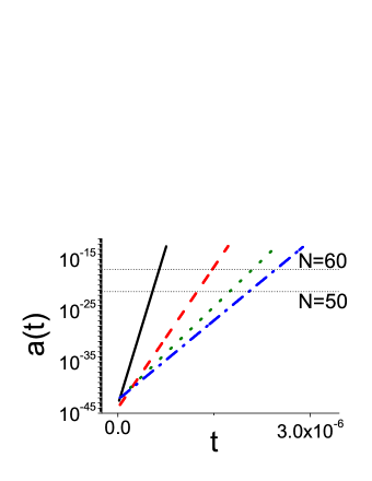
Figure 1: Four inflationary solutions for the Starobinsky ansatz (55), corresponding to a) $m_{g}=10^{-50}$, $\alpha_{3}=2$, $\alpha_{4}=-1$, $a_{k}=5\times 10^{-41}$, $\xi=10^{10}$ (black-solid), b) $m_{g}=10^{-50}$, $\alpha_{3}=10$, $\alpha_{4}=10$, $a_{k}=10^{-41}$, $\xi=10^{9}$ (red-dashed), c) $m_{g}=10^{-50}$, $\alpha_{3}=1$, $\alpha_{4}=1$, $a_{k}=10^{-40}$, $\xi=10^{10}$ (blue-dash-doted), d) $m_{g}=10^{-50}$, $\alpha_{3}=10$, $\alpha_{4}=1$, $a_{k}=2\times 10^{-41}$, $\xi=10^{10}$ (green-dotted). All parameters are in Planck units. The two horizontal lines mark the $N=50$ and $N=60$ e-folding regimes.

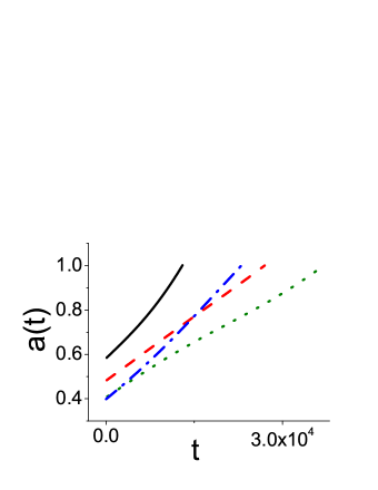
Figure 2: Four late-time accelerating solutions for the Starobinsky ansatz (55), corresponding to a) $m_{g}=2$, $\alpha_{3}=1$, $\alpha_{4}=1$, $a_{k}=0.05$, $\xi=0.2$ (black-solid), b) $m_{g}=1.5$, $\alpha_{3}=1$, $\alpha_{4}=-2$, $a_{k}=0.01$, $\xi=0.5$ (red-dashed), c) $m_{g}=3$, $\alpha_{3}=3$, $\alpha_{4}=-5$, $a_{k}=0.05$, $\xi=0.5$ (blue-dash-doted), d) $m_{g}=3$, $\alpha_{3}=10$, $\alpha_{4}=1$, $a_{k}=0.05$, $\xi=0.5$ (green-doted). All parameters are in units where the present Hubble parameter is $H_{0}=1$, and we have imposed $\Omega_{m0}\approx 0.31$, $\Omega_{DE0}\approx 0.69$, $\Omega_{k0}\approx 0.01$ at the present scale factor $a_{0}=1$ Ade:2013zuv .

Additionally, in Figure 2 we numerically depict four late-time self-accelerating solutions. We would like to mention that in order to handle the late-time evolutions, we need to define the dark energy equation of state $w_{DE}$ and its density parameter $\Omega_{DE}$. In the $F(R)$-literature there are two ways to do it. The first is to use the Friedmann equations in the form of (33), (34), in which we introduce an effective Planck mass square $M_{p}^{2}F_{,R}$, and define $\Omega_{F_{R}}\equiv\rho_{F_{R}}/(3M_{p}^{2}F_{,R}H^{2})$, with $w_{F_{R}}\equiv p_{F_{R}}/\rho_{F_{R}}$ Sotiriou:2008rp . The second method is to rewrite the Friedmann equations in order to have the standard Planck mass square $M_{p}^{2}$ in the left hand side, to absorb the remaining terms in a modified $\bar{\rho}_{F_{R}}$ and $\bar{p}_{F_{R}}$, and to define $\Omega_{F_{R}}\equiv\bar{\rho}_{F_{R}}/(3M_{p}^{2}H^{2})$, with $w_{F_{R}}\equiv\bar{p}_{F_{R}}/\bar{\rho}_{F_{R}}$ DeFelice:2010aj . Despite the fact that in usual cases the difference is small at the background level (and the specific choice has to be made in accordance with the specific measurement method of $M_{p}$, $\Omega_{DE}$ and $w_{DE}$), we stress that the usual conservation equation $\dot{\rho}+3H(\rho+p)=0$ holds only for $\bar{\rho}_{F_{R}}$ and not for $\rho_{F_{R}}$ DeFelice:2010aj . Although, this is not crucial (since we are dealing with modified gravity the dark energy sector is effective, arising from the extra gravitational features, and there is no fundamental reason that it should be conserved), in the present work we follow the second way in order for our model to present energy conservation of the “$F(R)$” sector, and subsequently for the whole dark-energy one. Thus, the matter, curvature and massive-gravity density parameters are defined using $3M_{p}^{2}H^{2}$ too, and they are also conserved.

As we observe from these figures, in this particular choice of the Starobinsky ansatz, the Ricci scalar is relative large at early times, and thus the $R^{2}$ correction term drives a successful inflation. On the other hand, $R$ becomes very small at late times and thus the “$F(R)$” contribution is dramatically suppressed, and therefore the acceleration is driven solely by the effective cosmological constant induced by the graviton mass. Therefore, this model provides a unified description of both inflation and late-time acceleration of the universe. In particular, the corresponding cosmological evolution at the background level provides a specific realization of the Starobinsky-$\Lambda$CDM cosmology. Note however that at the perturbation level the present model will behave differently comparing to Starobinsky-$\Lambda$CDM cosmology, since the graviton sector contributes as well, contrary to the simple cosmological constant which does not. Therefore, strictly speaking, it is a Starobinsky-$\Lambda$CDM-like scenario.

IV.2 Late-time Cosmology

As we mentioned above, in the case where the universe evolves at late times, both the “$F(R)$” and “massive gravity” sectors may contribute effectively to the dark energy component. In particular, the “$F(R)$” contribution brings dynamical features into dark energy physics, and thus it can be of great phenomenological interest. Thus, in this subsection, we focus on the details of late-time evolutions, going beyond the simple effective cosmological constant of the previous subsection, and using viable $F(R)$ forms, which quantitatively describe the observational data.

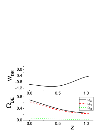
Figure 3: Upper graph: The dark energy equation-of-state parameter $w_{DE}$ as a function of the redshift $z$, in the case of the exponential $F(R)$ ansatz (56), for $m_{g}=1$, $\alpha_{3}=3$, $\alpha_{4}=-2$, $a_{k}=0.1$, $\beta=1.5$, $R_{S}=0.25$. All parameters are in units where the present Hubble parameter is $H_{0}=1$, and we have imposed $\Omega_{m0}\approx 0.31$, $\Omega_{DE0}\approx 0.69$ and $\Omega_{k0}\approx 0.01$ at present Ade:2013zuv . Lower graph: The corresponding evolution of the dark energy density parameter $\Omega_{DE}$ (back-solid), as well as it two constituents $\Omega_{F_{R}}$ (red-dashed) and $\Omega_{MG}$ (green-dotted), of the $F(R)$ and massive-gravity sectors respectively.

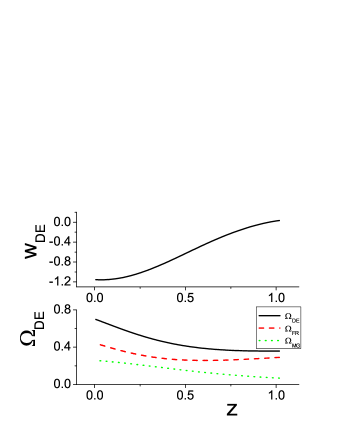
Figure 4: Upper graph: The dark energy equation-of-state parameter $w_{DE}$ as a function of the redshift $z$, in the case of the exponential $F(R)$ ansatz (56), for $m_{g}=0.75$, $\alpha_{3}=1$, $\alpha_{4}=-2$, $a_{k}=0.1$, $\beta=1.1$, $R_{S}=0.3$. All parameters are in units where the present Hubble parameter is $H_{0}=1$, and we have imposed $\Omega_{m0}\approx 0.31$, $\Omega_{DE0}\approx 0.69$ and $\Omega_{k0}\approx 0.01$ at present Ade:2013zuv . Lower graph: The corresponding evolution of the dark energy density parameter $\Omega_{DE}$ (back-solid), as well as its two constituents $\Omega_{F_{R}}$ (red-dashed) and $\Omega_{MG}$ (green-dotted), of the $F(R)$ and massive-gravity sectors respectively.

We would like to examine the two well-known viable $F(R)$ models that are in best agreement with observations. First we consider the $F(R)$ gravity of the exponential ansatz Zhang:2005vt ; Li:2006vi ; Elizalde:2010ts

$$F(R)=R-\beta R_{S}\left(1-e^{-R/R_{S}}\right)~{},$$ (56)

with $R_{S}$ and $\beta$ the model parameters. This ansatz is viable for $\beta>1$ and $R_{S}>0$ Zhang:2005vt , and it is able to fit observations with only one more parameter comparing to the $\Lambda$CDM cosmology. We numerically solve the cosmological system governed by the $F(R)$ massive gravity with this exponential form and we present two different results in Figures 3 and 4, under two different groups of parameter choices, respectively. Our results focus on the dynamics of the equation-of-state parameter of dark energy $w_{DE}$ and the corresponding density parameter $\Omega_{DE}$. For clarity, we also depict the evolutions of both dark energy constituents, namely the separate $F(R)$ density parameter $\Omega_{F_{R}}$ and the massive gravity one $\Omega_{MG}$, where $\Omega_{DE}=\Omega_{F_{R}}+\Omega_{MG}$. For convenience, we use the redshift $z=\frac{a_{0}}{a}-1$ as the variable of the horizontal axis, with the present scale factor $a_{0}$ set to $1$.

In the case of Figure 3 the dark energy is mainly induced by the “$F(R)$” sector, since the “massive gravity” contribution is quite small. On the other hand, in the case of Figure 4, both the “$F(R)$” and “massive gravity” sectors have a significant contribution to $\Omega_{DE}$. One notices that in these specific examples, the equation of state parameter $w_{DE}$ evolves from $w>-1$ into the $w<-1$ regime and hence provides a realization of the quintom scenario. This is known as a capability and advantage of the $F(R)$ gravity models Nojiri:2006ri .

Concerning the phantom-divide crossing realization (see Cai:2009zp for a comprehensive review), there is a well-known “No-Go” theorem which states that any dynamical dark energy with only one single degree of freedom (DoF) in the frame of General Relativity cannot exhibit it, due to severe gradient instabilities in the dispersion relation at the classical level Xia:2007km . In general, in order to circumvent this problems, the quintom models usually involve two scalar DoFs Feng:2004ad , or they are formulated in alternative frameworks such is the non-perturbative string-inspired construction Cai:2007gs , or using a spinor field Cai:2008gk . Interestingly, in the present case of $F(R)$ nonlinear massive gravity, although at linear level we have only one scalar DoF as we will show in section V, its interaction with the graviton potential modifies the dispersion relation which becomes well-behaved when the phantom-divide crossing occurs. Thus, the aforementioned “No-Go” theorem is avoided (this mechanism is similar to the “No-Go” theorem avoidance in the Horndeski models Horndeski:1974wa ; Deffayet:2011gz ).

The second viable and well-studied $F(R)$ ansatz is of the power-law-like Starobinsky form Starobinsky:2007hu ; Capozziello:2007eu :

$$F(R)=R-\lambda R_{c}\bigg{[}1-\left(1+\frac{R^{2}}{R_{c}^{2}}\right)^{-n}\bigg{]}~{},$$ (57)

with $\lambda$, $n$, and $R_{c}$ the (positive) model parameters ($n>0.9$ according to Solar-System constraints Capozziello:2007eu ). We numerically solve the cosmological equations under the above $F(R)$ form and we provide two representative results in Figures 5 and 6, respectively.

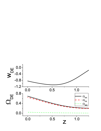
Figure 5: Upper graph: The dark energy equation-of-state parameter $w_{DE}$ as a function of the redshift $z$, in the case of the power-law-like Starobinsky $F(R)$ ansatz (57), for $m_{g}=0.5$, $\alpha_{3}=2$, $\alpha_{4}=1$, $a_{k}=0.1$, $\lambda=0.3$, $n=2$, $R_{c}=2$. All parameters are in units where the present Hubble parameter is $H_{0}=1$, and we have imposed $\Omega_{m0}\approx 0.31$, $\Omega_{DE0}\approx 0.69$ and $\Omega_{k0}\approx 0.01$ at present Ade:2013zuv . Lower graph: The corresponding evolution of the dark energy density parameter $\Omega_{DE}$ (back-solid), as well as its two constituents $\Omega_{F_{R}}$ (red-dashed) and $\Omega_{MG}$ (green-dotted), of the $F(R)$ and massive-gravity sectors respectively.

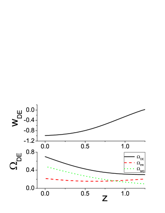
Figure 6: Upper graph: The dark energy equation-of-state parameter $w_{DE}$ as a function of the redshift $z$, in the case of the power-law-like Starobinsky $F(R)$ ansatz (57), for $m_{g}=2$, $\alpha_{3}=2$, $\alpha_{4}=1$, $a_{k}=0.1$, $\lambda=25$, $n=2$, $R_{c}=10$. All parameters are in units where the present Hubble parameter is $H_{0}=1$, and we have imposed $\Omega_{m0}\approx 0.31$, $\Omega_{DE0}\approx 0.69$ and $\Omega_{k0}\approx 0.01$ at present Ade:2013zuv . Lower graph: The corresponding evolution of the dark energy density parameter $\Omega_{DE}$ (back-solid), as well as its two constituents $\Omega_{F_{R}}$ (red-dashed) and $\Omega_{MG}$ (green-dotted), of the $F(R)$ and massive gravity sectors, respectively.

In the case shown in Figure 5, the dynamics of the dark energy is dominated by the contribution of the “$F(R)$” sector, since the “massive gravity” contribution is very small. From the evolution of $w_{DE}$ in this figure, one can see that the quintom scenario occurs twice, thus the universe remains in the phantom regime for a short time. This interesting phenomenological property can be applied in the study of very early universe and a nonsingular bouncing solution can be obtained, similarly to Cai:2007qw . On the other hand, in the case shown in Figure 6, the “massive gravity” sector has the largest contribution at late times, comparing to the $F(R)$ part. Note that the domination of the “massive gravity” sector in Figure 6 makes $w_{DE}$ to approach $-1$ but does not allow for a crossing. This is expected since, as we mentioned after (37), the pure “massive gravity” sector behaves like a cosmological constant (in the case of asymptotic domination of $\Omega_{MG}$ on $\Omega_{F_{R}}$, the $w_{DE}$ tends asymptotically to $-1$).

V Cosmological Perturbations

The scenario of $F(R)$ nonlinear massive gravity is free of the BD ghost, as it is shown in detail in the Appendix. However, it is necessary to examine whether this model remain free of instabilities at the perturbative level. The stability issue of various nonlinear massive gravity models has recently been extensively studied in the literature Gumrukcuoglu:2011zh ; DeFelice:2012mx ; Gumrukcuoglu:2013nza ; Khosravi:2012rk , and the parameter spaces of these models are tightly constrained.

In this section, we proceed to a detailed study of the cosmological perturbations of the scenario at hand, focusing our interest at the level of linear perturbations, and this analysis serves as a completeness of our accompanied work Cai:2013lqa . We work in the unitary gauge which leaves the Stückelberg fields unperturbed. Additionally, as usual we perform the calculations in the Einstein frame, but we drop the tildes on the metric for convenience (thus in this section the dots denote derivatives with respect to the time-variable of the Einstein-frame metric).

The metric variables found in the action, and introduced in Eq. (III.2.2), are perturbed according to the following convention

$$g_{00}=-N^{2}(1+2\phi)~{},$$

$$g_{0i}=Na\beta_{i}~{},$$

$$g_{ij}=a^{2}(\gamma^{K}_{ij}+h_{ij}).$$ (58)

The scalar field is also perturbed as $\varphi\rightarrow\varphi+\delta\varphi$ while the Stückelberg fields are not as we work in the unitary gauge. Therefore, note that in this section the symbol $\varphi$ is used for the scalar field in the Einstein frame, while $\phi$ is used for the scalar metric perturbation (thus no confusion is possible since the Stückelberg fields do not appear).

Then we can further decompose them in a traceless and transverse tensor ($\gamma_{ij}$), transverse vectors ($B_{i},~{}F_{i}$) and scalars ($\phi,~{}B,~{}\psi,~{}E$) parts through the following relations,

$$\beta_{i}=\partial_{i}B+B_{i}~{},~{}~{}D_{i}B^{i}=0,$$ (59)

$$h_{ij}=2\gamma^{K}_{ij}\psi+D_{i}D_{j}E+\frac{1}{2}(D_{i}F_{j}+D_{j}F_{i})+\gamma_{ij},$$ (60)

$$D_{i}F^{i}=D^{i}\gamma_{ij}=0~{},~{}~{}\gamma^{i}_{i}=0~{},$$ (61)

where we have introduced the spatial covariant derivative $D_{i}$ compatible with the background 3-metric $\gamma^{K}_{ij}$.

One can derive the equations of motion of cosmological perturbation by perturbing the extended Einstein’s equation of nonlinear massive gravity. We do not include the contribution from extra matter as it does not change the conclusion. Einstein’s equation can be expressed as

$$\delta G_{\mu\nu}+\delta X_{\mu\nu}=M_{p}^{-2}\delta T_{\mu\nu}~{},$$ (62)

where $G_{\mu\nu}$ is the regular Einstein tensor and the extra term $X_{\mu\nu}$ comes from the “massive gravity” part of the action. For convenience we introduce

$$M_{GW}=\frac{m_{g}^{2}\tilde{\cal B}}{8}(1-\tilde{\cal B})\left[1+(2-\tilde{\cal B})\alpha_{3}+(1-\tilde{\cal B})\alpha_{4}\right]$$

$$\ \ \ \ \ \ \ \ \ \ \ \ +\frac{m_{g}^{2}\tilde{\cal B}}{8}\tilde{Y}_{1}~{},$$ (63)

which will be used in the following calculation.

The process of deriving the perturbed Einstein equations is straightforward. Here we list the non-vanishing equations of motion as follows,

$$3H(H\phi-\dot{\psi})+\frac{D^{2}}{a^{2}}\left[\psi+aH\left(B-\frac{a\dot{E}}{2}\right)\right]+\frac{3a_{k}^{2}\psi}{a^{2}}=$$

$$-\frac{\dot{\varphi}\dot{\delta\varphi}+U_{,\varphi}\delta\varphi}{2}+\frac{\dot{\varphi}^{2}\phi}{2}+\frac{2m_{g}^{2}M_{p}^{2}\Omega_{,\varphi}}{\Omega^{5}}(\tilde{\cal B}-1)\tilde{Y}_{2}\delta\varphi~{},$$ (64)

$$\left[H\phi-\dot{\psi}-\frac{a_{k}}{a}\left(B-\frac{a\dot{E}}{2}\right)\right]_{,i}=\left[\frac{\dot{\varphi}\delta\varphi}{2}\right]_{,i}~{},$$ (65)

$$\ -(3H^{2}+\dot{H})\phi-H\dot{\phi}+\ddot{\psi}+3H\dot{\psi}-\frac{a_{k}^{2}}{a^{2}}(\phi+\psi)$$

$$\ -\frac{D^{2}}{3}\left[\frac{\psi+\phi}{a^{2}}+\frac{2H}{a}\left(B-\frac{a\dot{E}}{2}\right)+\frac{1}{a}\frac{d}{dt}\left(B-\frac{a\dot{E}}{2}\right)\right]$$

$$\ +M_{GW}\psi$$

$$\ =-\frac{\dot{\varphi}\dot{\delta\varphi}-U_{,\varphi}\delta\varphi}{2}-\frac{2m_{g}^{2}M_{p}^{2}\Omega_{,\varphi}}{\Omega^{5}}(\tilde{\cal B}-1)\tilde{Y}_{2}\delta\varphi~{},$$ (66)

$$\left(\frac{D^{2}+3a_{k}^{2}}{a^{2}}\right)\left[\frac{2H}{a}\left(B-\frac{a\dot{E}}{2}\right)+\frac{1}{a}\frac{d}{dt}\left(B-\frac{a\dot{E}}{2}\right)\right.$$

$$\left.\ \ \ \ \ \ \ \ \ \ \ \ \ \ \ \ \ \ \ +\phi+\psi-\frac{M_{GW}}{2}E\right]=0~{},$$ (67)

which correspond to the $(00)$, $(0i)$, $(ii)$, $(ij)$ components, respectively. Additionally, we have the perturbed Klein-Gordon equation for the field fluctuation, which takes the form of

$$\ddot{\delta\varphi}+3H\dot{\delta\varphi}-\frac{D^{2}}{a^{2}}\delta\varphi+U_{,\varphi\varphi}\delta\varphi+2U_{,\varphi}\psi-4\dot{\varphi}\dot{\psi}=$$

$$\ M_{GW}\left(\frac{\dot{\varphi}}{2}\dot{E}-U_{,\varphi}E\right)+8m_{g}^{2}\Omega^{-4}(\tilde{\cal B}-1)\tilde{Y}_{2}\delta\varphi~{},$$ (68)

where the coefficient $\tilde{\cal B}$ is given by (III.2.2).

Since neither $\phi$ nor $\dot{\psi}$ appear as coefficient of the graviton mass term, the kinetic structure is very similar to that of GR. This is seen in many other massive gravity constructions, when one considers the self-accelerating cosmological solution as the background. With this in mind, we are allowed to use the Bardeen potentials,

$$\psi_{B}=-\psi-aH\big{(}B-\frac{a\dot{E}}{2}\big{)}~{},$$

$$\phi_{B}=\phi+\frac{d}{dt}\bigg{[}a\big{(}B-\frac{a\dot{E}}{2}\big{)}\bigg{]}~{},$$

$$\delta\varphi_{B}=\delta\varphi+\dot{\varphi}a\big{(}B-\frac{a\dot{E}}{2}\big{)}~{},$$ (69)

to rewrite the equations and reduce the apparent propagating DoFs in the present model. Making use of the above varialbe, Eq. (V) yields

$$\phi_{B}-\psi_{B}=M_{GW}\frac{E}{2}~{}.$$ (70)

Similar to usual perturbation analysis, it is convenient to define the well-known Mukhanov-Sasaki variable:

$${\cal{Q}}=\delta\varphi_{B}+\frac{\dot{\varphi}}{H}\psi_{B}~{}.$$ (71)

We first combine the $(00)$ and $(ii)$ components of the perturbed Einstein equations, by calculating Eq. (V) minus (V), and then insert the result into the perturbed Klein-Gordon equation (V). In terms of the variable ${\cal{Q}}$, we obtain the perturbation equation as follows:

$$\ddot{\mathcal{Q}}+3H\dot{\cal{Q}}+\left[\frac{D^{2}}{a^{2}}+U_{,\varphi\varphi}-\frac{1}{M_{p}^{2}a^{3}}\frac{d}{dt}\left(\frac{a^{3}}{H}\dot{\varphi}^{2}\right)\right]{\cal{Q}}=$$

$$\frac{2m_{g}^{2}\tilde{Y}_{Q}}{3\Omega^{4}}{\cal{Q}}-\frac{2a_{k}^{2}}{a^{2}H^{2}}\Big{(}\ddot{\varphi}-\frac{\dot{H}\dot{\varphi}}{H}\Big{)}\psi_{B}~{},$$ (72)

where $\tilde{Y}_{Q}\equiv 4(1-\tilde{\cal B})\tilde{Y}_{2}$.

Observing Eq. (V), one deduces that in the scenario at hand the field variable ${\cal{Q}}$ is one propagating DoF characterizing the dynamics of cosmological perturbations. The crucial issue is to examine whether $\psi_{B}$ is a dynamical DoF too, or whether it can be integrated out through some constraint equation.

We first re-express equations (V) and (65) in terms of the Bardeen potentials (V) and ${\cal{Q}}$. Therefore, we can derive the following two useful formulae:

$$\psi_{B} =C^{-1}\left(\frac{\ddot{\varphi}}{2M_{p}^{2}}{\cal{Q}}+\frac{\dot{\varphi}^{3}}{4M_{p}^{4}H}{\cal{Q}}-\frac{\dot{\varphi}}{2M_{p}^{2}}{\dot{\cal{Q}}}\right)~{},$$ (73)

$$\dot{\psi}_{B} =C^{-1}\left(-\frac{\ddot{\varphi}\dot{\varphi}^{2}}{4M_{p}^{4}H}-\frac{\ddot{\varphi}H}{2M_{p}^{2}}+\frac{\dot{H}\dot{\varphi}^{3}}{4M_{p}^{4}H^{2}}\right.$$

$$\left.\ \ \ \ \ \ \ \ \ \ \ \ -\frac{\dot{\varphi}^{3}}{M_{p}^{4}}-\frac{3\dot{H}\dot{\varphi}}{2M_{p}^{2}}-\frac{D^{2}}{a^{2}}\frac{\dot{\varphi}}{2M_{p}^{2}}\right){\cal{Q}}$$

$$\ \ \ +C^{-1}\left(\frac{\dot{\varphi}^{3}}{4M_{p}^{4}H}+\frac{\dot{\varphi}H}{2M_{p}^{2}}\right){\dot{\cal{Q}}}$$

$$\ \ \ +C^{-1}\left(\frac{D^{2}}{a^{2}}+3H\dot{H}+\frac{3H\dot{\varphi}^{2}}{2M_{p}^{2}}\right.$$

$$\left.\ \ \ \ \ \ \ \ \ \ \ \ \ \ \ -\frac{\dot{H}\dot{\varphi}^{2}}{2M_{p}^{2}H}-\frac{\dot{\varphi}^{4}}{2M_{p}^{2}H}\right)M_{GW}\frac{E}{2}~{},$$ (74)

with the operator $C$ defined as

$$C=-\frac{D^{2}}{a^{2}}-3\dot{H}-\frac{3\dot{\varphi}}{2M_{p}^{2}}+\frac{\dot{H}\dot{\varphi}^{2}}{2M_{p}^{2}H^{2}}+\frac{\dot{\varphi}^{4}}{4M_{p}^{4}H^{2}}~{}.$$ (75)

Equations (73) and (74) determine the dynamics of $\psi_{B}$. However, they are not independent since $\frac{d}{dt}\psi_{B}=\dot{\psi}_{B}$. The consistency of their combination, together with the main perturbation equation (V), leads to a strong constraint, namely $E=0$. Hence, we can clearly see that there exists only a single scalar propagating DoF, that is ${\cal{Q}}$, at the linear order in the perturbation theory around the cosmological background.

Let us now examine the stability of the single DoF ${\cal{Q}}$. Inserting (73) into (V), we observe that the sign in front of $\ddot{\cal{Q}}$ remains equal to one, and thus no apparent ghost instability appears. The existence of the term containing $\psi_{B}$ would modify the dispersion relation of the gradient terms. But in a realistic cosmological background the spatial curvature term is observationally suppressed and thus the corresponding effect on modifying the dispersion relation would be secondary. The last interesting property shown in Equation (V) is the term proportional to $m_{g}^{2}$. Obviously, this is a new term brought by the gravitational potential and thus it is interpreted as the effective mass of the scalar graviton. Despite the corrections from other terms, one deduces that if $\tilde{Y}_{Q}<0$ then the model is free of tachyonic instabilities. Note that this requirement still leaves a large part of the parameter space, and thus a huge class of interesting cosmological behavior.

We close this section by making some comments on the comparison with other extended nonlinear massive gravity models, such are the quasi-dilaton massive gravity D'Amico:2012zv and the mass-varying massive gravity Huang:2012pe , following the discussion of section II. From the point of view of perturbation analysis, both the quasi-dilaton and mass-varying massive gravity models involve at least two scalar DoF, one introduced by the additional scalar field and the other being the longitudinal mode of the graviton. This can be verified by counting the number of nonzero eigenvalues of the matrix for the kinetic part of the perturbation action Gumrukcuoglu:2013nza . Applying the method of Gumrukcuoglu:2013nza in the present scenario of $F(R)$ nonlinear massive gravity (this can be performed immediately by taking the results of Gumrukcuoglu:2013nza and set the coefficient in front of the scalar-field kinetic term to unity), we find that there exists only one nonzero eigenvalue in our model, and this implies only a single DoF. Thus, the present model is radically different from the aforementioned two.

VI Conclusions

Recently, a nonlinear massive gravity theory was constructed in deRham:2010ik , in which the BD ghost can be removed in the decoupling limit to all orders in perturbation theory, through a systematic construction of a covariant nonlinear action. The theoretical advantages of such a construction led to a wide investigation of its cosmological implications deRham:2010tw ; Gumrukcuoglu:2011ew , as well as of the black hole solutions Koyama:2011xz , while the connections to bi-metric and multi-metric gravity were also revealed Damour:2002wu ; Hassan:2011tf . However, the cosmological perturbations around these solutions are found to exhibit in general severe instabilities DeFelice:2012mx , and thus extensions of the basic theory are necessary.

In this work, we constructed the $F(R)$ extension of nonlinear massive gravity, as an accompanied paper to our previous work Cai:2013lqa , focusing on a detailed cosmological investigation, both at the background and perturbation levels. In particular, we investigated three representative cosmological evolutions. In the first one we considered the $F(R)$ sector to be of the Starobinsky’s $R^{2}$-form and we explicitly showed that this model can describe both inflation and late time acceleration in a unified picture, with the $F(R)$ sector driving inflation and the graviton mass responsible for dark energy. Furthermore, we studied the case in which $F(R)$ takes the usual viable exponential form and we showed that this class of models can easily quantitatively describe the late-time universe behavior, including the possibility of a phantom-divide crossing. In the last example we considered the power-law-like Starobinsky $F(R)$ ansantz, which is another viable form, with similar quantitative behavior. In these two classes of evolutions, the effective dark energy component includes contributions from both sectors, namely the $F(R)$ and the massive graviton one.

Apart from the interesting cosmological implications at the background level, the advantage of the present scenario is the behavior of cosmological perturbations. We developed the perturbations by expanding the Einstein equations to linear order, around a cosmological solution. Although the dispersion relation of the scalar mode is different from the case of GR, the effect is negligible in a realistic cosmological background due to the suppression of the curvature term. Our analysis showed that there exists only one propagating scalar mode in this model, which can additionally be free of ghost instabilities in a large part of the parameter space. This issue is the crucial difference of $F(R)$ nonlinear massive gravity comparing to other extensions, such are the quasi-dilaton and the varying-mass massive gravity. The fact that both $F(R)$ and massive graviton sectors are needed for this behavior, may imply that the UV and IR modifications of gravity may not be independent.

At the end of the present work, we would like to highlight one interesting property of the specific model of $R^{2}$-massive gravity. One notices that, the effective potential for the scalar field after conformal transformation, approaches a constant in the UV regime. This extremely flat potential, which can be applied to drive sufficiently long inflationary process at early universe as analyzed in Sec. IV.1, indicates an approximately shift symmetry along the scalar field. This feature interestingly coincides with the model of quasi-dilaton massive gravity with a specifically chosen dilatonic parameter. However, when the scalar field evolves into the IR regime, it is stabilized at the vacuum and hence this shift symmetry can be spontaneously broken. This profound property is interesting to the process of symmetry breaking in nonlinear massive gravity models, and deserves further investigations.

Appendix A Hamiltonian Constraint Analysis

In this appendix we perform a Hamiltonian constraint analysis of $F(R)$ nonlinear massive gravity, and we show that the potentially dangerous extra mode of graviton scalar vanishes due to the existence of a secondary constraint. We follow the method developed in Hassan:2011hr (see also Cai:2013lqa ; Kluson:2013yaa ), and we reproduce the major derivation for completeness. As usual, we perform the analysis in the Einstein frame based on the Lagrangian (13), and we drop the tilde-subscripts for convenience.

Using the ADM formalism one can decompose the physical and fiducial metric as

$$\tilde{g}_{\mu\nu}dx^{\mu}dx^{\nu}=-(N_{g}^{0})^{2}dt^{2}+\gamma_{ij}(dx^{i}+N_{g}^{i}dt)(dx^{j}+N_{g}^{j}dt),$$

$$f_{\sigma\rho}dx^{\sigma}dx^{\rho}=-(N_{f}^{0})^{2}dt^{2}+\omega_{ab}(dx^{a}+N_{f}^{a}dt)(dx^{b}+N_{f}^{b}dt).$$ (76)

Amongst all the coefficients in the metrics, the lapse $N_{g}^{0}$ and the shift $\vec{N}_{g}$ (the three $N_{g}^{i}$’s expressed as vector) of the physical metric, as well as the corresponding ones for the fiducial metric, $N_{f}^{0}$ and $\vec{N}_{f}$ respectively, are not dynamical DoFs.

In general massive gravity $\gamma_{ij}$ allows for at most six propagating modes, one of them being the origin of the BD ghost. Thus, a potentially healthy theory must maintain a single constraint on ${\bar{\gamma}}$ (from now on a bar denotes the matrix form) and the corresponding conjugate momenta, along with an associated secondary constraint, which will lead to the elimination of the ghost DoF. In the following we show the existence of these constraints in $F(R)$ massive gravity.

In general, the propagating DoFs are the $\{\gamma_{ij},\varphi\}$, such that their phase space spans $14$ dimensions after including their conjugate momentas $\{\pi_{ij},\pi\}$. In standard GR, four ghostly propagating DoF are eliminated by the constraints from the equations of motion of the lapse $N$ and shifts $N^{i}$. The inclusion of a generic mass term changes these equations and they do not directly give rise to any constraints on $\gamma_{ij}$. However, the dRGT mass term is such that the four equations of motion for $N$ and $N^{i}$ give rise to an equation independent of $N$ and $N^{i}$, which provides a constraint that eliminates one potentially dangerous DoF. Consistency of the first constraint to be valid at later times introduces a secondary constraint. These are necessary since we expect massive gravity to have only five propagating DoF carried by $\gamma_{ij}$. The extra $6$-th mode carried by the helicity $0$ mode is at the origin of the BD ghost.

We can make this constraint explicit by introducing a Lagrange multiplier in the action. This is done by using a new shift function $n^{i}$ defined through the following relation:

$$N^{i}-L^{i}=(L\delta^{i}_{j}+ND^{i}_{j})n^{j},$$ (77)

where $D^{i}_{j}$ is determined by

$$\sqrt{(1-n^{i}\xi_{ij}n^{j})}D^{i}_{j}=\sqrt{(\gamma^{ik}-D^{i}_{m}n^{m}D^{k}_{l}n^{l})\xi_{kj}}.$$

The explicit form of $D$ is not needed for the analysis, but without loss of generality we apply the expression that satisfies the identity $\xi D=D\xi$. Defining $\lambda=(1-n^{i}\xi_{ij}n^{j})$, the Hamiltonian can be written as

$$H=\int d^{3}x\mathcal{H}=\int d^{3}x(\mathcal{H}_{0}+N\mathcal{C})~{},$$ (78)

with

$$\mathcal{H}_{0} =-(Ln^{i}+L^{i})\mathcal{R}_{i}-L\sqrt{\gamma}\mathcal{A}m_{g}^{2}M_{p}^{2}$$

$$\mathcal{C} =\mathcal{R}+\mathcal{R}_{i}D^{i}_{j}n^{j}+\sqrt{\gamma}\mathcal{B}m_{g}^{2}M_{p}^{2}~{},$$

where

$$\mathcal{R}=\frac{\sqrt{\gamma}}{2}\left[M_{p}^{2}\text{}^{(3)}R-\partial_{i}\varphi\partial^{i}\varphi-2U(\varphi)\right.$$

$$\left.\ \ \ \ \ \ +\frac{1}{\gamma}\left(\frac{1}{M_{p}^{2}}\pi^{i}_{i}\pi^{j}_{j}-\frac{2}{M_{p}^{2}}\pi^{ij}\pi_{ij}-\frac{1}{2}\pi^{2}\right)\right]~{},$$

$$\mathcal{R}_{i}=2\gamma_{ij}\nabla_{k}\pi^{jk}-\pi\partial_{i}\varphi~{},$$

$$\mathcal{A}=\tilde{\beta}_{1}\lambda^{1/2}+\tilde{\beta}_{2}\left[\lambda D^{i}_{i}+n^{i}\xi_{ij}D^{j}_{k}n^{k}\right]+\tilde{\beta}_{4}\sqrt{\frac{\xi}{\gamma}}$$

$$\ \ \ \ \ \ +\tilde{\beta}_{3}\left[2\lambda^{1/2}D^{[l}_{l}n^{i]}\xi_{ij}D^{i}_{k}n^{k}+\lambda^{3/2}D^{[i}_{i}D^{j]}_{j}\right],$$

$$\mathcal{B}=\tilde{\beta}_{0}+\tilde{\beta}_{1}\lambda^{1/2}D^{i}_{j}+\tilde{\beta}_{2}\lambda D^{[i}_{i}D^{j]}_{j}+\tilde{\beta}_{3}\lambda^{3/2}D^{[i}_{i}D^{j}_{j}D^{k]}_{k}~{}.$$ (79)

One can observe that the Hamiltonian (78) is not linear in $n^{i}$ and hence the equations of motion $\frac{\delta\mathcal{L}}{\delta n^{i}}=\mathcal{C}_{i}=0$ do not lead to any constraints on the propagating DoFs, but they determine $n^{i}(\gamma_{ij},\pi^{ij},\varphi,\pi)$. However, (78) is now linear in $N$, and thus $\frac{\delta\mathcal{L}}{N}=\mathcal{C}=0$ provides our first constraint on the system.

Consistency requires that $\mathcal{C}=0$ is valid at all times. If this is trivially satisfied, then there would be no additional constraints. Fortunately, we find that the derivative

$$\frac{d}{dt}\mathcal{C}(x)=\{\mathcal{C}(x),H\}\ \ \ \ \ \ \ \ \ \ \ \ \ \ \ \ \ \ \ \ \ \ \ \ \ \ \,\ \ \ \ \ \ \ \ \ \ \ \ \ \ \ \$$

$$=\int d^{3}y\left[\{\mathcal{C}(x),H_{0}(y)\}-N(y)\{\mathcal{C}(x),\mathcal{C}(y)\}\right]$$ (80)

does not vanish trivially, and this indicates that it does imposes the secondary constraint needed to eliminate the ghost. In the above we have introduced the Poisson brackets

$$\{\mathcal{O}_{1}(x),\mathcal{O}_{2}(y)\} =\int d^{3}z\left[\frac{\delta\mathcal{O}_{1}(x)}{\delta\gamma_{mn}(z)}\frac{\delta\mathcal{O}_{2}(y)}{\delta\pi^{mn}(z)}\right.$$

$$\left.\ \ \ \ \ \ \ \ \ \ \ \ \ \ -\frac{\delta\mathcal{O}_{1}(x)}{\delta\pi^{mn}(z)}\frac{\delta\mathcal{O}_{2}(y)}{\delta\gamma_{mn}(z)}\right]$$

$$~{}~{}+\int d^{3}z\left[\frac{\delta\mathcal{O}_{1}(x)}{\delta\varphi(z)}\frac{\delta\mathcal{O}_{2}(y)}{\delta\pi(z)}\right.$$

$$\left.\ \ \ \ \ \ \ \ \ \ \ \ \ \ -\frac{\delta\mathcal{O}_{1}(x)}{\delta\pi(z)}\frac{\delta\mathcal{O}_{2}(y)}{\delta\varphi(z)}\right]~{}.$$ (81)

First of all, we need to prove that $\{\mathcal{C}(x),\mathcal{C}(y)\}=0$. Otherwise, the appearance of the lapse $N$ in (A) would not turn this consistency requirement into a constraint on the propagating modes as: $\mathcal{C}^{(2)}=\int d^{3}y\{\mathcal{C}(x),\mathcal{H}_{0}(y)\}=0$. Straightforwardly we calculate

$$\{\mathcal{C}(x),\mathcal{C}(y)\}=\{\mathcal{R}(x),\mathcal{R}(y)\}$$

$$\ +\{\mathcal{R}_{i}(x),\mathcal{R}_{j}(y)\}D^{i}_{k}n^{k}(x)D^{i}_{l}n^{l}(y)$$

$$\ +\left[\{\mathcal{R}(x),\mathcal{R}_{i}(y)\}D^{i}_{k}n^{k}(y)+S^{mn}(x)\frac{\delta\mathcal{R}_{i}(y)}{\delta\pi^{mn}(x)}D^{i}_{k}n^{k}(y)\right.$$

$$\ \left.-\{\mathcal{R}(y),\mathcal{R}_{i}(x)\}D^{i}_{k}n^{k}(x)+S^{mn}(y)\frac{\delta\mathcal{R}_{i}(x)}{\delta\pi^{mn}(y)}D^{i}_{k}n^{k}(x)\right],$$ (82)

with $S^{mn}(x)=\mathcal{R}_{j}\frac{\partial(D^{j}_{r}n^{r})}{\partial\gamma_{mn}}(x)+m_{g}^{2}M_{p}^{2}\frac{\partial(\sqrt{\gamma}\mathcal{B})}{\partial\gamma_{mn}}(x)$. The involved poisson brackets read

$$\{\mathcal{R}(x),\mathcal{R}(y)\} =-\left[\mathcal{R}^{i}(x)\partial_{x^{i}}\delta^{(3)}(x-y)\right.$$

$$\left.\ \ \ \ \ \ \ \ -\mathcal{R}^{i}(y)\partial_{y^{i}}\delta^{(3)}(x-y)\right],$$

$$\{\mathcal{R}(x),\mathcal{R}_{i}(y)\} =-\mathcal{R}(y)\partial_{x^{i}}\delta^{(3)}(x-y),$$

$$\{\mathcal{R}_{i}(x),\mathcal{R}_{j}(y)\} =-\left[\mathcal{R}_{j}(x)\partial_{x^{i}}\delta^{(3)}(x-y)\right.$$

$$\left.\ \ \ \ \ \ \ \ -\mathcal{R}_{i}(y)\partial_{y^{j}}\delta^{(3)}(x-y)\right].$$ (83)

In order to deal with the delta functions, the smoothing functions $f(x)$ and $g(x)$ are introduced as follows,

$$F=\int d^{3}xf(x)\mathcal{C}(x)~{},~{}~{}G=\int d^{3}yg(y)\mathcal{C}(y)~{},$$ (84)

and their Poisson bracket can be evaluated as

$$\{F,G\}=\int d^{3}xd^{3}yf(x)g(x)\{\mathcal{C}(x),\mathcal{C}(y)\}$$

$$\ \ \ \ \ \ \ \ \ \ =-\int d^{3}x(f\partial_{i}g-g\partial_{i}f)P^{i},$$ (85)

where $P^{i}=(\mathcal{R}+\mathcal{R}_{j}D^{j}_{k}n^{k})D^{i}_{l}n^{l}+\mathcal{R}^{i}+S^{il}\gamma_{il}D^{j}_{k}n^{k}$. Accordingly, we can simplify the Poisson bracket of ${\mathcal{C}}$ as

$$\{\mathcal{C}(x),\mathcal{C}(y)\}=\left[P^{i}(x)\partial_{x^{i}}\delta^{(3)}(x-y)-P^{i}(y)\partial_{y^{i}}\delta^{(3)}(x-y)\right].$$

Since we have $P^{i}=\mathcal{C}D^{i}_{l}n^{l}+\mathcal{C}_{j}\gamma^{ji}\big{|}_{\mathcal{C}=0,~{}\mathcal{C}_{j}=0}=0$, we finally explicitly prove that

$$\{\mathcal{C}(x),\mathcal{C}(y)\}=0~{}.$$ (86)

In summary, our consistency condition is therefore $\mathcal{C}^{(2)}=\int d^{3}y\{\mathcal{C}(x),\mathcal{H}_{0}(y)\}=0$, where the Poisson bracket in the integrand writes as

$$\{\mathcal{C}(x),\mathcal{H}_{0}(y)\} =-\{\mathcal{R}(x),\mathcal{R}_{i}(y)\}(Ln^{i}+L^{i})(y)$$

$$\ \ \ -D^{i}_{k}n^{k}(x)\{\mathcal{R}_{i}(x),\mathcal{R}_{j}(y)\}(Ln^{j}+L^{j})(y)$$

$$\ \ \ -S^{mn}(x)\frac{\delta\mathcal{R}_{i}(y)}{\delta\pi^{mn}(x)}(Ln^{i}+L^{i})$$

$$\ \ \ -\sqrt{\gamma}m_{g}^{2}M_{p}^{2}\frac{\partial\mathcal{B}}{\partial\varphi}\frac{\partial\mathcal{R}_{i}}{\partial\pi}(Ln^{i}+L^{i})\delta^{(3)}(x-y)$$

$$\ \ \ +L\sqrt{\gamma}m_{g}^{2}M_{p}^{2}\left[\frac{\delta\mathcal{R}(x)}{\delta\pi^{mn}(y)}A^{mn}(y)\right.$$

$$\ \ \ \ \ \ \ \ +D^{i}_{k}n^{k}(x)\frac{\delta\mathcal{R}_{i}(y)}{\delta\pi^{mn}(x)}A^{mn}(y)$$

$$\ \ \ \ \ \ \ \ +\frac{\partial\mathcal{A}}{\partial\varphi}\frac{\partial\mathcal{R}}{\partial\pi}\delta^{(3)}(x-y)$$

$$\ \ \ \ \ \ \ \ \left.+\frac{\partial\mathcal{B}}{\partial\varphi}\frac{\partial\mathcal{R}_{i}}{\partial\pi}(D^{i}_{k}n^{k})\delta^{(3)}(x-y)\right],$$

with $A^{mn}=\frac{1}{\sqrt{\gamma}}\frac{\partial(\sqrt{\gamma}\mathcal{A})}{\partial\gamma_{mn}}$. After some algebra we finally obtain

$$\mathcal{C}^{(2)} =\mathcal{C}\nabla_{i}(Ln^{i}+L^{i})+m_{g}^{2}M_{p}^{2}(\gamma_{mn}\pi^{k}_{k}-2\pi_{mn})A^{mn}$$

$$\ \ \ +2L\sqrt{\gamma}m_{g}^{2}M_{p}^{2}(\nabla_{m}A^{mn})\gamma_{ni}D^{i}_{k}n^{k}$$

$$\ \ \ +(\mathcal{R}_{j}D^{i}_{k}n^{k}-m_{g}^{2}M_{p}^{2}\sqrt{\gamma}\gamma_{jk}\bar{\mathcal{B}}^{ki})\nabla_{i}(Ln^{j}+L^{j})$$

$$\ \ \ -m_{g}^{2}M_{p}^{2}\sqrt{\gamma}\frac{\partial\mathcal{B}}{\partial\varphi}\partial_{i}\varphi(Ln^{i}+L^{i})$$

$$\ \ \ -m_{g}^{2}M_{p}^{2}L\frac{\partial\mathcal{A}}{\partial\varphi}\partial_{i}\varphi D^{i}_{k}n^{k}~{},$$ (87)

where we have defined

$$\bar{\mathcal{B}}^{mn}= \gamma^{mi}\left\{\tilde{\beta}_{1}\lambda^{-1/2}\xi_{ik}(D^{-1})^{k}_{j}+\tilde{\beta}_{2}\left[\xi_{ik}(D^{-1})^{k}_{j}D^{l}_{l}-\xi_{ij}\right]\right.$$

$$+\tilde{\beta}_{3}\lambda^{1/2}\left[\xi_{ik}D^{k}_{j}-\xi_{ij}D^{k}_{k}\right.$$

$$\left.\left.\ \ \ \ \ \ \ \ \ \ \ \ \ +\frac{1}{2}\xi_{ik}(D^{-1})^{k}_{j}(D^{l}_{l}D^{k}_{k}-D^{l}_{k}D^{k}_{l})\right]\right\}\gamma^{jn}.$$

We mention that $\mathcal{C}$ appears only in the first term of (A), and thus this expression does not automatically vanish on the constraint surface defined by $\mathcal{C}=0$. Therefore, demanding that $\mathcal{C}^{(2)}=0$, imposes the secondary constraint that we needed.

Lastly, a further check needs to be performed, in order to show that no tertiary constraint exists. This is achieved by demonstrating that $\{\mathcal{C}^{(2)}(x),\mathcal{H}_{0}\}\neq 0$ and $\{\mathcal{C}^{(2)}(x),\mathcal{C}(y)\}\neq 0$. Therefore the consistency condition,

$$\frac{d}{dt}\mathcal{C}^{(2)}(x)=\{\mathcal{C}^{(2)}(x),H\}=0~{},$$

gives an equation that determines $N$.

References

- (1) P. A. R. Ade et al. [Planck Collaboration], arXiv:1303.5076 [astro-ph.CO].
- (2) T. P. Sotiriou and V. Faraoni, Rev. Mod. Phys. 82, 451 (2010).
- (3) A. De Felice and S. Tsujikawa, Living Rev. Rel. 13, 3 (2010).
- (4) S. ’i. Nojiri and S. D. Odintsov, Phys. Rept. 505, 59 (2011).
- (5) A. A. Starobinsky, Phys. Lett. B 91, 99 (1980).
- (6) P. A. R. Ade et al. [Planck Collaboration], arXiv:1303.5082 [astro-ph.CO].
- (7) S. M. Carroll, V. Duvvuri, M. Trodden and M. S. Turner, Phys. Rev. D 70, 043528 (2004); S. Capozziello, S. Carloni and A. Troisi, Recent Res. Dev. Astron. Astrophys. 1, 625 (2003); S. M. Carroll, A. De Felice, V. Duvvuri, D. A. Easson, M. Trodden and M. S. Turner, Phys. Rev. D 71, 063513 (2005).
- (8) S. ’i. Nojiri and S. D. Odintsov, Phys. Rev. D 68, 123512 (2003).
- (9) M. Fierz and W. Pauli, Proc. Roy. Soc. Lond. A 173, 211 (1939).
- (10) D. G. Boulware and S. Deser, Phys. Rev. D 6, 3368 (1972).
- (11) C. de Rham and G. Gabadadze, Phys. Rev. D 82, 044020 (2010); C. de Rham, G. Gabadadze and A. J. Tolley, Phys. Rev. Lett. 106, 231101 (2011).
- (12) S. F. Hassan and R. A. Rosen, Phys. Rev. Lett. 108, 041101 (2012) [arXiv:1106.3344 [hep-th]]; S. F. Hassan and R. A. Rosen, JHEP 1204, 123 (2012).
- (13) C. de Rham, G. Gabadadze and A. J. Tolley, Phys. Lett. B 711, 190 (2012); C. de Rham, G. Gabadadze and A. J. Tolley, JHEP 1111, 093 (2011).
- (14) K. Hinterbichler, Rev. Mod. Phys. 84, 671 (2012).
- (15) C. de Rham, G. Gabadadze, L. Heisenberg and D. Pirtskhalava, Phys. Rev. D 83, 103516 (2011); G. D’Amico, C. de Rham, S. Dubovsky, G. Gabadadze, D. Pirtskhalava and A. J. Tolley, Phys. Rev. D 84, 124046 (2011); K. Koyama, G. Niz and G. Tasinato, JHEP 1112, 065 (2011); D. Comelli, M. Crisostomi, F. Nesti and L. Pilo, JHEP 1203, 067 (2012) [Erratum-ibid. 1206, 020 (2012)]; D. Comelli, M. Crisostomi and L. Pilo, JHEP 1206, 085 (2012); V. F. Cardone, N. Radicella and L. Parisi, Phys. Rev. D 85, 124005 (2012); P. Gratia, W. Hu and M. Wyman, Phys. Rev. D 86, 061504 (2012); T. Kobayashi, M. Siino, M. Yamaguchi and D. Yoshida, Phys. Rev. D 86, 061505 (2012); D. Langlois and A. Naruko, Class. Quant. Grav. 29, 202001 (2012); Y. -l. Zhang, R. Saito and M. Sasaki, JCAP 1302, 029 (2013); G. Leon, J. Saavedra and E. N. Saridakis, Class. Quant. Grav. 30, 135001 (2013); K. Hinterbichler, J. Stokes and M. Trodden, Phys. Lett. B 725, , 1 (2013); K. Zhang, P. Wu and H. Yu, Phys. Rev. D 87, 063513 (2013); M. Andrews, G. Goon, K. Hinterbichler, J. Stokes and M. Trodden, Phys. Rev. Lett. 111, 061107 (2013) [arXiv:1303.1177 [hep-th]]; M. S. Volkov, Class. Quant. Grav. 30, 184009 (2013); G. Tasinato, K. Koyama and G. Niz, Class. Quant. Grav. 30, 184002 (2013); H. Li and Y. Zhang, arXiv:1304.4780 [gr-qc]; N. Khosravi, G. Niz, K. Koyama and G. Tasinato, JCAP 1308, 044 (2013); Q. -G. Huang, K. -C. Zhang and S. -Y. Zhou, JCAP 1308, 050 (2013); T. Q. Do and W. F. Kao, Phys. Rev. D 88, 063006 (2013); M. Sasaki, D. -h. Yeom and Y. -l. Zhang, Class. Quant. Grav. 30, 232001 (2013); Y. -l. Zhang, R. Saito, D. -h. Yeom and M. Sasaki, arXiv:1312.0709 [hep-th]; S. I. Vacaru, arXiv:1401.2882 [physics.gen-ph].
- (16) A. E. Gumrukcuoglu, C. Lin and S. Mukohyama, JCAP 1111, 030 (2011); A. E. Gumrukcuoglu, C. Lin and S. Mukohyama, Phys. Lett. B 717, 295 (2012); A. De Felice, A. E. Gumrukcuoglu and S. Mukohyama, Phys. Rev. D 88, 124006 (2013).
- (17) A. De Felice, A. E. Gumrukcuoglu and S. Mukohyama, Phys. Rev. Lett. 109, 171101 (2012); A. De Felice, A. E. Gumrukcuoglu, C. Lin and S. Mukohyama, JCAP 1305, 035 (2013); A. De Felice, A. E. Gumrukcuoglu, C. Lin and S. Mukohyama, Class. Quant. Grav. 30, 184004 (2013).
- (18) Y. -F. Cai, F. Duplessis and E. N. Saridakis, Phys. Rev. D 90, 064051 (2014).
- (19) G. D’Amico, G. Gabadadze, L. Hui and D. Pirtskhalava, Phys. Rev. D 87, 064037 (2013).
- (20) R. Gannouji, M. . W. Hossain, M. Sami and E. N. Saridakis, Phys. Rev. D 87, 123536 (2013); K. Bamba, M. . W. Hossain, S. Nojiri, R. Myrzakulov and M. Sami, arXiv:1309.6413 [hep-th].
- (21) Q. -G. Huang, Y. -S. Piao and S. -Y. Zhou, Phys. Rev. D 86, 124014 (2012).
- (22) E. N. Saridakis, Class. Quant. Grav. 30, 075003 (2013); Y. -F. Cai, C. Gao and E. N. Saridakis, JCAP 1210, 048 (2012); D. -J. Wu, Y. -S. Piao and Y. -F. Cai, Phys. Lett. B 721, 7 (2013).
- (23) S. ’i. Nojiri and S. D. Odintsov, Phys. Lett. B 716, 377 (2012); S. ’i. Nojiri, S. D. Odintsov and N. Shirai, JCAP 1305, 020 (2013); K. Bamba, Y. Kokusho, S. ’i. Nojiri and N. Shirai, arXiv:1310.1460 [hep-th].
- (24) P. Zhang, Phys. Rev. D 73, 123504 (2006); G. Cognola, E. Elizalde, S. Nojiri, S. D. Odintsov, L. Sebastiani and S. Zerbini, Phys. Rev. D 77, 046009 (2008); E. V. Linder, Phys. Rev. D 80, 123528 (2009).
- (25) B. Li and M. -C. Chu, Phys. Rev. D 74, 104010 (2006); Y. -S. Song, W. Hu and I. Sawicki, Phys. Rev. D 75, 044004 (2007); R. Bean, D. Bernat, L. Pogosian, A. Silvestri and M. Trodden, Phys. Rev. D 75, 064020 (2007); P. -J. Zhang, Phys. Rev. D 76, 024007 (2007); P. Zhang, M. Liguori, R. Bean and S. Dodelson, Phys. Rev. Lett. 99, 141302 (2007); K. Bamba, C. -Q. Geng and C. -C. Lee, JCAP 1008, 021 (2010).
- (26) E. Elizalde, S. Nojiri, S. D. Odintsov, L. Sebastiani and S. Zerbini, Phys. Rev. D 83, 086006 (2011).
- (27) S. ’i. Nojiri and S. D. Odintsov, eConf C 0602061, 06 (2006) [Int. J. Geom. Meth. Mod. Phys. 4, 115 (2007)]; S. ’i. Nojiri and E. N. Saridakis, Astrophys. Space Sci. 1, 2013 (347).
- (28) Y. -F. Cai, E. N. Saridakis, M. R. Setare and J. -Q. Xia, Phys. Rept. 493, 1 (2010).
- (29) J. -Q. Xia, Y. -F. Cai, T. -T. Qiu, G. -B. Zhao and X. Zhang, Int. J. Mod. Phys. D 17, 1229 (2008).
- (30) B. Feng, X. -L. Wang and X. M. Zhang, Phys. Lett. B 607, 35 (2005); Y. -F. Cai, H. Li, Y. -S. Piao and X. -M. Zhang, Phys. Lett. B 646, 141 (2007).
- (31) Y. -F. Cai, M. -z. Li, J. -X. Lu, Y. -S. Piao, T. -t. Qiu and X. -m. Zhang, Phys. Lett. B 651, 1 (2007).
- (32) Y. -F. Cai and J. Wang, Class. Quant. Grav. 25, 165014 (2008); Y. -F. Cai, M. Li and X. Zhang, Phys. Lett. B 718, 248 (2012); Y. -F. Cai, Y. Wan and X. Zhang, arXiv:1312.0740 [hep-th].
- (33) G. W. Horndeski, Int. J. Theor. Phys. 10, 363 (1974).
- (34) C. Deffayet, X. Gao, D. A. Steer and G. Zahariade, Phys. Rev. D 84, 064039 (2011).
- (35) A. A. Starobinsky, JETP Lett. 86, 157 (2007); S. Tsujikawa, K. Uddin and R. Tavakol, Phys. Rev. D 77, 043007 (2008); S. K. Chakrabarti, E. N. Saridakis and A. A. Sen, Gen. Rel. Grav. 43, 3065 (2011).
- (36) S. Capozziello and S. Tsujikawa, Phys. Rev. D 77, 107501 (2008).
- (37) Y. -F. Cai, T. Qiu, Y. -S. Piao, M. Li and X. Zhang, JHEP 0710, 071 (2007); Y. -F. Cai, T. Qiu, R. Brandenberger, Y. -S. Piao and X. Zhang, JCAP 0803, 013 (2008); Y. -F. Cai, T. -t. Qiu, J. -Q. Xia and X. Zhang, Phys. Rev. D 79, 021303 (2009); Y. -F. Cai and X. Zhang, JCAP 0906, 003 (2009); Y. -F. Cai, T. -t. Qiu, R. Brandenberger and X. -m. Zhang, Phys. Rev. D 80, 023511 (2009); Y. -F. Cai and X. Zhang, Phys. Rev. D 80, 043520 (2009).
- (38) A. E. Gumrukcuoglu, C. Lin and S. Mukohyama, JCAP 1203, 006 (2012).
- (39) A. E. Gumrukcuoglu, K. Hinterbichler, C. Lin, S. Mukohyama and M. Trodden, Phys. Rev. D 88, 024023 (2013).
- (40) N. Khosravi, H. R. Sepangi and S. Shahidi, Phys. Rev. D 86, 043517 (2012); G. D’Amico, Phys. Rev. D 86, 124019 (2012) [arXiv:1206.3617 [hep-th]]; M. Fasiello and A. J. Tolley, JCAP 1211, 035 (2012); Z. Haghani, H. R. Sepangi and S. Shahidi, Phys. Rev. D 87, 124014 (2013); G. D’Amico, G. Gabadadze, L. Hui and D. Pirtskhalava, Class. Quant. Grav. 30, 184005 (2013) [arXiv:1304.0723 [hep-th]]. M. Andrews, K. Hinterbichler, J. Stokes and M. Trodden, Class. Quant. Grav. 30, 184006 (2013).
- (41) K. Koyama, G. Niz and G. Tasinato, Phys. Rev. Lett. 107, 131101 (2011); T. .M. Nieuwenhuizen, Phys. Rev. D 84, 024038 (2011); K. Koyama, G. Niz and G. Tasinato, Phys. Rev. D 84, 064033 (2011); G. Chkareuli and D. Pirtskhalava, Phys. Lett. B 713, 99 (2012); A. Gruzinov and M. Mirbabayi, Phys. Rev. D 84, 124019 (2011); D. Comelli, M. Crisostomi, F. Nesti and L. Pilo, Phys. Rev. D 85, 024044 (2012); L. Berezhiani, G. Chkareuli, C. de Rham, G. Gabadadze and A. J. Tolley, Phys. Rev. D 85, 044024 (2012); S. Sjors and E. Mortsell, JHEP 1302, 080 (2013); C. -I. Chiang, K. Izumi and P. Chen, JCAP 1212, 025 (2012); Y. -F. Cai, D. A. Easson, C. Gao and E. N. Saridakis, Phys. Rev. D 87, 064001 (2013); E. Babichev and A. Fabbri, Class. Quant. Grav. 30, 152001 (2013); R. Brito, V. Cardoso and P. Pani, Phys. Rev. D 88, 023514 (2013).
- (42) T. Damour, I. I. Kogan and A. Papazoglou, Phys. Rev. D 66, 104025 (2002).
- (43) S. F. Hassan, R. A. Rosen and A. Schmidt-May, JHEP 1202, 026 (2012); S. F. Hassan and R. A. Rosen, JHEP 1202, 126 (2012); M. S. Volkov, JHEP 1201, 035 (2012); M. von Strauss, A. Schmidt-May, J. Enander, E. Mortsell and S. F. Hassan, JCAP 1203, 042 (2012); M. S. Volkov, Phys. Rev. D 85, 124043 (2012); M. F. Paulos and A. J. Tolley, arXiv:1203.4268 [hep-th]; V. Baccetti, P. Martin-Moruno and M. Visser, arXiv:1205.2158 [gr-qc]; M. Berg, I. Buchberger, J. Enander, E. Mortsell and S. Sjors, JCAP 1212, 021 (2012); V. Baccetti, P. Martin-Moruno and M. Visser, JHEP 1208, 148 (2012); N. Tamanini, E. N. Saridakis and T. S. Koivisto, JCAP 1402, 015 (2014); Y. Akrami, T. S. Koivisto, D. F. Mota and M. Sandstad, JCAP 1310, 046 (2013); K. Bamba, A. N. Makarenko, A. N. Myagky, S. ’i. Nojiri and S. D. Odintsov, arXiv:1309.3748 [hep-th].
- (44) J. Kluson, S. ’i. Nojiri and S. D. Odintsov, Phys. Lett. B 726, 918 (2013).