Fast dynamics and spectral properties of a multilongitudinal-mode semiconductor laser: evolution of an ensemble of driven, globally coupled nonlinear modes

Abstract

We analyze the fast transient dynamics of a multi-longitudinal mode semiconductor laser on the basis of a model with intensity coupling. The dynamics, coupled to the constraints of the system and the below-threshold initial conditions, imposes a faster growth of the side modes in the initial stages of the transient, thereby leading the laser through a sequence of states where the modal intensity distribution dramatically differs from the asymptotic one. A detailed analysis of the below-threshold, deterministic dynamical evolution allows us to explain the modal dynamics in the strongly coupled regime where the total intensity peak and relaxation oscillations take place, thus providing an explanation for the modal dynamics observed in the slow, hidden evolution towards the asymptotic state (cf. Phys. Rev. A 85, 043823 (2012)). The dynamics of this system can be interpreted as the transient response of a driven, globally coupled ensemble of nonlinear modes evolving towards an equilibrium state. Since the qualitative dynamics do not depend on the details of the interaction but only on the structure of the coupling, our results hold for a whole class of globally, bilinearly coupled oscillators. (All figures in color online).

I Introduction

The transient turn-on dynamics of lasers is a topic which has received a considerable amount of attention over the years (cf., e.g., Tang1963 ; Fleck1964 ; Lau1983 ; Lau1984 ; Baer1986 ; Bracikowski1991 ; Mecozzi1991 ; Stamatescu1997 ), not only for the fundamental understanding of its evolution but also, and especially, for the importance that it represents in data encoding in telecommunications with directly-modulated semiconductor lasers. While Multiple Quantum Well Yacomotti2004 ; Furfaro2004 (or even Quantum Dot Tanguy2006 ) lasers have been proven to possess a peculiar modal dynamics – modelled with the help of mutual nonlinear coupling and noise Yacomotti2004 ; Ahmed2002 ; Ahmed2003 , with a Complex Ginzburg-Landau approach Serrat2006 or based on multiscale analysis Gil2011 where the resulting model provides proof for a true phase instability Gil –, inexpensive, edge-emitting devices show a dynamics Byrne which is more appropriately characterized by cooperation, rather than competition Haken1983 .

For these latter devices, we have recently shown slowmodes that a realistic model for a multimode semiconductor laser, with experimentally matched parameters Byrne , predicts a slow, hidden dynamical mode-evolution governed by a master mode. An overall agreement exists between our recent predictions and a wealth of experimental data (e.g. Lau1983 ; Lau1984 ) since it has been time and again shown that a gradual line narrowing exists in the progress of the multimode laser transient (cf. also previous theoretical calculations, e.g., Marcuse1983 ; Osinski1985 ; Clarici2007 ). However, no specific experiments seem to have been carried out to quantify the physical features of the multimode dynamics in edge-emitting semiconductor lasers (beyond its more technical aspects), and the physical origin of our predictions concerning the slow components of the dynamics remain so far unexplained.

In this paper, we analyze the deterministic dynamics of the multimode laser transient and determine the modal intensity distribution at the end of the fast transient starting from a below-threshold condition and leading into the slow dynamics slowmodes with the characteristic oscillations of a Class-B laser josab2 . The apparent equilibrium solution, taking place at the end of the fast transient, in reality amounts to an inherent out-of-equilibrium one, when analyzed in terms of modal intensity distribution. Our interest for answering the questions related to this non-equilibrium intensity distribution is of a fundamental nature and extends, beyond strongly multimode semiconductor lasers, to all those other types of laser – e.g. fiber lasers Hunkemeier2000 or solid state lasers Pan1992 – which are characterized by the simultaneous operation, at least in transient, of a large number of longitudinal modes.

From the point of view of dynamical systems, our model can be viewed as an ensemble of globally coupled modes possessing a common, stable attractor. Globally coupled systems have been, and are still, a topic receiving a large amount of attention given their potential for application to various fields (cf., e.g., Kaneko90 ; Tsang91 ; Parravano98 ; Takeuchi11 ). Multimode lasers and laser arrays have been recognized very early on as interesting physical examples of globally coupled systems (cf., e.g., Baer86 ; Wiesenfeld90 ; Kourtchatov95 ; Kozyreff00 ). At variance with most other investigations, we do not study synchronization or the appearance of collective states, but the transient evolution towards a fixed point (attractor) by a collection of modes with unequal degrees of coupling to a global energy source. However, transient dynamics can become part of self-sustained dynamics if the system parameters are modulated on a time scale comparable to (at least one) of its internal constants.

The results are non-trivial and show the existence of multiple time scales and of collective dynamics which contribute to a fast evolution (studied in this paper), which precedes the slow, hidden dynamics already presented elsewhere slowmodes . The discussion is entirely cast in terms of laser physics, but, making abstraction from the direct physical meaning of the variables – i.e., identifying the carrier number as a global coupling field and the laser modes as oscillators nonlinearly coupled to that (mean) field –, the results can be transposed to a generic dynamical system consisting of a large number of oscillators each individually coupled to a global field.

The model is briefly discussed in Section II and the transient evolution is analyzed in Section III, which is divided into three subsections. The first two provide a detailed analysis of the below-threshold, deterministic dynamics for the population – where an analytical solution can be found for the carrier density (Section III.1) – and for the modal intensity distribution – describable in terms of approximate iterative analytical solutions (Section III.2). This detailed analysis paves the way for the central point of the paper: the analysis of the strongly coupled (multimode) transient in the oscillatory regime (Section III.3). This regime, which displays the characteristic damped oscillations both in the carrier number and in the total intensity, connects the below-threshold dynamics with the slow modal one previously reported slowmodes . In particular, its final state – corresponding to the disappearance of oscillations in the carrier density and in the total laser intensity – is responsible for the ensuing, hidden modal dynamics slowmodes . The paper concludes with the analysis of the characteristics of the frequency spectrum emitted by the laser during the fast transient (Section IV). Comments, a summary and conclusions are offered in Section V.

II Model

We resort to a standard model, where the physical constants are determined by comparing its predictions to experimental results Byrne , for the study of the fast transient response of a semiconductor laser to the sudden switch-on of its pump (control parameter). The details, numerical values and labeling choices for the simulations we perform have been published in slowmodes .

The physical description is based on an ensemble of $M$ lasing modes, intensity-coupled to the carrier number $N$:

$$\frac{dI_{j}(t)}{dt} =[\Gamma G_{j}(N)-\frac{1}{\tau_{p}}]I_{j}+\beta_{j}BN(N+P_{0}),$$ (1a)

$$\frac{dN(t)}{dt} =\frac{J}{q}-R(N)-\sum_{j}\Gamma G_{j}(N)I_{j},$$ (1b)

where $I_{j}(t)$ is the intensity of each longitudinal mode of the electromagnetic (e.m.) field $(1\leq j\leq M)$, $N(t)$ is the number of carriers as a function of time, $\Gamma$ is the optical confinement factor, $G_{j}(N)$ is the optical gain for the $j$-th lasing mode, $\tau_{p}$ is the photon lifetime in the cavity, $\beta_{j}$ is the fraction of spontaneous emission coupled in the $j$-th lasing mode, $B$ is the band-to-band recombination constant, $P_{0}$ is the intrinsic hole number in the absence of injected current, $J$ is the current injected into the active region, $q$ is the electron charge, and $R(N)$ is the incoherent recombination term (including radiative and nonradiative recombination) which represents the global loss terms for the carrier number (i.e., the population inversion).

The bracket multiplying $I_{j}$ in eq. (1a) represents the global gain (effective modal gain minus losses) for the $j$-th mode, while $\beta_{j}[BN(N+P_{0})]$ represents the effective mean contribution of the spontaneous emission to each mode. $\frac{J}{q}$ represents the normalized current (i.e. carrier number injected into the junction – energy provided to the laser) in eq. (1b), and the last term accounts for the global carrier number depletion due to the stimulated emission into all lasing modes.

The optical gain function, $G_{j}(N)$, contains information about the carrier number, $N_{0}$, necessary to achieve transparency (i.e., no absorption: $N=N_{0}$):

$$G_{j}(N) = g_{p}(N-N_{0})(1-\epsilon I_{t})$$ (2)

$$\qquad\left[1-2\left(\frac{\lambda_{j}-\lambda_{p}}{\Delta\lambda_{G}}\right)^{2}\right]\,.$$

The parameters are: $g_{p}$ differential gain, $\epsilon$ gain compression factor (multiplying the total intensity $I_{t}\equiv\sum_{j}I_{j}$), the individual mode wavelength $\lambda_{j}$, the wavelength at the peak of the gain curve $\lambda_{p}$, and the Full-Width-at-Half-Maximum (FWHM) of the gain curve itself, $\Delta\lambda_{G}$. See slowmodes for further details.

As in slowmodes , we have allowed for $M=113$ modes to take part in the dynamics in order to include in the simulations modes extending over approximately about 1.5 times the FWHM of the gain curve (cf. slowmodes for additional details). This choice allows us to give a good description of the transient regime – the focus of this paper – since the comparatively large contribution of the spontaneous emission to the side modes renders them an important element in the initial phases of the transient and plays a crucial role in the determination of the non-equilibrium distribution at the end of the fast transient, thereby considerably enlarging the transient power spectrum.

We numerically integrate the model equations, eqs. (1), in response to a sudden switch of the injected current $J$ (in form of a Heaviside function), obtaining for the total laser intensity $I_{t}$ the response shown in Fig. 1 (curve (b)).

We notice the standard delay at turn-on for $I_{t}$, relative to the application of the pump-switch at $t=0$, followed by the usual relaxation oscillations with rapid convergence towards steady state at $t=\overline{t}\approx 1.5ns$. The transient, is however, composed of the sum of all individual transients and its apparent usual behaviour – i.e., that of a single-longitudinal mode laser Dokhane2002 – is far from trivial. Fig. 1 also shows a selection of lasing modes. The top two curves display the total intensity $I_{t}$ (b) and the carrier number $N$ (a), while the lower curves represent the temporal evolution of selected modes near line center (cf. figure caption). In the fast transient ($t\leq\overline{t}$), the individual modes all follow the same oscillatory behaviour, contributing to the global oscillation for $I_{t}$ (and $N$). However, we remark that $\frac{I_{j}(\overline{t})}{I_{t}(\overline{t})}\neq\frac{I_{j}(t\rightarrow\infty)}{I_{t}(t\rightarrow\infty)}\equiv\frac{\overline{I}_{j}}{\overline{I}_{t}}$ for all modes (even though $I_{t}(\overline{t})=\overline{I}_{t}=I_{t}(t\rightarrow\infty)$), which represents the starting point for the slow dynamics slowmodes .

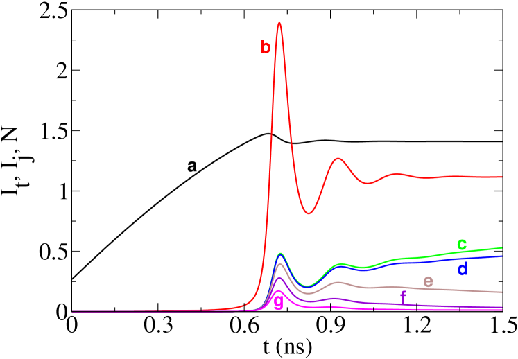
Figure 1: Time evolution of the total laser intensity, $I_{t}$ (curve (b)), following a sudden switch-on of the injected current (pump rate) in form of a Heaviside function centered at $t=0ns$. Initial current value: $J_{i}(t\leq 0^{-})=1.0mA$, final current value $J_{f}(t\geq 0^{+})=37.5mA$. The threshold current for this laser is $J_{th}=17.5mA$. Model with $M=113$ modes. All other parameters as in slowmodes . All parameter values are kept constant throughout the paper. With these values of $J_{i}$ and $J_{f}$ the intensity peak is reached at $t_{p}\approx 0.72ns$, while the steady state is attained at $\overline{t}\simeq 1.5ns$. Here and in all subsequent figures (unless otherwise specifically noted in the figure caption) the total intensity $I_{t}$ is divided by $2.5\times 10^{5}$, the individual mode intensities by $1\times 10^{5}$ and the carrier number $N$ is divided by $10^{8}$. Curve (a) shows the carrier number as a function of time. The other curves show the individual mode intensities for the central mode ($j=57$, (c)), and side modes close to line center (blue side): $j=56$ (d), $j=54$ (e), $j=52$ (f) and $j=50$ (g). The symmetric modes, relative to the central one, are not shown but are identical. Notice that in the first phases of the transient (peak) curves (c) and (d) are superposed on this scale: they separate only at the second oscillation.

III Analysis

The fast transient, leading to the intensity peak and the usual damped oscillations, can be divided into two parts. A first one, where the carrier number $N$ can be decoupled from the modal intensities $I_{j}$’s, and a second one where – due to the strong coupling – the fully nonlinear system must be retained.

In the decoupled regime, the carrier number plays the role of an energy reservoir, virtually unaffected by the presence of the laser modes (too weak to have an impact on the carriers). Thus, it is possible to find an analytical solution for its evolution – starting from an initial condition – towards a transient final state defined by the breakdown of this approximation (Section III.1). In this regime, the modal intensities are decoupled from one another (Section III.2) and evolve under the action of the (time-dependent) energy reservoir, $N$, whose behaviour has been analytically obtained with good accuracy in Section III.1. This approximate but accurate treatment allows us to define a “threshold” for the multimode laser (including spontaneous emission) in analogy with a basic single mode laser model, where spontaneous emission is traditionally neglected Narducci . The strongly coupled regime is analyzed in detail in Section III.3 on the basis of the knowledge acquired in Sections III.1 and III.2 and of ad hoc considerations.

The analysis of the fast transient is best conducted by choosing an initial state with the laser (almost) entirely off. A small amount of prebias ($J_{i}=1.0mA$, well below the lasing threshold initialbias which is placed around $J_{th}\approx 17.5mA$) is useful since it provides an average contribution of the spontaneous emission to each mode, without having to wait for the carrier number to grow. This choice is not restrictive and does not limit the validity of our results. Our analysis holds any time the laser starts from an injection current value below threshold, which corresponds to an initial energy repartition among modes which strongly differs from the final one, above threshold. If instead the laser is already pumped above threshold and we suddenly change its pump to another value above threshold dokhane2001 ; dokhane2004 , the ensuing dynamics will reflect the slow modal intensity redistribution examined in slowmodes .

III.1 Decoupled carrier dynamics

A good understanding of the initial phases of the laser turn-on requires a description, even though approximate, of its evolution away from noise. A good deal of work has been dedicated to an analytical or semi-analytical description of this question Petermann1978 ; Agarwal1993 ; Zhang2007 ; Ab-Rahman2010a ; Ab-Rahman2010b ; Ab-Rahman2011 ; Hisham2012 ; Sokolovskii2012 . In the following, we briefly outline the (standard) derivation of an approximate analytical solution for ease of comparison with the full, numerical integration of the model. The quantitative comparison will show that the analytical approximation provides excellent results even in the initial stages of the transient when the e.m. field intensity reaches relatively high values, i.e., exactly where one would expect the approximate solution to already fail.

The contribution of the spontaneous emission (intrinsic noise) to each mode is quite small. As a first approximation, we can therefore consider that the initial phases of the transient are well described by the set of eqs. (1) without the coupling term between individual modal intensities $I_{j}$ and carrier number $N$ in eq. (1b). In this approximation, we start by integrating the carrier number, eq. (1b), by variable separation:

$$\int_{N_{i}}^{\mathcal{N}}\frac{dN^{\prime}}{p(N^{\prime})} = \int_{0}^{t}dt^{\prime}\,,$$ (3)

where

$$p(N) = aN^{3}+bN^{2}+cN+d\,,$$ (4)

$$a = -C\,,$$ (5)

$$b = -(B+2CP_{0})\,,$$ (6)

$$c = -(A+BP_{0}+CP_{0}^{2})\,,$$ (7)

$$d = \frac{J}{q}\,,$$ (8)

with the constants given in slowmodes .

Formal integration of the left-hand-side (l.h.s.) of eq. (3) gives intwithmathematica

$$\int_{N_{i}}^{\mathcal{N}}\frac{dN^{\prime}}{p(N^{\prime})} = \sum_{\begin{array}[]{c}{\rm roots}\,\mu_{k}\\ {\rm of}\,p(N)\end{array}}\frac{\log(\mathcal{N}-\mu_{k})-\log(N_{i}-\mu_{k})}{3d\mu_{k}^{2}+2c\mu_{k}+b}\,.$$ (11)

With the parameter values of the problem, eqs. (5–8), only one root (which we will denote $\mu_{1}$) of $p(N)$ is real, while the other two are complex conjugate of each other

$$\mu_{3} = \mu_{2}^{\star}\,,$$ (12)

$$= \mathfrak{a}-i\mathfrak{b}\,.$$ (13)

Defining

$$z = \mathcal{N}-\mu_{2}\,,$$ (14)

$$z^{\star} = \mathcal{N}-\mu_{3}\,,$$ (15)

and equivalently for $z_{i}$, we expand the denominator of the formal solution (r.h.s. of eq. (11))

$$3d\mu_{k}^{2} +2c\mu_{k}+b=$$ (16)

$$[3d(\mathfrak{a}^{2}-\mathfrak{b}^{2})+2c\mathfrak{a}+b]\pm i[6d\mathfrak{a}\mathfrak{b}+2c\mathfrak{b}]\,,$$

$$\equiv \Omega_{r}\pm i\Omega_{i}\,,$$ (17)

$$k = 2,3$$ (18)

where the $+$ ($-$) sign in eqs. (16,17) corresponds to $k=2$ ($k=3$).

Thus, the contributions to eq. (11) coming from the two complex roots can be rewritten as

$$\sum_{\mu_{k},k=2,3} \frac{\log(\mathcal{N}-\mu_{k})-\log(N_{i}-\mu_{k})}{3d\mu_{k}^{2}+2c\mu_{k}+b}=$$ (19)

$$\left(\log(z)-\log(z_{i})\right)\frac{\Omega_{r}-i\Omega_{i}}{|\Omega|^{2}}+$$

$$\left(\log(z^{\star})-\log(z_{i}^{\star})\right)\frac{\Omega_{r}+i\Omega_{i}}{|\Omega|^{2}}\,,$$

with $z_{i}\equiv N_{i}-\mu_{2}$ (cf. eqs. (14,15)).

Substituting into the full expression, we finally obtain the solution for eq. (3):

$$t = \frac{\log(\mathcal{N}-\mu_{1})-\log(N_{i}-\mu_{1})}{3d\mu_{1}^{2}+2c\mu_{1}+b}+$$ (20)

$$2\left[\log|z|-\log|z_{i}|\right]\frac{\Omega_{r}}{|\Omega|^{2}}+$$

$$2\left[\operatorname{Arg}\left\{z\right\}-\operatorname{Arg}\left\{z_{i}\right\}\right]\frac{\Omega_{i}}{|\Omega|^{2}}\,.$$

This relationship implicitly defines the approximate solution for the carrier number and gives the most practical way of numerically representing the analytical solution: treating time as the dependent variable, $t(\mathcal{N})$, the function can be straightforwardly plotted (exchanging the horizontal and vertical axes allows one to restore the $\mathcal{N}(t)$ appearance of the function). Alternately, simple handling allows for a mathematical expression for $\mathcal{N}(t)$ which takes the form:

$$\left(\mathcal{N}(t)-\mu_{1}\right)\left(\mathcal{N}^{2}(t)-2\Re e\left\{\mu_{2}\right\}\mathcal{N}(t)+|\mu_{2}|^{2}\right)$$

$$\qquad\qquad e^{2\operatorname{Arg}\left\{\mathcal{N}(t)-\mu_{2}\right\}}=$$

$$\qquad\qquad\mathcal{K}e^{t}\,,$$ (21)

where

$$\mathcal{K} = \left(N_{i}-\mu_{1}\right)$$ (22)

$$\left(N_{i}^{2}-2\Re e\left\{\mu_{2}\right\}N_{i}+|\mu_{2}|^{2}\right)e^{2\operatorname{Arg}\left\{N_{i}-\mu_{2}\right\}}\,,$$

which can be used as an alternative definition of $\mathcal{N}(t)$ alt-def-N .

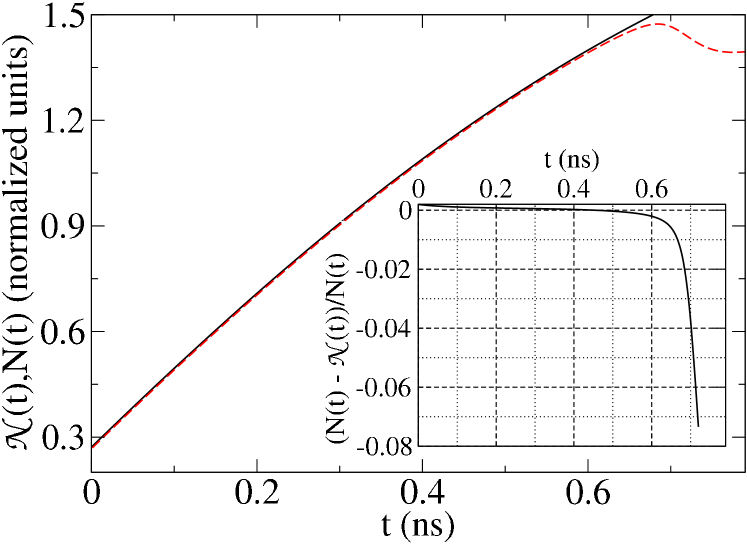
Figure 2: Comparison between the approximate analytical solution (solid line) $\mathcal{N}(t)$ and the complete carrier number (dashed line) $N(t)$ resulting from the integration of the full model, eqs. (1). The inset shows the difference between the full solution $N(t)$ and the analytical solution $\mathcal{N}(t)$ until the latter diverges away (at $t\approx 0.72ns$). Notice that even extremely near the intensity peak (cf. Fig. 1) the difference between the approximate and full solution remains modest ($\lesssim 8\%$).

Fig. 2 compares the analytical solution $\mathcal{N}(t)$ to the computed $N(t)$ obtained from the numerical integration of the full system, eqs. (1). The agreement between the approximate, analytical solution and the full integration is excellent up until values of time which are quite close to the intensity peak (occurring at $t\approx 0.72s$), as shown in the inset. The deviation is initially positive and remains below 0.5% (in absolute value) until $t\approx 0.62ns$. The initial positivity of the relative deviation,$\frac{N(t)-\mathcal{N}(t)}{N(t)}$, resides in the fact that the full solution requires a somewhat larger initial carrier number to support the different field modes, while in the approximate form no energy is lost to support them. The switch in sign in the difference between the exact and the approximate value for the carrier number comes from the fact that once the different lasing modes grow sufficiently large, the carrier number saturates, instead of continuing its growth, as in the approximate expression. The difference curve (inset) is numerically computed by integrating the full set of equations, eqs. (1), and a set equivalent to the analytical solution, obtained by removing from eq. (1b) the last term $\left(\sum_{j}\Gamma G_{j}(N)I_{j}\right)$ check-an-num .

Notice that at $t\equiv t_{th}\approx 0.62ns$, the carrier number $N(t)$ crosses its asymptotic value ($N(t_{th})=\overline{N}\equiv N(t\rightarrow\infty)$, cf. Fig. 1). In a laser model without spontaneous emission such a value would define the laser threshold, separating the decoupled dynamics for the population inversion (carrier number) from the strongly coupled regime (above threshold) Narducci . Here, this value sets the upper limit to the carrier number for which we can consider its dynamics decoupled from that of the modal intensities (when growing out of noise), thus we can extend the concept of “threshold” even in the presence of spontaneous emission.

III.2 Decoupled modal dynamics

We begin this section with an overview of the modal dynamics during the transient evolution, regardless of the degree of coupling with the carrier number. This allows us to get a general picture, which we then refine in the analysis of the decoupled regime (this section) and of the strongly coupled one (next section).

The individual mode traces in Fig. 1 show that at short times the lateral modes contribute more than their steady state share. Their peak (cf., e.g., curves (f) and (g) corresponding to modes 5 and 7 places away from line center) is much higher than the asymptotic intensity towards which they tend, contrary to those modes close to line center (for the central mode even the peak intensity is lower than its steady state value) slowmodes . This strongly suggests that a mechanism must exist for these modes to grow, in transient, well beyond their final value, while the very few central modes do not. Indeed, the accumulated intensity of the modes farthest away in the wings can exceed, in transient, that of the central mode, thus highlighting the impact that the side modes have on the initial phases of the dynamics.

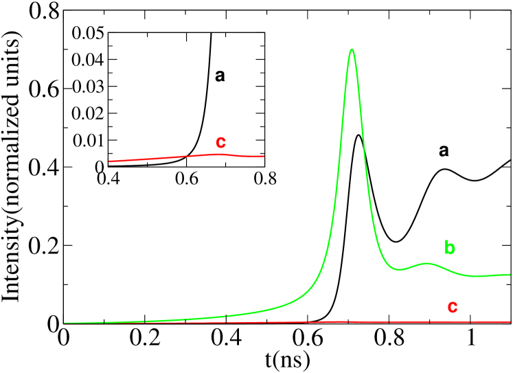
Figure 3: Temporal evolution of modes or groups of modes. Curve (a) traces the evolution of the central mode, (c) the sum of the most distant 20 modes on each side of line center, $I_{far}$, (cf. text for details) and (b) the sum of all side modes, $I_{M-17}$, save for those near line center (cf. text for details). The inset shows the initial phases of the transient and shows that the sum of the far modes (c) exceeds the intensity of the central mode (a) up until $t\approx t_{th}$.

A more complete illustration of this point is given by Fig. 3, which compares the time-dependent intensity of the central mode – curve (a) –, to the cumulative contribution of the most distant twenty modes (on each side, i.e. $I_{far}=\sum_{j=1}^{20}I_{j}+\sum_{j=94}^{113}I_{j}$) – curve (c)), and to that of all modes save for the 17 central ones (i.e.,$I_{M-17}=\sum_{j=1}^{48}I_{j}+\sum_{j=66}^{113}I_{j}$ – curve (b)).

The inset shows that below threshold $I_{far}$ (c) gives a contribution larger than that of the central mode (a) – until $t\lesssim 0.6ns$ – and that after a small maximum, at $t\approx 0.68ns$, it drops down again. Thus, the influence of the very far modes is of some importance only in the very first phases of the dynamics. Considering, though, that these modes are very far out in the wings and that their asymptotic value is order of magnitudes lower than that of the central mode, their strong influence on the dynamics up to threshold is an indicator of the essential difference between the transient intensity distribution and the asymptotic one!

The picture changes more dramatically if we include the lateral modes, $I_{M-17}$, which carry little energy at steady state (globally of the order of 3% of the total intensity), but which in transient give a cumulative peak larger than the one of the central mode (curve (b)). This contribution is rather striking. Indeed, it displays a faster growth than the central mode and deformed (incomplete) oscillations. The latter are explained by the fact that the effective relaxation frequency is not constant over the whole set of modes (cf. Marcuse1983 for discussion on a slightly different model and Section III.3, in this paper), thus the sum over the ensemble deforms and attenuates the oscillations.

The substantial contribution of $I_{M-17}$ to the peak in transient is a consequence of the observation that in the initial phases of the dynamics the lateral modes contribute, relatively, much more than they do at steady state (or at least on the long time scales). In addition, we remark that the anticipated peak for $I_{M-17}$ contributes to a faster growth of the total intensity. We now analyze the initial portion of the transient, i.e., the decoupled regime.

The remarks concerning the transient leading to, but excluding, the intensity peaks (and oscillations) can be better understood with the help of the following approximate analysis. Using the analytical (approximate) solution for $\mathcal{N}(t)$ (eq. (20)) we can now decouple the modal intensities to obtain an approximate dynamical evolution:

$$\frac{d\,{{}^{d}I_{j}}}{dt} \approx \left[\Gamma G_{j}(\mathcal{N})-\frac{1}{\tau_{p}}\right]{{}^{d}I_{j}}+$$ (23)

$$\beta_{j}B\mathcal{N}(t)\left[\mathcal{N}(t)+P_{0}\right]\,,$$

where the superscript ^d denotes the approximate, decoupled variable.

The following auxiliary quantities simplify the notations:

$$\alpha_{j} = \Gamma g_{p}\left[1-2\left(\frac{\lambda_{j}-\lambda_{p}}{\Delta\lambda_{G}}\right)^{2}\right]\,,$$ (24a)

$$\mathcal{K}_{j} = \alpha_{j}N_{0}+\frac{1}{\tau_{p}}\,,$$ (24b)

$$B_{j} = \beta_{j}B\,,$$ (24c)

where we have neglected the saturation term $\epsilon I_{t}$ in the expression for $G_{j}(N)$, eq. (2), since we are examining the transient portions in which the intensity is very small, $\epsilon$ being also very small (cf. Table III in slowmodes ). This way, the modal intensities obey the set of M decoupled ODEs

$$\frac{d\,{{}^{d}I_{j}}}{dt} \approx \left[\alpha_{j}\mathcal{N}(t)-\mathcal{K}_{j}\right]{{}^{d}I_{j}}+B_{j}\mathcal{N}(t)\left[\mathcal{N}(t)+P_{0}\right]\,,$$ (25)

which can be globally analyzed.

Over very short time intervals $\Delta t$ ($\Delta t$: $\mathcal{N}(t+\Delta t)\approx\mathcal{N}(t)$, $\forall\,t:$ ($0\leq t\lesssim t_{th}$) ) we can consider the two terms $\left[\alpha_{j}\mathcal{N}(t)-\mathcal{K}_{j}\right]$ and $B_{j}\mathcal{N}(t)\left[\mathcal{N}(t)+P_{0}\right]$ as being constants, thus reducing eq. (25) to an ensemble of ODEs with constant coefficients. In such a case, formal integration provides immediately a solution for the approximate problem, eq. (25):

$${}^{d}I_{j}(t_{k}+t^{\prime}) \approx -\frac{B_{j}\mathcal{N}(t_{k})\left[\mathcal{N}(t_{k})+P_{0}\right]}{\alpha_{j}\mathcal{N}(t_{k})-\mathcal{K}_{j}}+$$ (27)

$$\left[{{}^{d}I_{j}(t_{k})}+\frac{B_{j}\mathcal{N}(t_{k})\left[\mathcal{N}(t_{k})+P_{0}\right]}{\alpha_{j}\mathcal{N}(t_{k})-\mathcal{K}_{j}}\right]$$

$$e^{\left[\alpha_{j}\mathcal{N}(t_{k})-\mathcal{K}_{j}\right]t^{\prime}}\,,$$

$$= -\frac{\mathcal{B}_{j}(t_{k})}{\gamma_{j}(t_{k})}+$$

$$\left[{{}^{d}I_{j}(t_{k})}+\frac{\mathcal{B}_{j}(t_{k})}{\gamma_{j}(t_{k})}\right]e^{\gamma_{j}(t_{k})\cdot t^{\prime}}\,,$$

$$\gamma_{j}(t_{k}) \equiv \alpha_{j}\mathcal{N}(t_{k})-\mathcal{K}_{j}\quad(<0)\,,$$ (28)

$$\mathcal{B}_{j}(t_{k}) \equiv B_{j}\mathcal{N}(t_{k})\left[\mathcal{N}(t_{k})+P_{0}\right]\,,$$ (29)

$$t_{k} \equiv k\times\Delta t\,,$$ (30)

$$k = 0\ldots q\,,$$ (31)

$$0\leq t^{\prime} \leq\Delta t\,,$$ (32)

$${{}^{d}I_{j}(t_{0})} = I_{j}(t_{0})\,,$$ (33)

are the initial conditions for each modal intensity. The inequality in parenthesis (eq. (28)) holds strictly in the range of validity of the current approximation. Here $t^{\prime}$ is a local time defined in each interval $\Delta t$ and is zeroed at the beginning of each time step.

The coefficients $\mathcal{B}_{j}(t_{k})$ and $\gamma_{j}(t_{k})$ diff-gamma-beta are constant over a small time interval $\Delta t$ and are “updated”, as time evolves, at the next value $t_{k}$. This, in itself, is not a limitation since their functional dependence is known and explicitly given by eqs. (21,22,24). Thus, eq. (27) is a “piecewise”, recursive solution over a discrete ensemble of times $t_{k}$ ($k=0\ldots q\,:t_{0}=0,t_{q}\approx t_{th}$). At each time step, each ${}^{d}I_{j}$ starts to converge, for a short time, towards its locally asymptotic solution before being updated to the next time step. The form of the approximate solution, eq. (27), highlights the role of the different coefficients: the spontaneous emission term, $\mathcal{B}_{j}$, controls the amplitude (together with $\gamma_{j}$ in the prefactor of eq. (27)), while gain, $\alpha_{j}$, and cavity losses, $\mathcal{K}_{j}$, combined into $\gamma_{j}$ play the role of an effective relaxation constant. Notice that $\gamma_{j}$ results from the composition, eq. (28), of the two functions shown in the inset of Fig. 4 (notice the shift and multiplicative factor for curve B – cf. figure caption) which represent $\alpha_{j}$ (curve A) and $\mathcal{K}_{j}$ (curve B). The different local curvatures, combined with the multiplication of curve A by the carrier number $N(t)$ (or equivalently $\mathcal{N}(t)$ when using the approximate solution), differentiate the coefficient $\gamma_{j}$ for the individual modes (with the possibility of obtaining, in transient, positive values when curve A$\times N$ is larger than curve B – possible only outside the range of validity of the current approximation).

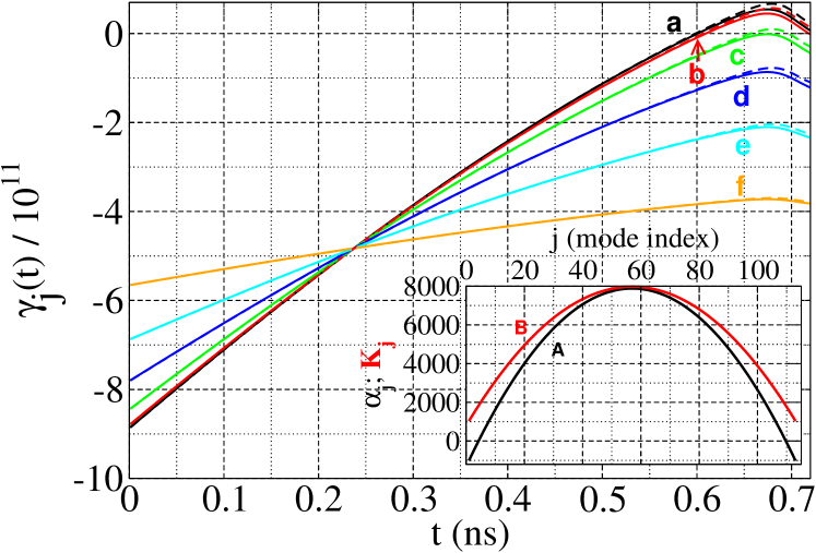
Figure 4: Time evolution of $\gamma_{j}$ (in units of $10^{11}$) for selected modes: (a) j = 57; (b) j = 50; (c) j = 40; (d) j = 30; (e) j = 20; (f) j = 10. The solid lines correspond to the values of $\gamma_{j}$ computed from the full set of equations, eqs. (1), while the dashed lines (which separate only for $t>t_{th}$ from the solid lines) are computed for the analytical solution $\mathcal{N}(t)$, eq. (21,22). The inset shows the modal dependence of $\alpha_{j}$ (curve (A)) and $\mathcal{K}_{j}$ (curve (B)). For graphical purposes we have plotted instead of $\mathcal{K}_{j}$ its normalized and shifted version K${}_{j}=\frac{\mathcal{K}_{j}}{1\times 10^{8}}-3\times 10^{3}$.

In order to better understand the behaviour of this approximate solution, we trace the coefficients $\gamma_{j}$ and $\mathcal{B}_{j}$ for selected modes in Figs. 4 and 5, respectively. Fig. 4 shows the evolution of $\gamma_{j}$ as a function of time for a representative sample of modes. Aside from the initial portions of the transient transp ($t\lesssim 0.24ns$) the larger $\gamma_{j}$, the closer is the corresponding mode to line center. Since $\gamma_{j}$’s behave as effective relaxation constants, the figure immediately shows that the wing modes, with their larger (negative) values of $\gamma$, react on a shorter time scale than those modes close to line center. This explains the numerical observation of Fig. 3, where the wing modes grow faster than the central one, and partly accounts for the excess growth of these modes beyond their asymptotic values constr-bth . The constraint which forces the energy to be distributed over all modes (cf. discussion in Section IVA of slowmodes ), transfers the excess which cannot be taken up by the stronger (and slower) modes to the faster wing modes during the transient. On the longer time scales, on which the central mode(s) react(s), the energy is transferred back, allowing the side modes to relax to their asymptotic values. Notice that the agreement between the coefficients calculated from the analytical solution for the carrier number and from the full numerical solution holds extremely well until after threshold: in Figs. 4 and 5 one can distinguish solid and dashed curves only in the top right hand portion of the figure.

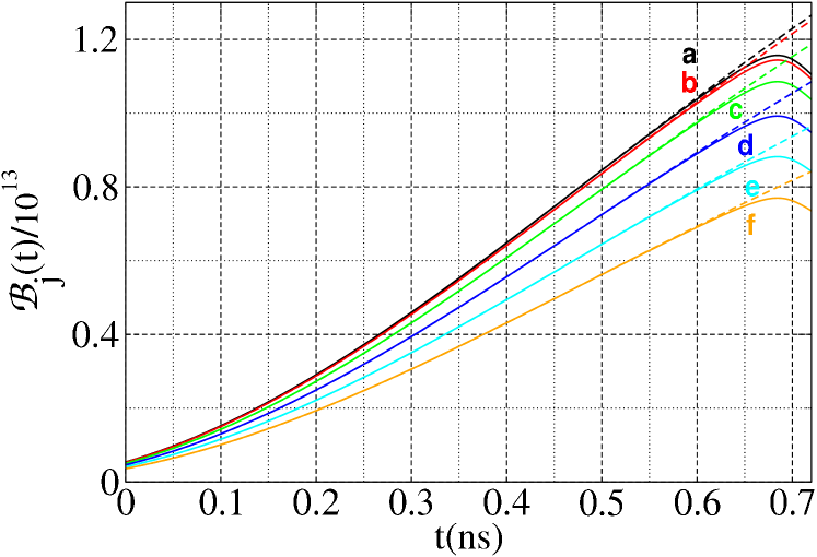
Figure 5: Time evolution of the spontaneous emission contribution to each individual mode (in units of $10^{13}$) for selected modes: (a) j = 57; (b) j = 50; (c) j = 40; (d) j = 30; (e) j = 20; (f) j = 10. The solid lines correspond to the values of $\beta_{j}N(t)\left[N(t)+P_{0}\right]$ computed from the full set of equations, eqs. (1), while the dashed lines (which separate only for $t>t_{th}$ from the solid lines) are computed for the analytical solution $\mathcal{N}(t)$ in place of $N(t)$, eq. (21,22). The labels (a) and (b) correspond, from top to bottom, to the top two sets of curves (solid and dashed, respectively) which can be distinguished only on the far right of the figure.

In addition to the component ($\gamma_{j}\,{{}^{d}I_{j}}$ in eq. (25), with the substitutions, eqs. (28,29)) discussed so far, the temporal evolution of the individual modes includes the contribution of the spontaneous emission $\mathcal{B}_{j}$ whose amplitude is plotted in Fig. 5 (dashed lines) for a subset of modes, as a function of time (thus, of carrier number, cf. eq. (20)) and is compared to the amplitude (solid lines) for the full model, eqs. (1). Its main feature is the similarity in its contribution to all modes (maximum deviation, less than a factor 2) even at the end of the time interval (largest $\mathcal{N}(t)$). The bundle of curves opens up with time, increasing by about one order of magnitude for the central mode ($j=57$) – somewhat less for the plotted mode farthest away from line center ($j=10$). For the latter mode we remark that $\frac{\gamma_{10}(t_{th})}{\gamma_{10}(0)}\approx\frac{2}{3}$, thus maintaining a nearly constant, fast relaxation throughout the decoupled regime. The fast, nearly constant, reaction time explains the sizeable growth of the wing modes, in spite of the smaller contribution which they receive from the spontaneous emission. The moderate change in $\gamma_{10}$ (and equivalent from the wing modes) ensures a slight growth in the prefactor of eq. (27), thus a rather stable energy contribution of these modes below threshold. For comparison, in the units of Fig. 4, $\gamma_{57}(t\rightarrow\infty)\approx-10^{-3}$ (cf. slowmodes ). Hence, the effective relaxation rate changes considerably for the center mode and is eventually responsible for their predominance at the end of the below-threshold regime, even though the side modes maintain a level which is considerably larger than their asymptotic contribution.

The approximate solution, eq. (27), shows the role played by $\frac{\mathcal{B}_{j}(t_{k})}{\gamma_{j}(t_{k})}$, which is nothing else than the ratio between the coefficients shown in Figs. 4,5. Thus, another way of interpreting the dynamics below threshold is to plot, Fig. 6, the r.h.s. of eq. (25) – thus the intensity increment – for the whole ensemble of modes at selected times (i.e., for selected values of $\mathcal{N}(t)$), from the initial condition up to threshold.

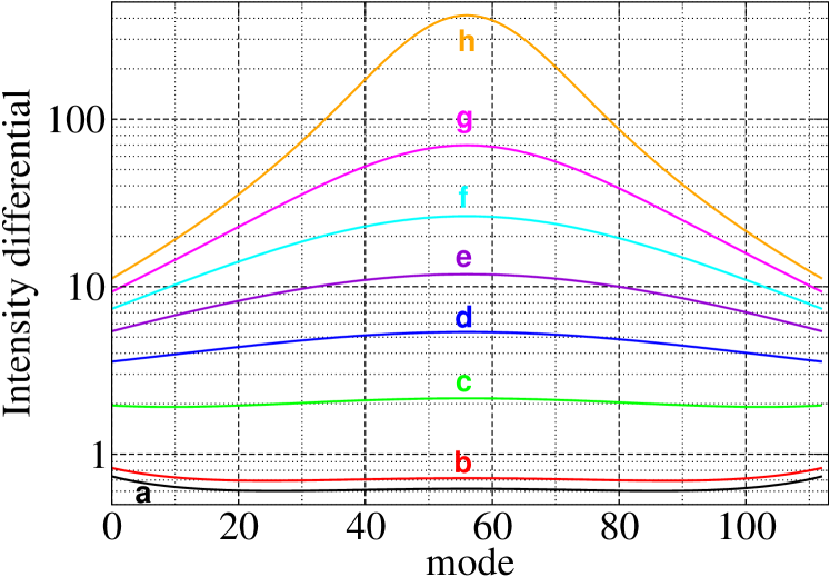
Figure 6: Differential increment (numerically computed with a time step $\Delta t=1\times 10^{-14}s$) for the individual mode intensities (r.h.s. of eq. (25)) plotted at different times: (a) $t=0.001ns$ ($\mathcal{N}=2.17558\times 10^{7}$); (b) $t=0.01ns$ ($\mathcal{N}=2.893353\times 10^{7}$); (c) $t=0.1ns$ ($\mathcal{N}=4.903313\times 10^{7}$); (d) $t=0.2ns$ ($\mathcal{N}=7.033165\times 10^{7}$); (e) $t=0.3ns$ ($\mathcal{N}=9.024550\times 10^{7}$); (f) $t=0.4ns$ ($\mathcal{N}=1.085107\times 10^{8}$); (g) $t=0.5ns$ ($\mathcal{N}=1.249524\times 10^{8}$); (h) $t=0.6ns$ ($\mathcal{N}=1.394853\times 10^{8}$).

When the carrier number is well below transparency (curves a-c) the gain is nearly equal for all modes, with a somewhat higher level in the wings for the first two curves winggain . This implies that the modes far from line center start growing faster than the central ones. Near transparency, curve (d), the central modes start dominating and the combined effect of their somewhat larger intensity and of their increasing coefficients (cf. Figs. 4,5) favors them. For the parameters of curve (e) the laser is already beyond transparency ($N_{0}=7.8\times 10^{7}$, $t\approx 0.24ns$) and the tendency for a strong differential growth becomes obvious and sharpens itself with growing values of $\mathcal{N}$. Equivalent curves showing the ratio (cf. eq. (27)) $\frac{\mathcal{B}_{j}}{\gamma_{j}}$ (each component plotted in Figs. 4,5) look qualitatively very similar to those of Fig. 6, since they differ only for the intensity ${}^{d}I_{j}$ which multiplies $\gamma_{j}$ (the relative deformation is most visible for curve (h), which is more strongly reshaped by the larger modal intensity variations).

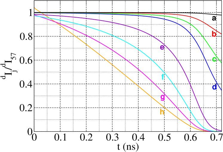
Figure 7: Intensity ratio $\frac{{}^{d}I_{j}}{{}^{d}I_{57}}$ for a selected subset of modes: (a) $j=56$; (b) $j=54$; (c) $j=52$; (d) $j=50$; (e) $j=40$; (f) $j=30$; (g) $j=20$; (h) $j=10$. The ratios are computed with the decoupled system of equations, eqs. (20,25).

In spite of the clear increase in differential intensity growth between the central and the side modes displayed in Fig. 6 the ratio remains finite up until threshold, as shown in Fig. 7, where the amplitude of each intensity mode is displayed normalized to the intensity of the central mode. Fig. 7 shows again that the gain is largest for the wing modes at the start of the transient (curve (h), $j=10$, is the highest at $t=0$), due to their lower absorption and that during the whole evolution in the decoupled regime the relative weight of the side modes largely exceeds their asymptotic value $\left(\left.\frac{{}^{d}I_{10}}{{}^{d}I_{57}}\right|_{t\approx 0.6ns}\approx 0.05\right.$ – cf. Fig. 7 – to be compared to $\frac{\overline{I}_{10}}{\overline{I}_{57}}\approx 1.5\times 10^{-4}$ from Table 1). This result is consistent with the numerical observation – obtained from the integration of the full model, eqs. (1) – showing that at $t=0.6ns$ the cumulative intensity of the 20 modes farthest away from line center, $I_{far}$, exceeds that of the central mode (cf. Fig. 3). It also explains why at $t=\overline{t}$ the intensity distribution is far from the asymptotic one (Fig. 1 and slowmodes ): the wing modes at the beginning of the strongly coupled regime hold a very large relative amount of energy ($\approx$ 300 times its relative asymptotic value for $j=10$).

Besides the numerical evidence of Fig. 7, eq. (27) shows the reason for the not-so-large differences among modes, below threshold. Expanding the exponential in eq. (27) to first order, we obtain an approximate form for the modal intensity:

$${}^{d}I_{j}(t_{k}+t^{\prime}) \approx {{}^{d}I_{j}(t_{k})}\left[1+\gamma_{j}(t_{k})\cdot t^{\prime}\right]+\mathcal{B}_{j}(t_{k})\cdot t^{\prime}\,,$$ (34)

thus its increment relative to the previous time step takes the form:

$${}^{d}I_{j}(t_{k}+t^{\prime})-{{}^{d}I_{j}(t_{k})} \approx {{}^{d}I_{j}(t_{k})}\gamma_{j}(t_{k})\cdot t^{\prime}+$$ (35)

$$\mathcal{B}_{j}(t_{k})\cdot t^{\prime}\,.$$

The first term on the r.h.s. of eq. (35) represents a relaxation ($\gamma_{j}<0$, $\forall(j,t_{k})$), while the second one is the modal intensity increment brought about by the (average) spontaneous emission contribution. Thus, the differential growth between center and wing modes remains moderate (cf. Fig. 5), which explains why even close to threshold the ratio of the wing modes to the center mode (Fig. 7) remains very large compared to its asymptotic value. Notice that eq. (35) indirectly determines a time step $\Delta t$, since $\Delta t\ll\frac{1}{\mathcal{B}_{j}(t_{k})}$, $\forall(j,t_{k})$ convergence-radius .

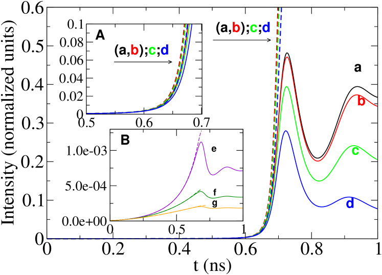
Figure 8: Temporal evolution of the intensity for a selected subset of modes: (a) $j=57$; (b) $j=56$; (c) $j=54$; (d) $j=52$; (e) $j=30$; (f) $j=20$; (g) $j=10$. The solid lines display the result of the integration of the full model, eqs. (1), while the dashed lines show, for comparison, the corresponding intensity values calculated from the decoupled model (eqs. (20,25)). Inset A shows a detail of the temporal evolution around $t_{th}$ to see how the approximate and the full solution deviate from each other. Inset B shows three selected wing modes. Values for the intensity peaks and corresponding times are given in Table 1. Notice that in the main figure, as well as in inset A, curves (a) and (b) are practically indistinguishable. The arrow underneath the label in these two figures shows the order in which the labels have to be attributed to the (closely) adjacent curves.

Fig. 8 shows the temporal evolution of a selection of modes (those close to line center) for the full integration (eqs. (1), solid lines) and for the decoupled system (eqs. (20,25), dashed lines). We notice that over the whole range of validity ($t\leq t_{th}$) of the analytical solution for the carrier number, eq. (20), the decoupled approximation is very good. Inset A shows a detail of the temporal evolution for the same modes close to threshold: all curves lie extremely close to one another, confirming the validity of our approximation. Inset B shows the evolution for three wing modes (cf. caption): the agreement between full solutions (solid lines) and analytical approximations (dashed lines) remains excellent even beyond threshold for these modes.

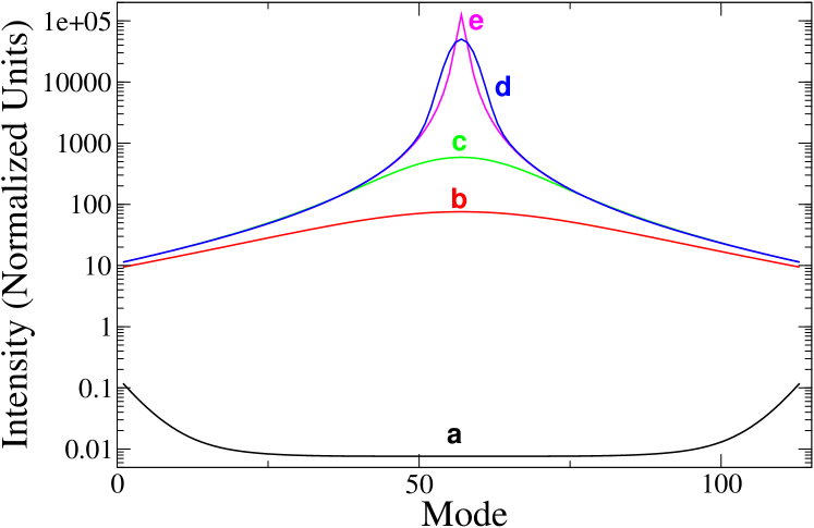
Figure 9: Intensity distribution for all modes considered in the integration, each curve corresponding to a different time: (a) initial condition; (b) $t=0.62ns$ (threshold crossing); (c) $t=0.726ns$ (total intensity peak); (d) $t=1.5ns$ (total intensity and carrier density relaxed to their asymptotic value): beginning of the slow transient slowmodes ; (e) $t=35ns$ (asymptotic intensity distribution). The intensity values are plotted in logarithmic scale and are not rescaled according to the factors specified in Fig. 1.

We summarize the main result of this section in Fig. 9 which shows how the intensity distribution among all modes at the end of the decoupled regime (i.e., the instant when the population carrier crosses its asymptotic value – threshold – for the first time) does not differ very substantially from the initial distribution. Curve a (black online) shows the equilibrium intensity distribution at the initial condition – the side modes carry more intensity thanks to their reduced absorption (below transparency). Curve b (red online) shows the intensity distribution at threshold (cf. above) – i.e., $t\approx 0.62ns$. Even though the central modes carry a larger amount of intensity (and the shape of the curve is inverted, compared to the initial condition, when comparing to the asymptotic, equilibrium, distribution (curve d, blue online), the quantitative differences among modes at the first threshold crossing are nearly negligible. Anticipating on the next section, we remark that even at the peak in the total intensity the intensity distribution among modes (curve c, green online) differs less from the threshold condition than from the asymptotic one.

In conclusion, in this section we have shown that the decoupled model gives a very good representation of the evolution of the modal content of the laser output in the below threshold region, i.e., over a large part of the transient. We have also seen, both numerically and analytically, how the side modes carry an amount of energy much larger than their asymptotic share. Once the system overcomes this threshold, the analytic approximation for the carrier number breaks down, the coupling becomes strong and only the full numerical solution can account for the remainder of the fast evolution towards the steady state for the two global variables ($N$, and $I_{t}$ slowmodes ).

III.3 Strongly coupled regime

The two preceding sections have analyzed in detail the portion of the dynamical evolution below the threshold value for the carrier number. Here we are going to investigate the next portion of the dynamics def-linear-regime , which corresponds to the full nonlinear coupling between modes and which leads, eventually, into the time-independent total intensity with the residual slow evolution of the modal intensity distribution slowmodes . Our analysis of the multimode high-intensity regime is based on a direct integration of the model equations and on the potential for the interpretation of the resulting observations which comes directly from the detailed analysis of the previous sections. A direct-solution approach, such as the one adopted in Demokan1984 for an analytical construction of the solution for short pulses in a single-mode device, would be very hard to adopt in our strongly multimode model.

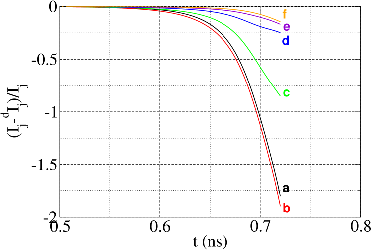
Figure 10: Relative deviation between the full-dynamics and the decoupled dynamics $\left(\frac{I_{j}-^{d}I_{j}}{I_{j}}\right)$ and onset of the strongly-coupled regime. (a) total intensity; (b) $j=57$; (c) $j=40$; (d) $j=30$; (e) $j=20$; (f) $j=10$;

Fig. 10 clearly shows the transition between the decoupled regime, where the deviation between the approximate and exact modal intensities is at most 5% (at $t\approx 0.6ns$), and the fully nonlinear regime, where this difference rapidly diverges. The transition is clearly illustrated by Fig. 4 which shows that during their growth some $\gamma_{j}$’s become positive for a subensemble of modes (near line center) and oscillate together with the carrier number to relax slowmodes to their (negative asympt-gamma ) asymptotic values (not shown). When some $\gamma_{j}>0$ the nature of eq. (27) changes, since the growth of the ${}^{d}I_{j}$’s is no longer exclusively due to the growth of the prefactor but also to the exponential growth of (some) ${}^{d}I_{j}$’s, which eventually leads to a divergence from the solution of the full model, eqs. (1).

From the point of view of the solution of eqs. (1) the positivity of some $\gamma_{j}$’s bears no weight. Indeed, throughout the growth of the modal intensities ($t\leq 0.72ns$, cf. Fig. 1), the r.h.s. of eq. (1a) (or, equivalently, eq. (23)) remains positive due to the contribution of the spontaneous emission ($\mathcal{B}_{j}$), independently on the sign of $\gamma_{j}$. Thus, the latter contributes quantitatively, but not qualitatively, to the growth of the modal intensities ${}^{d}I_{j}$.

Table 1: Intensity value at the first$(n=1)$ and second $(n=2)$ peak, ${}^{pn}I_{j}$, and time of occurrence, ${}^{pn}t_{j}$, ${}^{p1,p2}\Delta t_{j}\equiv{{}^{p2}t_{j}}-{{}^{p1}t_{j}}$ time difference between the peaks, and asymptotic intensity $\overline{I}_{j}$ for each laser mode $j$ (from the full set of equations, (1)). The last line, separated from the rest of the table, gives the equivalent information for the total intensity.

Mode	${}^{p1}I_{j}$	${}^{p1}t_{j}(ns)$	${}^{p2}I_{j}$	${}^{p2}t_{j}(ns)$	${{}^{p1,p2}\Delta t_{j}}(ns)$	$\overline{I}_{j}$
57	48182	.7140	39449	.9264	.2124	125645
56	47111	.7138	37299	.9248	.2110	41210
55	44054	.7134	31598	.9210	.2076	13627
54	39443	.7126	24136	.9152	.2026	6437
52	27972	.7102	10805	.9010	.1908	2387
50	17190	.7070	3856	.8858	.1788	1223
40	717	.6854	229	.8786	.1932	198
30	112	.6726	76	.8682	.1956	72
20	42	.6700	35	.8670	.1970	34
10	21	.6718	18	.8694	.1976	18
tot	598171	.7100	317103	.9147	.2047	279118

A closer look at the modal dynamics (solid lines in Fig. 8) shows that all individual modes display the same generic behaviour (peak with damped oscillations) but that some differences appear in the time at which the peaks occur and in the shape (frequency and damping) of the oscillations. Table 1 gives the time ${}^{p_{1}}t_{j}$ at which the intensity maximum (${}^{p_{1}}I_{j}$) is reached for a selection of modes. A clear anticipation in the first peak appears as the mode index moves away from line center ($j=57$), not unexpectedly after the discussion of the previous section based on the behaviour of the $\gamma_{j}$’s (Fig. 4). An inversion in this tendency, however, appears comparing ${}^{p_{1}}t_{20}$ and ${}^{p_{1}}t_{10}$, hinting to a more complex behaviour in the strong-coupling regime.

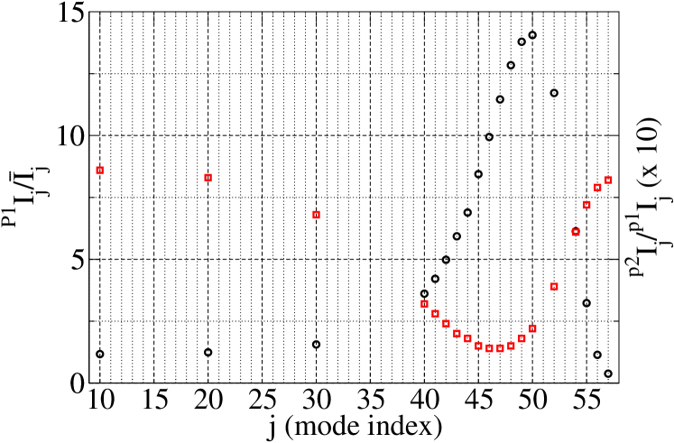
Figure 11: Modal peak amplitude relative to the modal steady state, $\frac{{}^{p_{1}}I_{j}}{\overline{I}_{j}}$ (circles, left scale) and amplitude of the second peak relative to the first peak, $\frac{{}^{p_{2}}I_{j}}{{}^{p_{1}}I_{j}}$ (squares, right scale) for a selection of laser modes. Notice that the central mode is at the far right, thus for picturing the full set of modes one should mirror-image the figure with respect to vertical axis passing through $j=57$. For the total intensity, the equivalent quantities are (from Table 1): $\frac{{}^{p1}I_{tot}}{\overline{I}_{tot}}=2.14$, $\frac{{}^{p2}I_{tot}}{{}^{p1}I_{tot}}=0.53$.

Fig. 11 shows the ratio between the maximum peak amplitude for each mode and its corresponding asymptotic value (circles, left scale). For the central mode the peak amplitude ${}^{p1}I_{57}$ is about half its steady state, $\overline{I}_{57}$, while in the far wings the peak (e.g., ${}^{p1}I_{10}$) is only slightly higher than its steady state ($\overline{I}_{10}$), showing that equilibrium for these modes is reached rather smoothly (i.e., with little overshoot and oscillations). However, the peak amplitude grows very large for modes off line-center, but not too far from it, the largest ratio occurring for $j=50$ (six places away from line center) whose peak intensity ${}^{p_{1}}I_{50}\approx 14\times\overline{I}_{50}$. This highlights the role of the (close) side modes in the strongly coupled regime, which temporarily carry a large amount of energy.

Associated with this strong variation in the peak intensity, a remarkable, nearly anti-correlated, variation in the damping appears. The ratio between the second and the first peak $\left(\frac{{}^{p_{2}}I_{j}}{{}^{p_{1}}I_{j}}\right)$ is represented by squares (Fig. 11, right scale)). While at line center and far off in the wings the second peak is almost as large as the first ($\gtrsim 80\%$), for the strongest overshoot we notice (almost) the largest damping (with a slight shift, $\frac{{}^{p_{2}}I_{47}}{{}^{p_{1}}I_{47}}\approx 0.2$).

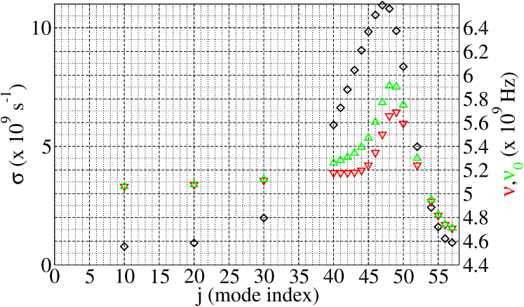
Figure 12: Modal damping coefficient, $\sigma_{j}$ (diamonds, left scale), modal damped (down-triangles), $\nu_{j}$, and undamped (up-triangles), $\nu_{0,j}$, relaxation oscillation frequency (right scale). Notice that the central mode is at the far right, thus for picturing the full set of modes one should mirror-image the figure with respect to vertical axis passing through $j=57$. The equivalent quantities for the total intensity are: $\sigma_{tot}=3.10\times 10^{9}s^{-1}$, $\nu_{tot}=4.885GHz$, $\nu_{0,tot}=4.910GHz$.

Assuming a simple dependence for the damped oscillations, of the form $I_{j}(t)=I_{0,j}e^{-(\sigma_{j}+i2\pi\nu_{j})t}$, we can estimate the modal damping constant $\sigma_{j}$ in the strongly coupled regime, together with the oscillation frequency $\nu_{j}$ directly from the data, using the peak amplitudes (${}^{p_{1}}I_{j}$, ${}^{p_{2}}I_{j}$) and times (${}^{p_{1},p_{2}}\Delta t_{j}\equiv{{}^{p_{2}}t_{j}}-{{}^{p_{1}}t_{j}}$) at which they occur. With the help of the standard expression for the undamped frequency $\nu_{0}$ of a damped oscillator, we can further estimate $\nu_{0,j}=\sqrt{\left(\frac{\sigma_{j}}{2\pi}\right)^{2}+\nu_{j}^{2}}$. The corresponding results are shown in Fig. 12 for the damping $\sigma_{j}$ (diamonds, left scale) and for the damped (down-triangles), $\nu_{j}$, and undamped (up-triangles), $\nu_{0,j}$, frequencies (right scale for both).

A resonance-like behaviour appears clearly in the relaxation oscillation frequency, with a maximum at mode $j=48$ for $\nu_{0}$ (at $j=49$ for $\nu$), and a sizeable variation in frequency $\Delta\nu_{0}=\nu_{48}-\nu_{57}\approx 1.2GHz$ (i.e., $\frac{\Delta\nu_{0}}{\nu_{57}}\approx 25\%$). The contribution due to the modal damping $\sigma_{j}$ is clearly visible in the graph and increases the frequency, at its maximum, by $\frac{\nu_{0,48}-\nu_{48}}{\nu_{48}}\approx 4\%$, while shifting it away from line center (by one mode). The combination of the contribution of all modes lends the total intensity (Fig. 1) features (cf. captions of Figs. 11, 12) which are a combination of those of different modes. Looking at the damping, $\sigma_{tot}$ or at the relative height of the first peak, $\frac{{}^{p1}I_{tot}}{\overline{I}_{tot}}$, the values are similar to those of mode $j=53$, the relaxation oscillation frequencies, $\nu_{tot},\nu_{0,tot}$, are consistent with mode $j=54$, while the second peak is less strongly damped, as for a mode placed between $j=55$ and $j=56$.

We therefore conclude that the dynamics in the portion of the fast transient corresponding to the strongly-coupled regime is dominated by a group of modes close to, but not at, line-center.

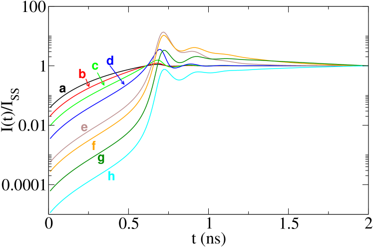
Figure 13: Temporal evolution for a sample of modes normalized to their individual asymptotic intensity values. To simplify the label, we have omitted the subscript $j$ for the variable $I$ in both numerator and denominator of the vertical axis. (a) $j=10$; (b) $j=20$; (c) $j=30$; (d) $j=40$; (e) $j=50$; (f) $j=52$; (g) $j=54$; (h) $j=57$. Mode $j=56$ shows the same evolution as mode $j=57$ (in this figure) slightly displaced towards higher values (not shown for simplicity).

An equivalent graphical illustration is given by Fig. 13 which shows the transient evolution for each mode, normalized to its asymptotic value. The modes far in the wings show a very early and gradual growth with little overshoot and oscillations (the decay is masked by the normalization to their asymptotic state, cf. slowmodes ). Coming closer to line center we notice a gradual delay in the growth, accompanied by a sharp, and very large, peak and a gradual relaxation towards the asymptotic intensity level. The last mode to grow is the central one, whose peak, together with the first side mode, is lower than its steady state. The relaxation for the central modes is extremely slow and extends well beyond the figure range slowmodes .

Fig. 13, together with the analysis of the previous sections, convincingly demonstrates the reason for the slow dynamics discussed in slowmodes . The transient evolution from the initial, below-threshold condition takes place first through a regime where the modal growth is not strongly differentiated between mode center and wings (i.e., below threshold). When the laser finally passes threshold, the central (slower) modes have to grow away from an intensity distribution which is far from the asymptotic one (Fig. 9). This intensity configuration favours those lateral modes which are sufficiently close to line center to have a strong growth, but which at the same time possess faster time constants, which allow them to more rapidly exploit the excess population inversion. Thus, we find a strongly out-of-equilibrium intensity distribution at the peak (curve c in Fig. 9), and it is not surprising that when the total intensity and the carrier number have relaxed to their respective asymptotic values (at $t\approx 1.5ns$ for the initial conditions chosen in this paper, Fig. 1) the modal repartition of the intensity be still strongly very far from its asymptotic configuration. In this way, we clearly understand the reason for the slow dynamics reported in slowmodes .

IV Transient spectra

The analytical and numerical treatment of the transient has given us a good description of the modal evolution from the initial state (laser – nearly – off) to the point where the two global variables ($N$ and $I_{t}$) have attained equilibrium. We now look at the time-resolved transient emission spectrum, defined as the frequency interval over which the modal intensity passes a chosen percentage of the total output intensity, $W^{FS}_{x}$, where $FS$ stands for Full Spectral and $W$ for Width, while $x$ fixes the chosen level in dB. We remark that, contrary to what found for the slow dynamics slowmodes , the transient spectra are only marginally affected by the modal arrangement under the gain line (even vs. odd number of modes in the simulation – cf. slowmodes for a discussion). We will therefore discuss only the modal placement used so far.

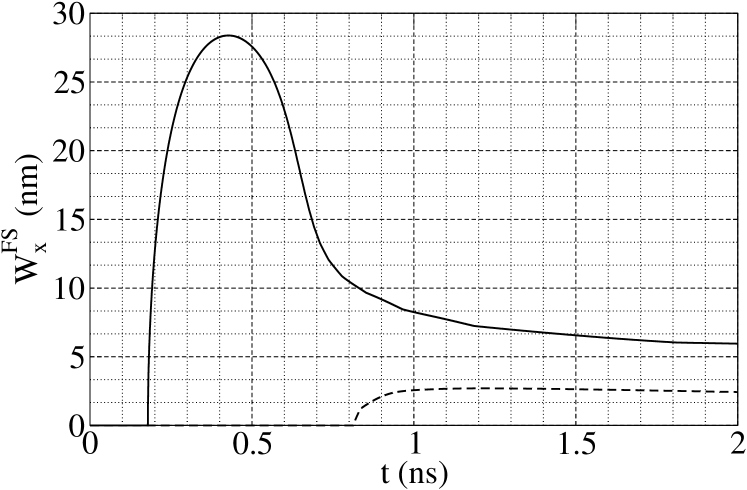
Figure 14: Full spectral width $W^{FS}_{x}$ of the laser evolution during the transient. Solid lines $x=40dB$, dashed lines $x=20dB$. The level in $dB$ is defined, as in slowmodes , as the modal intensity which passes the preset level compared to the instantaneous total intensity.

Fig. 14 shows the Full Spectral Width ($W^{FS}$), resolved in time, calculated at -40 dB ($W^{FS}_{40}$, solid line) and at -20 dB ($W^{FS}_{20}$, dashed line). The frequency “edge”, marked by each line in the figure, is obtained by linear interpolation between the frequencies of the two modes between which the $W^{FS}_{x}$ criterion is satisfied. The -40 dB level captures the full evolution of the spectral content during the transient; we recognize that in the very first phases of the transient ($<0.2ns$) none of the modes passes this mark (the spectral width starts at this point) farbelow because the intensity is widely distributed over a large number of modes, rather than being carried by a few modes around line center. In other words, no frequency component is sufficiently strong to reach one-hundredth of the total intensity (equivalent to -40 dB). Since we are integrating over slightly more than 100 modes, this implies that the intensity distribution, in this first phase of the transient, is sufficiently homogeneous that no spectral feature emerges from the spectrum. This is in agreement with our previous findings which show a rather homogeneous intensity distribution among modes in the decoupled regime. The maximum width is obtained between $0.4ns$ and $0.5ns$ and corresponds to approximately 47 modes passing the $0.01\times I_{t}(t)$ level (i.e., the -40 dB mark).

The $W^{FS}_{40}$ continues to decrease beyond $t=t_{p}$ and $W^{FS}_{20}$ makes its appearance at $t\approx 0.8ns$, grows until $t\approx 1ns$ and then initiates its slow convergence to its asymptotic value, as discussed in slowmodes . In light of the results of the previous section the wide spectral width ($W^{FS}_{40}$) does not come as a surprise and quantitatively shows the degree of modal spread of the laser intensity in the initial phases of the transient. On the other hand, the large modal coverage has a direct impact on the validity of models which are obtained by truncating the full one, $M=113$, to a subset of modes around line center otherpap .

V Comments, Summary and Conclusions

The results of this paper have been obtained on a semiconductor laser model where specific choices have been made to describe relaxation processes to match a specific experimental device (a Trench Buried Heterostructure bulk semiconductor laser). We have selected this model to have a tested, realistic comparison with an actual device Byrne , but the relevance of the understanding that we have gained in the process extends beyond the specific details of this particular system.

Numerical tests have shown Dokhane1990 that only minor quantitative details change when replacing the fixed gain line with a variable, dynamic one Dutta1980 , or when substituting the parabolic profile (eq. 2) with a Gaussian one Marcuse1983 , or even when exchanging the linear gain (eq. 2) with a logarithmic one Makino1996 . More sophisticated modeling choices can be made for the gain line Balle1995 ; Balle1998 , but on the basis of the previous remarks, we expect the general results we have obtained in this paper to hold at least for most kinds of multi-longitudinal mode semiconductor lasers.

The kind of interaction among modes (coupling to a mean field) is at the origin of our numerical observations and of the understanding we have gained, independently of the modeling details. Thus, we expect our predictions to apply to any other kind of laser where an intensity-based intermodal interaction dominates. Candidates for such behaviour are all those lasers where diffusion in the gain medium washes out any trace of spatial modulation resulting from the interference among the modal fields and/or lasers with a partial, but not dominant, inhomogeneous broadening.

Our modeling of the below threshold region (decoupled regime, Sections III.1, III.2) may deliver useful physical information on the dynamics of carriers and optical emission in cavity light emitting diodes (CLEDs). Two particular subgroups of CLEDs may benefit from this modeling: superluminescent diodes, which are very sensitive to parasitic cavity effects and may suffer from parasitic lasing, and edge emitting LEDs (ELEDs), which are the LED equivalent of an edge-emitting semiconductor laser, exactly the kind of device which is the object of the model we have investigated Byrne .

Finally, we recall what stated in the introduction about the generalization of the model to a set of oscillators, possessing a stable attractor and mutually coupled through a mean field. The dynamics of such systems, including the presence of a master mode dominating the slow evolution, will qualitatively match the one described in our paper, when externally driven, irrespective of the details of the model.

In summary, we have numerically investigated the fast transient dynamics of a multimode semiconductor laser, in response to a sudden turn-on by a switch of a parameter (pump), modeled by M ODEs for the modal intensities, with coupling occurring through the population inversion (i.e., the carrier number). The dynamics have been proven to separate into two regimes: (a) one where the carrier number and the modal intensities can be decoupled and for which approximate analytical solutions can be found; and (b) the strongly coupled (or fully nonlinear) one where all variables are interdependent in their evolution. Our analysis gives a clear physical explanation and a quantitative illustration of the origin of the strong deviation for the modal intensity distribution at the onset of equilibrium ($t=\overline{t}$) for the global variables (carrier number $N$ and total intensity $I_{tot}$) which gives rise to the slow dynamics slowmodes .

References

- (1) C.L. Tang, H. Statz, and G. deMars, J. Appl. Phys. 34, 2289 (1963).
- (2) J.A. Fleck and R.E. Kidder, J. Appl. Phys. 35, 2825 (1964).
- (3) K.Y. Lau, Ch. Harder, and A. Yariv, Appl. Phys. Lett. 43, 619 (1983).
- (4) K.Y. Lau, Ch. Harder, and A. Yariv, IEEE J. Quantum Electron. QE-20, 71 (1984).
- (5) T. Baer, J. Opt. Soc. Am. B3, 1175 (1986)
- (6) Ch. Bracikowski and R. Roy, Phys. Rev. A 43, 6455 (1991).
- (7) A. Mecozzi, A. Sapia, P. Spano, and G.P. Agrawal, IEEE J. Quantum Electron. QE-27, 332 (1991).
- (8) L. Stamatescu and M.W. Hamilton, Phys. Rev. E 55, R2115 (1997).
- (9) A.M. Yacomotti et al. Phys. Rev. A 69, 053816 (2004).
- (10) L. Furfaro et al., J. Quantum Electron. QE-40, 1365 (2004).
- (11) Y. Tanguy et al., Phys. Rev. Lett. 96, 053902 (2006).
- (12) M. Ahmed and M. Yamada, IEEE J. Quantum Electron. QE-38, 682 (2002).
- (13) M. Ahmed, Physica D176, 212 (2003).
- (14) C. Serrat and C. Masoller, Phys Rev A 73, 043812 (2006).
- (15) L. Gil and G.L. Lippi, Phys. Rev. A 83, 043840 (2011).
- (16) L. Gil and G.L. Lippi, in preparation.
- (17) D.M. Byrne, J. Lightwave Technol. LT-10, 1086 (1992).
- (18) H. Haken, Synergetics: An Introduction, (Springer, Berlin, 1983).
- (19) N. Dokhane, G.P. Puccioni and G.L. Lippi, Phys. Rev. A 85, 043823 (2012).
- (20) D. Marcuse and T.P. Lee, IEEE J. Quantum Electron. QE-19, 1397 (1983).
- (21) M. Osiński and M.J. Adams, IEEE J. Quantum Electron. QE-21, 1929 (1985).
- (22) G. Clarici, J. Lightwave Technol. 25, 1070 (2007).
- (23) J.R. Tredicce, F.T. Arecchi, G.L. Lippi, and G.P. Puccioni, J. Opt. Soc. Am. B2, 173 (1985).
- (24) J. Hünkemeier, R. Bohm, V.M. Baev, and P.E. Toschek, Opt. Commun. 176, 417 (2000).
- (25) C.-L. Pan, J.-C. Kuo, C.-D. Hwang, J.-M. Shieh, Y. Lai, C.-S. Chang, and K.-H. Wu, Opt. Lett. 17, 994 (1992).
- (26) K. Kaneko, Physica D 41, 137 (1990).
- (27) K.Y. Tsang, R.E. Mirollo, S.H. Strogatz, and K. Wiesenfeld, Physica D 48, 102 (1991).
- (28) A. Parravano and M.G. Cosenza, Phys. Rev. E 58, 1665 (1998).
- (29) K.A. Takeuchi, H. Chaté, F. Ginelli, A. Politi, and A. Torcini, Phys. Rev. Lett. 107, 124101 (2011).
- (30) T. Baer, J. Opt. Soc. Am. B3, 1175, (1986).
- (31) K. Wiesenfeld, Ch. Bracikowski, G. James, and R. Roy, Phys. Ref. Lett. 65, 1749 (1990).
- (32) S.Yu. Kourtchatov, V.V. Likhanskii, A.P. Napartovich, F.T. Arecchi, and A. Lapucci, Phys. Rev. A 52, 4089 (1995).
- (33) G. Kozyreff, A.G. Vladimirov, and P. Mandel, Phys. Rev. Lett. 85, 3809 (2000).
- (34) N. Dokhane and G.L. Lippi IEE Proc. Optoelectron. 149, 7 (2002) and erratum in IEE Proc. Optoelectron. 150, 278 (2003).
- (35) L.M. Narducci and N.B. Abraham Laser Physics & Laser Instabilities, (World Scientific, Singapore, 1988).
- (36) Choosing a very low initial bias allows us to investigate the various regions of the transient. Practically useful bias values, such as those of slowmodes , will skip the transient evolution below transparency, thus shortening and simplifying the dynamics.
- (37) N. Dokhane and G.L. Lippi, Appl. Phys. Lett. 78, 3938 (2001).
- (38) N. Dokhane and G.L. Lippi, IEE Proc. Optoelectron. 151, 61 (2004).
- (39) K. Petermann, Opt. Quantum Electron. 10, 233 (1978).
- (40) G.P. Agarwal and N.K. Dutta, Semiconductor Lasers, 2nd Ed., (Van Nostrand-Rheinhold, New York, 1993).
- (41) X.X. Zhang, W. Pan, J.G. Chen, and H. Zhang, Optics & Laser Technol. 39, 997 (2007).
- (42) M.S. Ab-Rahman and M.R. Hassan, Opto-Electron. Rev. 18, 458 (2010).
- (43) M.S. Ab-Rahman and M.R. Hassan, J. Opt. Soc. Am. B 27, 1626 (2010).
- (44) M.S. Ab-Rahman and M.R. Hassan, Optik 122, 266 (2011).
- (45) H.K. Hisham, A.F. Abas, G.A. Mahdiraji, M.A. Mahdi, and A.S. Muhammad Noor, Optics & Laser Technol. 44, 1995 (2012).
- (46) G.S. Sokolovskii, V.V. Dudelev, E.D. Kolykhalova, A.G.Deryagin, M.V. Maximov, A.M. Nadtochiy, V.I. Kuchinskii, S.S. Mikhrin, D.A. Livshits, E.A. Viktorov, and T. Erneux, Appl. Phys. Lett. 100, 081109 (2012).
- (47) Integral from Mathematica®.
- (48) The choice of using is entirely arbitrary and eqs. (21,22) can be written in terms of as well, since in the polynomial terms only ’s modulus or real part enter into the equation, while in the exponential form, a simple sign change restores the form with in place of .
- (49) We have checked that the numerical solution obtained from this decoupled set of equations coincides with the analytical one within the numerical precision, for the same initial condition (in practice deviations of a few parts per thousand are tolerable). The advantage of using the numerical result comes from the synchronicity of the points for the two traces: computing both with the help of the set of ODEs provides synchronous ensembles of points, while those originating from eq. (20) are given at times which cannot be synchronized (since is the dependent variable in this expression).
- (50) One should define two different kinds of coefficients for and , depending on whether they are defined as a function of or of . Due to the practically identical results (cf. Figs. 4, 5), originating from the almost coincidence of and over the whole interval of validity of the decoupled approximation (cf. Fig. 2), for the sake of simplicity we refrain from introducing additional symbols.
- (51) The point at which all curves for cross corresponds to , which represents the carrier number for which the gain medium is bleached (transparency). Below this value, the wing modes experience less absorption, since they are far off-resonance, thus their corresponding ’s are larger. For the situation is reversed, since the gain is larger near line center.
- (52) Recall that we consider the time interval (cf. Fig. 3), thus this statement does not cover the strongly coupled regime () where the modal intensities show a peak.
- (53) The larger intensity increment below transparency is explained, for the wing modes, by their lower absorption. Notice that for the given lineshape, eq. (2), for a couple of modes at the extrema of the interval there may be a (temporary) sign inversion, which bears, however, no practical consequences on the numerics.
- (54) Since the radius of convergence of the exponential function is infinite, one could use a less restrictive condition. However, the magnitude of is appropriately set this way and is consistent with the one used in Fig. 7.
-
(55)
An alternative way of defining the upper limit for
the range of parameters (or time interval) for which the dynamical decoupling
between carrier number and modal intensities holds is the following: evaluate
steady states for the variables and in the decoupled model
(eqs. (20,25) and impose the condition that .
While well below transparency three distinct real solutions exist for the
steady state condition (eq. (3b)
in slowmodes , adapted to the decoupled system), close to threshold only
one real one, which we will call , can be found. Thus, the steady
state
intensity takes the form (for all modes) , thus
iff
Hence, the decoupled regime holds only for and the
instant for which (in particular )
defines the upper limit to this regime (either by defining or the
corresponding value ).
Thus, for the decoupled regime to hold, the effective relaxation constant must remain negative at all times for all modes. As soon as one (, specifically) the approximation can no longer be used. - (56) M.S. Demokan and A. Nacaroğlu, IEEE J. Quantum Electron. QE-20, 1016 (1984).
- (57) The asymptotic negativity of is ensured by the fact that while , .
- (58) The higher the laser prebias, the earlier the spectrum starts. Here, the initial condition is the one used throughout the paper (injected current ).
- (59) This point will be discussed in detail elsewhere.
- (60) N. Dokhane, Amélioration de la Modulation Logique Directe des Diodes Laser par la Technique de l’Espace des Phases, Ph.D. Thesis, 2000, Université de Nice-Sophia Antipolis (France). In French.
- (61) N.K. Dutta, J. Appl. Phys. 51, 6095 (1980).
- (62) T. Makino, IEEE J. Quantum Electron. QE-32, 493 (1996).
- (63) S. Balle, Optics Commun. 119, 227 (1995).
- (64) S. Balle, Phys. Rev. A 57, 1304 (1998).