Robust Transport Signatures of Topological Superconductivity in Topological Insulator Nanowires

Abstract

Finding a clear signature of topological superconductivity in transport experiments remains an outstanding challenge. In this work, we propose exploiting the unique properties of three-dimensional topological insulator nanowires to generate a normal-superconductor junction in the single-mode regime where an exactly quantized $2e^{2}/h$ zero-bias conductance can be observed over a wide range of realistic system parameters. This is achieved by inducing superconductivity in half of the wire, which can be tuned at will from trivial to topological with a parallel magnetic field, while a perpendicular field is used to gap out the normal part, except for two spatially separated chiral channels. The combination of chiral mode transport and perfect Andreev reflection makes the measurement robust to moderate disorder, and the quantization of conductance survives to much higher temperatures than in tunnel junction experiments. Our proposal may be understood as a variant of a Majorana interferometer which is easily realizable in experiments.

A topological superconductor is a proposed novel phase of matter with exotic properties like protected boundary states and emergent quasiparticles with non-Abelian statistics. If realized, these superconductors are expected to constitute the main building block of topological quantum computers Nayak et al. (2008). The prototypical example of this phase, the $p$-wave superconductor, has proven to be difficult to find in nature, with superconducting Sr₂RuO₄ and, indirectly, the $\nu=\text{5/2}$ fractional quantum Hall state among the very few conjectured candidates. While many experiments have been suggested and performed on these systems, evidence for their topological properties remains elusive. However, the recent realization that a $p$-wave superconductor need not be intrinsic, but can alternatively be engineered with regular $s$-wave superconducting proximity effect in strongly spin-orbit coupled materials Fu and Kane (2008); Alicea (2012); Beenakker (2013), has opened a promising new path in the search for topological superconductivity.

A class of these new topological superconductors is predicted to be realized in one-dimensional (1D) systems with broken time-reversal symmetry Kitaev (2001). These systems are characterized by Majorana zero-energy end states, which are responsible for a fundamental transport effect known as perfect (or resonant) Andreev reflection Law et al. (2009): in a junction between a normal contact that hosts a single propagating mode and a topological superconductor, this mode must be perfectly reflected as a hole with unit probability, resulting in the transfer of a Cooper pair across the junction and an exactly quantized zero-bias conductance of $2e^{2}/h$. This effect does not depend at all on the details of the junction, and can be intuitively understood as resonant transport mediated by the Majorana end states Law et al. (2009); Alicea (2012). On the other hand, if the superconductor is trivial and hence has no Majorana state, in the single-mode regime the conductance exactly vanishes. The conductance in the single-mode regime is in fact a topological invariant Fulga et al. (2011); Wimmer et al. (2011) that directly distinguishes trivial from topological superconductors in a transport experiment.

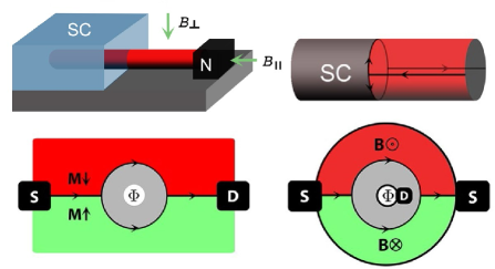
a)

b)

c)

d)

Figure 1: a) An NS junction formed with a TI nanowire. b) Schematic representation of the modes involved in transport: a chiral mode splits into two Majorana modes at the interface, recombines, and exits as a chiral mode again. c) The Majorana interferometer proposed in Refs. Fu and Kane, 2009; Akhmerov et al., 2009. S and D denote source and drain respectively. d) An unfolded representation of the setup in b).

A prominent example of a 1D topological superconductor is realized in semiconducting quantum wires in the presence of a magnetic field Oreg et al. (2010); Lutchyn et al. (2010). Recent transport experiments with such wires aimed to demonstrate the existence of this phase have reported a finite zero-bias conductance across a NS junction Mourik et al. (2012); Das et al. (2012), but the predicted quantization has so far remained a challenge to observe. A possible reason is that these wires typically host several modes Lutchyn et al. (2011); Pientka et al. (2012); Liu et al. (2012); Pikulin et al. (2012); Prada et al. (2012); Rainis et al. (2013) and fine tuning the chemical potential to the single mode regime can be difficult. In the presence of several modes, either a tunnel barrier Mourik et al. (2012); Das et al. (2012) or a quantum point contact Wimmer et al. (2011) may be used to isolate the resonant contribution, but the temperature required to resolve a zero-bias peak then becomes challengingly small. The optimal NS junction to probe this effect should therefore have a robust, easy to manipulate single-mode normal part smoothly interfaced with a superconductor that can be controllably driven into the topological phase.

In this work, we propose to realize such a junction starting from an alternative route to 1D topological superconductivity, recently proposed by Cook and Franz Cook and Franz (2011), based on the use of nanowires made from three dimensional topological insulators (TI). In the nanowire geometry, the 2D surface states of a TI are resolved into a discrete set of modes, with the property that when a parallel flux of $h/2e$ threads the wire, the number of modes is always odd Zhang and Vishwanath (2010); Bardarson et al. (2010); Bardarson and Moore (2013). When a superconducting gap is induced on the surface via the proximity effect, this guarantees that the system becomes a topological superconductor Kitaev (2001); Cook and Franz (2011). An NS junction can then be built be proximitizing only part of the wire, where the superconducting part can be tuned in and out of the topological phase with the in-plane flux Cook and Franz (2011); Ilan et al. (2014).

In addition, our design simultaneously allows to drive the normal region into the single-mode regime by exploiting the unique orbital response of TI surface states to magnetic fields Lee (2009); Vafek (2011); Zhang et al. (2012); Sitte et al. (2012); Brey and Fertig (2014). When a perpendicular field is applied to the normal part of the wire, its top and bottom regions become insulating because of the Quantum Hall Effect. In between these regions, counter-propagating chiral edge states are formed, which are protected from backscattering due to their spatial separation. The resulting NS junction, shown in Fig. 1, has a single chiral mode reflecting from the superconductor, and is ideal for probing conductance quantization. Moreover, all of its components are readily available, as both surface transport in TI nanowires Peng et al. (2009); Xiu et al. (2011); Hong et al. (2014); Dufouleur et al. (2013) and the contacting of bulk TI with superconductors Veldhorst et al. (2012); Williams et al. (2012); Cho et al. (2013) have already been demonstrated experimentally. In the remainder of this paper, we provide a detailed study of the transport properties of this system, demonstrating that conductance quantization is achievable under realistic conditions, and discuss the advantages of our setup over other proposals.

To model the proposed device, we consider a rectangular TI nanowire of height $h$ and width $w$ (perimeter $P=2h+2w$). The surface of the wire is parametrized with two coordinates $(x,s)$, where $s$ is periodic $s\in[0,2\pi]$ and goes around the perimeter of the wire, while $x$ goes along its length. We first consider a magnetic field parallel to the wire, $\vec{B}=(B_{\parallel},0,0)$, described with the gauge choice $\vec{A}=B_{\parallel}(0,-z/2,y/2)$. The dimensionless flux through the wire is $\eta=B_{\parallel}hw/(h/e)$. The effective theory for the surface states is the same as for a cylindrical wire Bardarson et al. (2010); Zhang and Vishwanath (2010), with $s$ the azimuthal angle

$$H_{0}=-iv_{F}\left[\sigma_{x}\partial_{x}+\sigma_{y}(2\pi/P)(\partial_{s}+i\eta)\right],$$ (1)

where we set $\hbar=1$ and take $v_{F}=330$ $\rm meV\,nm$ Liu et al. (2010). The wavefunctions satisfy antiperiodic boundary conditions in $s$ due to the curvature-induced $\pi$ Berry phase Zhang and Vishwanath (2010); Bardarson et al. (2010). The eigenfunctions of $H_{0}$ thus have the form

$$\psi_{k,n}(x,s)=e^{ikx}e^{il_{n}s}\chi_{k,n},$$ (2)

with half-integer angular momentum $l_{n}=n-1/2$ where $n\in\mathbb{Z}$. The spectrum is $E_{k,n}=v_{F}\sqrt{k^{2}+(2\pi/P)^{2}(l_{n}+\eta)^{2}},$ and is depicted in Fig. 2(a). For $\eta=0$ all modes are doubly degenerate, while for $\eta=1/2$ the number of modes is always odd because the $n=0$ one is not degenerate.

By bringing the wire into contact with an $s$-wave superconductor Cook and Franz (2011), as shown in Fig. 1, an $s$-wave pairing potential $\Delta$ is induced due to the proximity effect. The Bogoliubov-de Gennes Hamiltonian can be written as $H=\frac{1}{2}\Psi^{\dagger}\mathcal{H}\Psi$ with

$$\mathcal{H}=\left(\begin{array}[]{cc}H_{0}&\Delta(s)\\ \Delta^{*}(s)&-T^{-1}H_{0}T\end{array}\right),$$ (3)

where $\Psi=(\psi_{\uparrow},\psi_{\downarrow},\psi^{\dagger}_{\downarrow},-\psi^{\dagger}_{\uparrow})$ is a Nambu spinor. The induced pairing potential is $\Delta(s)=\Delta_{0}e^{-in_{v}s}$, where the phase of $\Delta$ can wind around the perimeter with vorticity $n_{v}$. For $\eta=0$ the ground state has $n_{v}=0$. Around $\eta=1/2$, however, it should be energetically favorable for $\Delta$ to develop a vortex . In an actual experiment, $n_{v}$ is expected to jump abruptly as $\eta$ is ramped continuously from zero to $1/2$ Cook et al. (2012). For $\eta$ around 1/2 and in the presence of a vortex, the nanowire becomes a topological superconductor for any $\mu$ within the bulk gap Cook and Franz (2011).

The presence of the vortex is essential in order to observe perfect Andreev reflection in our setup. To see this, consider the Hamiltonian in Eq. (3) in the presence of a NS interface at $x=0$ with $n_{v}$ vortices. Introducing Pauli matrices $\tau_{i}$ acting in Nambu space

$$\mathcal{H}^{(n_{v})}= \left[-i\sigma_{x}\partial_{x}+\sigma_{y}(-i\partial_{s}+\eta\;\tau_{z})2\pi/P-\mu\right]\tau_{z}$$

$$+\Delta_{0}\theta(-x)e^{-i\tau_{z}n_{v}s}\tau_{x}.$$ (4)

For $n_{v}=0$, electron states in the normal part have finite angular momentum $l_{n}$, see Eq. (2), while hole states have angular momentum $-l_{n}$, independently of the value of $\eta$. Since angular momentum must be conserved upon reflection, a single incoming electron can never be reflected as a hole. For $n_{v}=1$ rotational invariance appears to be broken by the pairing term, but is explicitly recovered after the gauge transformation $\Psi\rightarrow e^{i\tau_{z}s/2}\Psi$, which shifts $\eta\rightarrow\eta-1/2$. This transformation also changes the boundary conditions to periodic, such that angular momenta take integer values $l^{\prime}_{n}=n$. As a result, the $n=0$ electron state now has the same angular momentum as its conjugate hole state and can be reflected into it.

The NS conductance of the junction is computed from the Andreev reflection matrix, evaluated separately for every $n$, in a very similar way to Ref. Beenakker, 2006. To compute it, we define incoming $\psi^{e-}_{n}$ and outgoing $\psi^{e+}_{n}$ propagating electron states in the normal part, and similarly for hole states $\psi^{h-}_{n}$ and $\psi^{h+}_{n}$. Normalization is chosen such that all propagating states carry the same current, $J_{x}=\left<\psi|\sigma_{x}|\psi\right>=1$. These are matched to the evanescent states in the superconductor $\psi^{S+}_{n}$ and $\psi^{S-}_{n}$ by imposing continuity of the wavefunction at the junction (dropping the label $n$ for ease of notation)

$$\psi^{e-}+r_{ee}\psi^{e+}+r_{he}\psi^{h-} =a\psi^{S+}+b\psi^{S-},$$ (5)

$$\psi^{h-}+r_{hh}\psi^{h+}+r_{eh}\psi^{e-} =a^{\prime}\psi^{S+}+b^{\prime}\psi^{S-}.$$ (6)

The reflection matrix is defined as $r=\left(\begin{smallmatrix}r_{ee}&r_{eh}\\ r_{he}&r_{hh}\end{smallmatrix}\right),$ and is both unitary and particle-hole symmetric. The conductance is given by $G_{\rm NS}=\frac{2e^{2}}{h}\text{tr}\;r_{eh}r_{eh}^{\dagger},$ where the trace sums over all propagating modes. The resulting $G_{\rm NS}$ for $\Delta_{0}=$ 0.25 meV are shown in Fig. 2(b). When $\eta=1/2$, $n_{v}=1$ and in the range $\mu<\pi/P$, a single mode is reflected from a topological superconductor resulting in a conductance of $2e^{2}/h$.

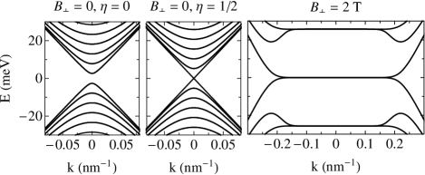
a)

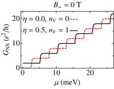
b)

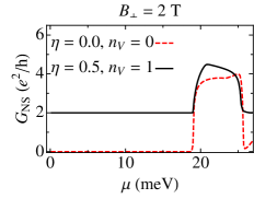
c)

Figure 2: a) The spectrum of a wire of dimensions $h=40$ nm and $w=160$ nm for $B_{\perp}=0$ and $\eta=0$ (left), $B_{\perp}=0$ and $\eta=1/2$ (center) and $B_{\perp}=2T$ (right). Note that in the last case the spectrum is independent of $\eta$. b) NS conductance for $B_{\perp}=0$ and $\Delta_{0}=$ 0.25 meV as a function of $\mu$, for $\eta=0$, $n_{v}=0$ (dashed line) and $\eta=1/2$, $n_{v}=1$ (full line) c) The same for $B_{\perp}=2T$.

The conditions to observe conductance quantization in this setup are not optimal yet, mainly because the chemical potential has to be tuned into a small gap $\pi/P$. This limitation can be overcome by the addition of a perpendicular field. Consider the Hamiltonian of the normal wire with $\vec{B}=(B_{\parallel},B_{\perp},0)$ and a vector potential $\vec{A}=B_{\perp}(z,0,0)+B_{\parallel}(0,-z/2,y/2)$ such that translational invariance is still preserved in the $x$ direction

$$H=\sigma_{x}[-i\partial_{x}+eA_{x}(s)]+\frac{2\pi}{P}\sigma_{y}(-i\partial_{s}+\eta).$$ (7)

The vector potential in the surface coordinates is

$$A_{x}(s)=B_{\perp}P\left\{\begin{array}[]{clcl}-\frac{r}{4}&&\frac{-1+r}{4}&<\frac{s}{2\pi}<\frac{1-r}{4}\\ \frac{s}{2\pi}-\frac{1}{4}&&\frac{1-r}{4}&<\frac{s}{2\pi}<\frac{1+r}{4}\\ \frac{r}{4}&&\frac{1+r}{4}&<\frac{s}{2\pi}<\frac{3-r}{4}\\ -\frac{s}{2\pi}+\frac{3}{4}&&\frac{3-r}{4}&<\frac{s}{2\pi}<\frac{3+r}{4}\end{array}\right.,$$ (12)

with $r=\frac{w}{w+h}$. The profiles of $A_{x}$ and $B_{\perp}$ along the $s$ direction are shown in the inset of Fig. 3(b). Since rotational symmetry is broken, the different $n$ modes are mixed. In the angular momentum basis, Eq. (2), the Hamiltonian is $H=\sum_{n,n^{\prime}=-N}^{N}\chi_{k,n}^{\dagger}H_{n,n^{\prime}}(k)\chi_{k,n^{\prime}},$ where $N$ is an angular momentum cutoff. The matrix element is given by

$$H_{nn^{\prime}}(k) =\left[\sigma_{x}k+\sigma_{y}(2\pi/P)(n-1/2+\eta)\right]\delta_{n,n^{\prime}}$$

$$+\sigma_{x}\sum_{m=-M}^{M}eA^{(m)}_{x}\delta_{n,n^{\prime}+m},$$ (13)

where $A^{(m)}_{x}=\int_{0}^{2\pi}\frac{ds}{2\pi}e^{-ims}A_{x}(s)=B_{\perp}P(-1)^{\frac{m+1}{2}}\sin(m\pi r/2)/m^{2}\pi^{2}$ if $m$ is odd and vanishes otherwise, and $M$ is a cutoff for the number of Fourier components of $A_{x}$, with $M\leq N$. The spectrum of the wire only changes qualitatively when $l_{B}<w$, with $l_{B}=(\hbar/eB_{\perp})^{1/2}$ the magnetic length, and Landau levels start to form in the top and bottom surfaces, which merge smoothly with dispersing chiral states localized in the sides. The spectrum in this regime, shown in Fig. 2(a), becomes independent of $B_{\parallel}$.

The NS conductance for finite $B_{\perp}$ can be computed as before with one important difference: in the basis states for the normal part, the evanescent states (with Im$[k_{ev}]>0$) must be included to obtain a well-defined matching condition. The incoming electron states, labelled now by $\alpha=1,\ldots,N_{\rm prop}$, are $\psi^{e-}_{\alpha}=e^{-ikx}\sum_{n=-N}^{N}e^{il_{n}s}\chi^{e-}_{n,k},$ and similarly for $\psi^{e+}_{\alpha}$, $\psi^{h-}_{\alpha}$ and $\psi^{h+}_{\alpha}$. The evanescent states are defined as $\psi^{N}_{\alpha^{\prime}}$, with $\alpha^{\prime}=1,\ldots,N_{\rm ev}$, with $N_{\rm ev}+N_{\rm prop}=2N$. Both propagating and evanescent momenta and wavefunctions are obtained from the transfer matrix of the normal part Lee and Joannopoulos (1981); Umerski (1997); de Juan et al. . We assume that $B_{\perp}$ is completely screened in the superconducting part of the wire (see Fig. 1), so that the eigenstates in this region remain unchanged. Continuity of the wavefunctions at the interface

$$\psi^{e-}_{\alpha}+\sum_{\beta=1}^{N_{\rm prop}}\left[(r_{ee})_{\alpha\beta}\psi^{e+}_{\beta}+(r_{he})_{\alpha\beta}\psi^{h-}_{\beta}\right]+$$ (14)

$$\sum_{\alpha^{\prime}=1}^{N_{\rm ev}} \left[c_{\alpha\alpha^{\prime}}\psi^{N,e}_{\alpha^{\prime}}+d_{\alpha\alpha^{\prime}}\psi^{N,h}_{\alpha^{\prime}}\right]=\sum_{n=-N}^{N}\left[a_{\alpha n}\psi^{S+}_{n}+b_{\alpha n}\psi^{S-}_{n}\right].$$

For every value of $\alpha$, we project into angular momentum states with $n=-N,\ldots,N$. and since the spinors have four components (spin and particle-hole degrees of freedom) this yields a system of $8N$ equations with $2N_{\rm prop}+2N_{\rm ev}+4N=8N$ coefficients. The system is solved numerically, and the conductance obtained is shown in Fig. 2(c). In the single-mode regime, at zero flux and $n_{v}=0$ we have $G_{\rm NS}=0$, but at $\eta=1/2$ and $n_{v}=1$ (when the superconductor is topological), we have $G_{\rm NS}=2e^{2}/h$ as expected.

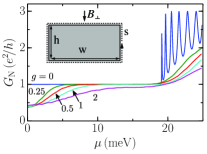
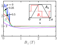
Figure 3: Disorder averaged conductance for a finite wire of dimensions $L=400$ nm, $h=40$ nm and $w=160$ nm for different values of the disorder strength $g$. a) Conductance as a function of chemical potential with fixed magnetic field $B_{\perp}=2$ T. Inset: Cross section of the rectangular wire, with the coordinate $s$ depicted as a dashed arrow. b) Conductance as a function of $B_{\perp}$ at fixed chemical potential $\mu=10$ meV. Inset: The vector potential $A_{x}$ as given by Eq. (12), and its associated magnetic field profile.

The quantization of $G_{\rm NS}$ can be understood intuitively in terms of a 1D low-energy model, depicted in Fig. 1(b), similar to the one describing the Majorana interferometer proposed in Refs. Fu and Kane, 2009; Akhmerov et al., 2009 (see also related studies of Majorana interferometry with chiral Majorana modes Nilsson and Akhmerov (2010); Sau et al. (2011); Li et al. (2012) and Majorana bound states Benjamin and Pachos (2010); Fu (2010); Hassler et al. (2010); Mesaros et al. (2011); Bose and Sodano (2011); Liu and Trauzettel (2011); Strübi et al. (2011); Jacquod and Büttiker (2013); Yamakage and Sato (2014); Ueda and Yokoyama (2014)). In this model, an incoming chiral mode leaving the source is split into two Majorana modes that appear at the interface between the the superconductor and the regions with finite $B_{\perp}$ Tiwari et al. (2013). In the absence of a vortex the two Majoranas recombine as an electron on the other side of the wire and return to the source through the channel of opposite chirality, yielding $G_{\rm NS}=0$. However, if a vortex is present, the two Majoranas accumulate a relative phase of $\pi$ and recombine as a hole, while a Cooper pair is transferred to the superconductor, yielding $G_{\rm NS}=2e^{2}/h$.

The quantization of the conductance in our setup is expected to be robust to disorder to some extent, because transport in the normal part is mediated by spatially separated chiral modes. In order to test this robustness we introduce disorder into the Hamiltonian of a normal wire in the presence of $B_{\perp}$, and compute the two terminal conductance $G_{\rm N}$ of a finite size wire numerically, following the method of Ref. Bardarson et al., 2007. The disorder potential has a correlator $\langle V(r)V(r^{\prime})\rangle=g\frac{(\hbar v_{F})^{2}}{2\pi\xi_{\text{D}}^{2}}e^{-|r-r^{\prime}|^{2}/2\xi_{\text{D}}^{2}},$ with $\xi_{\text{D}}$ the disorder correlation length and $g$ a dimensionless measure of the disorder strength. Our data is obtained by averaging over $10^{3}$ disorder configurations. The results are shown in Fig. 3. In the single-mode regime, the conductance of the normal wire indeed remains quantized to $e^{2}/h$ in the presence of moderate disorder, as long as the chemical potential is not very close to zero. The conductance for each disorder realization is also quantized. A full characterization of the effects of disorder will be presented in a future work de Juan et al. .

Discussion - An important feature of our proposal is that all effects induced by the magnetic field are of purely orbital origin. The Zeeman coupling will be a small correction at the fields considered, and does not change our predictions qualitatively de Juan et al. . In our setup, a quantized conductance can be obtained with both $B_{\perp}=0$ and finite $B_{\perp}$, but the latter case has several advantages that are worth stressing. First, the single-mode regime remains accessible for chemical potentials ranging up to values of the order of the cyclotron frequency $\omega_{c}$, rather than the finite size gap $\pi/P$. Second, chiral mode transport in the normal part is robust against finite disorder due to spatial separation of counter-propagating chiral modes. Third, the spectrum of the normal part in the presence of $B_{\perp}$ becomes independent of $B_{\parallel}$, which affects only the superconducting part. $B_{\parallel}$ thus becomes an independent knob driving the transition from a trivial to a topological superconductor, while the chiral modes remain intact. In this case, measuring $G_{\rm NS}=0$ would represent a genuine consequence of reflection from a trivial superconductor, as opposed to the $B_{\perp}=0$ case where this value of $G_{\rm NS}$ could result from an insulating normal part, see Fig. 2(b).

Our proposal realizes a version of the Majorana interferometer with some important differences. In our setup, instead of contacting the two chiral modes separately the source electrode contacts both channels and the superconductor is the drain Alicea (2012), see Figs. 1(c-d). In addition, the original proposals use ferromagnets and a finite superconducting island to create the Majorana modes, while our setup uses a bulk superconductor and a homogeneous magnetic field Tiwari et al. (2013), making it experimentally more feasible. Despite these differences, the finite voltage and finite temperature behavior of $G_{\rm NS}$will be similar to those in Refs. Fu and Kane, 2009; Akhmerov et al., 2009. This introduces an important advantage to our setup over current semiconducting wires, where the temperatures required to observe conductance quantization are of the order of mK. In our setup, the limiting temperature is determined by the proximity induced gap Akhmerov et al. (2009). Assuming $\Delta_{0}\approx 0.1-0.25$ meV Mourik et al. (2012); Das et al. (2012); Deng et al. (2012) this corresponds to 1-3 K.

Finally, we note that screening $B_{\perp}$ in the SC region requires the use of a superconductor with a high critical field. For example, the superconductor could be a Ti/Nb/Ti trilayer as the one used in the experiment in Ref. Deng et al., 2012, which was estimated to have $H_{c1}=\rm 2.5T$.

We thank J. Dahlhaus, J.E. Moore, A. Vishwanath and J. Analytis for useful discussions. We acknowledge financial support from the “Programa Nacional de Movilidad de Recursos Humanos” (Spanish MECD) (F. de J.) and DARPA FENA (R.I and J.H.B.). R. I. is an Awardee of the Weizmann Institute of Science National Postdoctoral Award Program for Advancing Women in Science.

References

- Nayak et al. (2008) C. Nayak, S. H. Simon, A. Stern, M. Freedman, and S. Das Sarma, Rev. Mod. Phys. 80, 1083 (2008).
- Fu and Kane (2008) L. Fu and C. L. Kane, Phys. Rev. Lett. 100, 096407 (2008).
- Alicea (2012) J. Alicea, Rep. Prog. Phys. 75, 076501 (2012).
- Beenakker (2013) C. Beenakker, Annu. Rev. Con. Mat. Phys. 4, 113 (2013).
- Kitaev (2001) A. Y. Kitaev, Physics-Uspekhi 44, 131 (2001).
- Law et al. (2009) K. T. Law, P. A. Lee, and T. K. Ng, Phys. Rev. Lett. 103, 237001 (2009).
- Fulga et al. (2011) I. C. Fulga, F. Hassler, A. R. Akhmerov, and C. W. J. Beenakker, Phys. Rev. B 83, 155429 (2011).
- Wimmer et al. (2011) M. Wimmer, A. R. Akhmerov, J. P. Dahlhaus, and C. W. J. Beenakker, New J. Phys. 13, 053016 (2011).
- Fu and Kane (2009) L. Fu and C. L. Kane, Phys. Rev. Lett. 102, 216403 (2009).
- Akhmerov et al. (2009) A. R. Akhmerov, J. Nilsson, and C. W. J. Beenakker, Phys. Rev. Lett. 102, 216404 (2009).
- Oreg et al. (2010) Y. Oreg, G. Refael, and F. von Oppen, Phys. Rev. Lett. 105, 177002 (2010).
- Lutchyn et al. (2010) R. M. Lutchyn, J. D. Sau, and S. Das Sarma, Phys. Rev. Lett. 105, 077001 (2010).
- Mourik et al. (2012) V. Mourik, K. Zuo, S. Frolov, S. Plissard, E. Bakkers, and L. Kouwenhoven, Science 336, 1003 (2012).
- Das et al. (2012) A. Das, Y. Ronen, Y. Most, Y. Oreg, M. Heiblum, and H. Shtrikman, Nature Phys. 8, 887 (2012).
- Lutchyn et al. (2011) R. M. Lutchyn, T. D. Stanescu, and S. Das Sarma, Phys. Rev. Lett. 106, 127001 (2011).
- Pientka et al. (2012) F. Pientka, G. Kells, A. Romito, P. W. Brouwer, and F. von Oppen, Phys. Rev. Lett. 109, 227006 (2012).
- Liu et al. (2012) J. Liu, A. C. Potter, K. T. Law, and P. A. Lee, Phys. Rev. Lett. 109, 267002 (2012).
- Pikulin et al. (2012) D. Pikulin, J. Dahlhaus, M. Wimmer, H. Schomerus, and C. Beenakker, New J. Phys. 14, 125011 (2012).
- Prada et al. (2012) E. Prada, P. San-Jose, and R. Aguado, Phys. Rev. B 86, 180503 (2012).
- Rainis et al. (2013) D. Rainis, L. Trifunovic, J. Klinovaja, and D. Loss, Phys. Rev. B 87, 024515 (2013).
- Cook and Franz (2011) A. Cook and M. Franz, Phys. Rev. B 84, 201105 (2011).
- Zhang and Vishwanath (2010) Y. Zhang and A. Vishwanath, Phys. Rev. Lett. 105, 206601 (2010).
- Bardarson et al. (2010) J. H. Bardarson, P. W. Brouwer, and J. E. Moore, Phys. Rev. Lett. 105, 156803 (2010).
- Bardarson and Moore (2013) J. H. Bardarson and J. E. Moore, Rep. Prog. Phys. 76, 056501 (2013).
- Ilan et al. (2014) R. Ilan, J. H. Bardarson, H.-S. Sim, and J. E. Moore, New J. Phys. 16, 053007 (2014).
- Lee (2009) D.-H. Lee, Phys. Rev. Lett. 103, 196804 (2009).
- Vafek (2011) O. Vafek, Phys. Rev. B 84, 245417 (2011).
- Zhang et al. (2012) Y.-Y. Zhang, X.-R. Wang, and X. Xie, J. Phys.: Condens. Matter 24, 015004 (2012).
- Sitte et al. (2012) M. Sitte, A. Rosch, E. Altman, and L. Fritz, Phys. Rev. Lett. 108, 126807 (2012).
- Brey and Fertig (2014) L. Brey and H. A. Fertig, Phys. Rev. B 89, 085305 (2014).
- Peng et al. (2009) H. Peng, K. Lai, D. Kong, S. Meister, Y. Chen, X.-L. Qi, S.-C. Zhang, Z.-X. Shen, and Y. Cui, Nat. Mater. 9, 225 (2009).
- Xiu et al. (2011) F. Xiu, L. He, Y. Wang, L. Cheng, L.-T. Chang, M. Lang, G. Huang, X. Kou, Y. Zhou, X. Jiang, et al., Nat Nanotechnol. 6, 216 (2011).
- Hong et al. (2014) S. S. Hong, Y. Zhang, J. J. Cha, X.-L. Qi, and Y. Cui, Nano Lett. 14, 2815 (2014).
- Dufouleur et al. (2013) J. Dufouleur, L. Veyrat, A. Teichgräber, S. Neuhaus, C. Nowka, S. Hampel, J. Cayssol, J. Schumann, B. Eichler, O. G. Schmidt, B. Büchner, and R. Giraud, Phys. Rev. Lett. 110, 186806 (2013).
- Veldhorst et al. (2012) M. Veldhorst, M. Snelder, M. Hoek, T. Gang, V. Guduru, X. Wang, U. Zeitler, W. van der Wiel, A. Golubov, H. Hilgenkamp, et al., Nat. Mater. 11, 417 (2012).
- Williams et al. (2012) J. Williams, A. Bestwick, P. Gallagher, S. S. Hong, Y. Cui, A. S. Bleich, J. Analytis, I. Fisher, and D. Goldhaber-Gordon, Phys. Rev. Lett. 109, 056803 (2012).
- Cho et al. (2013) S. Cho, B. Dellabetta, A. Yang, J. Schneeloch, Z. Xu, T. Valla, G. Gu, M. J. Gilbert, and N. Mason, Nat. Commun. 4, 1689 (2013).
- Liu et al. (2010) C.-X. Liu, X.-L. Qi, H. Zhang, X. Dai, Z. Fang, and S.-C. Zhang, Phys. Rev. B 82, 045122 (2010).
- Note (1) This is expected to be stable as the flux is repelled by the bulk superconductor and can only be trapped in the region occupied by the wire.
- Cook et al. (2012) A. M. Cook, M. M. Vazifeh, and M. Franz, Phys. Rev. B 86, 155431 (2012).
- Beenakker (2006) C. W. J. Beenakker, Phys. Rev. Lett. 97, 067007 (2006).
- Lee and Joannopoulos (1981) D. H. Lee and J. D. Joannopoulos, Phys. Rev. B 23, 4988 (1981).
- Umerski (1997) A. Umerski, Phys. Rev. B 55, 5266 (1997).
- (44) F. de Juan, J. H. Bardarson, and R. Ilan, in preparation .
- Nilsson and Akhmerov (2010) J. Nilsson and A. R. Akhmerov, Phys. Rev. B 81, 205110 (2010).
- Sau et al. (2011) J. D. Sau, S. Tewari, and S. D. Sarma, Phys. Rev. B 84, 085109 (2011).
- Li et al. (2012) J. Li, G. Fleury, and M. Büttiker, Phys. Rev. B 85, 125440 (2012).
- Benjamin and Pachos (2010) C. Benjamin and J. K. Pachos, Phys. Rev. B 81, 085101 (2010).
- Fu (2010) L. Fu, Phys. Rev. Lett. 104, 056402 (2010).
- Hassler et al. (2010) F. Hassler, A. Akhmerov, C. Hou, and C. Beenakker, New J. Phys. 12, 125002 (2010).
- Mesaros et al. (2011) A. Mesaros, S. Papanikolaou, and J. Zaanen, Phys. Rev. B 84, 041409 (2011).
- Bose and Sodano (2011) S. Bose and P. Sodano, New J. Phys. 13, 085002 (2011).
- Liu and Trauzettel (2011) C.-X. Liu and B. Trauzettel, Phys. Rev. B 83, 220510 (2011).
- Strübi et al. (2011) G. Strübi, W. Belzig, M.-S. Choi, and C. Bruder, Phys. Rev. Lett. 107, 136403 (2011).
- Jacquod and Büttiker (2013) P. Jacquod and M. Büttiker, Phys. Rev. B 88, 241409 (2013).
- Yamakage and Sato (2014) A. Yamakage and M. Sato, Physica E 55, 13 (2014).
- Ueda and Yokoyama (2014) A. Ueda and T. Yokoyama, arXiv:1403.4146 (2014).
- Tiwari et al. (2013) R. P. Tiwari, U. Zülicke, and C. Bruder, Phys. Rev. Lett. 110, 186805 (2013).
- Bardarson et al. (2007) J. H. Bardarson, J. Tworzydło, P. W. Brouwer, and C. W. J. Beenakker, Phys. Rev. Lett. 99, 106801 (2007).
- Deng et al. (2012) M. Deng, C. Yu, G. Huang, M. Larsson, P. Caroff, and H. Xu, Nano Lett. 12, 6414 (2012).