Multiscale Dictionary Learning: Non-Asymptotic Bounds and Robustness

Abstract

High-dimensional datasets are well-approximated by low-dimensional structures. Over the past decade, this empirical observation motivated the investigation of detection, measurement, and modeling techniques to exploit these low-dimensional intrinsic structures, yielding numerous implications for high-dimensional statistics, machine learning, and signal processing. Manifold learning (where the low-dimensional structure is a manifold) and dictionary learning (where the low-dimensional structure is the set of sparse linear combinations of vectors from a finite dictionary) are two prominent theoretical and computational frameworks in this area. Despite their ostensible distinction, the recently-introduced Geometric Multi-Resolution Analysis (GMRA) provides a robust, computationally efficient, multiscale procedure for simultaneously learning manifolds and dictionaries.
   In this work, we prove non-asymptotic probabilistic bounds on the approximation error of GMRA for a rich class of data-generating statistical models that includes “noisy” manifolds, thereby establishing the theoretical robustness of the procedure and confirming empirical observations. In particular, if a dataset aggregates near a low-dimensional manifold, our results show that the approximation error of the GMRA is completely independent of the ambient dimension. Our work therefore establishes GMRA as a provably fast algorithm for dictionary learning with approximation and sparsity guarantees. We include several numerical experiments confirming these theoretical results, and our theoretical framework provides new tools for assessing the behavior of manifold learning and dictionary learning procedures on a large class of interesting models.

Keywords: Dictionary learning, Multi-Resolution Analysis, Manifold Learning, Robustness, Sparsity

1 Introduction

In many high-dimensional data analysis problems, existence of efficient data representations can dramatically boost the statistical performance and the computational efficiency of learning algorithms. Inversely, in the absence of efficient representations, the curse of dimensionality implies that required sample sizes must grow exponentially with the ambient dimension, which ostensibly renders many statistical learning tasks completely untenable. Parametric statistical modeling seeks to resolve this difficulty by restricting the family of candidate distributions for the data to a collection of probability measures indexed by a finite-dimensional parameter. By contrast, nonparametric statistical models are more flexible and oftentimes more precise, but usually require data samples of large sizes unless the data exhibits some simple latent structure (e.g., some form of sparsity). Such structural considerations are essential for establishing convergence rates, and oftentimes these structural considerations are geometric in nature.

One classical geometric assumption asserts that the data, modeled as a set of points in $\mathbb{R}^{D}$, in fact lies on (or perhaps very close to) a single $d$-dimensional affine subspace $V\in\mathbb{R}^{D}$ where $d\ll D$. Tools such as PCA (see Pearson, 1901; Hotelling, 1933, 1936) estimate $V$ in a stable fashion under suitable assumptions. Generalizing this model, one may assert that the data lies on a union of several low-dimensional affine subspaces instead of just one, and in this case the estimation of the multiple affine subspaces from data samples already inspired intensive research due to its subtle complexity (e.g., see Sugaya and Kanatani, 2004; Vidal et al., 2005; Yan and Pollefeys, 2006; Chen and Maggioni, 2011; Ma et al., 2008; Chen and Lerman, 2009; Elhamifar and Vidal, 2009; Zhang et al., 2010; Liu et al., 2010; Ma et al., 2007; Fischler and Bolles, 1981; Tipping and Bishop, 1999; Ho et al., 2003). A widely used form of this model is that of $k$-sparse data, where there exists a dictionary (i.e., a collection of vectors) $\Phi=\{\varphi_{i}\}_{i=1}^{m}\subset\mathbb{R}^{D}$ such that each observed data point $x\in\mathbb{R}^{d}$ may be expressed as a linear combination of at most $k\ll D$ elements of $\Phi$. These sparse representations offer great convenience and expressivity for signal processing tasks (such as in Protter and Elad, 2007; Peyré, 2009), compressive sensing, statistical estimation, and learning (e.g., see Lewicki et al., 1998; Kreutz-Delgado et al., 2003; Maurer and Pontil, 2010; Chen et al., 1998; Donoho, 2006; Aharon et al., 2006; Candes and Tao, 2007, among others), and even exhibits connections with representations in the visual cortex (see Olshausen and Field, 1997). In geometric terminology, such sparse representations are generally attainable when the local intrinsic dimension of the observations is small. For these applications, the dictionary is usually assumed to be known a priori, instead of being learned from the data, but it has been recognized in the past decade that data-dependent dictionaries may perform significantly better than generic dictionaries even in classical signal processing tasks.

The $k$-sparse data model motivates a large amount of research in dictionary learning, where $\Phi$ is learned from data rather than being fixed in advance: given $n$ samples $X_{1},\dots,X_{n}$ from a probability distribution $\mu$ in $\mathbb{R}^{D}$ representing the training data, an algorithm “learns” a dictionary $\widehat{\Phi}$ which provides sparse representations for the observations sampled from $\mu$. This problem and its optimal algorithmic solutions are far from being well-understood, at least compared to the understanding that we have for classical dictionaries such as Fourier, wavelets, curvelets, and shearlets. These dictionaries arise in computational harmonic analysis approaches to image processing, and Donoho (1999) (for example) provides rigorous, optimal approximation results for simple classes of images. The work of Gribonval et al. (2013) present general bounds for the complexity of learning the dictionaries (see also Vainsencher et al., 2011; Maurer and Pontil, 2010, and references therein). The algorithms used in dictionary learning are often computationally demanding, and many of them are based on high-dimensional non-convex optimization (Mairal et al., 2010). The emphasis of existing work is often made on the generality of the approach, where minimal assumptions are made on geometry of the distribution from which the sample is generated. These “pessimistic” techniques incur bounds dependent upon the ambient dimension $D$ in general (even in the standard case of data lying on one hyperplane).

A different type of geometric assumption on the data gives rise to manifold learning, where the observations aggregate on a suitably regular manifold $\mathcal{M}$ of dimension $d$ isometrically embedded in $\mathbb{R}^{D}$ (notable works include Tenenbaum et al., 2000; Roweis and Saul, 2000; Belkin and Niyogi, 2003; Donoho and Grimes, 2002, 2003; Zhang and Zha, 2002; Coifman et al., 2005a, b; Jones et al., 2008, 2010; Coifman and Maggioni, 2006; Genovese et al., 2012b; Little et al., 2009, 2012; Fefferman et al., , among others). This setting has been recognized as useful in a variety of applications (e.g. Coifman et al., 2006; Causevic et al., 2006; Rahman et al., 2005), influencing work in the applied mathematics and machine learning communities during the past several years. It has also been recognized that in many cases the data does not naturally aggregate on a smooth manifold (as in Wakin et al., 2005; Little et al., 2009, 2012), with examples arising in imaging that contradict the smoothness conditions. While this phenomenon is not as widely recognized as it probably could be, we believe that it is crucial to develop methods (both for dictionary and manifold learning) that are robust not only to noise, but also to modeling error. Such concerns motivated the work on intrinsic dimension estimation of noisy data sets (see Little et al., 2009, 2012), where smoothness of the underlying distribution of the data is not assumed, but only certain natural conditions (possibly varying with the scale of the data) are imposed. The central idea of the aforementioned works is to perform the multiscale singular value decomposition (SVD) of the data, an approach inspired by the works of David and Semmes (1993) and Jones (1990) in classical geometric measure theory. These techniques were further extended in several directions in the papers by Chen et al. (2011b, a); Chen and Maggioni (2011), while Chen and Maggioni (2010); Allard et al. (2012) built upon this work to construct multiscale dictionaries for the data based on the idea of Geometric Multi-Resolution Analysis (GMRA).

Until these recent works introduced the GMRA construction, connections between dictionary learning and manifold learning had not garnered much attention in the literature. These papers showed that, for intrinsically low-dimensional data, one may perform dictionary learning very efficiently by exploiting the underlying geometry, thereby illuminating the relationship between manifold learning and dictionary learning. In these papers, it was demonstrated that, in the infinite sample limit and under a manifold model assumption for the distribution of the data (with mild regularity conditions for the manifold), the GMRA algorithm efficiently learns a dictionary in which the data admits sparse representations. More interestingly, the examples in that paper show that the GMRA construction succeeds on real-world data sets which do not admit a structure consistent with the smooth manifold modeling assumption, suggesting that the GMRA construction exhibits robustness to modeling error. This desirable behavior follows naturally from design decisions; GMRA combines two elements that add stability: a multiscale decomposition and localized SVD. Similar ideas appeared in work applying dictionary learning to computer vision problems, for example in the paper by Yu et al. (2009), where local linear approximations are used to create dictionaries. These techniques appeared at roughly the same time as GMRA (Chen and Maggioni (2010)), but were not multiscale in nature, and the selection of the local scale is crucial in applications. These techniques also lacked any finite or infinite sample guarantees, nor considered the effect of noise. They were however successfully applied in computer vision problems, most notably in the Pascal 2007 challenge.

In this paper, we analyze the finite sample behavior of (a slightly modified version of) that construction, and prove strong finite-sample guarantees for its behavior under general conditions on the geometry of a probability distribution generating the data. In particular, we show that these conditions are satisfied when the probability distribution is concentrated “near” a manifold, which robustly accounts for noise and modeling errors. In contrast to the pessimistic bounds mentioned above, the bounds that we prove only depend on the “intrinsic dimension” of the data. It should be noted that our method of proof produces non-asymptotic bounds, and requires several explicit geometric arguments not previously available in the literature (at least to the best of our knowledge). Some of our geometric bounds could be of independent interest to the manifold learning community.

The GMRA construction is therefore proven to simultaneously “learn” manifolds (in sense that it outputs a suitably close approximation to points on a manifold) and dictionaries in which data are represented sparsely. Moreover, the construction is guaranteed to be robust with respect to noise and to the “perturbations” of the manifold model. The GMRA construction is fast, linear in the size of the data matrix, inherently online, does not require nonlinear optimization, and is not iterative. Finally, our results may be combined with recent GMRA compressed sensing techniques and algorithms presented in Iwen and Maggioni (2013), yielding both a method to learn a dictionary in a stable way on a finite set of training data, and a way of performing compressive sensing and reconstruction (with guarantees) from a small number of (suitable) linear projections (again without the need for expensive convex optimization).

This paper is organized as follows: Section 2 introduces the main definitions and notation employed throughout the paper. Section 3 explains the main contributions, formally states the results and provides comparison with existing literature. Finally, Sections 4 and 5 are devoted to the proofs of our main results, Theorem 2 and Theorem 7.

2 Geometric Multi-Resolution Analysis (GMRA)

This section describes the main results of the paper, starting in a somewhat informal form. The statements will be made precise in the course of the exposition. In the statements below, “$\gtrsim$” and “$\lesssim$” denote inequalities up to multiplicative constants and logarithmic factors. Statement of results. Let $\sigma\geq 0$ be a fixed small constant, and let $\varepsilon\gtrsim\sigma$ be given. Suppose that $n\gtrsim\varepsilon^{-(1+d/2)}$, and let $\mathcal{X}_{n}=\{X_{1},\ldots,X_{n}\}$ be an i.i.d. sample from $\Pi$, a probability distribution with density supported in a tube of radius $\sigma$ around a smooth closed $d$-dimensional manifold $\mathcal{M}\hookrightarrow\mathbb{R}^{D}$, with $d>1$. There exists an algorithm that, given $\mathcal{X}_{n}$, outputs the following objects:

• a dictionary $\widehat{\Phi}_{\varepsilon}=\{\widehat{\varphi}_{i}\}_{i\in\mathcal{J}_{\varepsilon}}\subset\mathbb{R}^{D}$;

• a nonlinear “encoding” operator $\widehat{\mathcal{D}}_{\varepsilon}:\mathbb{R}^{D}\rightarrow\mathbb{R}^{\mathcal{J}_{\varepsilon}}$ which takes $x\in\mathbb{R}^{D}$ and returns the coefficients of its approximation by the elements of $\widehat{\Phi}_{\varepsilon}$;

• a “decoding” operator $\widehat{\mathcal{D}}_{\varepsilon}^{-1}:\mathbb{R}^{\mathcal{J}_{\varepsilon}}\rightarrow\mathbb{R}^{D}$ which maps a sequence of coefficients to an element of $\mathbb{R}^{D}$.

Moreover, the following properties hold with high probability:

1. ${\rm Card}(\mathcal{J}_{\varepsilon})\lesssim\varepsilon^{-d/2}$;

2. the image of $\widehat{\mathcal{D}}_{\varepsilon}$ is contained in the set $S_{d+1}\subset\mathbb{R}^{\mathcal{J}_{\varepsilon}}$ of all $(d+1)$ - sparse vectors (i.e., vectors with at most $d+1$ nonzero coordinates);

3. the reconstruction error satisfies

   $$\sup_{x\in{\rm support}(\Pi)}\|x-\widehat{\mathcal{D}}_{\varepsilon}^{-1}\widehat{\mathcal{D}}_{\varepsilon}(x)\| \lesssim\varepsilon;$$

4. the time complexity for computing

   • $\widehat{\Phi}_{\varepsilon}$ is $O(C^{d}(D+d^{2})\varepsilon^{-(1+\frac{d}{2})}\log(1/\varepsilon))$, where $C$ is a universal constant;

   • $\widehat{\mathcal{D}}_{\varepsilon}(x)$ is $O(d(D+d\log(1/\varepsilon)))$, and for $\widehat{\mathcal{D}}_{\varepsilon}^{-1}(x)$ is $O(d(D+\log(1/\varepsilon)))$.

   If a new observation $X_{n+1}$ from $\Pi$ becomes available, $\widehat{\Phi}_{\varepsilon}$ may be updated in time $O(C^{d}(D+d^{2})\log(1/\varepsilon))$.

In other words, we can construct a data-dependent dictionary $\widehat{\Phi}_{\varepsilon}$ of cardinality $O(\varepsilon^{-d/2})$ by looking at $O(\varepsilon^{-1-\frac{d}{2}})$ data points drawn from $\Pi$, such that $\widehat{\Phi}_{\varepsilon}$ provides both $(d+1)$-sparse approximations to data and has expected “reconstruction error” of order $\varepsilon$ (with high probability). Note that the cost of encoding the $(d+1)$ non-zero coefficients requires $O((d+1)\log({\rm Card}(\mathcal{J}_{\varepsilon})))=O(d^{2}\log(1/\epsilon))$. Moreover, the algorithm producing this dictionary is fast and can be quickly updated if new points become available. We want to emphasize that the complexity of our construction only depends on the desired accuracy $\varepsilon$, and is independent of the total number of samples (for example, it is enough to use only the first $\simeq\varepsilon^{-(1+d/2)}$ data points). Many existing techniques in dictionary learning cannot guarantee a requested accuracy, or a given sparsity, and a certain computational cost as a function of the two. Our results above completely characterize the tradeoffs between desired precision, dictionary size, sparsity, and computational complexity for our dictionary learning procedure.

We also remark that a suitable version of compressed sensing applies to the dictionary representations used in the theorem: we refer the reader to the work by Iwen and Maggioni (2013), and its applications to hyperspectral imaging by Chen et al. (2012).

2.1 Notation

For $v\in\mathbb{R}^{D}$, $\|v\|$ denotes the standard Euclidean norm in $\mathbb{R}^{D}$. $B_{d}(0,r)$ is the Euclidean ball in $\mathbb{R}^{d}$ of radius $r$ centered at the origin, and we let $B(0,r):=B_{D}(0,r)$. $\mathop{{\rm Proj}}_{V}$ stands for the orthogonal projection onto a linear subspace $V\subseteq\mathbb{R}^{D}$, $\dim(V)$ for its dimension and $V^{\perp}$ for its orthogonal complement. For $x\in\mathbb{R}^{D}$, let $\mathop{{\rm Proj}}_{x+V}$ be the affine projection onto the affine subspace $x+V$ defined by $\mathop{{\rm Proj}}_{x+V}(y)=x+\mathop{{\rm Proj}}_{V}(y-x)$, for $y\in\mathbb{R}^{D}$.

Given a matrix $A\in\mathbb{R}^{k\times l}$, we write $A=[a_{1}|\cdots|a_{l}]$, where $a_{i}$ stands for the $i$th column of $A$. The operator norm is denoted by $\|A\|$, the Frobenius norm by $\|A\|_{F}$ and the matrix transpose by $A^{T}$. If $k=l$, ${\rm tr\,}(A)$ denotes the trace. For $v\in\mathbb{R}^{k}$, let $\mathop{\rm diag}(v)$ be the $k\times k$ diagonal matrix with $(\mathop{\rm diag}(v))_{ii}=v_{i},\ i=1,\ldots,k$. Finally, we use ${\rm span}\{a_{i}\}_{i=1}^{l}$ to denote the linear span of the columns of $A$.

Given a $C^{2}$ function $f:\mathbb{R}^{l}\rightarrow\mathbb{R}^{k}$, let $f_{i}$ denote the $i$th coordinate of the function $f$ for $i=1,\ldots k$, $Df(v)$ the Jacobian of $f$ at $v\in\mathbb{R}^{l}$, and $D^{2}f_{i}(v)$ the Hessian of the $i$th coordinate at $v$.

We shall use $d{\rm Vol}$ to denote Lebesgue measure on $\mathbb{R}^{D}$, and if $U\subset\mathbb{R}^{D}$ is Lebesgue measurable, ${\rm Vol}(U)$ stands for the Lebesgue measure of $U$. We will use $\mathop{\rm Vol}{}_{\mathcal{M}}$ to denote the volume measure on a $d$-dimensional manifold $\mathcal{M}$ in $\mathbb{R}^{D}$ (note that this coincides with the $d$-dimensional Hausdorff measure for the subset $\mathcal{M}$ of $\mathbb{R}^{D}$), $U_{\mathcal{M}}$ - the uniform distribution over $\mathcal{M}$, and $d_{\mathcal{M}}(x,y)$ to denote the geodesic distance between two points $x,y\in\mathcal{M}$. For a probability measure $\Pi$ on $\mathbb{R}^{D}$, ${\rm supp}(\Pi):=\cap_{C\text{ closed},\Pi(C)=1}C$ stands for its support. Finally, for $x,y\in\mathbb{R}$, $x\vee y:=\max(x,y)$.

2.2 Definition of the geometric multi-resolution analysis (GMRA)

We assume that the data are identically, independently distributed samples from a Borel probability measure $\Pi$ on $\mathbb{R}^{D}$. Let $1\leq d\leq D$ be an integer. A GMRA with respect to the probability measure $\Pi$ consists of a collection of (nonlinear) operators $\{P_{j}:\mathbb{R}^{D}\to\mathbb{R}^{D}\}_{j\geq 0}$. For each “resolution level” $j\geq 0$, $P_{j}$ is uniquely defined by a collection of pairs of subsets and affine projections, $\{(C_{j,k},P_{j,k})\}_{k=1}^{N(j)}$, where the subsets $\{C_{j,k}\}_{k=1}^{N(j)}$ form a measurable partition of $\mathbb{R}^{D}$ (that is, members of $\{C_{j,k}\}_{k=1}^{N(j)}$ are pairwise disjoint and the union of all members is $\mathbb{R}^{D}$). $P_{j}$ is constructed by piecing together local affine projections. Namely, let

$$P_{j,k}(x):=c_{j,k}+\mathop{{\rm Proj}}{}_{V_{j,k}}(x-c_{j,k}),$$

where $c_{j,k}\in\mathbb{R}^{D}$ and $V_{j,k}$ are defined as follows. Let $\mathbb{E}_{j,k}$ stand for the expectation with respect to the conditional distribution $d\Pi_{j,k}(x)=d\Pi(x|x\in C_{j,k})$. Then

$$c_{j,k} =\mathbb{E}_{j,k}x,$$ (1)

$$V_{j,k} =\mathop{\rm argmin~{}}_{\dim(V)=d}\mathbb{E}_{j,k}\left\|x-c_{j,k}-\mathop{{\rm Proj}}{}_{V}(x-c_{j,k})\right\|^{2},$$ (2)

where the minimum is taken over all linear spaces $V$ of dimension $d$. In other words, $c_{j,k}$ is the conditional mean and $V_{j,k}$ is the subspace spanned by eigenvectors corresponding to $d$ largest eigenvalues of the conditional covariance matrix

$$\Sigma_{j,k}=\mathbb{E}_{j,k}[(x-c_{j,k})(x-c_{j,k})^{T}]\,.$$ (3)

Note that we have implicitly assumed that such a subspace $V_{j,k}$ is unique, which will always be the case throughout this paper. Given such a $\{(C_{j,k},P_{j,k})\}_{k=1}^{N(j)}$, we define

$$P_{j}(x):=\sum_{k=1}^{N(j)}I\{x\in C_{j,k}\}P_{j,k}(x)$$

where $I\{x\in C_{j,k}\}$ is the indicator function of the set $C_{j,k}$.

It was shown in the paper by Allard et al. (2012) that if $\Pi$ is supported on a smooth, closed $d$-dimensional submanifold $\mathcal{M}\hookrightarrow\mathbb{R}^{D}$, and if the partitions $\{C_{j,k}\}_{j=1}^{N(j)}$ satisfy some regularity conditions for each $j$, then, for any $x\in\mathcal{M}$, $\|x-P_{j}(x)\|\leq C(\mathcal{M})2^{-2j}$ for all $j\geq j_{0}(\mathcal{M})$. This means that the operators $P_{j}$ provide an efficient “compression scheme” $x\mapsto P_{j}(x)$ for $x\in\mathcal{M}$, in the sense that every $x$ can be well-approximated by a linear combination of at most $d+1$ vectors from the dictionary $\Phi_{2^{-2j}}$ formed by $\{c_{j,k}\}_{k=1}^{N(j)}$ and the union of the bases of $V_{j,k},\ k=1\ldots N(j)$. Furthermore, operators efficiently encoding the “difference” between $P_{j}$ and $P_{j+1}$ were constructed, leading to a multiscale compressible representation of $\mathcal{M}$.

In practice, $\Pi$ is unknown and we only have access to the training data $\mathcal{X}_{n}=\{X_{1},\ldots,X_{n}\}$, which are assumed to be i.i.d. with distribution $\Pi$. In this case, operators $P_{j}$ are replaced by their estimators

$$\widehat{P}_{j}(x):=\sum_{k=1}^{N(j)}I\{x\in C_{j,k}\}\widehat{P}_{j,k}(x)$$

where $\{C_{j,k}\}_{k=1}^{N(j)}$ is a suitable partition of $\mathbb{R}^{D}$ obtained from the data,

$$\widehat{P}_{j,k}(x):=\widehat{c}_{j,k}+\mathop{{\rm Proj}}{}_{\widehat{V}_{j,k}}(x-\widehat{c}_{j,k}),$$ (4)

$$\widehat{c}_{j,k}:=\frac{1}{|\mathcal{X}_{j,k}|}\sum_{x\in\mathcal{X}_{j,k}}x,$$

$$\widehat{V}_{j,k}:=\mathop{\rm argmin~{}}_{\dim(V)=d}\frac{1}{|\mathcal{X}_{j,k}|}\sum_{x\in\mathcal{X}_{j,k}}\left\|x-\widehat{c}_{j,k}-\mathop{{\rm Proj}}{}_{V}(x-\widehat{c}_{j,k})\right\|^{2},$$

$\mathcal{X}_{j,k}=C_{j,k}\cap\mathcal{X}_{n}$, and $|\mathcal{X}_{j,k}|$ denotes the number of elements in $\mathcal{X}_{j,k}$. We shall call these $\widehat{P}_{j}$ the empirical GMRA.

Moreover, the dictionary $\widehat{\Phi}_{2^{-2j}}$ is formed by $\{\hat{c}_{j,k}\}_{k=1}^{N(j)}$ and the union of bases of $\hat{V}_{j,k},\ k=1\ldots N(j)$. The “encoding” and “decoding” operators $\widehat{\mathcal{D}}_{2^{-2j}}$ and $\widehat{\mathcal{D}}_{2^{-2j}}^{-1}$ mentioned above are now defined in the obvious way, so that $\widehat{\mathcal{D}}_{2^{-2j}}^{-1}\widehat{\mathcal{D}}_{2^{-2j}}(x)=\widehat{P}_{j,k}(x)$ for any $x\in C_{j,k}$.

We remark that the “intrinsic dimension” $d$ is assumed to be known throughout this paper. In practice, it can be estimated within the GMRA construction using the “multiscale SVD” ideas of Little et al. (2009, 2012). The estimation technique is based on inspecting (for a given point $x\in C_{j,k}$) the behavior of the singular values of the covariance matrix $\Sigma_{j,k}$ as $j$ varies. For alternative methods, see Levina and Bickel (2004); Camastra and Vinciarelli (2001) and references therein and in the review section of Little et al. (2012).

3 Main results

Our main goal is to obtain probabilistic, non-asymptotic bounds on the performance of the empirical GMRA under certain structural assumptions on the underlying distribution of the data. In practice, the data rarely belongs precisely to a smooth low-dimensional submanifold. One way to relax this condition is to assume that it is “sufficiently close” to a reasonably regular set. Here we assume that the underlying distribution is supported in a thin tube around a manifold. We may interpret the displacement from the manifold as noise, in which case we are making no assumption on distribution of the noise besides boundedness. Another way to model this situation is to allow additive noise, whence the observations are assumed to be of the form $X=Y+\xi$, where $Y$ belongs to a submanifold of $\mathbb{R}^{D}$, $\xi$ is independent of $Y$, and the distribution of $\xi$ is known. This leads to a singular deconvolution problem (see Koltchinskii, 2000; Genovese et al., 2012b). Our assumptions however may also be interpreted as relaxing the “manifold assumption”: even in the absence of noise we do allow data to be not exactly supported on a manifold. Our results will elucidate how the error of sparse approximation via GMRA depends on the “thickness” of the tube, which quantifies stability and robustness properties of our algorithm.

As we mentioned before, our GMRA construction is entirely data-dependent: it takes the point cloud of cardinality $n$ as an input and for every $j\in\mathbb{Z}_{+}$ returns the partition $\{C_{j,k}\}_{k=1}^{N(j)}$ and associated affine projectors $\widehat{P}_{j,k}$. We will measure performance of the empirical GMRA by the $L_{2}(\Pi)$-error

$$\mathbb{E}\left\|X-\widehat{P}_{j}(X)\right\|^{2}:=\int\limits_{{\rm supp}(\Pi)}\left\|x-\widehat{P}_{j}(x)\right\|^{2}d\Pi(x)$$ (5)

or by the $\|\cdot\|_{\infty,\Pi}$-error defined as

$$\left\|\mathop{\rm Id}-\widehat{P}_{j}\right\|_{\infty,\Pi}:=\sup_{x\in{\rm supp}(\Pi)}\left\|x-\widehat{P}_{j}(x)\right\|,$$ (6)

where $\widehat{P}_{j}$ is defined by (4). Note, in particular, that these errors are “out-of-sample”, i.e. measure the accuracy of the GMRA representations on all possible samples, not just those used to train the GMRA, which would not correspond to a learning problem.

The presentation is structured as follows: we start from the natural decomposition

$$\left\|x-\widehat{P}_{j}(x)\right\|\leq\underbrace{\left\|x-P_{j}(x)\right\|}_{\text{approximation error}}+\underbrace{\left\|P_{j}(x)-\widehat{P}_{j}(x)\right\|}_{\text{random error}}$$

and state the general conditions on the underlying distribution and partition scheme that suffice to guarantee that

1. the distribution-dependent operators $P_{j}$ yield good approximation, as measured by $\mathbb{E}\left\|x-P_{j}(x)\right\|^{2}$: this is the bias (squared) term, which is non-random;

2. the empirical version $\widehat{P}_{j}$ is with high probability close to $P_{j}$, so that $\mathbb{E}\left\|\widehat{P}_{j}(x)-P_{j}(x)\right\|^{2}$ is small (with high probability): this is the variance term, which is random.

This leads to our first result, Theorem 2, where the error $\mathbb{E}\left\|x-\widehat{P}_{j}(x)\right\|^{2}$ of the empirical GMRA is bounded with high probability.

We will state this first result in a rather general setting (assumptions A1-A4) below), and after developing this general result, we consider the special but important case where the distribution $\Pi$ generating the data is supported in thin tube around a smooth submanifold, and for a (concrete, efficiently computable, online) partition scheme we show that the conditions of Theorem 2 are satisfied. This is summarized in the statement of Theorem 7, that may be interpreted as proving finite-sample bounds for our GMRA-based dictionary learning scheme for high-dimensional data that suitably concentrates around a manifold. It is important to note that most of the constants in our results are explicit. The only geometric parameters involved in the bounds are the dimension $d$ of the manifold (but not the ambient dimension $D$), its reach (see $\tau$ in (9)) and the “tube thickness” $\sigma$.

Among the existing literature, the papers Allard et al. (2012); Chen et al. (2012) introduced the idea of using multiscale geometric decomposition of data to estimate the distribution of points sampled in high-dimensions. However in the first paper no finite sample analysis was performed, and in the second the connection with geometric properties of the distribution of the data is not made explicit, with the conditions are expressed in terms of certain approximation spaces within the space of probability distributions in $\mathbb{R}^{D}$, with Wasserstein metrics used to measure distances and approximation errors.

The recent paper by Canas et al. (2012) is close in scope to our work; its authors present probabilistic guarantees for approximating a manifold with a global solution of the so-called $k$-flats (Bradley and Mangasarian, 2000) problem in the case of distributions supported on manifolds. It is important to note, however, that our estimator is explicitly and efficiently computable, while exact global solution of $k$-flats is usually unavailable and certain approximations have to be used in practice, with convergence to a global minimum is conditioned on suitable unknown initializations. In practice it is often reported that there exist many local minima with very different values, and good initializations are not trivial to find. In this work we obtain better convergence rates, with fast algorithms, and we also seamlessly tackle the case of noise and model error, which is beyond what was studied previously. We consider this development extremely relevant in applications, both because real data is corrupted by noise and the assumption that data lies exactly on a smooth manifold is often unrealistic. A more detailed comparison of theoretical guarantees for $k$-flats and for our approach is given after we state the main results in Subsection 3.2 below.

Another body of literature connected to this work studies the complexity of dictionary learning. For example, Gribonval et al. (2013) present general bounds for the convergence of global minimums of empirical risks in dictionary learning optimization problems (those results build on and generalize the works of Maurer and Pontil (2010); Vainsencher et al. (2011), among several others). While the rates obtained in those works seem to be competitive with our rates in certain regimes, the fact that their bounds must hold over entire families of dictionaries implies that those error rates generally involve a scaling constant of the order $\sqrt{Dk}$, where $D$ is the ambient dimension and $k$ is the number of “atoms” in the dictionary. Our bounds are independent of the ambient dimension $D$ but implicitly include terms which depend upon the number of our “atoms.” It should be noted that the number of atoms in the dictionary learned by GMRA increase so as to approximate the fine structure of a dataset with more precision. As such, our attainment of the minimax lower bounds for manifold estimation in the Hausdorff metric (obtained in (Genovese et al., 2012a)) should be expected. While dictionaries produced from dictionary learning should reveal the fine structure of a dataset through careful examination of the representations they induce, these representations are often ambiguous unless additional structure is imposed on both the dictionaries and the datasets. On the other hand, the GMRA construction induces completely unambiguous sparse representations that can be used in regression and classification tasks with confidence.

In the course of the proof, we obtain several results that should be of independent interest. In particular, Lemma 18 gives upper and lower bounds for the volume of the tube around a manifold in terms of the reach (7) and tube thickness. While the exact tubular volumes are given by Weyl’s tube formula (see Gray, 2004), our bound are exceedingly easy to state in terms of simple global geometric parameters.

For the details on numerical implementation of GMRA and its modifications, see the works by Allard et al. (2012); Chen and Maggioni (2010).

3.1 Finite sample bounds for empirical GMRA

In this section, we shall present the finite sample bounds for the empirical GMRA described above. For a fixed resolution level $j$, we first state sufficient conditions on the distribution $\Pi$ and the partition $\{C_{j,k}\}_{k=1}^{N(j)}$ for which these $L_{2}(\Pi)$-error bounds hold (see Theorem 2 below).

Suppose that for all integers $j_{\min}\leq j\leq j_{\max}$ the following is true:

(A1)

There exists an integer $1\leq d\leq D$ and a positive constant $\theta_{1}=\theta_{1}(\Pi)$ such that for all $k=1,\ldots,N(j)$,

$$\Pi(C_{j,k})\geq\theta_{1}2^{-jd}\,.$$

(A2)

There is a positive constant $\theta_{2}=\theta_{2}(\Pi)$ such that for all $k=1,\ldots,N(j)$, if $X$ is drawn from $\Pi_{j,k}$ then, $\Pi$ - almost surely,

$$\|X-c_{j,k}\|\leq\theta_{2}2^{-j}\,.$$

(A3)

Let $\lambda^{j,k}_{1}\geq\ldots\geq\lambda^{j,k}_{D}\geq 0$ denote the eigenvalues of the covariance matrix $\Sigma_{j,k}$ (defined in (3)). Then there exist $\sigma=\sigma(\Pi)\geq 0$, $\theta_{3}=\theta_{3}(\Pi)$, $\theta_{4}=\theta_{4}(\Pi)>0$, and some $\alpha>0$ such that for all $k=1\ldots N(j)$,

$$\lambda^{j,k}_{d} \geq\theta_{3}\frac{2^{-2j}}{d}\quad\mbox{ and }\quad\sum\limits_{l=d+1}^{D}\lambda^{j,k}_{l}\leq\theta_{4}(\sigma^{2}+2^{-2(1+\alpha)j})\leq\frac{1}{2}\lambda^{j,k}_{d}.$$

If in addition

(A4)

There exists $\theta_{5}=\theta_{5}(\Pi)$ such that

$$\left\|\mathop{\rm Id}-P_{j}\right\|_{\infty,\Pi}\leq\theta_{5}\left(\sigma+2^{-(1+\alpha)j}\right),$$

then the bounds are also guaranteed to hold for the $\|\cdot\|_{\infty,\Pi}$-error (6).

Remark 1

1. Assumption (A1) entails that the distribution assigns a reasonable amount of probability to each partition element, assumption (A2) ensures that samples from partition elements are always within a ball around the centroid, and assumption (A3) controls the effective dimensionality of the samples within each partition element. Assumption (A4) just assumes a bound on the error for the theoretical GMRA reconstruction.

2. Note that the constants $\theta_{i},\ i=1\ldots 4$, are independent of the resolution level $j$.

3. It is easy to see that Assumption (A3) implies a bound on the “local approximation error”: since $P_{j}$ acts on $C_{j,k}$ as an affine projection on the first $d$ “principal components”, we have

   $$\mathbb{E}_{j,k}\|x-P_{j}(x)\|^{2} ={\rm tr\,}\left[\mathbb{E}_{j,k}\left(x-c_{j,k}-\mathop{{\rm Proj}}{}_{V_{j,k}}(x))(x-c_{j,k}-\mathop{{\rm Proj}}{}_{V_{j,k}}(x)\right)^{T}\right]$$

   $$=\sum\limits_{l=d+1}^{D}\lambda^{j,k}_{l}\leq\theta_{4}(\sigma^{2}+2^{-2(1+\alpha)j}).$$

4. The parameter $\sigma$ is introduced to cover “noisy” models, including the situations when $\Pi$ is supported in a thin tube of width $\sigma$ around a low-dimensional manifold $\mathcal{M}$. Whenever $\Pi$ is supported on a smooth $d$-dimensional manifold, $\sigma$ can be taken to be $0$.

5. The stipulation

   $$\theta_{4}(\sigma^{2}+2^{-2(1+\alpha)j})\leq\frac{1}{2}\lambda^{j,k}_{d}$$

   guarantees that the spectral gap $\lambda^{j,k}_{d}-\lambda^{j,k}_{d+1}$ is sufficiently large.

We are in position to state our main result.

Theorem 2

Suppose that (A1)-(A3) are satisfied, let $X,X_{1},\ldots,X_{n}$ be an i.i.d. sample from $\Pi$, and set $\bar{d}:=4d^{2}\theta_{2}^{4}/\theta_{3}^{2}$. Then for any $j_{\min}\leq j\leq j_{\max}$ and any $t\geq 1$ such that $t+\log(\bar{d}\vee 8)\leq\frac{1}{2}\theta_{1}n2^{-jd}$,

$$\mathbb{E}\|X-\widehat{P}_{j}(X)\|^{2}\leq 2\theta_{4}\left(\sigma^{2}+2^{-2j(1+\alpha)}\right)+c_{1}2^{-2j}\frac{(t+\log(\bar{d}\vee 8))d^{2}}{n2^{-jd}},$$

and if in addition (A4) is satisfied,

$$\left\|\mathop{\rm Id}-\widehat{P}_{j}\right\|_{\infty,\Pi}\leq\theta_{5}\left(\sigma+2^{-(1+\alpha)j}\right)+\sqrt{\frac{c_{1}}{2}2^{-2j}\frac{(t+\log(\bar{d}\vee 8))d^{2}}{n2^{-jd}}}$$

with probability $\geq 1-\frac{2^{jd+1}}{\theta_{1}}\left(e^{-t}+e^{-\frac{\theta_{1}}{16}n2^{-jd}}\right)$, where $c_{1}=2\left(12\sqrt{2}\frac{\theta_{2}^{3}}{\theta_{3}\sqrt{\theta_{1}}}+4\sqrt{2}\frac{\theta_{2}}{d\sqrt{\theta_{1}}}\right)^{2}$.

3.2 Distributions concentrated near smooth manifolds

Of course, the statement of Theorem 2 has little value unless assumptions (A1)-(A4) can be verified for a rich class of underlying distributions. We now introduce an important class of models and an algorithm to construct suitable partitions $\{C_{j,k}\}$ which together satisfy these assumptions. Let $\mathcal{M}$ be a smooth (or at least $C^{2}$, so changes of coordinate charts admit continuous second-order derivatives), closed $d$-dimensional submanifold of $\mathbb{R}^{D}$. We recall the definition of the reach (see Federer, 1959), an important global characteristic of $\mathcal{M}$. Let

$$D(\mathcal{M}) =\{y\in\mathbb{R}^{D}:\exists!x\in\mathcal{M}\text{ s.t. }\|x-y\|=\inf_{z\in\mathcal{M}}\|z-y\|\},$$ (7)

$$\mathcal{M}_{r} =\{y\in\mathbb{R}^{D}:\ \inf_{x\in\mathcal{M}}\|x-y\|<r\}.$$ (8)

Then

$${\rm reach}(\mathcal{M}):=\sup\{r\geq 0:\ \mathcal{M}_{r}\subseteq D(\mathcal{M})\},$$ (9)

and we shall always use $\tau$ to denote the reach of the manifold $\mathcal{M}$.

Definition 3

Assume that $0\leq\sigma<\tau$. We shall say that the distribution $\Pi$ satisfies the $(\boldsymbol{\tau},\boldsymbol{\sigma})$-model assumption if there exists a smooth (or at least $C^{2}$), compact submanifold $\mathcal{M}\hookrightarrow\mathbb{R}^{D}$ with reach $\tau$ such that ${\rm supp}(\Pi)=\mathcal{M}_{\sigma}$, $\Pi$ and $\mathcal{U}_{\mathcal{M}_{\sigma}}$ (the uniform distribution on $\mathcal{M}_{\sigma}$) are absolutely continuous with respect to each other, and so Radon-Nikodym derivative $\frac{d\Pi}{dU_{\mathcal{M}_{\sigma}}}$ satisfies

$$0<\phi_{1}\leq\frac{d\Pi}{d\mathcal{U}_{\mathcal{M}_{\sigma}}}\leq\phi_{2}<\infty\qquad\mathcal{U}_{\mathcal{M}_{\sigma}}\text{- almost surely}\,.$$ (10)

Example 1

Consider the unit sphere of radius $R$ in $\mathbb{R}^{D}$, $\mathcal{S}_{R}$. Then $\tau=R$ for this manifold, and for any $\sigma<R$, the uniform distribution on the set $B(0,R+\sigma)\setminus B(0,R-\sigma)$ satisfies the $(\sigma,\tau)$-model assumption. On the other hand, taking the uniform distribution on a $\sigma$-thickening of the union of two line segments emanating from the origin produces a distribution which does not satisfy the $(\sigma,\tau)$ model assumption. In particular, $\tau=0$ for the underlying manifold.

Remark 4

We will implicitly assume that constants $\phi_{1}$ and $\phi_{2}$ do not depend on the ambient dimension $D$ (or depend on a slowly growing function of $D$, such as $\log D$) - the bound of Theorem 7 shows that this is the “interesting case”. On the other hand, we often do not need the full power of $(\tau,\sigma)$ - model assumption, see the Remark 9 after Theorem 7.

Our partitioning scheme is based on the data structure known as the cover tree introduced by Beygelzimer et al. (2006) (see also Karger and Ruhl, 2002; Yianilos, 1993; Ciaccia et al., 1997). We briefly recall its definition and basic properties. Given a set of $n$ distinct points $S_{n}=\{x_{1},\ldots,x_{n}\}$ in some metric space $(S,\rho)$, the cover tree $T$ on $S_{n}$ satisfies the following: let $T_{j}\subset S_{n},\ j=0,1,2,\ldots$ be the set of nodes of $T$ at level $j$. Then

1. $T_{j}\subset T_{j+1}$;

2. for all $y\in T_{j+1}$, there exists $z\in T_{j}$ such that $\rho(y,z)<2^{-j}$;

3. for all $y,z\in T_{j}$, $\rho(y,z)>2^{-j}$.

Remark 5

Note that these properties imply the following: for any $y\in S_{n}$, there exists $z\in T_{j}$ such that $\rho(y,z)<2^{-j+1}$.

Theorem 3 in (Beygelzimer et al., 2006) shows that the cover tree always exists; for more details, see the aforementioned paper.

We will construct a cover tree for the collection $X_{1},\ldots,X_{n}$ of i.i.d. samples from the distribution $\Pi$ with respect to the Euclidean distance $\rho(x,y):=\|x-y\|$. Assume that $T_{j}:=T_{j}(X_{1},\ldots,X_{n})=\{a_{j,k}\}_{k=1}^{N(j)}$. Define the indexing map

$$k(x):=\mathop{\rm argmin~{}}_{1\leq k\leq N(j)}\|x-a_{j,k}\|$$

(ties are broken by choosing the smallest value of $k$), and partition $\mathbb{R}^{D}$ into the Voronoi regions

$$C_{j,k}=\{x\in\mathbb{R}^{D}:k_{j}(x)=k\}.$$ (11)

Let $\varepsilon(n,t)$ be the smallest $\varepsilon>0$ which satisfies

$$n\geq\frac{1}{\phi_{1}}\left(\frac{\tau+\sigma}{\tau-\sigma}\right)^{d}\beta_{1}\left(\log\beta_{2}+t\right),$$ (12)

where $\beta_{1}=\frac{\mathop{\rm Vol}{}_{\mathcal{M}}(\mathcal{M})}{\cos^{d}(\delta_{1}){\rm Vol}(B_{d}(0,\varepsilon/4))}$, $\beta_{2}=\frac{\mathop{\rm Vol}{}_{\mathcal{M}}(\mathcal{M})}{\cos^{d}(\delta_{2}){\rm Vol}(B_{d}(0,\varepsilon/8))}$, $\delta_{1}=\arcsin(\varepsilon/8\tau)$, and $\delta_{2}=\arcsin(\varepsilon/16\tau)$.

Remark 6

For large enough $n$, this requirement translates into $n\geq C(\mathcal{M},d,\phi_{1})\left(\frac{1}{\varepsilon}\right)^{d}\left(\log\frac{1}{\varepsilon}+t\right)$ for some constant $C(\mathcal{M},d,\phi_{1})$.

We are ready to state the main result of this section.

Theorem 7

Suppose that $\Pi$ satisfies the $(\tau,\sigma)$-model assumption. Let $X_{1},\ldots,X_{n}$ be an i.i.d. sample from $\Pi$, construct a cover tree $T$ from $\{X_{i}\}_{i=1}^{n}$, and define $C_{j,k}$ as in (11). Assume that $\varepsilon(n,t)<\sigma$. Then, for all $j\in\mathbb{Z}_{+}$ such that $2^{-j}>8\sigma$ and $3\cdot 2^{-j}+\sigma<\tau/8$, the partition $\{C_{j,k}\}_{k=1}^{N(j)}$ and $\Pi$ satisfy (A1), (A2), (A3), and (A4) with probability $\geq 1-e^{-t}$ for

$$\theta_{1} =\frac{\phi_{1}{\rm Vol}(B_{d}(0,1))}{2^{4d}\mathop{\rm Vol}{}_{\mathcal{M}}(\mathcal{M})}\left(\frac{\tau-\sigma}{\tau+\sigma}\right)^{d},$$

$$\theta_{2} =12,$$

$$\theta_{3} =\frac{\phi_{1}/\phi_{2}}{2^{4d+8}\left(1+\frac{\sigma}{\tau}\right)^{d}},$$

$$\theta_{4} =2\vee\frac{2^{3}3^{4}}{\tau^{2}},$$

$$\theta_{5} =\left(2\vee\frac{2^{2}3^{2}}{\tau}\right)\left(1+3\cdot 2^{5}\sqrt{2d}\left(1+\frac{\sigma}{\tau}\right)^{d/2}\left(\frac{1+\left(\frac{25}{71}\right)^{2}}{1-\frac{1}{9\cdot 2^{12}}}\right)^{d/4}\right),$$

$$\alpha =1.$$

One may combine the results of Theorem 7 and Theorem 2 as follows: given an i.i.d. sample $X_{1},\ldots,X_{n}$ from $\Pi$, use the first $\lceil\frac{n}{2}\rceil$ points $\{X_{1},\ldots,X_{\lceil\frac{n}{2}\rceil}\}$ to obtain the partition $\{C_{j,k}\}_{k=1}^{N(j)}$, while the remaining $\{X_{\lceil\frac{n}{2}\rceil+1},\ldots,X_{n}\}$ are used to construct the operator $\hat{P}_{j}$ (see (4)). This makes our GMRA construction entirely (cover tree, partitions, affine linear projections) data-dependent. We observe that since our approximations are piecewise linear, they are insensitive to regularity of the manifold beyond first order, so the estimates saturate at $\alpha=1$.

When $\sigma$ is very small or equal to $0$, the bounds resulting from Theorem 2 can be “optimized” over $j$ to get the following statement (we present only the bounds for the $L_{2}(\Pi)$ error, but the results $\|\cdot\|_{\infty,\Pi}$ are similar).

Corollary 8

Assume that conditions of Theorem 7 hold, and that $n$ is sufficiently large. Then for all $A\geq 1$ such that $A\log n\leq c_{4}n$, the following holds:

(a)

if $d\in\{1,2\}$,

$$\inf\limits_{j\in\mathbb{Z}:2^{-j}<\tau/24}\mathbb{E}\|x-\widehat{P}_{j}(x)\|^{2}\leq C_{1}\left(\frac{\log n}{n}\right)^{\frac{2}{d}};$$

(b)

if $d\geq 3$,

$$\inf\limits_{j\in\mathbb{Z}:2^{-j}<\tau/24}\mathbb{E}\|x-\widehat{P}_{j}(x)\|^{2}\leq C_{2}\left(\frac{\log n}{n}\right)^{\frac{4}{d+2}}$$ (13)

with probability $\geq 1-c_{3}n^{-A}$, where $C_{1}$ and $C_{2}$ depend only on $A,\tau,d,\phi_{1}/\phi_{2},\mathop{\rm Vol}{}_{\mathcal{M}}(\mathcal{M})$ and $c_{3},c_{4}$ depend only on $\tau,d,\phi_{1}/\phi_{2},\mathop{\rm Vol}{}_{\mathcal{M}}(\mathcal{M})$.

Proof  In case (a), it is enough to set $t:=(A+1)\log n$, $2^{-j}:=\left(\frac{16t}{\theta_{1}n}\right)^{1/d}$, and apply Theorem 2. For case (b), set $t:=(A+1)\log n$ and $2^{-j}:=\left(\frac{A\log n}{n}\right)^{\frac{1}{d+2}}$.  
Finally, we note that the claims ii. and iii. stated in the beginning of Section 2 easily follow from our general results (it is enough to choose $n$ such that $\varepsilon\simeq n^{-\frac{2}{d+2}}$ and $2^{-j}=\sqrt{\varepsilon}$). Claim i. follows from assumption (A1) and Theorem 7. Computational complexity bounds iv. follow from the associated computational cost estimates for the cover trees algorithm and the randomized singular value decomposition, and are discussed in detail in Sections 3 and 8 of (Allard et al., 2012).

Remark 9

It follows from our proof that it is sufficient to assume a weaker (but somewhat more technical) form of $(\tau,\sigma)$-model condition for the conclusion of Theorem 7 to hold. Namely, let $\tilde{\Pi}$ be the pushforward of $\Pi$ under the projection $\mathop{{\rm Proj}}{}_{\mathcal{M}}:\mathcal{M}_{\sigma}\rightarrow\mathcal{M}$, and assume that there exists $\tilde{\phi}_{1}>0$ such that for any measurable $A\subseteq\mathcal{M}$

$$\tilde{\Pi}(A):=\Pi\left(\mathop{{\rm Proj}}{}_{\mathcal{M}}^{-1}(A)\right)\geq\tilde{\phi}_{1}U_{\mathcal{M}}(A).$$

Moreover, suppose that there exists $\tilde{\phi}_{2}>0$ such that for any $y\in\mathcal{M}$, any set $A\subset\mathcal{M}_{\sigma}$ and any $\tau>r\geq 2\sigma$ such that $B(y,r)\cap\mathcal{M}_{\sigma}\subseteq A\subseteq B(y,12r)$, we have

$$\Pi(A)\leq\tilde{\phi}_{2}\mathcal{U}_{\mathcal{M}_{\sigma}}(A).$$

In some circumstances, checking these two conditions is not hard (e.g., when $\mathcal{M}$ is a sphere, $Y$ is uniformly distributed on $\mathcal{M}$, $\eta$ is spherically symmetric “noise” independent of $Y$ and such that $\|\eta\|\leq\sigma$, and $\Pi$ is the distribution of $Y+\eta$), but $(\tau,\sigma)$ - assumption does not need to hold with constants $\phi_{1}$ and $\phi_{2}$ independent of $D$.

3.3 Connections to the previous work and further remarks

It is useful to compare our rates with results of Theorem 4 in (Canas et al., 2012). In particular, this theorem implies that, given a sample of size $n$ from the Borel probability measure $\Pi$ on the smooth $d$-dimensional manifold $\mathcal{M}$, the $L_{2}(\Pi)$-error of approximation of $\mathcal{M}$ by $k_{n}=C_{1}(\mathcal{M},\Pi)n^{d/(2(d+4))}$ affine subspaces is bounded by $C_{2}(\mathcal{M},\Pi)n^{-2/(d+4)}$. Here, the dependence of $k_{n}$ on $n$ is “optimal” in a sense that it minimizes the upper bound for the risk obtained in (Canas et al., 2012). If we set $\sigma=0$ in our results, then it easily follows from Theorems 7 and 2 that the $L_{2}(\Pi)$-error achieved by our GMRA construction for $2^{j}\simeq n^{\frac{1}{2(d+4)}}$ (so that $N(j)\simeq k_{n}$ to make the results comparable) is of the same order $n^{-\frac{2}{d+4}}$. However, this choice of $j$ is not optimal in this case - in particular, setting $2^{j_{n}}\simeq n^{\frac{1}{d+2}}$, we obtain as in (13) a $L_{2}(\Pi)$-error of order $n^{-\frac{2}{d+2}}$, which is a faster rate. Moreover, we also obtain results in the $\sup$ norm, and not only for mean square error. We should note that technically our results require the stronger condition (10) on the underlying measure $\Pi$, while theoretical guarantees in (Canas et al., 2012) are obtained assuming only the upper bound $\frac{d\Pi}{dU_{\mathcal{M}}}\leq\phi_{2}<\infty$, where $U_{\mathcal{M}}:=\frac{d\mathop{\rm Vol}{}_{\mathcal{M}}}{\mathop{\rm Vol}{}_{\mathcal{M}}(\mathcal{M})}$ is the uniform distribution over $\mathcal{M}$.

The rate (13) is the same (up to log-factors) as the minimax rate obtained for the problem considered in (Genovese et al., 2012a) of estimating a manifold from the samples corrupted with the additive noise that is “normal to the manifold”. Our theorems are stated under more general conditions, however, we only prove robustness-type results and do not address the problem of denoising. At the same time, the estimator proposed in (Genovese et al., 2012a) is (unlike our method) not suitable for applications. The paper (Genovese et al., 2012b) considers (among other problems) the noiseless case of manifold estimation under Hausdorff loss, and obtains the minimax rate of order $n^{-\frac{2}{d}}$. Performed numerical simulation (see Section 6) suggest that our construction also appears to achieve this rate in the noiseless case. However, our main focus is on the case $\sigma>0$.

The work of Fefferman et al. establishes the sampling complexity of testing the hypothesis if an unknown distribution is close to being on a manifold (with known reach, volume, dimension) in the Mean Squared sense, is also related to the work discussed in this section, and to the present one. While our results do imply that if we have enough points, as prescribed by our main theorems, and the MSE does not decay as prescribed, then the data with high probability does not satisfy the geometric assumptions in the corresponding theorem, this is still different from the hypothesis testing problem. There may distributions not satisfying our assumptions, such that GMRA still yields good approximations: in fact we welcome and do not rule out these situations. Fefferman et al. also present an algorithm for constructing an approximation to the manifold; however such an algorithm does not seem easy to implement in practice. The emphasis in this work is on moving to a more general setting than the manifold setting, focusing on multiscale approaches that are robust (locally, because of SVD, as well as across scales), and fast, easily implementable algorithms.

We remark that we analyze the case of one manifold $\mathcal{M}$, and its “perturbation” in the sense of having a measure supported in a tube around $\mathcal{M}$. Our construction however is multiscale and in particular local. Many extensions are immediate, for example to the case of multiple manifolds (possibly of different dimensions) with non-intersecting tubes around them. The case of unbounded noise is also of interest: if the noise has sub-Gaussian tails then very few points are outside a tube of radius dependent on the sub-Gaussian moment, and these “outliers” are easily disregarded as there are few and far away, so they do not affect the construction and the analysis at fine scales. Another situation is when there are many gross outliers, for example points uniformly distributed in high-dimension in, say, a cube containing $\mathcal{M}$. But then the volume of such cube is so large that unless the number of points is huge (at least exponential in the ambient dimension $D$), almost all of these points are in fact far from each other and from $\mathcal{M}$ with very high probability, so that again they do affect the analysis and the algorithms. These are some of the advantages of the multiscale approach, which would otherwise have the potential of corrupting the results (or complicating the analysis of) other global algorithms, such as $k$-flats.

4 Preliminaries

This section contains the remaining definitions and preliminary technical facts that will be used in the proofs of our main results.

Given a point $y$ on the manifold $\mathcal{M}$, let $T_{y}\mathcal{M}$ be the associated tangent space, and let $T_{y}^{\perp}\mathcal{M}$ be the orthogonal complement of $T_{y}\mathcal{M}$ in $\mathbb{R}^{D}$. We define the projection from the tube $\mathcal{M}_{\sigma}$ (see (8)) onto the manifold $\mathop{{\rm Proj}}{}_{\mathcal{M}}:\mathcal{M}_{\sigma}\rightarrow\mathcal{M}$ by

$$\mathop{{\rm Proj}}{}_{\mathcal{M}}(x)=\mathop{\rm argmin~{}}_{y\in\mathcal{M}}\|x-y\|$$

and note that $\sigma<\tau$, together with (7), implies that $\mathop{{\rm Proj}}{}_{\mathcal{M}}$ is well-defined on $\mathcal{M}_{\sigma}$, and

$$\mathop{{\rm Proj}}{}_{\mathcal{M}}(y+\xi)=y$$

whenever $y\in\mathcal{M}$ and $\xi\in T_{y}^{\perp}\mathcal{M}\cap B(0,\sigma)$.

Next, we recall some facts about the volumes of parallelotopes that will prove useful in Section 5. For a matrix $A\in\mathbb{R}^{k\times l}$ with $l\leq k$, we shall abuse our previous notation and let ${\rm Vol}(A)$ also denote the volume of the parallelotope formed by the columns of $A$. Let $A$ and $B$ be $k\times l_{1}$ and $k\times l_{2}$ matrices respectively with $l_{1}+l_{2}\leq k$, and note that

$${\rm Vol}([A\,|\,B])\leq{\rm Vol}(A){\rm Vol}(B)$$

where $([A\,|\,B])$ denotes the concatenation of $A$ and $B$ into a $k\times(l_{1}+l_{2})$ matrix. Moreover, if the columns of $A$ and $B$ are all mutually orthogonal, we clearly have that ${\rm Vol}([A\,|\,B])={\rm Vol}(A){\rm Vol}(B)$. Assuming that $I$ is the $l_{1}\times l_{1}$ identity matrix, we have the bound ${\rm Vol}\begin{pmatrix}A\\ I\end{pmatrix}\geq 1$. The following proposition gives volume bounds for specific types of perturbations that we shall encounter.

Proposition 10

Suppose $Y=[y_{1}|\cdots|y_{d}]$ is symmetric $d$ by $d$ matrix such that $\|Y\|\leq q<1$. Then

$${\rm Vol}\begin{pmatrix}I+Y\\ X\end{pmatrix} \leq (1+q)^{d}\,{\rm Vol}\begin{pmatrix}I\\ X\end{pmatrix}$$

$${\rm Vol}\begin{pmatrix}I+Y&X^{T}\\ X&-I\end{pmatrix} \geq (1-q)^{d}\,{\rm Vol}\begin{pmatrix}I&X^{T}\\ X&-I\end{pmatrix}.$$

This proof (as well as the proofs of our other supporting technical contributions) is given in the Appendix. Finally, let us recall several important geometric consequences involving the reach:

Proposition 11

The following holds:

1. For all $x,y\in\mathcal{M}$ such that $\|x-y\|\leq\tau/2$, we have

   $$d_{\mathcal{M}}(x,y)\leq\tau-\tau\sqrt{1-2\frac{\|x-y\|}{\tau}}\leq 2\|x-y\|.$$

2. Let $\gamma(t):[0,1]\mapsto\mathcal{M}$ be the arclength-parameterized geodesic. Then $\|\gamma^{\prime\prime}(t)\|\leq\frac{1}{\tau}$ for all $t$.

3. Let $\phi$ be the angle between $T_{x}\mathcal{M}$ and $T_{y}\mathcal{M}$, in other words,

   $$\cos(\phi):=\min_{u\in T_{x}\mathcal{M},\|u\|=1}\max_{v\in T_{y}\mathcal{M},\|v\|=1}\left|\left\langle u,v\right\rangle\right|.$$

   If $\|x-y\|\leq\frac{\tau}{2}$, then $\cos(\phi)\geq\sqrt{1-2\frac{\|x-y\|}{\tau}}.$

4. If $x$ is such that $\|x-y\|<\tau/2$, then $x$ is a regular point of $\mathop{{\rm Proj}}{}_{y+T_{y}\mathcal{M}}:\mathcal{B}(y,\tau/2)\cap\mathcal{M}\rightarrow y+T_{y}\mathcal{M}$ (in other words, the Jacobian of $\mathop{{\rm Proj}}{}_{y+T_{y}\mathcal{M}}$ at $x$ is nonsingular).

5. Let $y\in\mathcal{M}$, $r<\tau$ and $A=\mathcal{M}\cap B(y,r)$. Then

   $$B_{d}(y,r\cos(\theta))\subseteq\mathop{{\rm Proj}}{}_{y+T_{y}\mathcal{M}}(A),$$

   where $\theta=\arcsin\left(\frac{r}{2\tau}\right)$.

Proof  Part i. is the statement of Proposition 6.3 and part ii. - of Proposition 6.1 in (Niyogi et al., 2008). Part iii. is demonstrated in Lemma 5.4 of the same paper, and this lemma coincides with iv. Part v. is proven in Lemma 5.3 of (Niyogi et al., 2008).  

5 Proofs of the main results

The rest of the paper is devoted to the proofs of our main results.

5.1 Overview of the proofs

We begin by providing an overview of the main steps of the proofs to aid comprehension. The proof of Theorem 2 begins by invoking the bias-variance decomposition:

$$\|x-\widehat{P}_{j}(x)\|^{2}\leq 2\|x-P_{j}(x)\|^{2}+2\|P_{j}(x)-\widehat{P}_{j}(x)\|^{2}.$$

Remark 1, part iii. and the decomposition

$$\mathbb{E}\|X-P_{j}(X)\|^{2}=\sum_{k=1}^{N(j)}\Pi(C_{j,k})\mathbb{E}_{j,k}\|X-P_{j}(X)\|^{2}$$

gives us the first term in the bound of Theorem 2. Note that this contribution is deterministic.

The next step in the proof is to bound the stochastic error $\mathbb{E}\|P_{j}(x)-\widehat{P}_{j}(x)\|^{2}$ with high probability. We start with the bound

$$\|P_{j}(x)-\widehat{P}_{j}(x)\| =\|c_{j,k}-\widehat{c}_{j,k}+\mathop{{\rm Proj}}{}_{V_{j,k}}(x-c_{j,k})-\mathop{{\rm Proj}}{}_{\widehat{V}_{j,k}}(x-c_{j,k}+c_{j,k}-\widehat{c}_{j,k})\|$$ (14)

$$\leq 2\|c_{j,k}-\widehat{c}_{j,k}\|+\|\mathop{{\rm Proj}}{}_{V_{j,k}}-\mathop{{\rm Proj}}{}_{\widehat{V}_{j,k}}\|\cdot\|x-c_{j,k}\|.$$ (15)

for $x\in C_{j,k}$. We then use concentration of measure results (matrix Bernstein-type inequality) to bound the terms

$$\|c_{j,k}-\widehat{c}_{j,k}\|\text{ and }\left\|\widehat{\Sigma}_{j,k}-\Sigma_{j,k}\right\|$$

with high probability. The latter bound and Assumption (A3) allows us to invoke Theorem 14 to obtain a bound of the form

$$\|\mathop{{\rm Proj}}{}_{V_{j,k}}-\mathop{{\rm Proj}}{}_{\widehat{V}_{j,k}}\|\leq C\left\|\widehat{\Sigma}_{j,k}-\Sigma_{j,k}\right\|.$$

Finally, the term $\|x-c_{j,k}\|$ is controlled by Assumption (A2).

The proof of Theorem 7 is primarily supported by a volume comparison theorem that allows for the cancellation of the “noisy” terms that would imply dependency on $D$. That is, supposing that $\text{Proj}_{\mathcal{M}}:\mathcal{M}_{\sigma}\rightarrow\mathcal{M}$ is the projection from the $\sigma$-tubular neighborhood onto the underlying manifold with reach $\tau$, if $U\subset\mathcal{M}$ is $\mathop{\rm Vol}{}_{\mathcal{M}}$-measurable with $\mathop{\rm Vol}{}_{\mathcal{M}}(U)>0$, we have that

$$\left(1-\frac{\sigma}{\tau}\right)^{d}\leq\frac{{\rm Vol}(\text{Proj}_{\mathcal{M}}^{-1}(U))}{\mathop{\rm Vol}{}_{\mathcal{M}}(U){\rm Vol}(B_{D-d}(0,\sigma))}\leq\left(1+\frac{\sigma}{\tau}\right)^{d}.$$

This is encapsulated in Lemma 18. This allows us to relate probabilities on the tubular neighborhood with probabilities on the manifold itself, which only involve $d$-dimensional volumes.

The first thing that this allows us to do is to ensure that a sufficiently large sample from $\mathcal{U}_{\mathcal{M}_{\sigma}}$, $\{X_{i}\}_{i=1}^{N}$, has that $\{\text{Proj}_{\mathcal{M}}(X_{i})\}_{i=1}^{N}$ is an $\varepsilon$-net for $\mathcal{M}$. Running the cover tree algorithm at the appropriate scale and invoking the cover tree properties at this scale yields the constant for Assumption (A2). Cover tree properties also ensure that each partition element contains a large enough portion of the tubular neighborhood, which we then relate to a portions of the manifold whose volume is comparable to $d$-dimensional Euclidean volumes. This approach provides the constant for Assumption (A1). Finally, the constants from Assumption (A3) and (A4) are obtained from local moment estimates based upon these volume bounds.

Now, the volume comparison bounds themselves are proven by considering coordinate systems that locally invert orthogonal projections onto tangent spaces. The fact that the manifold has reach $\tau$ imposes bounds on the Jacobians and second-order terms for these local inversions. These bounds are ultimately used to bound volume distortions, and lead to the volume comparison result above.

5.2 Proof of Theorem 2

Assumption (A3) above controls the $L_{2}(\Pi)$ approximation error of $x\in M$ by $P_{j}(x)$ (see Remark 1, part iii.), hence we will concentrate on the stochastic error $\|\widehat{P}_{j}(x)-P_{j}(x)\|$. To this end, we will need to estimate $\|c_{j,k}-\widehat{c}_{j,k}\|$ and $\|\mathop{{\rm Proj}}{}_{V_{j,k}}-\mathop{{\rm Proj}}{}_{\widehat{V}_{j,k}}\|,\ k=1\ldots N(j)$.

One of the main tools required to obtain this bound is the noncommutative Bernstein’s inequality.

Theorem 12

(Minsker, 2013, Theorem 2.1) Let $Z_{1},\ldots,Z_{n}\in\mathbb{R}^{D\times D}$ be a sequence of independent symmetric random matrices such that $\mathbb{E}Z_{i}=0$ and $\|Z_{i}\|\leq U$ a.s., $1\leq i\leq n$. Let

$$\sigma^{2}:=\left\|\sum\limits_{i=1}^{n}\mathbb{E}Z_{i}^{2}\right\|.$$

Then for any $t\geq 1$

$$\left\|\sum_{i=1}^{n}Z_{i}\right\|\leq 2\max\left(\sigma\sqrt{t+\log(\bar{D})},U(t+\log(\bar{D}))\right)$$ (16)

with probability $\geq 1-e^{-t}$, where $\bar{D}:=4\frac{{\rm tr\,}\left(\sum\limits_{i=1}^{n}\mathbb{E}Z_{i}^{2}\right)}{\sigma^{2}}$.

Note that we always have $\bar{D}\leq 4D$. We use this inequality to estimate $\|\widehat{\Sigma}_{j,k}-\Sigma_{j,k}\|$: let $\Pi(dx|A)$ be the conditional distribution of $X$ given that $X\in A$, and set $\Pi_{j,k}(dx):=\Pi(dx|C_{j,k})$. Let $m_{j,k}:=\sum\limits_{i=1}^{n}I\{X_{i}\in C_{j,k}\}$ to be the number of samples in $C_{j,k},\ k=1\ldots N(j)$. Let $I\subset\{1,\ldots,n\}$ be such that $|I|=m$. Conditionally on the event $A_{I}:=\{X_{i}\in C_{j,k}\text{ for }\ i\in I\,,\text{ and }X_{i}\notin C_{j,k}\text{ for }i\notin I\}$, the random variables $\{X_{i},\ i\in I\}$ are independent with distribution $\Pi_{j,k}$. Then

$$\Pr\left(\left\|\widehat{\Sigma}_{j,k}-\Sigma_{j,k}\right\|\geq s\,|\,m_{j,k}=m\right) =\sum\limits_{I\subset\{1,\ldots,n\},|I|=m}\Pr\left(\left\|\widehat{\Sigma}_{j,k}-\Sigma_{j,k}\right\|\geq s\,|\,A_{I}\right)\frac{1}{\binom{n}{m}}$$ (17)

$$=\Pr\left(\left\|\widehat{\Sigma}_{j,k}-\Sigma_{j,k}\right\|\geq s\,|\,A_{\{1,\ldots,m\}}\right).$$

To estimate $\Pr\left(\left\|\widehat{\Sigma}_{j,k}-\Sigma_{j,k}\right\|\geq s\,|\,A_{\{1,\ldots,m\}}\right)$, we use the following inequality. Recall that

$$\bar{d}=4d^{2}\frac{\theta_{2}^{4}}{\theta_{3}^{2}},$$

where $\theta_{2},\theta_{3}$ are the constants in Assumptions (A2) and (A3).

Lemma 13

Let $X,X_{1},\ldots,X_{m}$ be an i.i.d. sample from $\Pi_{j,k}$. Set

$$\widehat{c}_{j,k}=\frac{1}{m}\sum_{i=1}^{m}X_{i}\quad\text{ and }\quad\widehat{\Sigma}_{j,k}:=\frac{1}{m}\sum_{i=1}^{m}(X_{i}-\widehat{c}_{j,k})(X_{i}-\widehat{c}_{j,k})^{T}.$$

Assume that $m\geq t+\log(\bar{d}\vee 8)$. Then with probability $\geq 1-2e^{-t}$,

$$\left\|\widehat{\Sigma}_{j,k}-\Sigma_{j,k}\right\|\leq 6r^{2}\sqrt{\frac{t+\log(\bar{d}\vee 8)}{m}}.$$

Proof  We want to estimate

$$\left\|\widehat{\Sigma}_{j,k}-\Sigma_{j,k}\right\| =\left\|\frac{1}{m}\sum_{i=1}^{m}(X_{i}-c_{j,k})(X_{i}-c_{j,k})^{T}-\Sigma_{j,k}+(c_{j,k}-\widehat{c}_{j,k})(c_{j,k}-\widehat{c}_{j,k})^{T}\right\|$$

$$\leq\left\|\frac{1}{m}\sum_{i=1}^{m}(X_{i}-c_{j,k})(X_{i}-c_{j,k})^{T}-\Sigma_{j,k}\right\|+\left\|(c_{j,k}-\widehat{c}_{j,k})(c_{j,k}-\widehat{c}_{j,k})^{T}\right\|.$$ (18)

Set $r:=\theta_{2}\cdot 2^{-j}$. Recall that $\|x-c_{j,k}\|\leq r$ for all $x,y\in C_{i,j}$ by assumption (A2). It implies that

1. for all $1\leq i\leq m$, $\|(X_{i}-c_{j,k})(X_{i}-c_{j,k})^{T}\|\leq r^{2}$ almost surely,

2. $\Big{\|}\mathbb{E}\Big{[}(X_{i}-c_{j,k})(X_{i}-c_{j,k})^{T}\Big{]}^{2}\Big{\|}=\Big{\|}\mathbb{E}\|X_{i}-c_{j,k}\|^{2}(X_{i}-c_{j,k})(X_{i}-c_{j,k})^{T}\Big{\|}\leq r^{2}\|\Sigma_{j,k}\|$.

Therefore, by Theorem 12 applied to $Z_{i}:=\frac{1}{m}(X_{i}-c_{j,k})(X_{i}-c_{j,k})^{T},\ i=1\ldots m$,

$$\left\|\frac{1}{m}\sum_{i=1}^{m}(X_{i}-c_{j,k})(X_{i}-c_{j,k})^{T}-\Sigma_{j,k}\right\| \leq 2\left(r\sqrt{\frac{(t+\log(\bar{d}))\|\Sigma_{j,k}\|}{m}}\vee r^{2}\frac{t+\log(\bar{d})}{m}\right)$$

$$=2r^{2}\sqrt{\frac{(t+\log(\bar{d}))}{m}}\left(\sqrt{\frac{t+\log(\bar{d})}{m}}\vee\sqrt{\left\|\frac{\Sigma_{j,k}}{r^{2}}\right\|}\right)$$

with probability $\geq 1-e^{-t}$. Note that $\|\Sigma_{j,k}\|\leq{\rm tr\,}(\Sigma_{j,k})\leq r^{2}$. Moreover,

$$\bar{D}=4\frac{{\rm tr\,}(\mathbb{E}Z_{1}^{2})}{\|\mathbb{E}Z_{1}^{2}\|}\leq 4\frac{\mathbb{E}({\rm tr\,}Z_{1})^{2}}{\left(\lambda_{d}^{j,k}\right)^{2}}\leq 4d^{2}\frac{r^{4}}{\theta_{3}^{2}2^{-4j}}=4d^{2}\frac{\theta_{2}^{4}}{\theta_{3}^{2}}=\bar{d}$$

by assumption (A3) and the definition of $r$. Since $\frac{t+\log(\bar{d})}{m}\leq 1$ by assumption,

$$\left\|\frac{1}{m}\sum_{i=1}^{m}(X_{i}-c_{j,k})(X_{i}-c_{j,k})-\Sigma_{j,k}\right\|\leq 2r^{2}\sqrt{\frac{t+\log(\bar{d})}{m}}.$$

For the second term in (18), note that $\left\|(c_{j,k}-\widehat{c}_{j,k})(c_{j,k}-\widehat{c}_{j,k})^{T}\right\|=\|c_{j,k}-\widehat{c}_{j,k}\|^{2}$. We apply Theorem 12 to the symmetric matrices

$$G_{i}:=\begin{pmatrix}0&(X_{i}-c_{j,k})^{T}\\ X_{i}-c_{j,k}&0\end{pmatrix}.$$

Noting that $\|G_{i}\|=\|X_{i}-c_{j,k}\|\leq r$ almost surely,

$$\|\mathbb{E}G_{i}^{2}\|=\mathbb{E}\|X_{i}-c_{j,k}\|^{2}={\rm tr\,}(\Sigma_{j,k})\leq r^{2},$$

and $\frac{{\rm tr\,}(\mathbb{E}G_{i}^{2})}{\|\mathbb{E}G_{i}^{2}\|}=2$, we get that for all $t$ such that $t+\log 8\leq m$, with probability $\geq 1-e^{-t}$

$$\|\widehat{c}_{j,k}-c_{j,k}\|\leq 2\left[r\sqrt{\frac{(t+\log 8)}{m}}\vee r\frac{t+\log 8}{m}\right]\leq 2r\sqrt{\frac{t+\log 8}{m}},$$ (19)

hence with the same probability

$$\left\|(c_{j,k}-\widehat{c}_{j,k})(c_{j,k}-\widehat{c}_{j,k})^{T}\right\|\leq 4r^{2}\frac{t+\log 8}{m},$$

and the claim follows.  
Given the previous result, we can estimate the angle between the eigenspaces of $\widehat{\Sigma}_{j,k}$ and $\Sigma_{j,k}$:

Theorem 14

(Davis and Kahan, 1970), or (Zwald and Blanchard, 2006, Theorem 3).
Let $\delta_{d}=\delta_{d}(\Sigma_{j,k}):=\frac{1}{2}(\lambda^{j,k}_{d}-\lambda^{j,k}_{d+1})$. If $\|\widehat{\Sigma}_{j,k}-\Sigma_{j,k}\|<\delta_{d}/2$, then

$$\Big{\|}\mathop{{\rm Proj}}{}_{V_{j,k}}-\mathop{{\rm Proj}}{}_{\widehat{V}_{j,k}}\Big{\|}\leq\frac{\|\widehat{\Sigma}_{j,k}-\Sigma_{j,k}\|}{\delta_{d}},$$

Since $\delta_{d}\geq\frac{\theta_{3}}{2\theta_{2}^{2}}\frac{r^{2}}{d}$ by assumption (A3), the previous result implies that, conditionally on the event $\{m_{j,k}=m\}$, with probability $\geq 1-2e^{-t}$,

$$\Big{\|}\mathop{{\rm Proj}}{}_{V_{j,k}}-\mathop{{\rm Proj}}{}_{\widehat{V}_{j,k}}\Big{\|}\leq 12d\frac{\theta_{2}^{2}}{\theta_{3}}\sqrt{\frac{t+\log(\bar{d}\vee 8)}{m}}.$$

It remains to obtain the unconditional bound. Set $n_{j,k}:=n\Pi(C_{j,k})$ and note that $n_{j,k}\geq\theta_{1}n2^{-jd}$ by assumption (A1). To this end, we have

$$\Pr\left(\max_{k=1\ldots N(j)}\Big{\|}\mathop{{\rm Proj}}{}_{V_{j,k}}-\mathop{{\rm Proj}}{}_{\widehat{V}_{j,k}}\Big{\|}\geq 12\frac{\theta_{2}^{2}}{\theta_{3}}\sqrt{\frac{(t+\log(\bar{d}\vee 8))d^{2}}{n_{j,k}/2}}\right)$$

$$\leq\Pr\left(\max_{k=1\ldots N(j)}\Big{\|}\mathop{{\rm Proj}}{}_{V_{j,k}}-\mathop{{\rm Proj}}{}_{\widehat{V}_{j,k}}\Big{\|}\geq 12\frac{\theta_{2}^{2}}{\theta_{3}}\sqrt{\frac{(t+\log(\bar{d}\vee 8))d^{2}}{n_{j,k}/2}}\bigg{|}m_{j,k}\geq n_{j,k}/2,\ k=1\ldots N(j)\right)$$

$$+\Pr\left(\bigcup_{k=1}^{N(j)}\{m_{j,k}<n_{j,k}/2\}\right)\leq N(j)e^{-t}+\sum_{k=1}^{N(j)}\Pr\left(m_{j,k}<n_{j,k}/2\right).$$

Recall that $m_{j,k}=\sum\limits_{i=1}^{n}I\{X_{i}\in C_{j,k}\}$, hence $\mathbb{E}m_{j,k}=n_{j,k}$ and $\mathop{{\rm Var}}(m_{j,k})\leq n_{j,k}$. Bernstein’s inequality (see Lemma 2.2.9 in van der Vaart and Wellner, 1996) implies that

$$\left|m_{j,k}-n_{j,k}\right|\leq\left(2\sqrt{sn_{j,k}}\vee\frac{4}{3}s\right)$$

with probability $\geq 1-e^{-s}$. Choosing $s=\frac{n_{j,k}}{16}$, we deduce that $\Pr\left(m_{j,k}<n_{j,k}/2\right)\leq e^{-\frac{\theta_{1}}{16}n2^{-jd}}$, and, since $N(j)\leq\frac{1}{\theta_{1}}2^{jd}$ by assumption (A1),

$$\sum_{k=1}^{N(j)}\Pr\left(m_{j,k}<n_{j,k}/2\right)\leq\frac{1}{\theta_{1}}2^{jd}e^{-\frac{\theta_{1}}{16}n2^{-jd}}$$

and

$$\Pr\left(\max_{k=1\ldots N(j)}\Big{\|}\mathop{{\rm Proj}}{}_{V_{j,k}}-\mathop{{\rm Proj}}{}_{\widehat{V}_{j,k}}\Big{\|}\geq 12\frac{\theta_{2}^{2}}{\theta_{3}}\sqrt{\frac{(t+\log(\bar{d}\vee 8))d^{2}}{n_{j,k}/2}}\right)\leq\frac{2^{jd}}{\theta_{1}}\left(e^{-t}+e^{-\frac{\theta_{1}}{16}n2^{-jd}}\right)$$ (20)

A similar argument implies that

$$\Pr\left(\max_{k=1\ldots N(j)}\|c_{j,k}-\widehat{c}_{j,k}\|\geq 2r\sqrt{\frac{t+\log(\bar{d}\vee 8)}{n_{j,k}/2}}\right)\leq\frac{2^{jd}}{\theta_{1}}\left(e^{-t}+e^{-\frac{\theta_{1}}{16}n2^{-jd}}\right).$$ (21)

We are in position to conclude the proof of Theorem 2. With assumption (A2), (20), and (21), the initial bound (14) implies that, with high probability,

$$\|P_{j}(x)-\widehat{P}_{j}(x)\|\leq 4\sqrt{2}\frac{\theta_{2}}{\sqrt{\theta_{1}}}2^{-j}\sqrt{\frac{t+\log(\bar{d}\vee 8)}{n2^{-jd}}}+12\sqrt{2}\frac{\theta_{2}^{3}}{\theta_{3}\sqrt{\theta_{1}}}2^{-j}\sqrt{\frac{(t+\log(\bar{d}\vee 8))d^{2}}{n2^{-jd}}}.$$

Combined with assumption (A3) (see Remark 1, part iii.), this yields the result.

5.3 Proof of Theorem 7

Recall that $\mathcal{M}\hookrightarrow\mathbb{R}^{D}$ is a smooth (or at least $C^{2}$) compact manifold without boundary, with reach $\tau$, and equipped with the volume measure $d{\rm Vol}_{\mathcal{M}}$. Our proof is divided into several steps, and each of them is presented in a separate subsection to improve readability.

5.3.1 Local inversions of the projection

In this section, we introduce lemmas which ensure that (for $r<\tau/8$) the projection map $\mathop{{\rm Proj}}{}_{y+T_{y}\mathcal{M}}$ is injective on $B(y,r)\cap\mathcal{M}$, and hence invertible by part iv. of Proposition 11. We also demonstrate that the derivatives of this inverse are bounded in a suitable sense. These estimates shall allow us to develop bounds on volumes in $\mathcal{M}_{\sigma}$.

We begin by proving a bound on the local deviation of the manifold from a tangent plane.

Lemma 15

Suppose $\eta\in T_{y}^{\perp}\mathcal{M}$ with $\|\eta\|=1$ and $z\in B(y,r)\cap\mathcal{M}$, where $r\leq\tau/2$. Then

$$|\langle\eta,z-y\rangle|\leq\frac{2r^{2}}{\tau}$$

Our next lemma quantitatively establishes the local injectivity of the affine projections onto tangent spaces.

Lemma 16

Suppose $y\in\mathcal{M}$ and $r<\tau/8$. Then $\mathop{{\rm Proj}}{}_{y+T_{y}\mathcal{M}}:B(y,r)\cap\mathcal{M}\rightarrow y+T_{y}\mathcal{M}$ is injective.

There are two important conclusions that Lemma 16 provides. First of all, it indicates that, under a certain radius bound, the manifold does not “curve back” into particular regions. This is helpful when we begin to examine upper bounds on local volumes. More importantly, if we let $J_{y,r}=\mathop{{\rm Proj}}{}_{y+T_{y}\mathcal{M}}(B(y,r)\cap\mathcal{M})$, then there is a well-defined inverse map $f$ of $\mathop{{\rm Proj}}{}_{y+T_{y}\mathcal{M}}$, $f:J_{y,r}\rightarrow B(y,r)\cap\mathcal{M}$, when $r<\tau/8$. Part iv of Proposition 11 implies that $f$ is at least a $C^{2}$ function, and part v of Proposition 11 implies that there is a $d$-dimensional ball inside of $J_{y,r}$ of radius $\cos(\theta)r$, where $\theta=\arcsin(r/2\tau)$.

Whenever we refer to such an $f$, we think of $J_{y,r}$ as a subset in the span of the first $d$ canonical directions, and we identify $f$ with the value $f$ takes in the span of the remaining $D-d$ directions. Thus, we identify $f$ with the function whose graph is a small part of the manifold. Such an identification is obtained via an affine transformation, so we may do this without any loss of generality. Using these assumptions, we may prove the following bounds.

Proposition 17

Let $\varepsilon<\tau/8$, and assume $f$ is defined above so that $v\longmapsto\begin{pmatrix}v\\ f(v)\end{pmatrix}$ is the inverse of $\mathop{{\rm Proj}}{}_{y+T_{y}\mathcal{M}}$ in $B(y,\varepsilon)$ for some $y\in\mathcal{M}$. Then

$$\sup_{v\in B_{d}(0,\varepsilon)}\|Df(v)\|\leq\frac{2\varepsilon}{\tau-2\varepsilon}$$ (22)

and

$$\sup_{v\in B_{d}(0,\varepsilon)}\sup_{u\in\mathcal{S}^{D-d-1}}\left\|\sum_{i=1}^{D-d-1}u_{i}D^{2}f_{i}(v)\right\|\leq\frac{\tau^{2}}{(\tau-2\varepsilon)^{3}}.$$ (23)

5.3.2 Volume bounds

The main result of this section is Lemma 18, which allows us to compare volumes in $\mathcal{M}_{\sigma}$ with volumes in $\mathcal{M}$. It also establishes an upper bound on volumes, which is an essential ingredient when we control the conditional distribution of $\Pi$ subject to being in a particular $C_{j,k}$. The form of the bounds also allows us to cancel out noisy terms that would make the estimates depend upon the ambient dimension $D$.

Lemma 18

Suppose $\sigma<\tau$, suppose $U\subseteq\mathcal{M}$ is measurable, and define $P:\mathcal{M}_{\sigma}\rightarrow\mathcal{M}$ so that $x\mapsto\mathop{{\rm Proj}}{}_{\mathcal{M}}(x)$ under $P$. Then

1. $\displaystyle\left(1-\frac{\sigma}{\tau}\right)^{d}\mathop{\rm Vol}{}_{\mathcal{M}}(U){\rm Vol}(B_{D-d}(0,\sigma))\leq{\rm Vol}(P^{-1}(U))\leq\left(1+\frac{\sigma}{\tau}\right)^{d}\mathop{\rm Vol}{}_{\mathcal{M}}(U){\rm Vol}(B_{D-d}(0,\sigma))$

2. If $r+\sigma\leq\tau/8$, then

   $${\rm Vol}(\mathcal{M}_{\sigma}\cap B(y,r))\leq\left(1+\frac{\sigma}{\tau}\right)^{d}\left(1+\left(\frac{2(r+\sigma)}{\tau-2(r+\sigma)}\right)^{2}\right)^{d/2}{\rm Vol}(B_{d}(0,r+\sigma)){\rm Vol}(B_{D-d}(0,\sigma)).$$

5.3.3 Absolute continuity of the pushforward of $U_{\mathcal{M}_{\sigma}}$ and local moments

Recall that $U_{\mathcal{M}_{\sigma}}$ is the uniform distribution over $\mathcal{M}_{\sigma}$, and let $U_{\mathcal{M}}:=\frac{d\mathop{\rm Vol}{}_{\mathcal{M}}}{\mathop{\rm Vol}{}_{\mathcal{M}}(\mathcal{M})}$ be the uniform distribution over $\mathcal{M}$. In this section, we exploit the volume bounds of the previous subsection to obtain control over probabilities and local moments of $U_{\mathcal{M}_{\sigma}}$. Our first result allows us to get the lower bounds for $U_{\mathcal{M}_{\sigma}}$ that are independent of the ambient dimension $D$.

Lemma 19

Suppose $\sigma<\tau$, and let $\widetilde{U}_{\mathcal{M}_{\sigma}}$ denote the pushforward of $U_{\mathcal{M}_{\sigma}}$ under $\mathop{{\rm Proj}}{}_{\mathcal{M}}$. Then $\widetilde{U}_{\mathcal{M}_{\sigma}}$ and $U_{\mathcal{M}}$ are mutually absolutely continuous with respect to each other, and

$$\left(\frac{\tau-\sigma}{\tau+\sigma}\right)^{d}\leq\frac{d\widetilde{U}_{\mathcal{M}_{\sigma}}}{dU_{\mathcal{M}}}\leq\left(\frac{\tau+\sigma}{\tau-\sigma}\right)^{d}.$$

Proof  This is a straightforward consequence of part i. of Lemma 18.  

The next lemma quantitatively establishes the the decay of the local eigenvalues required in the second part of Assumption (A3).

Lemma 20

Suppose $\Pi$ is a distribution supported on $\mathcal{M}_{\sigma}$, and let $r<\tau/2$. Further assume that $Z$ is the random variable drawn from $\Pi$ conditioned on the event $Z\in Q$ where $\mathcal{M}_{\sigma}\cap Q\subset B(y,r)$ for some $y\in\mathcal{M}$. If $\Sigma$ is the covariance matrix of $Z$, then

$$\sum_{i=d+1}^{D}\lambda_{i}(\Sigma)\leq 2\sigma^{2}+\frac{8r^{4}}{\tau^{2}},$$

where $\lambda_{i}(\Sigma)$ are the eigenvalues of $\Sigma$ arranged in the decreasing order.

Finally, we derive a lower bound on the upper eigenvalues of the local covariance for the uniform distribution (needed to satisfy the first part of assumption (A3)). This is done in the following lemma.

Lemma 21

Suppose that $Q\subseteq\mathbb{R}^{D}$ is such that

$$B(y,r_{1})\subseteq Q\text{ and }\mathcal{M}_{\sigma}\cap Q\subset B(y,r_{2})$$

for some $y\in\mathcal{M}$ and $\sigma<r_{1}<r_{2}<\tau/8-\sigma$. Let $Z$ be drawn from $U_{\mathcal{M}_{\sigma}}$ conditioned on the event $Z\in Q$, and suppose $\Sigma$ is the covariance matrix of $Z$. Then

$$\lambda_{d}(\Sigma)\geq\frac{1}{4\left(1+\frac{\sigma}{\tau}\right)^{d}}\left(\frac{r_{1}-\sigma}{r_{2}+\sigma}\right)^{d}\left(\frac{1-\left(\frac{r_{1}-\sigma}{2\tau}\right)^{2}}{1+\left(\frac{2(r_{2}+\sigma)}{\tau-2(r_{2}+\sigma)}\right)^{2}}\right)^{d/2}\frac{(r_{1}-\sigma)^{2}}{d}.$$

The following statement is key to establishing the error bounds for GMRA measured in sup-norm.

Lemma 22

Assume that conditions of Lemma 21 hold, and let $V_{d}:=V_{d}(\Sigma)$ be the subspace corresponding to the first $d$ principal components of $Z$. Then

$$\sup_{x\in Q}\left\|x-\mathbb{E}Z-\mathop{{\rm Proj}}{}_{V_{d}}(x-\mathbb{E}Z)\right\|\leq 2\sigma+\frac{4r_{2}^{2}}{\tau}+\frac{r_{2}}{r_{1}-\sigma}\sqrt{4\sigma^{2}+\frac{16r_{2}^{4}}{\tau^{2}}}\,\gamma(\sigma,\tau,d,r_{1},r_{2}),$$

where $\gamma(\sigma,\tau,d,r_{1},r_{2})=4\sqrt{2d}\left(1+\frac{\sigma}{\tau}\right)^{d/2}\left(\frac{r_{2}+\sigma}{r_{1}-\sigma}\right)^{d/2}\left(\frac{1+\left(\frac{2(r_{2}+\sigma)}{\tau-2(r_{2}+\sigma)}\right)^{2}}{1-\left(\frac{r_{1}-\sigma}{2\tau}\right)^{2}}\right)^{d/4}.$

Notice that the term containing $\gamma(\sigma,\tau,d,r_{1},r_{2})$ is often of smaller order, so that the approximation is essentially controlled by the maximum of $\sigma$ and $\frac{r_{2}^{2}}{\tau}$.

5.3.4 Putting all the bounds together

In this final subsection, we prove Theorem 7. We begin by translating Proposition 3.2 in (Niyogi et al., 2008) into our setting. As before, let $\mathcal{X}_{n}=\{X_{1},\ldots,X_{n}\}$ be an i.i.d. sample from $\Pi$, and the $\phi_{1}$ be the constant defined by (10).

Proposition 23

(Niyogi et al., 2008, Proposition 3.2) Suppose $0<\varepsilon<\frac{\tau}{2}$, and also that $n$ and $t$ satisfy

$$n\geq\varepsilon^{-d}\frac{1}{\phi_{1}}\left(\frac{\tau+\sigma}{\tau-\sigma}\right)^{d}\beta_{1}\left(\log(\varepsilon^{-d}\beta_{2})+t\right),$$ (24)

where $\beta_{1}=\frac{\mathop{\rm Vol}{}_{\mathcal{M}}(\mathcal{M})}{\cos^{d}(\delta_{1}){\rm Vol}(B_{d}(0,1/4))}$, $\beta_{2}=\frac{\mathop{\rm Vol}{}_{\mathcal{M}}(\mathcal{M})}{\cos^{d}(\delta_{2}){\rm Vol}(B_{d}(0,1/8))}$, $\delta_{1}=\arcsin(\varepsilon/8\tau)$, and $\delta_{2}=\arcsin(\varepsilon/16\tau)$. Let ${\mathcal{E}}_{\varepsilon/2,n}$ be the event that

$$\mathcal{Y}=\left\{Y_{j}=\mathop{{\rm Proj}}{}_{\mathcal{M}}(X_{j})\right\}_{j=1}^{n}$$

is $\varepsilon/2$-dense in $\mathcal{M}$ (that is, $\mathcal{M}\subseteq\bigcup\limits_{i=1}^{n}B(Y_{i},\varepsilon/2)$). Then, $\Pi^{n}({\mathcal{E}}_{\varepsilon,n})\geq 1-e^{-t}$, where $\Pi^{n}$ is the $n$-fold product measure of $\Pi$.

Proof  The proof closely follows the one given in (Niyogi et al., 2008). The only additional observation to make is that, if $\widetilde{\Pi}$ is the pushforward measure of $\Pi$ under $\mathop{{\rm Proj}}{}_{\mathcal{M}}:\mathcal{M}_{\sigma}\rightarrow\mathcal{M}$, then

$$\widetilde{\Pi}\left(\mathcal{M}\cap B(y,\varepsilon/8)\right) =\Pi(\mathop{{\rm Proj}}{}_{\mathcal{M}}^{-1}(\mathcal{M}\cap B(y,\varepsilon/8)))$$

$$\geq\phi_{1}U_{\mathcal{M}_{\sigma}}(\mathop{{\rm Proj}}{}_{\mathcal{M}}^{-1}(\mathcal{M}\cap B(y,\varepsilon/8)))$$

$$=\phi_{1}\widetilde{U}_{\mathcal{M}_{\sigma}}(\mathcal{M}\cap B(y,\varepsilon/8))$$

$$\geq\phi_{1}\left(\frac{\tau-\sigma}{\tau+\sigma}\right)^{d}U_{\mathcal{M}}(\mathcal{M}\cap B(y,\varepsilon/8)).$$

by Lemma 18.  

If $\varepsilon\ll\tau$, previous proposition implies that we roughly need $n\geq{\rm Const}(\mathcal{M},d)\left(\frac{1}{\varepsilon}\right)^{d}\log\frac{1}{\varepsilon}$ points to get an $\varepsilon$-net for $\mathcal{M}$. For the remainder of this section, we identify $\varepsilon:=\varepsilon(n,t)$ with the smallest $\varepsilon>0$ satisfying (24) in the statement of Proposition 23, and we also assume that $\varepsilon<\sigma$. Take $j\in\mathbb{Z}_{+}$ such that

$$\sigma<2^{-j-2}<\tau.$$ (25)

Let $C_{j,k}$ be the partition of $\mathbb{R}^{D}$ into Voronoi cells defined by (11). Recall that $T_{j}=\{a_{j,k}\}_{k=1}^{N(j)}\subset\mathcal{X}_{n}$ is the set of nodes of the cover tree at level $j$, and set $z_{j,k}=\mathop{{\rm Proj}}_{\mathcal{M}}(a_{j,k})$.

Lemma 24

With probability $\geq 1-e^{-t}$, for all $j$ satisfying (25) and $k=1,\dots,N(j)$,

$$B\left(z_{j,k},2^{-j-2}\right)\subseteq C_{j,k}\text{ and }C_{j,k}\cap\mathcal{M}_{\sigma}\subseteq B(a_{j,k},3\cdot 2^{-j-2}+2^{-j+1})\subseteq B(z_{j,k},3\cdot 2^{-j}).$$ (26)

We now use Lemma 24 to obtain bounds on the constants $\theta_{i}$ for $i=1,\ldots,4$ and $\alpha$. We prove a lemma for each of the assumptions (A1), (A2), and (A3) and then collect them as the proof of Theorem 7.

Proof [Proof of Theorem 7] Since the hypotheses of Lemma 24 are satisfied with high probability, we first obtain

$$\Pi(C_{j,k}) \geq\Pi(B(z_{j,k},2^{-j-2}))$$

$$\geq\phi_{1}U_{\mathcal{M}_{\sigma}}(B(z_{j,k},2^{-j-2}))$$

$$=\phi_{1}\frac{{\rm Vol}(\mathcal{M}_{\sigma}\cap B(z_{j,k},2^{-j-2}))}{{\rm Vol}(\mathcal{M}_{\sigma})}$$

$$\geq\phi_{1}\frac{{\rm Vol}(\mathop{{\rm Proj}}{}_{\mathcal{M}}^{-1}(\mathcal{M}\cap B(z_{j,k},2^{-j-2}-\sigma)))}{{\rm Vol}(\mathcal{M}_{\sigma})}$$

$$\geq\phi_{1}\left(\frac{\tau-\sigma}{\tau+\sigma}\right)^{d}\frac{\cos(\delta)^{d}{\rm Vol}(B_{d}(0,2^{-j-2}-\sigma))}{\mathop{\rm Vol}{}_{\mathcal{M}}(\mathcal{M})}$$

$$\geq\frac{\phi_{1}{\rm Vol}(B_{d}(0,1))}{2^{4d}\mathop{\rm Vol}{}_{\mathcal{M}}(\mathcal{M})}\left(\frac{\tau-\sigma}{\tau+\sigma}\right)^{d}2^{-jd}.$$

where $\delta=\arcsin((2^{-j-2}-\sigma)/2\tau))$. Thus,

$$\theta_{1}\geq\frac{\phi_{1}{\rm Vol}(B_{d}(0,1))}{2^{4d}\mathop{\rm Vol}{}_{\mathcal{M}}(\mathcal{M})}\left(\frac{\tau-\sigma}{\tau+\sigma}\right)^{d}$$

Since the support is contained in a ball of radius $3\cdot 2^{-j}$, we easily obtain that $\theta_{2}\leq 12$. Finally, it is not difficult to deduce from Lemmas 20 and 21 that

$$\theta_{3}\geq\frac{\phi_{1}/\phi_{2}}{2^{4d+8}\left(1+\frac{\sigma}{\tau}\right)^{d}},\>\theta_{4}\leq\left(2\vee\frac{2^{3}3^{4}}{\tau^{2}}\right),\text{ and }\alpha=1.$$

Lemma 22 together with Lemma 24 imply that

$$\theta_{5}\leq\left(2\vee\frac{4\cdot 3^{2}}{\tau}\right)\left(1+3\cdot 2^{5}\sqrt{2d}\left(1+\frac{\sigma}{\tau}\right)^{d/2}\left(\frac{1+\left(\frac{25}{71}\right)^{2}}{1-\frac{1}{9\cdot 2^{12}}}\right)^{d/4}\right).$$

 

6 Numerical experiments

In this section, we present some numerical experiments consistent with our results.

6.1 Spheres of varying dimension in $\mathbb{R}^{D}$

We consider $n$ points $X_{1},\dots,X_{n}$ sampled i.i.d. from the uniform distribution on the unit sphere in $\mathbb{R}^{d+1}$

$$\mathcal{M}=\mathbb{S}^{d}:=\{x\in\mathbb{R}^{d+1}:\|x\|=1\}\,.$$

We then embed $\mathbb{S}^{d}$ into $\mathbb{R}^{D}$ for $D\in\{10,100\}$ by applying a random orthogonal transformation $\mathbb{R}^{d+1}\rightarrow\mathbb{R}^{D}$. Of course, the actual realization of this projection is irrelevant since our construction is invariant under orthogonal transformations. After performing this embedding, we add two types of noise. In the first case, we add Gaussian noise $\xi$ with distribution $\mathcal{N}(0,\frac{\sigma^{2}}{D}I_{D})$: the scaling factor $\frac{1}{D}$ is chosen so that $\mathbb{E}\|\xi\|^{2}=\sigma^{2}$. Since the norm of a Gaussian vector is tightly concentrated around its mean, this model is well-approximated by the “truncated Gaussian” model where the distribution of the additive noise is the same as the conditional distribution of $\xi$ given $\|\xi\|\leq C\sigma$, where $C$ is such that $C\sigma<1$. In this case, the constants in $(1,C\sigma)$-model assumption would be prohibitively large, so instead we can verify the conditions given in Remark 9 directly: due to symmetry, we have that for any $A\subset\mathbb{S}^{d}$,

$$\Pi\left(\mathop{{\rm Proj}}{}_{\mathcal{M}}^{-1}(A)\right)=U_{\mathcal{M}}(A)=U_{\mathcal{M}_{\sigma}}\left(\mathop{{\rm Proj}}{}_{\mathcal{M}}^{-1}(A)\right).$$ (27)

On the other hand, it is a simple geometric exercise to show that, for any $B$ such that $B(y,r)\cap\mathcal{M}_{\sigma}\subseteq B\subseteq B(y,12r)$ and $\tau/2=1/2>r\geq 2C\sigma$,

$$\mathop{{\rm Proj}}{}_{\mathcal{M}}^{-1}\left(\mathcal{M}\cap B(y,\tilde{r}_{1})\right)\supseteq B\supseteq\mathop{{\rm Proj}}{}_{\mathcal{M}}^{-1}\left(\mathcal{M}\cap B(y,\tilde{r}_{2})\right),$$

where $\tilde{r}_{1}=\frac{r}{\sqrt{\frac{1+\sqrt{1-r^{2}}}{2}}}$ and $\tilde{r}_{2}=r\sqrt{\frac{3}{4(1+C\sigma)}}$. Lemma 18 and (27) imply that

$$\Pi(B) \leq U_{\mathcal{M}_{\sigma}}\left(\mathop{{\rm Proj}}{}_{\mathcal{M}}^{-1}\left(\mathcal{M}\cap B(y,\tilde{r}_{1})\right)\right)$$

$$\leq\left(1+C\sigma\right)^{d}\mathop{\rm Vol}{}_{\mathcal{M}}(\mathcal{M}\cap B(y,\tilde{r}_{1}))\frac{{\rm Vol}(B_{D-d}(0,C\sigma))}{{\rm Vol}(\mathcal{M}_{C\sigma})}$$

and

$$U_{\mathcal{M}_{\sigma}}(B) \geq U_{\mathcal{M}_{\sigma}}\left(\mathop{{\rm Proj}}{}_{\mathcal{M}}^{-1}\left(\mathcal{M}\cap B(y,\tilde{r}_{2})\right)\right)$$

$$\geq\left(1-C\sigma\right)^{d}\mathop{\rm Vol}{}_{\mathcal{M}}(\mathcal{M}\cap B(y,\tilde{r}_{2}))\frac{{\rm Vol}(B_{D-d}(0,C\sigma))}{{\rm Vol}(\mathcal{M}_{C\sigma})},$$

hence $\Pi(B)\leq\tilde{\phi}_{2}U_{\mathcal{M}_{\sigma}}(B)$ for some $\tilde{\phi}_{2}$ independent of the ambient dimension $D$.

We present the behavior of the $L^{2}(\Pi)$ error in this case in Figure 1, and the rate of approximation at the optimal scale as the number of samples varies in Figure 3, where it is compared to the rates obtained in Corollary 8. From Figure 1, we see that the approximations obtained satisfy our bound, and are typically better even for a modest number of samples in dimensions non-trivially low (e.g. $8000$ samples on $\mathbb{S}^{8}$). In fact, the robustness with respect to sampling is such that the plots barely change from row to row.

The second type of noise is uniform in the radial direction, i.e. we let $\eta\sim\mathrm{Unif}[1-\sigma,1+\sigma]$ and each noisy point is generated by $\tilde{X}_{i}=X_{i}+\eta_{i}\frac{X_{i}}{||X_{i}||}$. This is an example where the noise is not independent of $X$. Once again, it is easy to check directly that conditions of Remark 9 hold (the argument mimics the approach we used for the truncated Gaussian noise). Simulation results for this scenario are summarized in Figure 2, with the rate of approximation at the optimal scale again in Figure 3.

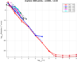
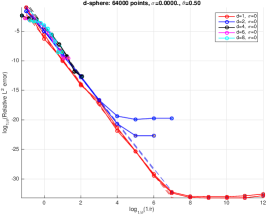
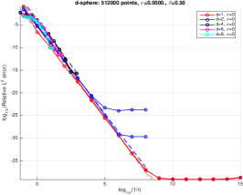
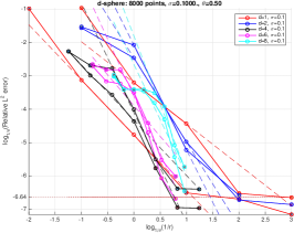
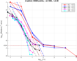
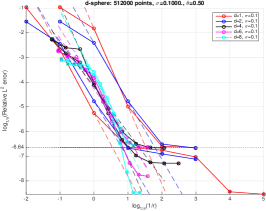
Figure 1: Experiment with $\mathbb{S}^{d}$, without (top row) and with Gaussian noise (bottom row). The columns correspond to different values of $n\in\{8000,64000,512000\}$. In the plots the dots represent the $L^{2}(\Pi)$ error squared (or MSE) of GMRA approximations (see (5)) as a function of the radius $r$ at scale $j$; more precisely the abscissa is in terms of $\log_{2}(1/r_{j})$, where $r_{j}$ is the mean radius of $C_{j,k}$ for a fixed $j$, and the ordinate is $\log_{2}\text{MSE}_{j}$, where $\text{MSE}_{j}$ is the mean squared error of the GMRA approximation at scale $j$. Different colors correspond to different intrinsic dimensions $d$ (see legend). The two cases $D=10,100$ use the same colors for both the dots and the lines, all of which are essentially superimposed since our results are independent of the ambient dimension $D$. For each dimension we fit a line to measure the decay, which is $O(r^{-4})$ independently of $d$, consistently with our analysis. The horizontal dotted line, with corresponding tick mark on the $Y$ axis, represents the noise level $\sigma^{2}$: the approximation error flattens out at roughly that level, as expected.

We considered various settings of the parameters, namely all combinations of: $d\in\{1,2,4,6,8\}$, $n\in\{8000,16000,32000,64000,128000\}$, $D\in\{100,1000\}$, $\sigma\in\{0,0.05,0.1\}$. We only display some of the results for reasons of space constraints.

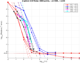
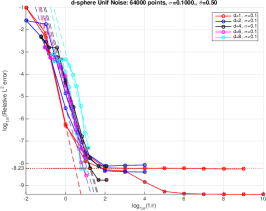
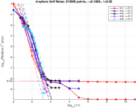
Figure 2: This figure is as the second row of Figure 1, but the noise is radially uniform with widht parameter $\sigma$. Note that the variance of the noise is $\sigma^{2}/3$, which is indicated in the figure by horizontal line and an extra tick mark on the $Y$-axis in the figures. The MSE converges quickly to that level as a function of scale.

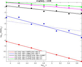
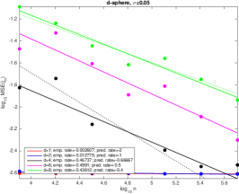
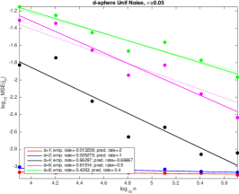
Figure 3: For the example of $\mathbb{S}^{d}$ considered in this section we consider the MSE error, i.e. $L^{2}(\Pi)$ squared error (as defined in (5)) at the optimal scale $j_{n}$ (as in the proof of Corollary 8) as a function of the number of points $n\in\{8000,16000,32000,64000,128000,256000,512000\}$, and compare our empirical rates (solid linear, with the rate reported in the legend under “emp. rate”) with the rates predicted by Corollary 8 (dotted lines, with rate reported in the legend under “pred. rate”), for various choices of the intrinsic dimension $d\in\{1,2,4,6,8\}$ and fixed ambient dimension $D=10$ (the results are independent of $D$, so we do note report the - very similar - results obtained for $D=100$). Left: noiseless case, middle: Gaussian noise, right: radial uniform noise (see text). The rates match our results quite well, except in the case $d=2$ where we seem to obtain the same convergence rate as in the $d=1$ case. Here we are choosing the optimal scale to be the finest scale such that, in every cell, we have at least $10d^{2}$ points. For the noisy cases, the approximation rates for $d=1,2$ are not meaningful simply because we have enough points to go the finest scale above the noise level.

6.2 Meyer’s staircase

We consider the ($d$-dimensional generalization of) Y. Meyer’s staircase. Consider the cube $Q=[0,1]^{d}$ and the set of Gaussians $\mathcal{N}(x;\mu,\delta^{2}I_{d})$ where the mean $\mu$ is allowed to vary over $Q$, and the function is truncated to only accept arguments $x\in Q$. Varying $\mu$ in $Q$ in this manner induces a smooth embedding of a $d$-dimensional manifold into the infinite dimensional Hilbert space $L^{2}(Q)$. That is, the Gaussian density centered at $\mu\in Q$ and truncated to $x\in Q$ is a point in $L^{2}(Q)$. By discretizing $Q$, we may sample this manifold and project it into a finite dimensional space. In particular, a grid $\Gamma_{D}\subseteq Q$ of $D$ points (obtained by subdividing in $D^{-\frac{1}{d}}$ equal parts along each dimension) may be generated and considering the evaluations of the set of translated Gaussians on this grid produces an embedding of this manifold into $\mathbb{R}^{D}$. Sampling $n$ points from this manifold by randomly drawing $\mu_{1},\dots,\mu_{n}$ uniformly from $Q$, we obtain a set $\{\mathcal{N}(x;\mu_{i},\delta^{2}I_{d})|_{\Gamma_{D}}\}_{i=1,\dots,n}$ of $n$ samples from the “discretized” Meyer’s staircase in $\mathbb{R}^{D}$. This is what we call a sample from Meyer’s staircase, which is illustrated in Figure 4. This example is not artificial: for example, translating a white shape on a black background produces a set of $2-D$ images with a similar structure to the $d$-dimensional Meyer’s staircase for $d=2$.

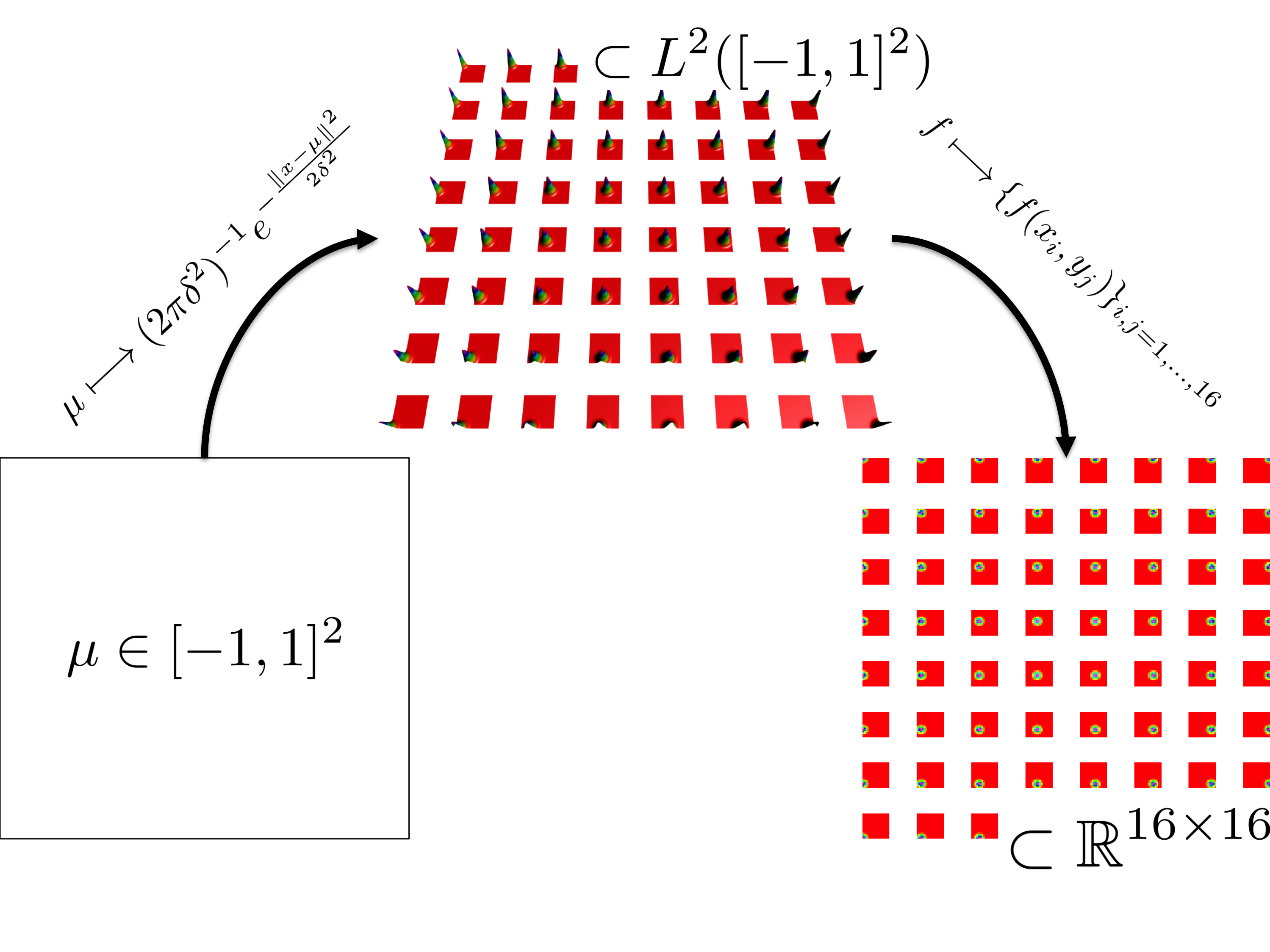
Figure 4: An illustration of Meyer’s staircase for $d=2$. We see that the square is mapped into a subset of $L^{2}([-1,1]^{2})$ consisting of truncated Gaussians. These are then sampled at points on a uniform, $16$ by $16$ grid to obtain an embedding of $[0,1]^{2}$ into $\mathbb{R}^{16\times 16}$. For small $\delta$, this embedding has a point very close to each coordinate axis in $\mathbb{R}^{16\times 16}$. Thus, it comes as no surprise that this embedding of $[-1,1]^{2}$ into $\mathbb{R}^{256}$ has a high degree of curvature.

The manifold associated with Meyer’s staircase is poorly approximated by subspaces of dimension smaller than $O(D\wedge 1/\delta^{D})$, and besides spanning many dimensions in $\mathbb{R}^{D}$, it has a small reach, depending on $d,D,\delta$. In our examples we considered

$$n=8000,16000,32000,640000,128000,\ d=1,2,4,\ D=2000,\text{ and }\delta=\frac{5}{100}.$$

We consider the noiseless case, as well as the case where Gaussian noise $\mathcal{N}(0,\frac{1}{D}I_{D})$ is added to the data. Since this type of noise does not abide by the $(\sigma,\tau)$-model assumption and $\tau$ is very small for Meyer’s staircase, Figure 5 illustrates the behavior of the GMRA approximation outside of the regime where our theory is applicable.

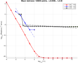
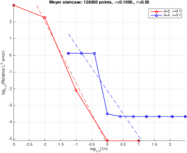
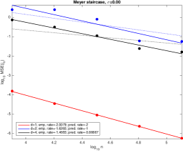
Figure 5: Left and middle: MSE as a function of scale $r$ for the $d$-dimensional Meyer’s staircase, for different values of $n=$, $d$ and $\sigma$, standard deviation of Gaussian noise $\mathcal{N}(0,\frac{\sigma^{2}}{D})$. The small reach of Meyer’s staircase makes it harder to approximate, and makes the approximation much more susceptible to noise. Moreover, Gaussian noise is unbounded, so this distribution violates the $(\sigma,\tau)$-model assumption (albeit only at a small number of points, with high probability). Right: MSE at the optimal scale, chosen so that every cell contains at least $10d^{2}$ points.

6.3 The MNIST dataset of handwritten digits

We consider the MNIST data set of images of handwritten digits, each of size $28\times 28$, grayscale. There are total of $60,000$, from ten classes consisting of digits $0,1,\dots,9$. The intrinsic dimension of this data set is variable across the data, perhaps because different digits have a different number of “degrees of freedom” and across scales, as it is observed in Little et al. (2012). We run GMRA by setting the cover tree scaling parameter $\theta$ equal to $0.9$ (meaning that we replace $1/2$ with $0.9$ in definition of cover trees in section 3.2) in order to slowly “zoom” into the data at multiple scales. As the intrinsic dimension is not well-defined, we set GMRA to pick the dimension of the planes $\mathbb{V}_{j,k}$ adaptively, as the smallest dimension needed to capture half of the “energy” of the data in $C_{j,k}$. The distribution of dimensions of the subspaces $\mathbb{V}_{j,k}$ has median $3$ (consistently with the estimates in Little et al. (2012)) and is represented in figure 6. We then compute the $L^{2}$ relative approximation error, and compute various quantiles: this is reported in the same figure. The running time on a desktop was few minutes.

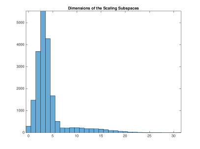
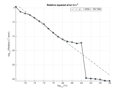
Figure 6: Left: histogram of the dimension of the scaling function subspaces for the MNIST data set. We see that many of the subspaces are very low-dimensional, with dimensions mostly between $2$ and $5$. Right: $L^{2}$ relative approximation error squared as a function of scale. We do not plot the quantiles since many of them are many orders of magnitude smaller (which is a good thing in terms of approximation error), creating artifacts in the plots; they do indicate thought that the structure of the data is highly complex and not heterogeneous. Note that the axis of this plot are in $\log_{1/\theta}$ scale, where $\theta=0.9$ is the cover tree scaling factor used in this example. Note how the approximation error decreases slowly at the beginning, as there are many classes, rather far from each other, so that it takes a few scales before GMRA starts focusing into each class, at which point the approximation error decreases more rapidly. This phenomenon does not happen uniformly over the data (figure not shown).

6.4 Sonata Kreutzer

We consider a recording of the first movement of the Sonata Kreutzer by L.V. Beethoven, played by Y. Pearlman (violin) and V. Ashkenazy (piano) (EMI recordings). The recording is stereo, sampled at 44.1kHz. We map it to mono by simply summing the two audio channels, and then we generate a high-dimensional dataset as follows. We consider windows of width $w$ seconds, overlapping by $\delta w$ seconds, and consider the samples in each such time window $[i\delta w,i\delta w+w)$ as a high-dimensional vector $X^{\prime}_{i}$, of dimension equal to the sampling rate times $w$. In our experiment we choose $w=0.1$ seconds, $\delta w=0.05$ seconds, and the resulting vectors $X^{\prime}_{i}$ are $D^{\prime}=551$-dimensional. Since Euclidean distances between the $X^{\prime}_{i}$ are far from being perceptually relevant, we transform each $X^{\prime}_{i}$ to its cepstrum (see Oppenheim and Schafer (1975)), remove the central low-pass frequency, and discard the symmetric part of the spectrum (the signal is real), obtaining $X_{i}$, a vector with $D=275$ dimensions, and $i$ ranges from $0$ to about $130,000$. The running time on a desktop was few minutes.

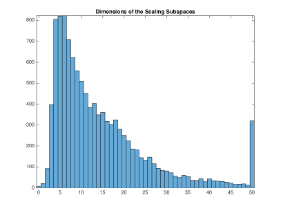
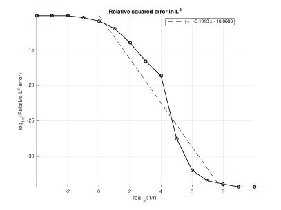
Figure 7: Left: histogram of the dimension of the scaling function subspaces for the Kreutzer sonata dataset. We see that the dimension of the scaling function subspaces is mostly between $4$ and $25$. Right: mean $L^{2}$ relative approximation error squared as a function of scale. We do not plot the quantiles since many of them are many orders of magnitude smaller (which is a good thing in terms of approximation error), creating artifacts in the plots; they do indicate that the structure of the data is highly complex and non-heterogeneous. Note that the axes of this plot are in $\log_{1/\theta}$ scale, where $\theta=0.9$ is the scaling factor used in this example.

Acknowledgments

The authors gratefully acknowledge support from NSF DMS-0847388, NSF DMS-1045153, ATD-1222567, CCF-0808847, AFOSR FA9550-14-1-0033, DARPA N66001-11-1-4002. We would also like to thank Mark Iwen for his insightful comments.

Appendix: Proofs of geometric propositions and lemmas

Proof [Proof of Proposition 10] For the first inequality, let

$$A=\begin{pmatrix}I\\ X\end{pmatrix}\text{ and }B=\begin{pmatrix}Y\\ 0\end{pmatrix},$$

and for every $T\subset[d]$, we let $V_{T}$ denote the volume of $\{a_{i}\}_{i\in T^{c}}\cup\{b_{i}\}_{i\in T}$, where $a_{i}$ and $b_{i}$ denote the $i$th columns of $A$ and $B$ respectively. By submultilinearity of the volume we have

$${\rm Vol}(A+B)\leq\sum_{T\in 2^{[d]}}V_{T},$$

where $2^{[d]}=\{S:S\subset\{1,\ldots,d\}\}$. We now show that $V_{T}\leq q^{|T|}{\rm Vol}(A)$ for every $T\in 2^{[d]}$. The bound $\|Y\|\leq q$ implies $\|y_{i}\|\leq q$ for all $i=1,\ldots,d$, and so the fact that the volume is a submultiplicative function implies that

$$V_{T}\leq q^{|T|}{\rm Vol}(A_{T^{c}}).$$

On the other hand, letting $a_{1}^{\perp}$ be the orthogonal projection of $a_{1}$ onto $\text{span}^{\perp}\{a_{i}\}_{i=2}^{d}$, we note that $\|a_{1}^{\perp}\|\geq 1$, and thus

$${\rm Vol}(A_{\{1\}^{c}})\leq\|a_{1}^{\perp}\|{\rm Vol}(A_{\{1\}^{c}})={\rm Vol}(A).$$

By induction and invariance of the volume under permutations, we see that ${\rm Vol}(A_{T^{c}})\leq{\rm Vol}(A)$ for all $T\in 2^{[d]}$. Thus,

$${\rm Vol}(A+B)\leq\sum_{T\in 2^{[d]}}q^{|T|}{\rm Vol}(A)=(1+q)^{d}{\rm Vol}(A).$$

For the second inequality, since $Y$ is symmetric, we can represent it as $Y=F-G$ where $F$ and $G$ are symmetric positive semidefinite, $FG=GF=0$, and $\|F\|,\|G\|\leq\|Y\|$. Indeed, if $Y=Q\Lambda Q^{T}$ is the eigenvalue decomposition of $Y$ with $\Lambda=\mathop{\rm diag}(\lambda)$, set $\lambda_{+}:=(\max(0,\lambda_{1}),\ldots,\max(0,\lambda_{d}))^{T}$, $\lambda_{-}:=\lambda_{+}-\lambda$, and define $F:=Q\mathop{\rm diag}(\lambda_{+})Q^{T}$, $G=Q\mathop{\rm diag}(\lambda_{-})Q^{T}$.

Recall the matrix determinant lemma: let $T\in\mathbb{R}^{k\times k}$ be invertible, and let $U,V\in\mathbb{R}^{k\times l}$. Then

$${\rm Vol}(T+UV^{T})={\rm Vol}(I+V^{T}T^{-1}U){\rm Vol}(T).$$

Applying it in our case with $U=\begin{pmatrix}\sqrt{F}-\sqrt{G}\\ 0\end{pmatrix}$, $V=\begin{pmatrix}\sqrt{F}+\sqrt{G}\\ 0\end{pmatrix}$, and $T=\begin{pmatrix}I&X^{T}\\ X&-I\end{pmatrix}$, we have that

$${\rm Vol}\begin{pmatrix}I+Y&X^{T}\\ X&-I\\ \end{pmatrix}={\rm Vol}\left(I+\begin{pmatrix}\sqrt{F}+\sqrt{G}\\ 0\end{pmatrix}^{T}\begin{pmatrix}I&X^{T}\\ X&-I\\ \end{pmatrix}^{-1}\begin{pmatrix}\sqrt{F}-\sqrt{G}\\ 0\end{pmatrix}\right){\rm Vol}\begin{pmatrix}I&X^{T}\\ X&-I\\ \end{pmatrix}.$$

By orthogonality of the columns in $\begin{pmatrix}I\\ X\end{pmatrix}$ with the columns in $\begin{pmatrix}X^{T}\\ -I\end{pmatrix},$ we have that

$$\left\|\begin{pmatrix}I&X^{T}\\ X&-I\\ \end{pmatrix}\begin{pmatrix}u\\ v\end{pmatrix}\right\|\geq\left\|\begin{pmatrix}u\\ v\end{pmatrix}\right\|,$$

and hence

$$\left\|\begin{pmatrix}\sqrt{F}+\sqrt{G}\\ 0\end{pmatrix}^{T}\begin{pmatrix}I&X^{T}\\ X&-I\\ \end{pmatrix}^{-1}\begin{pmatrix}\sqrt{F}-\sqrt{G}\\ 0\end{pmatrix}\right\|\leq\sqrt{q}\cdot 1\cdot\sqrt{q}=q.$$

Therefore, we conclude that

$${\rm Vol}\left(I+\begin{pmatrix}\sqrt{F}+\sqrt{G}\\ 0\end{pmatrix}^{T}\begin{pmatrix}I&X^{T}\\ X&-I\\ \end{pmatrix}^{-1}\begin{pmatrix}\sqrt{F}-\sqrt{G}\\ 0\end{pmatrix}\right)\geq(1-q)^{d},$$

and combining this with the expression from the matrix determinant lemma completes the proof.  

Proof [Proof of Lemma 15] Let $\gamma:[0,d_{\mathcal{M}}(z,y)]\rightarrow\mathcal{M}$ denote the arclength-parameterized geodesic connecting $y$ to $z$ in $\mathcal{M}$. Since $\gamma$ is a geodesic, there is a $v\in T_{y}\mathcal{M}$ with $\|v\|=1$ such that the Taylor expansion

$$z=y+d_{\mathcal{M}}(z,y)v+\int_{0}^{d_{\mathcal{M}}(z,y)}\gamma^{\prime\prime}(t)\left(d_{\mathcal{M}}(z,y)-t\right)dt.$$

By Proposition 11, $\|\gamma^{\prime\prime}(t)\|_{2}\leq 1/\tau$ for all $t$ and $d_{\mathcal{M}}(z,y)\leq 2r$, so we have that

$$|\langle\eta,z-y\rangle| =\left|\left\langle\eta,\int_{0}^{d_{\mathcal{M}}(z,y)}\gamma^{\prime\prime}(t)\left(d_{\mathcal{M}}(z,y)-t\right)dt\right\rangle\right|$$

$$\leq\int_{0}^{d_{\mathcal{M}}(z,y)}|\langle\eta,\gamma^{\prime\prime}(t)\rangle|\left(d_{\mathcal{M}}(z,y)-t\right)dt$$

$$\leq\frac{1}{\tau}\int_{0}^{d_{\mathcal{M}}(z,y)}\left(d_{\mathcal{M}}(z,y)-t\right)dt$$

$$\leq\frac{d_{\mathcal{M}}(z,y)^{2}}{2\tau}$$

$$\leq\frac{2r^{2}}{\tau}.$$

 

Proof [Proof of Lemma 16] Suppose $a$ and $b$ are distinct in $B(y,r)\cap{\mathcal{M}}$. Now, $b-a=v+w$ where $v\in T_{a}\mathcal{M}$ and $w\in T_{a}^{\perp}\mathcal{M}$, and note that $\|w\|\leq\frac{2\|b-a\|^{2}}{\tau}\leq 4\frac{r}{\tau}$ by Lemma 15. This also implies that

$$\|v\| =\sqrt{\|a-b\|^{2}-\|w\|^{2}}\geq\sqrt{\|a-b\|^{2}-4\frac{\|a-b\|^{4}}{\tau^{2}}}\geq\|a-b\|\sqrt{1-16\frac{r^{2}}{\tau^{2}}}\geq\|a-b\|\sqrt{1-4\frac{r}{\tau}}\,.$$

By part iii. of Proposition 11, there is a $u\in T_{y}\mathcal{M}$ such that $\langle u,v\rangle\geq\|v\|\cos(\phi)$ where $\phi$ is the angle between $T_{y}\mathcal{M}$ and $T_{a}\mathcal{M}$. Then

$$|\langle u,b-a\rangle| \geq|\langle u,v\rangle|-|\langle u,w\rangle|$$

$$\geq\|v\|\cos(\phi)-\|w\|$$

$$\geq\|a-b\|\sqrt{1-4\frac{r}{\tau}}\sqrt{1-2\frac{r}{\tau}}-2\frac{\|a-b\|^{2}}{\tau}$$

$$\geq\|b-a\|\left(\sqrt{1-4\frac{r}{\tau}}\sqrt{1-4\frac{r}{\tau}}-4\frac{r}{\tau}\right)$$

$$\geq\|b-a\|\left(1-8\frac{r}{\tau}\right).$$

It then follows from $r<\tau/8$ that $\mathop{{\rm Proj}}{}_{T_{y}\mathcal{M}}(b-a)\not=0$, and hence $\mathop{{\rm Proj}}{}_{y+T_{y}\mathcal{M}}(a)\not=\mathop{{\rm Proj}}{}_{y+T_{y}\mathcal{M}}(b)$ and injectivity holds.  

Proof [Proof of Proposition 17] For $\varepsilon<\tau/8$, we may define the embedding

$$\begin{pmatrix}v\\ \beta\end{pmatrix}\longmapsto\begin{pmatrix}v\\ f(v)\end{pmatrix}+\begin{pmatrix}Df(v)^{T}\\ -I\\ \end{pmatrix}\beta$$

where we have assumed (without loss of generality) that $y=0$ and $T_{y}\mathcal{M}$ coincides with the span of the first $d$ canonical orthonormal basis members. The domain of this map is the set

$$\Omega=\{(v,\beta)\in\mathbb{R}^{d}\times\mathbb{R}^{D-d}:v\in T_{y}\mathcal{M}\cap B(0,\varepsilon),\|\beta\|^{2}+\|Df(v)^{T}\beta\|^{2}<\tau^{2}\}$$

and the Jacobian of this map is

$$\begin{pmatrix}I+\sum_{i=1}^{D-d}\beta_{i}D^{2}f_{i}(v)&Df(v)^{T}\\ Df(v)&-I\end{pmatrix}.$$

It is clear that the inverse of the above map is given by

$$x\longmapsto(\mathop{{\rm Proj}}{}_{y+T_{y}\mathcal{M}}(\mathop{{\rm Proj}}{}_{\mathcal{M}}(x)),\mathop{{\rm Proj}}{}_{T_{y}^{\perp}\mathcal{M}}(x-\mathop{{\rm Proj}}{}_{\mathcal{M}}(x))),$$

which is at least a $C^{1}$ map. Thus, a necessary condition for the $\tau$-radius normal bundle to embed is that the Jacobian exhibited above is invertible, which in turn implies that

$$\begin{pmatrix}I+\sum_{i=1}^{D-d}\beta_{i}D^{2}f_{i}(v)&Df(v)^{T}\\ Df(v)&-I\end{pmatrix}\begin{pmatrix}\zeta\\ Df(v)\zeta\end{pmatrix}\not=0$$

for all $\zeta\not=0$ when $(v,\beta)\in\Omega$. This reduces to $(I+\sum\beta_{i}D^{2}f_{i}(v)+Df(v)^{T}Df(v))\zeta\not=0$, and so a necessary condition for embedding is then that the norm of $\sum_{i=1}^{D-d}\beta_{i}D^{2}f_{i}(v)$ does not exceed $1+\|Df(v)\|^{2}$ whenever

$$\left\|\begin{pmatrix}Df(v)^{T}\\ -I\end{pmatrix}\beta\right\|^{2}=\|\beta\|^{2}+\|Df(v)^{T}\beta\|^{2}<\tau^{2}.$$

In particular, this must be true if $\|\beta\|<\tau/\sqrt{1+\|Df(v)\|^{2}}$. This reduces to the condition that the operator norm

$$\sup_{u\in\mathcal{S}^{D-d-1}}\left\|\sum_{i=1}^{D-d}u_{i}D^{2}f_{i}(v)\right\|<\frac{(1+\|Df(v)\|^{2})^{3/2}}{\tau}<\frac{1}{\tau}\left(1+\|Df(v)\|\right)^{3}.$$ (28)

By the fundamental theorem of calculus, we have that

$$Df(v)x=Df(0)x+\int_{0}^{\|v\|}[u_{v}^{T}D^{2}f_{i}(tu_{v})x]dt=\int_{0}^{\|v\|}[u_{v}^{T}D^{2}f_{i}(tu_{v})x]dt,$$

where $u_{v}=v/\|v\|$ and $[u_{v}^{T}D^{2}f_{i}(tu_{v})x]$ indicates a vector with $i$th component $u_{v}^{T}D^{2}f_{i}(tu_{v})x$. Consequently, for any $x\in\mathbb{R}^{d}$, we have that

$$\|Df(v)x\| \leq\int_{0}^{\|v\|}\left\|[u_{v}^{T}D^{2}f_{i}(tu_{v})x]\right\|dt\leq\|v\|\sup_{t\in[0,\|v\|]}\left\|[u_{v}^{T}D^{2}f_{i}(tu_{v})x]\right\|$$ (29)

$$\leq\varepsilon\sup_{t\in[0,\varepsilon]}\left\|[u_{v}^{T}D^{2}f_{i}(tu_{v})x]\right\|.$$

Now,

$$\left\|[u_{v}^{T}D^{2}f_{i}(tu_{v})x]\right\| =\sup_{u\in\mathcal{S}^{D-d-1}}\langle u,[u_{v}^{T}D^{2}f_{i}(tu_{v})x]\rangle=\sup_{u\in\mathcal{S}^{D-d-1}}\sum_{i=1}^{D-d}u_{i}(u_{v}^{T}D^{2}f_{i}(tu_{v})x)$$

$$=\sup_{u\in\mathcal{S}^{D-d-1}}u_{v}^{T}\left(\sum_{i=1}^{D-d}u_{i}D^{2}f_{i}(tu_{v})\right)x$$

$$\leq\sup_{u\in\mathcal{S}^{D-d-1}}\|u_{v}\|\left\|\sum_{i=1}^{D-d}u_{i}D^{2}f_{i}(tu_{v})\right\|\|x\|$$

$$=\|x\|\sup_{u\in\mathcal{S}^{D-d-1}}\left\|\sum_{i=1}^{D-d}u_{i}D^{2}f_{i}(tu_{v})\right\|,$$

which together with (29) and (28) yields the bound

$$\|Df(v)\|<\frac{\varepsilon}{\tau}\left(1+\sup_{t\in[0,\varepsilon]}\|Df(tu_{v})\|\right)^{3}.$$

Since this inequality also holds for any $v^{\prime}$ with $\|v\|\leq\varepsilon^{\prime}$, taking a supremum yields

$$\sup_{\varepsilon^{\prime}\in[0,\varepsilon]}\|Df(tu_{v})\| \leq\sup_{\varepsilon^{\prime}\in[0,\varepsilon]}\frac{\varepsilon^{\prime}}{\tau}\left(1+\sup_{t\in[0,\varepsilon^{\prime}]}\|Df(tu_{v})\|\right)^{3}\leq\frac{\varepsilon}{\tau}\left(1+\sup_{\varepsilon^{\prime}\in[0,\varepsilon]}\|Df(tu_{v})\|\right)^{3},$$

and hence

$$\sup_{v\in B_{d}(0,\varepsilon)}\|Df(v)\|\leq\frac{\varepsilon}{\tau}\left(1+\sup_{v\in B_{d}(0,\varepsilon)}\|Df(v)\|\right)^{3}.$$

Setting $a(\varepsilon^{\prime})=\sup_{v\in B_{d}(0,\varepsilon^{\prime})}\|Df(v)\|$, we have that $a(0)=0$,

$$a(\varepsilon^{\prime})\leq\frac{\varepsilon^{\prime}}{\tau}\left(1+a(\varepsilon^{\prime})\right)^{3},$$

for all $\varepsilon^{\prime}\geq 0$, and $a$ is continuous by continuity of $\|Df(v)\|$. Setting $b(\varepsilon^{\prime})=a(\varepsilon^{\prime})/(1+a(\varepsilon^{\prime}))$, we get

$$b(\varepsilon^{\prime})(1-b(\varepsilon^{\prime}))^{2}\leq\frac{\varepsilon^{\prime}}{\tau}.$$

Examining the polynomial $x(1-x)^{2}$, we see that the sublevel set $x(1-x)^{2}\leq\omega$ consists of two components when $\omega<4/27$. Also note that if $\omega<1/8$, then

$$2(1-2\omega)^{2}=2-8\omega+8\omega^{2}>2-1=1,$$

and hence

$$2\omega(1-2\omega)^{2}>\omega.$$

Consequently, if $x$ is such that $x(1-x)^{2}\leq\omega$ and is in the interval containing zero in the sublevel set $x(1-x)^{2}\leq\omega<1/8$, then $x\leq 2\omega$.

By these observations, continuity of $b(\varepsilon^{\prime})$, and the fact that $b(0)=0$, we have that $a(\varepsilon^{\prime})\leq\frac{2\frac{\varepsilon^{\prime}}{\tau}}{1-2\frac{\varepsilon^{\prime}}{\tau}}$, and thus

$$\sup_{v\in B_{d}(0,\varepsilon)}\|Df(v)\|\leq\frac{2\varepsilon}{\tau-2\varepsilon}.$$

From the bound in (28) we now acquire the bound

$$\sup_{v\in B_{d}(0,\varepsilon)}\sup_{u\in\mathcal{S}^{D-d-1}}\left\|\sum_{i=1}^{D-d-1}u_{i}D^{2}f_{i}(v)\right\|\leq\frac{\tau^{2}}{(\tau-2\varepsilon)^{3}}.$$

 

Proof [Proof of Lemma 18] We first prove part i. Let $\varepsilon>0$ satisfy $\varepsilon<\tau/8$. Because of (23) and the fact that $\|\beta\|\leq\sigma$, we have that

$$\left\|\sum_{i=1}^{D-d}\beta_{i}D^{2}f_{i}(v)\right\|\leq\frac{\sigma\tau^{2}}{(\tau-2\varepsilon)^{3}}.$$

Since this is also a bound for the columns of $\sum\beta_{i}D^{2}f_{i}(v)$, Proposition 10 implies that

$$\text{Vol}\begin{pmatrix}I+\sum\beta_{i}D^{2}f_{i}(v)&Df(v)^{T}\\ Df(v)&-I\end{pmatrix} \leq\left(1+\frac{\sigma\tau^{2}}{(\tau-2\varepsilon)^{3}}\right)^{d}{\rm Vol}\begin{pmatrix}I&Df(v)^{T}\\ Df(v)&-I\end{pmatrix}$$

in $T^{\perp}(\mathcal{M}\cap B(y,\varepsilon))\cap\mathcal{M}_{\sigma}$.

On the other hand, we have that

$${\rm Vol}\begin{pmatrix}Df^{T}(v)\\ -I\end{pmatrix}\leq\prod_{i=1}^{D-d}\sqrt{1+\|\nabla f_{i}(v)\|^{2}}\leq\left(1+\frac{4\varepsilon^{2}}{(\tau-2\varepsilon)^{2}}\right)^{(D-d)/2}$$

since (22) implies the bounds $\|\frac{\partial f(v)}{\partial v_{i}}\|\leq\frac{2\varepsilon}{\tau-2\varepsilon}$ for each $i=1,\ldots,d$, and the above is the largest this quantity may be subject to these bounds.

When these estimates are joined together, we have an inequality

$${\rm Vol}\begin{pmatrix}I+\sum_{i=1}^{D-d}\beta_{i}D^{2}f_{i}(v)&Df(v)^{T}\\ Df(v)&-I\end{pmatrix} \leq\left(1+\frac{\sigma\tau^{2}}{(\tau-2\varepsilon)^{3}}\right)^{d}\text{Vol}\begin{pmatrix}I&Df(v)^{T}\\ Df(v)&-I\end{pmatrix}$$

$$\leq\left(1+\frac{\sigma\tau^{2}}{(\tau-2\varepsilon)^{3}}\right)^{d}\left(1+\frac{4\varepsilon^{2}}{(\tau-2\varepsilon)^{2}}\right)^{(D-d)/2}{\rm Vol}\begin{pmatrix}I\\ Df(v)\end{pmatrix}.$$

For an arbitrarily small $\varepsilon>0$, let $\{U_{\gamma}\}_{\gamma\in\Gamma}$ denote a finite partition of $U$ into measurable sets such that there for each $\gamma\in\Gamma$, there is a $y_{\gamma}$ satisfying $U_{\gamma}\subset\mathcal{M}\cap B(y_{\gamma},\varepsilon)$. Let $f_{\gamma}$ denote the inverse of $P_{\gamma}=\mathop{{\rm Proj}}{}_{y_{\gamma}+T_{y_{\gamma}}\mathcal{M}}$ in $U_{\gamma}$, and set

$$E_{\gamma,v}=\{\beta\in\mathbb{R}^{D-d}:\|\beta\|^{2}+\|Df_{\gamma}(v)\beta\|^{2}\leq\sigma^{2}\}$$

for all $v\in P_{\gamma}(U_{\gamma})$. Thus,

$$\int_{P_{\gamma}^{-1}(U_{\gamma})}d{\rm Vol}(x) =\int_{P_{\gamma}(U_{\gamma})}\int_{E_{\gamma,v}}{\rm Vol}\begin{pmatrix}I+\sum_{i=1}^{D-d}\beta_{i}D^{2}f_{i}(v)&Df(x)^{T}\\ Df(v)&-I\end{pmatrix}d\beta dv$$

$$\leq\int_{P_{\gamma}(U_{\gamma})}\int_{E_{\gamma,v}}\left(1+\frac{\sigma\tau^{2}}{(\tau-2\varepsilon)^{3}}\right)^{d}\left(1+\frac{4\varepsilon^{2}}{(\tau-2\varepsilon)^{2}}\right)^{(D-d)/2}{\rm Vol}\begin{pmatrix}I\\ Df(v)\end{pmatrix}d\beta dv$$

$$\leq\left(1+\frac{\sigma\tau^{2}}{(\tau-2\varepsilon)^{2}}\right)^{d}\left(1+\frac{4\varepsilon^{2}}{(\tau-2\varepsilon)^{2}}\right)^{(D-d)/2}\mathop{\rm Vol}{}_{\mathcal{M}}(U_{\gamma}){\rm Vol}(B_{D-d}(0,\sigma))$$

since $E_{\gamma,v}\subset B_{D-d}(0,\sigma)$. Consequently, we have that

$${\rm Vol}(P^{-1}(U)) =\sum_{\gamma\in\Gamma}{\rm Vol}(P_{\gamma}^{-1}(U_{\gamma}))$$

$$\leq\sum_{\gamma\in\Gamma}\left(1+\frac{\sigma\tau^{2}}{(\tau-2\varepsilon)^{3}}\right)^{d}\left(1+\frac{4\varepsilon^{2}}{(\tau-2\varepsilon)^{2}}\right)^{(D-d)/2}\mathop{\rm Vol}{}_{\mathcal{M}}(U_{\gamma}){\rm Vol}(B_{D-d}(0,\sigma))$$

$$=\left(1+\frac{\sigma\tau^{2}}{(\tau-2\varepsilon)^{3}}\right)^{d}\left(1+\frac{4\varepsilon^{2}}{(\tau-2\varepsilon)^{2}}\right)^{(D-d)/2}\mathop{\rm Vol}{}_{\mathcal{M}}(U){\rm Vol}(B_{D-d}(0,\sigma)).$$

Since $\varepsilon>0$ was arbitrary, we obtain

$${\rm Vol}(P^{-1}(U))\cap\mathcal{M}_{\sigma})\leq\left(1+\frac{\sigma}{\tau}\right)^{d}\mathop{\rm Vol}{}_{\mathcal{M}}(U){\rm Vol}(B_{D-d}(0,\sigma)).$$

This completes the proof of upper bound in part i. Using a similar partition strategy, we have that

$$\int_{P_{\gamma}^{-1}(U_{\gamma})}d{\rm Vol}(x) =\int_{P_{\gamma}(U_{\gamma})}\int_{E_{\gamma,v}}{\rm Vol}\begin{pmatrix}I+\sum_{i=1}^{D-d}\beta_{i}D^{2}f_{i}(v)&Df(x)^{T}\\ Df(v)&-I\end{pmatrix}d\beta dv$$

$$\geq\int_{P_{\gamma}(U_{\gamma})}\int_{E_{\gamma,v}}\left(1-\frac{\sigma\tau^{2}}{(\tau-2\varepsilon)^{3}}\right)^{d}{\rm Vol}\begin{pmatrix}I&Df(v)^{T}\\ Df(v)&-I\end{pmatrix}d\beta dv$$

$$=\int_{P_{\gamma}(U_{\gamma})}\int_{E_{\gamma,v}}\left(1-\frac{\sigma\tau^{2}}{(\tau-2\varepsilon)^{3}}\right)^{d}{\rm Vol}\begin{pmatrix}I\\ Df(v)\end{pmatrix}{\rm Vol}\begin{pmatrix}Df(v)^{T}\\ -I\end{pmatrix}d\beta dv$$

$$\geq\int_{P_{\gamma}(U_{\gamma})}\int_{E_{\gamma,v}}\left(1-\frac{\sigma\tau^{2}}{(\tau-2\varepsilon)^{3}}\right)^{d}{\rm Vol}\begin{pmatrix}I\\ Df(v)\end{pmatrix}d\beta dv$$

$$\geq\int_{P_{\gamma}(U_{\gamma})}\int_{B_{D-d}\left(0,\frac{\sigma}{1+\frac{\varepsilon}{\tau-\varepsilon}}\right)}\left(1-\frac{\sigma\tau^{2}}{(\tau-2\varepsilon)^{3}}\right)^{d}{\rm Vol}\begin{pmatrix}I\\ Df(v)\end{pmatrix}d\beta dv$$

$$=\left(1-\frac{\sigma\tau^{2}}{(\tau-2\varepsilon)^{3}}\right)^{d}\mathop{\rm Vol}{}_{\mathcal{M}}(U_{\gamma}){\rm Vol}\left(B_{D-d}\left(0,\left(1-\frac{\varepsilon}{\tau}\right)\sigma\right)\right)$$

In the inequalities above, we have used the fact that there is a ball of radius $\left(1-\frac{\varepsilon}{\tau}\right)\sigma$ inside of $E_{\gamma,v}$ for each $\gamma$ and each $v$. Aggregating all of the sums and letting $\varepsilon\to 0$ yields the lower bound in part i.

We now prove part ii. Note that

$${\rm Vol}(\mathcal{M}_{\sigma}\cap B(y,r))\leq{\rm Vol}(P^{-1}(\mathcal{M}\cap B(y,r+\sigma)))$$

since $\|\mathop{{\rm Proj}}{}_{\mathcal{M}}(x)-y\|\leq\|x-y\|+\|\mathop{{\rm Proj}}{}_{\mathcal{M}}(x)-x\|\leq r+\sigma$. Part ii. now follows from part i. and the fact that

$$\mathop{\rm Vol}{}_{\mathcal{M}}(\mathcal{M}\cap B(y,r+\sigma)) \leq\int\limits_{P(\mathcal{M}\cap B(y,r+\sigma))}{\rm Vol}\begin{pmatrix}I\\ Df(v)\end{pmatrix}dv$$

$$\leq\left(1+\left(\frac{2(r+\sigma)}{\tau-2(r+\sigma)}\right)^{2}\right)^{d/2}{\rm Vol}(B_{d}(0,r+\sigma)).$$

 

Proof [Proof of Lemma 20] By the variational characterization of eigenvalues, we have that

$$\sum_{i=d+1}^{D}\lambda_{i}(\Sigma) =\mathop{\rm argmin~{}}_{\dim(V)=D-d}{\rm tr\,}(\mathop{{\rm Proj}}{}_{V}^{T}\Sigma\mathop{{\rm Proj}}{}_{V})$$

$$=\mathop{\rm argmin~{}}_{\dim(V)=D-d}\mathbb{E}\|\mathop{{\rm Proj}}{}_{V}(Z-\mathbb{E}Z)\|^{2}$$

$$=\mathop{\rm argmin~{}}_{\dim(V)=d}\mathbb{E}\|Z-\mathbb{E}Z-\mathop{{\rm Proj}}{}_{V}(Z-\mathbb{E}Z)\|^{2}.$$

Thus, we have that $\sum\limits_{i=d+1}^{D}\lambda_{i}(\Sigma)\leq\mathbb{E}\|Z-\mathbb{E}Z-\mathop{{\rm Proj}}{}_{T_{y}\mathcal{M}}(Z-\mathbb{E}Z)\|^{2}$. Observe that

$$\mathbb{E}\|Z-\mathbb{E}Z-\mathop{{\rm Proj}}{}_{T_{y}\mathcal{M}}(Z-\mathbb{E}Z)\|^{2}= \mathbb{E}\|Z-y+(y-\mathbb{E}Z)-\mathop{{\rm Proj}}{}_{T_{y}\mathcal{M}}((Z-y)+(y-\mathbb{E}Z))\|^{2}$$

$$= \mathbb{E}\|Z-y-\mathop{{\rm Proj}}{}_{T_{y}\mathcal{M}}(Z-y)\|^{2}$$

$$-\|(y-\mathbb{E}Z)-\mathop{{\rm Proj}}{}_{T_{y}\mathcal{M}}(y-\mathbb{E}Z)\|^{2}$$

$$\leq\mathbb{E}\|Z-y-\mathop{{\rm Proj}}{}_{T_{y}\mathcal{M}}(Z-y)\|^{2}.$$

Now for any $z\in\mathcal{M}_{\sigma}\cap B(y,r)$, we have that $z=\beta+x$ where $x\in\mathcal{M}$, and $\beta\in T_{x}^{\perp}\mathcal{M}$ satisfies $\|\beta\|\leq\sigma$. Moreover, there is a unique decomposition $x=\eta+v+y$ where $\eta\in T_{y}^{\perp}\mathcal{M}$ and $v\in T_{y}\mathcal{M}$. Thus,

$$\|z-y-\mathop{{\rm Proj}}{}_{T_{y}\mathcal{M}}(z-y)\|=\|\beta+\eta-\mathop{{\rm Proj}}{}_{T_{y}\mathcal{M}}\beta\|\leq\|\beta-\mathop{{\rm Proj}}{}_{T_{y}\mathcal{M}}(\beta)\|+\|\eta\|\leq\sigma+\frac{2r^{2}}{\tau},$$ (30)

by Lemma 15, and we obtain the bound

$$\mathbb{E}\|Z-\mathbb{E}Z-\mathop{{\rm Proj}}{}_{T_{y}\mathcal{M}}(Z-\mathbb{E}Z)\|^{2}\leq 2\sigma^{2}+\frac{8r^{4}}{\tau^{2}}.$$ (31)

This establishes the required estimate.  

Proof [Proof of Lemma 21] For any unit vector $u\in T_{y}\mathcal{M}$ we have

$$\mathbb{E}\langle u,Z-\mathbb{E}Z\rangle^{2} =\frac{1}{{\rm Vol}(Q\cap\mathcal{M}_{\sigma})}\int_{Q\cap\mathcal{M}_{\sigma}}\langle u,Z-\mathbb{E}Z\rangle^{2}d{\rm Vol}(Z)$$

$$\geq\frac{1}{{\rm Vol}(B(y,r_{2})\cap\mathcal{M}_{\sigma})}\int_{B(y,r_{1})\cap\mathcal{M}_{\sigma}}\langle u,(Z-y)-\mathbb{E}(Z-y)\rangle^{2}d{\rm Vol}(Z)$$

using the inclusion assumptions, and by adding and subtracting the constant vector $y$.

We now seek to reduce the domain of integration and perform a change of variables. Since $r_{1}\leq\tau/8$, the inverse of the affine projection onto $y+T_{y}\mathcal{M}$ is injective. Without loss of generality, we assume $y=0$ and $T_{y}\mathcal{M}$ is the span of the first $d$ standard orthonormal vectors. Letting $f$ denote the inverse of the affine projection onto $y+T_{y}\mathcal{M}$, we see that the map

$$\begin{pmatrix}v\\ \beta\end{pmatrix}\longmapsto\begin{pmatrix}v\\ f(v)+\beta\end{pmatrix}$$

is well-defined and injective on $\mathop{{\rm Proj}}{}_{T_{y}\mathcal{M}}(\mathcal{M}\cap B(y,r_{1}-\sigma))\times(T_{y}^{\perp}\mathcal{M}\cap B(0,\sigma))$. Let $g$ denote this map, note that

$$\|x+\beta\|\leq\|x\|+\|\beta\|\leq(r-\sigma)+\sigma=r,$$

for $x\in\mathcal{M}\cap B(y,r_{1}-\sigma)$, and hence the image of $g$ is contained in $\mathcal{M}_{\sigma}\cap B(y,r_{1})$. Since the absolute value of the determinant of the Jacobian of $g$ is always $1$ (it is lower triangular with ones on the diagonal), employing the change of coordinates in the reduced domain of integration yields

$$\mathbb{E}\langle u,Z-\mathbb{E}Z\rangle^{2}\geq\frac{1}{{\rm Vol}(B(y,r_{2})\cap\mathcal{M}_{\sigma})}\int_{\mathcal{A}}\int_{\mathcal{B}}\left\langle\begin{pmatrix}u\\ 0\end{pmatrix},\begin{pmatrix}v\\ f(v)+\beta\end{pmatrix}-\mathbb{E}(Z-y)\right\rangle^{2}d\beta dv,$$

where

$$\mathcal{A}=\mathop{{\rm Proj}}{}_{T_{y}\mathcal{M}}(B(y,r_{1}-\sigma)\cap\mathcal{M}),\>\mathcal{B}=T_{y}^{\perp}\mathcal{M}\cap B(0,\sigma).$$

Note that $B(y,\cos(\theta)(r_{1}-\sigma))\cap(y+T_{y}\mathcal{M})\subset\mathcal{A}$. Setting ${\mathcal{Q}}=\mathop{{\rm Proj}}{}_{T_{y}\mathcal{M}}$, this immediately reduces to

$$\mathbb{E}\langle u,Z-\mathbb{E}Z\rangle^{2} \geq\frac{1}{{\rm Vol}(B(y,r_{2})\cap\mathcal{M}_{\sigma})}\int_{\mathcal{A}}\int_{\mathcal{B}}\langle u,v-\mathbb{E}{\mathcal{Q}}(Z-y)\rangle^{2}d\beta dv$$

$$=\frac{{\rm Vol}(B_{D-d}(0,\sigma))}{{\rm Vol}(B(y,r_{2})\cap\mathcal{M}_{\sigma})}\int_{\mathcal{A}}\langle u,v-\mathbb{E}{\mathcal{Q}}(Z-y)\rangle^{2}dv$$

$$\geq\frac{{\rm Vol}(B_{D-d}(0,\sigma))}{{\rm Vol}(B(y,r_{2})\cap\mathcal{M}_{\sigma})}\int_{B_{d}(0,q)}\langle u,v-\mathbb{E}{\mathcal{Q}}(Z-y)\rangle^{2}dv,$$

where $q=\cos(\delta)(r_{1}-\sigma)$ and $\delta=\arcsin((r_{1}-\sigma)/2\tau)$. Noting that $\int_{B_{d}(0,q)}\langle u,v\rangle dv=0$ by symmetry, we now use linearity of the inner product to further reduce the integrand:

$$\mathbb{E}\langle u,Z-\mathbb{E}Z\rangle^{2} \geq\frac{{\rm Vol}(B_{D-d}(0,\sigma))}{{\rm Vol}(B(y,r_{2})\cap\mathcal{M}_{\sigma})}\int_{B_{d}(0,q)}\left(\langle u,v\rangle^{2}-2\langle u,v\rangle\langle u,\mathbb{E}{\mathcal{Q}}(Z-y)\rangle+\langle u,\mathbb{E}{\mathcal{Q}}(Z-y)\rangle^{2}\right)dv$$

$$=\frac{{\rm Vol}(B_{D-d}(0,\sigma))}{{\rm Vol}(B(y,r_{2})\cap\mathcal{M}_{\sigma})}\int_{B_{d}(0,q)}\left(\langle u,v\rangle^{2}+\langle u,\mathbb{E}{\mathcal{Q}}(Z-y)\rangle^{2}\right)dv$$

$$\geq\frac{{\rm Vol}(B_{D-d}(0,\sigma))}{{\rm Vol}(B(y,r_{2})\cap\mathcal{M}_{\sigma})}\int_{B_{d}(0,q)}\langle u,v\rangle^{2}dv$$

$$=\frac{{\rm Vol}(B_{D-d}(0,\sigma)){\rm Vol}(B_{d}(0,q))}{{\rm Vol}(B(y,r_{2})\cap\mathcal{M}_{\sigma})}\frac{q^{2}}{d}.$$

By Lemma 18, we then obtain

$$\mathbb{E}\langle u,Z-\mathbb{E}Z\rangle^{2} \geq\left(\left(1+\frac{\sigma}{\tau}\right)\sqrt{1+\left(\frac{2(r_{2}+\sigma)}{\tau-2(r_{2}+\sigma)}\right)^{2}}\right)^{-d}\frac{{\rm Vol}(B_{d}(0,q))}{{\rm Vol}(B_{d}(0,r_{2}+\sigma))}\frac{q^{2}}{d}$$

$$\geq\frac{1}{4\left(1+\frac{\sigma}{\tau}\right)^{d}}\left(\frac{r_{1}-\sigma}{r_{2}+\sigma}\right)^{d}\left(\frac{1-\left(\frac{r_{1}-\sigma}{2\tau}\right)^{2}}{1+\left(\frac{2(r_{2}+\sigma)}{\tau-2(r_{2}+\sigma)}\right)^{2}}\right)^{d/2}\frac{(r_{1}-\sigma)^{2}}{d}.$$ (32)

Let $V_{d-1}(\Sigma)$ be a subspace corresponding to the first $d-1$ principal components of $Z$:

$$V_{d-1}=\mathop{\rm argmin~{}}_{\dim(V)=d-1}\mathbb{E}\|Z-\mathbb{E}Z-\mathop{{\rm Proj}}{}_{V}(Z-\mathbb{E}Z)\|,$$

and note that $\lambda_{d}(\Sigma)=\max_{0\neq u\in V_{d-1}^{\perp}}\mathbb{E}\left\langle\frac{u}{\|u\|},Z-\mathbb{E}Z\right\rangle^{2}$. Since $\dim(V_{d-1}^{\perp})=D-d+1$ and $\dim(T_{y}\mathcal{M})=d$, it is easy to see that $V_{d-1}^{\perp}\cap T_{y}\mathcal{M}\neq\emptyset.$ For any $u_{\ast}\in V_{d-1}^{\perp}\cap T_{y}\mathcal{M}$ such that $\|u_{\ast}\|=1$ it follows from Courant-Fischer characterization of $\lambda_{d}(\Sigma)$ that

$$\lambda_{d}(\Sigma)\geq\mathbb{E}\left\langle u_{\ast},Z-\mathbb{E}Z\right\rangle^{2},$$

and (Appendix: Proofs of geometric propositions and lemmas) implies the desired bound.  

Proof [Proof of Lemma 22] Let $Q\subset\mathbb{R}^{D}$ be such that $B(y,r_{1})\subset Q$ and $\mathcal{M}_{\sigma}\cap Q\subset B(y,r_{2})$ for some $y\in\mathcal{M}$ and $\sigma<r_{1}<r_{2}<\tau/8-\sigma$. Assume that $Z$ is drawn from $U_{\mathcal{M}_{\sigma}\cap Q}$, let $\Sigma$ be the covariance matrix of $Z$ and $V_{d}:=V_{d}(\Sigma)$ - the subspace corresponding to the first $d$ principal components of $Z$.

Let $\alpha\in[0,1]$ be such that $\cos(\phi):=\min_{u\in V_{d},\|u\|=1}\max_{v\in T_{y}\mathcal{M},\|v\|=1}\left|\left\langle u,v\right\rangle\right|=\sqrt{1-\alpha^{2}}$ is the cosine of the angle between $T_{y}\mathcal{M}$ and $V_{d}$. Then there exists a unit vector $u_{\ast}\in(V_{d})^{\perp}$ such that

$$\max_{v\in T_{y}\mathcal{M},\|v\|=1}|\left\langle u_{\ast},v\right\rangle|\geq\alpha.$$

Indeed, let $u^{\prime}\in V_{d},\ v^{\prime}\in T_{y}\mathcal{M}$ be unit vectors such that $\cos(\phi)=\left\langle u^{\prime},v^{\prime}\right\rangle$, Note that $\sqrt{1-\alpha^{2}}$ is equal to the smallest absolute value among the nonzero singular values of the operator $\mathop{{\rm Proj}}{}_{T_{y}\mathcal{M}}\mathop{{\rm Proj}}{}_{V_{d}}$. Since the spectra of the operators $\mathop{{\rm Proj}}{}_{T_{y}\mathcal{M}}\mathop{{\rm Proj}}{}_{V_{d}}$ and $\mathop{{\rm Proj}}{}_{V_{d}}\mathop{{\rm Proj}}{}_{T_{y}\mathcal{M}}$ coincide by well-known facts from linear algebra, we have that

$$\min_{u\in V_{d},\|u\|=1}\max_{v\in T_{y}\mathcal{M},\|v\|=1}\left|\left\langle u,v\right\rangle\right|=\min_{v\in T_{y}\mathcal{M},\|v\|=1}\max_{u\in V_{d},\|u\|=1}\left|\left\langle u,v\right\rangle\right|.$$

In other words, $\mathop{{\rm Proj}}{}_{T_{y}\mathcal{M}}(u^{\prime})=\left\langle u^{\prime},v^{\prime}\right\rangle v^{\prime}$ and $\mathop{{\rm Proj}}{}_{V_{d}}(v^{\prime})=\left\langle u^{\prime},v^{\prime}\right\rangle u^{\prime}$. This implies that there exists a unit vector $u_{\ast}\in(V_{d})^{\perp}$ such that $v^{\prime}=\left\langle v^{\prime},u^{\prime}\right\rangle u^{\prime}+\left\langle v^{\prime},u_{\ast}\right\rangle u_{\ast}$, hence $\left\langle u_{\ast},v^{\prime}\right\rangle^{2}=1-\left\langle v^{\prime},u^{\prime}\right\rangle^{2}=\alpha^{2}$, so $u_{\ast}$ satisfies the requirement.

To simplify the expressions, let

$$\zeta=\frac{1}{{\rm Vol}(Q\cap\mathcal{M}_{\sigma})}.$$

We shall now construct upper and lower bounds for

$$\zeta\int_{Q\cap\mathcal{M}_{\sigma}}\left\langle u_{\ast},x-\mathbb{E}Z-\mathop{{\rm Proj}}{}_{V_{d}}(x-\mathbb{E}Z)\right\rangle^{2}d{\rm Vol}(x)=\zeta\int_{Q\cap\mathcal{M}_{\sigma}}\left\langle u_{\ast},x-\mathbb{E}Z\right\rangle^{2}d{\rm Vol}(x)$$

which together yield an estimate for $\alpha$. Write $u_{\ast}=u_{\ast}^{||}+u_{\ast}^{\perp}$, where $u_{\ast}^{||}\in T_{y}\mathcal{M}$ and $u_{\ast}^{\perp}\in T_{y}^{\perp}\mathcal{M}$. By our choice of $u_{\ast}$, we clearly have that $\|u_{\ast}^{||}\|=\max_{v\in T_{y}\mathcal{M},\|v\|=1}\left\langle u_{\ast},v\right\rangle\geq\alpha$. Using the elementary inequality $(a+b)^{2}\geq\frac{a^{2}}{2}-b^{2}$, we further deduce that

$$\zeta\int_{Q\cap\mathcal{M}_{\sigma}}\left\langle u_{\ast},x-\mathbb{E}Z\right\rangle^{2}d{\rm Vol}(x) \geq\zeta\int_{Q\cap\mathcal{M}_{\sigma}}\frac{1}{2}\left\langle u_{\ast}^{||},x-\mathbb{E}Z\right\rangle^{2}d{\rm Vol}(x)$$ (33)

$$\hskip 10.0pt-\zeta\int_{Q\cap\mathcal{M}_{\sigma}}\left\langle u_{\ast}^{\perp},x-\mathbb{E}Z\right\rangle^{2}d{\rm Vol}(x).$$

It follows from the proof of Lemma 21 that

$$\zeta\int_{Q\cap\mathcal{M}_{\sigma}}\frac{1}{2}\left\langle u_{\ast}^{||},x-\mathbb{E}Z\right\rangle^{2}d{\rm Vol}(x) \geq\frac{\alpha^{2}}{8\left(1+\frac{\sigma}{\tau}\right)^{d}}\left(\frac{r_{1}-\sigma}{r_{2}+\sigma}\right)^{d}\left(\frac{1-\left(\frac{r_{1}-\sigma}{2\tau}\right)^{2}}{1+\left(\frac{2(r_{2}+\sigma)}{\tau-2(r_{2}+\sigma)}\right)^{2}}\right)^{d/2}\frac{(r_{1}-\sigma)^{2}}{d}.$$

For the last term in (33), Lemma 20 (see equation (31)) gives

$$\zeta\int_{Q\cap\mathcal{M}_{\sigma}}\left\langle u_{\ast}^{\perp},x-\mathbb{E}Z\right\rangle^{2}d{\rm Vol}(x) \leq\zeta\int_{Q\cap\mathcal{M}_{\sigma}}\|x-\mathbb{E}Z-\mathop{{\rm Proj}}{}_{T_{y}\mathcal{M}}(x-\mathbb{E}Z)\|^{2}d{\rm Vol}(x)$$

$$\leq 2\sigma^{2}+\frac{8r_{2}^{4}}{\tau^{2}},$$

hence (33) yields

$$\zeta\int_{Q\cap\mathcal{M}_{\sigma}}\left\langle u_{\ast},x-\mathbb{E}Z\right\rangle^{2}d{\rm Vol}(x)\geq \frac{\alpha^{2}}{8\left(1+\frac{\sigma}{\tau}\right)^{d}}\left(\frac{r_{1}-\sigma}{r_{2}+\sigma}\right)^{d}\left(\frac{1-\left(\frac{r_{1}-\sigma}{2\tau}\right)^{2}}{1+\left(\frac{2(r_{2}+\sigma)}{\tau-2(r_{2}+\sigma)}\right)^{2}}\right)^{d/2}\frac{(r_{1}-\sigma)^{2}}{d}$$

$$-2\sigma^{2}-\frac{8r_{2}^{4}}{\tau^{2}}.$$ (34)

On the other hand, invoking (31) once again, we have

$$\zeta\int_{Q\cap\mathcal{M}_{\sigma}}\left\langle u_{\ast},x-\mathbb{E}Z\right\rangle^{2}d{\rm Vol}(x)\leq 2\sigma^{2}+\frac{8r_{2}^{4}}{\tau^{2}}.$$

Combined with (Appendix: Proofs of geometric propositions and lemmas), this gives

$$\frac{\alpha^{2}}{8\left(1+\frac{\sigma}{\tau}\right)^{d}}\left(\frac{r_{1}-\sigma}{r_{2}+\sigma}\right)^{d}\left(\frac{1-\left(\frac{r_{1}-\sigma}{2\tau}\right)^{2}}{1+\left(\frac{2(r_{2}+\sigma)}{\tau-2(r_{2}+\sigma)}\right)^{2}}\right)^{d/2}\frac{(r_{1}-\sigma)^{2}}{d}\leq 4\sigma^{2}+\frac{16r_{2}^{4}}{\tau^{2}},$$ (35)

and the upper bound for $\alpha$ follows.

Notice that for any $x\in Q\cap\mathcal{M}_{\sigma}$,

$$x-\mathbb{E}Z-\mathop{{\rm Proj}}{}_{V_{d}}(x-\mathbb{E}Z) =x-y-\mathop{{\rm Proj}}{}_{T_{y}\mathcal{M}}(x-y)+\underbrace{y-\mathbb{E}Z-\mathop{{\rm Proj}}{}_{T_{y}\mathcal{M}}(y-\mathbb{E}Z)}_{\mathop{{\rm Proj}}{}_{(T_{y}\mathcal{M})^{\perp}}(y-\mathbb{E}Z)}$$ (36)

$$\hskip 10.0pt+(\mathop{{\rm Proj}}{}_{T_{y}\mathcal{M}}-\mathop{{\rm Proj}}{}_{V_{d}})(x-\mathbb{E}Z).$$

It follows from (30) that

$$\|x-y-\mathop{{\rm Proj}}{}_{T_{y}\mathcal{M}}(x-y)\|=\left\|\mathop{{\rm Proj}}{}_{T_{y}^{\perp}\mathcal{M}}(x-y)\right\|\leq\sigma+\frac{2r_{2}^{2}}{\tau}.$$

Next,

$$\|\mathop{{\rm Proj}}{}_{(T_{y}\mathcal{M})^{\perp}}(y-\mathbb{E}Z)\| =\frac{1}{{\rm Vol}(Q\cap\mathcal{M}_{\sigma})}\left\|\int_{Q\cap\mathcal{M}_{\sigma}}\mathop{{\rm Proj}}{}_{T_{y}^{\perp}\mathcal{M}}(y-z)d{\rm Vol}(z)\right\|$$

$$\leq\frac{1}{{\rm Vol}(Q\cap\mathcal{M}_{\sigma})}\int_{Q\cap\mathcal{M}_{\sigma}}\left\|\mathop{{\rm Proj}}{}_{T_{y}^{\perp}\mathcal{M}}(z-y)\right\|d{\rm Vol}(z)$$

$$\leq\sigma+\frac{2r_{2}^{2}}{\tau}.$$

Finally, it is easy to see that

$$\|(\mathop{{\rm Proj}}{}_{T_{y}\mathcal{M}}-\mathop{{\rm Proj}}{}_{V_{d}})(x-\mathbb{E}Z)\|\leq \|\mathop{{\rm Proj}}{}_{T_{y}\mathcal{M}}(x-\mathbb{E}Z)-\mathop{{\rm Proj}}{}_{V_{d}}\mathop{{\rm Proj}}{}_{T_{y}\mathcal{M}}(x-\mathbb{E}Z)\|$$

$$+\|\mathop{{\rm Proj}}{}_{T_{y}^{\perp}\mathcal{M}}(x-y)\|+\|\mathop{{\rm Proj}}{}_{T_{y}^{\perp}\mathcal{M}}(\mathbb{E}Z-y)\|.$$

Let $u_{x}:=\frac{\mathop{{\rm Proj}}{}_{T_{y}\mathcal{M}}(x-\mathbb{E}Z)}{\|\mathop{{\rm Proj}}{}_{T_{y}\mathcal{M}}(x-\mathbb{E}Z)\|}$ and note that for any $x\in Q\cap\mathcal{M}_{\sigma}$, $\|\mathop{{\rm Proj}}{}_{T_{y}\mathcal{M}}(x-\mathbb{E}Z)\|\leq 2r_{2}$, hence

$$\|\mathop{{\rm Proj}}{}_{T_{y}\mathcal{M}}(x-\mathbb{E}Z)-\mathop{{\rm Proj}}{}_{V_{d}}\mathop{{\rm Proj}}{}_{T_{y}\mathcal{M}}(x-\mathbb{E}Z)\|^{2} \leq(2r_{2})^{2}\left(1-\|\mathop{{\rm Proj}}{}_{V_{d}}u_{x}\|^{2}\right)$$

$$\leq 4r_{2}^{2}\left(1-\min_{u\in T_{y}\mathcal{M},\|u\|=1}\max_{v\in V_{d},\|v\|=1}\left\langle u,v\right\rangle^{2}\right)$$

$$=4r_{2}^{2}\alpha^{2}.$$

Combining the previous bounds with (35) and (36), we obtain the result.  

Proof [Proof of Lemma 24] Assume the event $\mathcal{E}_{\varepsilon/2,n}=\left\{\{Y_{1},\ldots,Y_{n}\}\text{ is an }\varepsilon/2\text{ - net in }\mathcal{M}\right\}$ occurs. By Proposition 23, $\Pr(\mathcal{E}_{\varepsilon/2,n})\geq 1-e^{-t}$.

Since the elements of $T_{j}$ are $2^{-j}$-separated, for any $1\leq k\leq N(j)$, $B(a_{j,k},2^{-j-1})\subseteq C_{j,k}$. Moreover, since $\sigma\leq 2^{-j-2}$ and $\|a_{j,k}-z_{j,k}\|\leq\sigma$,

$$B(z_{j,k},2^{-j-1}-2^{-j-2})\subseteq B(z_{j,k},2^{-j-1}-\sigma)\subseteq B(a_{j,k},2^{-j-1}),$$

hence the inclusion $B\left(z_{j,k},2^{-j-2}\right)\subseteq C_{j,k}$ follows.

To show that $C_{j,k}\cap\mathcal{M}_{\sigma}\subseteq B(a_{j,k},3\cdot 2^{-j-2}+2^{-j+1})$, pick an arbitrary $z\in\mathcal{M}_{\sigma}$. Note that on the event $\mathcal{E}_{\varepsilon/2,n}$, there exists $y\in\{Y_{1},\ldots,Y_{n}\}$ satisfying $\|z-y\|\leq\varepsilon/2+\sigma$. Let $x(y)\in\mathcal{X}_{n}$ be such that $y=\mathop{{\rm Proj}}{}_{\mathcal{M}}(x(y))$. By properties of the cover trees (see Remark 5), there exists $x_{\ast}\in T_{j}$ such that $\|x(y)-x_{\ast}\|\leq 2^{-j+1}$. Then

$$\|z-x_{\ast}\|\leq \|z-y\|+\|y-x(y)\|+\|x(y)-x_{\ast}\|\leq\varepsilon/2+2\sigma+2^{-j+1}\leq 3\cdot 2^{-j-2}+2^{-j+1}.$$

Since $z$ was arbitrary, the result follows. Finally, $B(a_{j,k},3\cdot 2^{-j-2}+2^{-j+1})\subset B(z_{j,k},3\cdot 2^{-j})$ holds since $\|a_{j,k}-z_{j,k}\|\leq 2^{-j-2}$.

References

- Aharon et al. (2006) M. Aharon, M. Elad, and A. Bruckstein. K-SVD: An algorithm for designing overcomplete dictionaries for sparse representation. IEEE Transactions on Signal Processing, 54(11):4311–4322, 2006.
- Allard et al. (2012) W.K. Allard, G. Chen, and M. Maggioni. Multi-scale geometric methods for data sets II: Geometric multi-resolution analysis. Applied and Computational Harmonic Analysis, 32(3):435–462, 2012. ISSN 1063-5203.
- Belkin and Niyogi (2003) M. Belkin and P. Niyogi. Using manifold structure for partially labelled classification. Advances in NIPS, 15, 2003.
- Beygelzimer et al. (2006) A. Beygelzimer, S. Kakade, and J. Langford. Cover trees for nearest neighbor. In Proceedings of the 23rd international conference on Machine learning, pages 97–104. ACM, 2006.
- Bradley and Mangasarian (2000) Paul S Bradley and Olvi L Mangasarian. K-plane clustering. Journal of Global Optimization, 16(1):23–32, 2000.
- Camastra and Vinciarelli (2001) F. Camastra and A. Vinciarelli. Intrinsic dimension estimation of data: an approach based on Grassberger–Procaccia’s algorithm. Neural Processing Letters, 14(1):27–34, 2001.
- Canas et al. (2012) G. Canas, T. Poggio, and L. Rosasco. Learning manifolds with K-Means and K-Flats. In Advances in Neural Information Processing Systems 25, pages 2474–2482, 2012.
- Candes and Tao (2007) E. Candes and T. Tao. The Dantzig selector: statistical estimation when is much larger than . Annals of Statistics, (6):2313–2351, 2007. math.ST/0506081.
- Causevic et al. (2006) E. Causevic, R.R. Coifman, R. Isenhart, A. Jacquin, E.R. John, M. Maggioni, L.S. Prichep, and F.J. Warner. QEEG-based classification with wavelet packets and microstate features for triage applications in the ER. volume 3. ICASSP Proc., May 2006.
- Chen and Lerman (2009) G. Chen and Gilad Lerman. Foundations of a multi-way spectral clustering framework for hybrid linear modeling. Foundations of Computational Mathematics, 9(5):517–558, 2009.
- Chen and Maggioni (2010) G. Chen and M. Maggioni. Multiscale geometric wavelets for the analysis of point clouds. To appear in Proc. CISS 2010, 2010.
- Chen and Maggioni (2011) G. Chen and M. Maggioni. Multiscale geometric and spectral analysis of plane arrangements. In Proc. CVPR, 2011.
- Chen et al. (2011a) G. Chen, A.V. Little, and M. Maggioni. Multi-resolution geometric analysis for data in high dimensions. Proc. FFT 2011, 2011a.
- Chen et al. (2011b) G. Chen, A.V. Little, M. Maggioni, and L. Rosasco. Wavelets and Multiscale Analysis: Theory and Applications. Springer Verlag, 2011b.
- Chen et al. (2012) G. Chen, M. Iwen, Sang Chin, and M. Maggioni. A fast multiscale framework for data in high-dimensions: Measure estimation, anomaly detection, and compressive measurements. In Visual Communications and Image Processing (VCIP), 2012 IEEE, pages 1–6, 2012.
- Chen et al. (1998) S. Chen, D. L. Donoho, and M. A. Saunders. Atomic decomposition by basis pursuit. SIAM journal on scientific computing, 20(1):33–61, 1998.
- Ciaccia et al. (1997) P. Ciaccia, M. Patella, F. Rabitti, and P. Zezula. Indexing metric spaces with M-Tree. In SEBD, volume 97, pages 67–86, 1997.
- Coifman et al. (2005a) R. R. Coifman, S. Lafon, A. B. Lee, M. Maggioni, B. Nadler, F. Warner, and S. W. Zucker. Geometric diffusions as a tool for harmonic analysis and structure definition of data: Diffusion maps. PNAS, 102(21):7426–7431, 2005a.
- Coifman et al. (2005b) R. R. Coifman, S. Lafon, A. B. Lee, M. Maggioni, B. Nadler, F. Warner, and S. W. Zucker. Geometric diffusions as a tool for harmonic analysis and structure definition of data: Multiscale methods. PNAS, 102(21):7432–7438, 2005b.
- Coifman and Maggioni (2006) R.R. Coifman and M. Maggioni. Diffusion wavelets. Appl. Comp. Harm. Anal., 21(1):53–94, July 2006.
- Coifman et al. (2006) R.R. Coifman, S. Lafon, M. Maggioni, Y. Keller, A.D. Szlam, F.J. Warner, and S.W. Zucker. Geometries of sensor outputs, inference, and information processing. In Defense and Security Symposium. SPIE, May 2006.
- David and Semmes (1993) G. David and S. Semmes. Analysis of and on uniformly rectifiable sets, volume 38 of Mathematical Surveys and Monographs. American Mathematical Society, Providence, RI, 1993. ISBN 0-8218-1537-7.
- Davis and Kahan (1970) C. Davis and W. M. Kahan. The rotation of eigenvectors by a perturbation. iii. SIAM Journal on Numerical Analysis, 7(1):1–46, 1970.
- Donoho (2006) D. Donoho. Compressed sensing. IEEE Tran. on Information Theory, 52(4):1289–1306, April 2006.
- Donoho (1999) D. L. Donoho. Wedgelets: Nearly minimax estimation of edges. The Annals of Statistics, 27(3):859–897, 1999.
- Donoho and Grimes (2002) D. L. Donoho and C. Grimes. When does isomap recover the natural parameterization of families of articulated images? Technical report, 2002.
- Donoho and Grimes (2003) D. L. Donoho and C. Grimes. Hessian eigenmaps: locally linear embedding techniques for high-dimensional data. PNAS, 100(10):5591–5596, 2003.
- Eftekhari and Wakin (2013) A. Eftekhari and M. B. Wakin. New analysis of manifold embeddings and signal recovery from compressive measurements. arXiv preprint arXiv:1306.4748, 2013.
- Elhamifar and Vidal (2009) E. Elhamifar and R. Vidal. Sparse subspace clustering. In Computer Vision and Pattern Recognition, 2009. CVPR 2009. IEEE Conference on, pages 2790–2797. IEEE, 2009.
- Federer (1959) H. Federer. Curvature measures. Transactions of the American Mathematical Society, 93(3):418–491, 1959.
- (31) C. Fefferman, S. Mitter, and H. Narayanan. Testing the manifold hypothesis. Journ. A.M.S. URL http://arxiv.org/abs/1310.0425. conf. version appeared in NIPS, 2010, pages 1786–1794.
- Fischler and Bolles (1981) M. A. Fischler and R. C. Bolles. Random sample consensus: a paradigm for model fitting with applications to image analysis and automated cartography. Communications of the ACM, 24(6):381–395, 1981.
- Genovese et al. (2012a) C. R. Genovese, M. Perone-Pacifico, I. Verdinelli, and L. Wasserman. Minimax manifold estimation. J. Mach. Learn. Res., 13(1):1263–1291, May 2012a. ISSN 1532-4435.
- Genovese et al. (2012b) C. R. Genovese, M. Perone-Pacifico, I. Verdinelli, and L. Wasserman. Manifold estimation and singular deconvolution under Hausdorff loss. The Annals of Statistics, 40(2):941–963, 2012b.
- Gray (2004) A. Gray. Tubes, volume 221 of Progress in Mathematics. Birkhäuser Verlag, Basel, second edition, 2004. ISBN 3-7643-6907-8. doi: 10.1007/978-3-0348-7966-8. With a preface by Vicente Miquel.
- Gribonval et al. (2013) R. Gribonval, R. Jenatton, F. Bach, M. Kleinsteuber, and M. Seibert. Sample complexity of dictionary learning and other matrix factorizations. arXiv:1312.3790, 2013.
- Ho et al. (2003) J. Ho, M.-H. Yang, J. Lim, K.-C. Lee, and D. Kriegman. Clustering appearances of objects under varying illumination conditions. In CVPR 2003 Proceedings., volume 1, pages I–11. IEEE, 2003.
- Hotelling (1933) H. Hotelling. Analysis of a complex of statistical variables into principal components. Journal of Educational Psychology, 24(4):17–441,498–520, 1933.
- Hotelling (1936) H. Hotelling. Relations between two sets of variates. Biometrika, 27:321–77, 1936.
- Iwen and Maggioni (2013) M.A. Iwen and M. Maggioni. Approximation of points on low-dimensional manifolds via random linear projections. Inference & Information, 2(1):1–31, 2013.
- Jones (1990) P. W. Jones. Rectifiable sets and the traveling salesman problem. Inventiones Mathematicae, 102(1):1–15, 1990.
- Jones et al. (2008) P.W. Jones, M. Maggioni, and R. Schul. Manifold parametrizations by eigenfunctions of the Laplacian and heat kernels. Proc. Nat. Acad. Sci., 105(6):1803–1808, Feb. 2008.
- Jones et al. (2010) P.W. Jones, M. Maggioni, and R. Schul. Universal local manifold parametrizations via heat kernels and eigenfunctions of the Laplacian. Ann. Acad. Scient. Fen., 35:1–44, January 2010.
- Karger and Ruhl (2002) D. R. Karger and M. Ruhl. Finding nearest neighbors in growth-restricted metrics. In Proceedings of the thiry-fourth annual ACM symposium on Theory of computing, pages 741–750. ACM, 2002.
- Koltchinskii (2000) V. I. Koltchinskii. Empirical geometry of multivariate data: a deconvolution approach. Annals of statistics, pages 591–629, 2000.
- Kreutz-Delgado et al. (2003) K. Kreutz-Delgado, J. F. Murray, B. D. Rao, Kjersti Engan, T.-W. Lee, and T. J. Sejnowski. Dictionary learning algorithms for sparse representation. Neural Comput., 15(2):349–396, February 2003.
- Levina and Bickel (2004) E. Levina and P. J. Bickel. Maximum likelihood estimation of intrinsic dimension. In Advances in neural information processing systems, pages 777–784, 2004.
- Lewicki et al. (1998) M.S. Lewicki, T.J. Sejnowski, and H. Hughes. Learning overcomplete representations. Neural Computation, 12:337–365, 1998.
- Little et al. (2012) A. V. Little, M. Maggioni, and L. Rosasco. Multiscale geometric methods for data sets I: Multiscale SVD, noise and curvature. Technical report, MIT, September 2012. URL http://dspace.mit.edu/handle/1721.1/72597.
- Little et al. (2009) A.V. Little, Y.-M. Jung, and M. Maggioni. Multiscale estimation of intrinsic dimensionality of data sets. In Proceedings of AAAI, 2009.
- Liu et al. (2010) G. Liu, Z. Lin, and Y. Yu. Robust subspace segmentation by low-rank representation. In Proceedings of the 27th International Conference on Machine Learning (ICML-10), pages 663–670, 2010.
- Ma et al. (2007) Y. Ma, H. Derksen, W. Hong, and J. Wright. Segmentation of multivariate mixed data via lossy data coding and compression. Pattern Analysis and Machine Intelligence, IEEE Transactions on, 29(9):1546–1562, 2007.
- Ma et al. (2008) Y. Ma, A. Y. Yang, H. Derksen, and R. Fossum. Estimation of subspace arrangements with applications in modeling and segmenting mixed data. SIAM review, 50(3):413–458, 2008.
- Mairal et al. (2010) J. Mairal, F. Bach, J. Ponce, and G. Sapiro. Online learning for matrix factorization and sparse coding. Journ. Mach. Learn. Res., 11:19–60, 2010.
- Maurer and Pontil (2010) A. Maurer and M. Pontil. K-dimensional coding schemes in Hilbert Spaces. IEEE Transactions on Information Theory, 56(11):5839–5846, 2010.
- Minsker (2013) S. Minsker. On some extensions of Bernstein’s inequality for self-adjoint operators. arXiv preprint arXiv:1112.5448, 2013.
- Niyogi et al. (2008) P. Niyogi, S. Smale, and S. Weinberger. Finding the homology of submanifolds with high confidence from random samples. Discrete and Computational Geometry, 39:419–441, 2008.
- Olshausen and Field (1997) B. A. Olshausen and D. J. Field. Sparse coding with an overcomplete basis set: A strategy employed by V1? Vision Research, (37), 1997.
- Oppenheim and Schafer (1975) A.V. Oppenheim and R.W. Schafer. Digital Signal Processing. Prentice-Hall, 1975.
- Pearson (1901) K. Pearson. On lines and planes of closest fit to systems of points in space. The London, Edinburgh, and Dublin Philosophical Magazine and Journal of Science, 2(11):559–572, 1901.
- Peyré (2009) G. Peyré. Sparse modeling of textures. Journal of Mathematical Imaging and Vision, 34(1):17–31, 2009.
- Protter and Elad (2007) M. Protter and M. Elad. Sparse and redundant representations and motion-estimation-free algorithm for video denoising, 2007.
- Rahman et al. (2005) I. U. Rahman, I. Drori, V. C. Stodden, D. L. Donoho, and P. Schröder. Multiscale representations for manifold-valued data. Multiscale Modeling & Simulation, 4(4):1201–1232, 2005.
- Roweis and Saul (2000) S. T. Roweis and Lawrence K. Saul. Nonlinear dimensionality reduction by locally linear embedding. Science, 290(5500):2323–2326, 2000.
- Sugaya and Kanatani (2004) Y. Sugaya and K. Kanatani. Multi-stage unsupervised learning for multi-body motion segmentation. IEICE Transactions on Information and Systems, 87(7):1935–1942, 2004.
- Tenenbaum et al. (2000) J. B. Tenenbaum, V. De Silva, and J. C. Langford. A global geometric framework for nonlinear dimensionality reduction. Science, 290(5500):2319–2323, 2000.
- Tipping and Bishop (1999) M. E. Tipping and C. M. Bishop. Mixtures of probabilistic principal component analyzers. Neural computation, 11(2):443–482, 1999.
- Vainsencher et al. (2011) D. Vainsencher, S. Mannor, and A. M. Bruckstein. The sample complexity of dictionary learning. J. Mach. Learn. Res., 12:3259–3281, November 2011.
- van der Vaart and Wellner (1996) A. W. van der Vaart and J. A. Wellner. Weak convergence and empirical processes. Springer Series in Statistics. Springer-Verlag, New York, 1996. With applications to statistics.
- Vidal et al. (2005) R. Vidal, Y. Ma, and S. Sastry. Generalized principal component analysis (GPCA). Pattern Analysis and Machine Intelligence, IEEE Transactions on, 27(12):1945–1959, 2005.
- Wakin et al. (2005) M. B. Wakin, D. L. Donoho, H. Choi, and R. G. Baraniuk. The multiscale structure of non-differentiable image manifolds. In SPIE Wavelets XI, pages 59141B–59141B. International Society for Optics and Photonics, 2005.
- Yan and Pollefeys (2006) J. Yan and M. Pollefeys. A general framework for motion segmentation: Independent, articulated, rigid, non-rigid, degenerate and non-degenerate. In Computer Vision–ECCV 2006, pages 94–106. Springer, 2006.
- Yianilos (1993) P. N. Yianilos. Data structures and algorithms for nearest neighbor search in general metric spaces. In Proceedings of the fourth annual ACM-SIAM Symposium on Discrete algorithms, pages 311–321. Society for Industrial and Applied Mathematics, 1993.
- Yu et al. (2009) K. Yu, T. Zhang, and Y. Gong. Nonlinear learning using local coordinate coding. In Advances in neural information processing systems, pages 2223–2231, 2009.
- Zhang et al. (2010) T. Zhang, A. Szlam, Y. Wang, and G. Lerman. Randomized hybrid linear modeling by local best-fit flats. In Computer Vision and Pattern Recognition (CVPR), 2010 IEEE Conference on, pages 1927–1934. IEEE, 2010.
- Zhang and Zha (2002) Z. Zhang and H. Zha. Principal manifolds and nonlinear dimension reduction via local tangent space alignment. SIAM Journal of Scientific Computing, 26:313–338, 2002.
- Zwald and Blanchard (2006) L. Zwald and G. Blanchard. On the convergence of eigenspaces in kernel principal component analysis. In Advances in Neural Information Processing Systems 18, pages 1649–1656. MIT Press, Cambridge, MA, 2006.