New holographic reconstruction of scalar field dark energy models in the framework of chameleon Brans-Dicke cosmology

Abstract

Motivated by the work of Yang et al., Mod. Phys. Lett. A, 26, 191 (2011), we report a study on the New Holographic Dark Energy (NHDE) model with energy density given by $\rho_{D}=\frac{3\phi^{2}}{4\omega}(\mu H^{2}+\nu\dot{H})$ in the framework of chameleon Brans-Dicke cosmology. We have studied a correspondence between the quintessence, the DBI-essence and the tachyon scalar field models with the NHDE model in the framework of chameleon Brans-Dicke cosmology. Deriving an expression of the Hubble parameter $H$ and, accordingly, $\rho_{D}$ in the context of chameleon Brans-Dicke chameleon cosmology, we have reconstructed the potentials and dynamics for these scalar field models. Furthermore, we have examined the stability for the obtained solutions of the crossing of the phantom divide under a quantum correction of massless conformally-invariant fields and we have seen that quantum correction could be small when the phantom crossing occurs and the obtained solutions of the phantom crossing could be stable under the quantum correction. It has also been noted that the potential increases as the matter-chameleon coupling gets stronger with the evolution of the universe.

I Introduction

Approaches to account for the late time cosmic acceleration, which is suggested by the two independent observational signals on distant Type Ia Supernovae (SNeIa) riess ; perlmu ; knop , the Cosmic Microwave Background (CMB) temperature anisotropies measured by the WMAP and Planck satellites cmb1 ; cmb2 ; planck and Baryon Acoustic Oscillations (BAO) wmap1 ; wmap2 fall into two representative categories: in the first, the concept of “dark energy” is introduced in the right-hand side of the Einstein equation in the framework of general relativity (for good reviews see copeland-2006 ; bambareview ; DErev ) while in the second one the left-hand side of the Einstein equation is modified, leading to a modified gravitational theory (which is well reviewed in nojirireview ; modreview ; modreview1 ; modreview2 ). In a recent review, Bamba et al. bambareview demonstrated that both dark energy models and modified gravity theories seem to be in agreement with data and hence, unless higher precision probes of the expansion rate and the growth of structure will be available, these two rival approaches could not be discriminated. Physical origin of dark energy (DE) is one of the largest mysteries not only in cosmology but also in fundamental physics star1 ; satro1 ; star2 ; star3 ; copeland-2006 . The cosmological constant $\Lambda$ represents the earliest and the simplest theoretical candidate proposed in order to explain the observational evidence of accelerated expansion. Some tentative deviations from $\Lambda$CDM model may eventually rule out an exact cosmological constant star4 ; star5 . A considerable number of models for DE have been proposed till date to explain the late-time cosmic acceleration without the cosmological constant. Such models include a canonical scalar field, the so-called quintessence, a non-canonical scalar field such as phantom, tachyon scalar field motivated by string theories and a fluid with a special equation of state (EoS) called as Chaplygin gas. Other well studied candidates for DE are the k-essence, the quintom and the Agegraphic Dark Energy (ADE) models. Studies on the models previously mentioned include copeland-2006 ; bambareview ; DE10 ; DE11 ; DE12 ; DE13 ; DE14 ; DE15 ; DE16 ; DE17 . There also exists a proposal known as Holographic Dark Energy (HDE) proposed by Li 3 , following the idea that the short distance cut-off is related to the infrared cut-off and it was assumed in 3 that the infrared cut-off relevant to the dark energy is the size of the event horizon. Some notable works on HDE include holo1 ; holo2 ; holo3 ; holo4 . Furthermore, there exist plethora of literatures on HDE in theoretical aspects as well as observational constraints e.g. holo5 ; holo6 ; holo7 .

The Equation of State (EoS) parameter, defined as $w_{DE}=p_{DE}/\rho_{DE}$ (where $p_{DE}$ and $\rho_{DE}$ denote the pressure and density of DE, respectively), is one of the most important quantity used to describe the features of DE models. If we restrict ourselves in four-dimensional Einstein’s gravity, almost all DE models can be classified according to the behavior of EoS parameter as follow saridakis : (i) Cosmological constant: $w_{\Lambda}=-1$; (ii) Quintessence: $w_{Q}\geqslant-1$; (iii) Phantom: $w_{P}\leqslant-1$ and (iv) Quintom: its EoS is able to evolve across the cosmological constant boundary. Scalar field models of dark energy are among the most promising and best elaborated ones to match observations of the accelerated expansion of the Universe. The phantom-like behavior of $w_{DE}$ may appear from Brans-Dicke (BD) scalar tensor gravity, from non-standard (negative) potentials, from the non-minimal coupling of scalar Lagrangian with gravity or even usual matter may appear in phantomlike form nojiriphantom . Studies devoted to phantom cosmology include phantom1 ; phantom2 ; phantom3 ; phantom4 ; phantom5 ; phantom6 and to quintessence include quint1 ; quint2 ; quint3 .

In this contribution, we are working on new holographic reconstruction of scalar field dark energy models in the framework of chameleon Brans-Dicke cosmology. In the context of cosmological reconstruction problem, some notable contributions are recons1 ; recons2 ; recons3 . The current work is primarily motivated by motiv1 and also got inspiration from motiv2 ; motiv3 . It is already stated that HDE model is based on the holographic principle, according to which, the number of degrees of freedom of a physical system scales with the area of its boundary holo1 . Although HDE gives the observational value of DE in the universe and can drive the universe to an accelerated expansion phase, an obvious drawback concerning causality appears in this proposal motiv1 . In view of this limitation Granda and Oliveros granda1 proposed a new infrared cut-off for HDE, which is proportional to the square of the Hubble parameter squared $H^{2}$ and to the time derivative of the Hubble parameter $\dot{H}$, and dubbed this model as new HDE (NHDE) model. The energy density of the NHDE model is given by granda1 :

$$\rho_{D}=3M_{p}^{2}(\alpha H^{2}+\beta\dot{H}),$$ (1)

where $\alpha$ and $\beta$ are two positive constants. This model could avoid the problem of causality and could solve the coincidence problem granda1 . In a more recent work, Li et al. lili confirmed through action principle that the NHDE model overcomes the causality and circular problems in the original HDE model and putting constraints on the model from the Union$2.1$+BAO+CMB+H₀ data lili got the goodness of-fit $\chi^{2}_{min}=548.798$, which they found comparable with the results of the original HDE model $(549.461)$ and the concordant $\Lambda$CDM model $(550.354)$ and this lead them to conclude that NHDE fit well to the data. Viewing scalar field dark energy models as an effective description of the underlying theory of dark energy, and considering the holographic vacuum energy scenario as pointing in the same direction, Granda and Oliveros granda2 demonstrated how the scalar field models can be used to describe the holographic energy density as effective theories, for this purpose they studied correspondence between the quintessence, tachyon, K-essence and dilaton energy densities with this NHDE in the flat FRW universe. Connecting these scalar field models with NHDE, they found the explicit forms of the scalar fields and of the potentials in this reconstruction approach. Karami and Fehri motiv2 extended the work of granda2 to non-flat FRW universe i.e. they studied a correspondence between NHDE and quintessence, tachyon, K-essence and dilaton scalar field models in the presence of a spatial curvature and reconstructed scalar field and potential. Sharif and Jawad sharif2 established a correspondence between the NHDE model and the quintessence, the tachyon, the K-essence and the dilaton scalar field models. In a recent work, Jawad et al. jawad1 explored holographic reconstruction of modified $f(R)$ Horava-Lifshitz gravity via power-law scale factor and discussed EoS parameter as well as stability of the reconstructed model and remarked about quintessence era in near future with instability. Dependency of the evolution of equation of state, deceleration parameter and cosmological evolution of Hubble parameter on the parameters of NHDE model were studied in Malekjiani et al NHDE3 . Considering interaction between dark matter and NHDE, Debnath and Chattopadhyay NHDE4 investigated the statefinder and the $Om$ diagnostics and also checked the validity of the GSL of thermodynamics with apparent horizon as the enveloping horizon of the universe.

Before demonstrating the current contribution in view of the stated works, let us have a brief overview of the theories of modified gravity as the current contribution is going to explore a cosmological reconstruction in the framework of a modified gravity theory. Modified gravity has become an essential part of theoretical cosmology nowadays bambareview ; nojo ; nojo2 . It is proposed as generalization of General Relativity with the purpose to understand the qualitative change of gravitational interaction in the very early and/or very late universe. In particular, it is accepted nowadays that modified gravity may not only describe the early-time inflation and late-time acceleration but also may propose the unified consistent description of the universe evolution epochs sequence: inflation, radiation/matter dominance and dark energy nojirirecent . Nojiri and Odintsov nojo2 summarized the usefulness of modified gravity as follow:

1. it provides natural gravitational alternative for dark energy,

2. it presents very natural unification of the early-time inflation and late-time acceleration thanks to different role of gravitational terms relevant at small and at large curvature,

3. it may serve as the basis for unified explanation of dark energy and dark matter.

Modified gravity models include $f(R)$ gravity (where $R$ is the Ricci scalar curvature) fr1 ; fr2 ; fr3 , $f(T)$ gravity (where $T$ represents the torsion scalar) ft2 ; bamba4 , scalar-tensor theories scalar ; scalar1 , braneworld models brane , Galileon gravity gali , Gauss-Bonnet gravity gb and so on. Bamba et al. bamba3 investigated the future evolution of the dark energy universe in modified gravities including $f(R)$ gravity, string-inspired scalar-Gauss-Bonnet and modified Gauss-Bonnet ones and an ideal fluid with inhomogeneous equation of state and constructed several examples of the modified gravity that produces accelerating cosmologies ending at the finite-time future singularity by applying the reconstruction program. Cosmological evolution of the equation of state for dark energy $w_{DE}$ in the exponential and logarithmic as well as their combination in the framework of $f(T)$ theories was studied in Bamba et al. bamba4 . A reconstruction scheme for modified gravity realizing a crossing of the phantom divide was proposed in Bamba et al. bamba5 . Appearance of finite-time future singularities in $f(T)$ gravity was demonstrated in Bamba et el. bamba6 . In another work, Bamba et al bamba7 explored the cosmological evolution in a modified gravity $f(R)=R+c_{1}(1-e^{-c_{2}R})$ and demonstrated that the late-time cosmic acceleration following the matter-dominated stage can be realized n that model. Bamba bamba8 showed that the crossing of the phantom divide can be realized in the combined $f(T)$ theory constructed with the exponential and logarithmic terms.

Recently, various scalar tensor theories have been considered extensively and one important example of the scalar tensor theories is the Brans-Dicke (BD) theory of gravity which was introduced by Brans and Dicke BD0 to incorporate the Mach principle in the Einstein’s theory of gravity. BD theory is proposed as the natural extension of Kaluza-KLein idea of unification momeni1 . BD parameter has some interesting properties as a candidate of DE when it has been studied in the non minimally coupled regime momeni1 ; momeni2 ; momeni3 ; momeni4 ; momeni4-1 ; momeni5 . The popularity of BD modified gravity BD1 ; BD2 lies in the fact that it naturally arises as the low energy limit of many other quantum gravity theories, like the Kaluza-Klein one or the superstring theory. In this paper, we decided to consider the New Holographic Dark Energy (NHDE) model in the framework of the chameleon Brans-Dicke modified gravity theory, in which there is a non-minimal coupling between the matter field and the scalar field $\phi$ which is usually known in literature with the name of chameleon field 19 ; 18 since its main physical properties strongly depend on the environment. Waterhouse 34 derived that the deviations from Newtonian gravity due to the chameleon field of the Earth are suppressed by nine orders of magnitude by the thin-shell effect. In a recent work, Chattopadhyay surajit studied the matter-chameleon coupling considering extended holographic Ricci Dark Energy model in chameleon Brans-Dicke cosmology. Instead, Bisbar bisbar considered a generalized Brans-Dicke model in which the scalar field has a potential function and it can couple non-minimally with the matter sector. Late-time dynamics of a chameleonic generalized Brans-Dicke cosmology with a power law chameleonic function has been well studied in a recent paper of El-Nabulsi Rami . Other important works on chameleon gravity have been done in 32 ; 7 ; 1 ; 2 ; 23mota ; mionade .

The present contribution is organized as follow: in Section II, we study the main cosmological properties of the NHDE model in the framework of Brans-Dicke chameleon cosmology. In Section III, we make a correspondence between the reconstructed NHDE model and three differen scalar field models, i.e. the quintessence, the DBI-essence and the tahcyon scalar field models. Finally, in Section IV, we write the conclusions of this paper.

II NHDE MODEL in chameleon BD cosmology

We begin this Section with the description of the main cosmological properties of the chameleon Brans-Dicke (BD) theory.
According to BD theory, the scalar field is coupled non-minimally to the matter field via the action $S$ given by bisbar :

$$S=\frac{1}{2}\int d^{4}x\sqrt{-g}\left(\phi R-\frac{\omega}{\phi}g^{\mu\nu}\nabla_{\mu}\phi\nabla_{\nu}\phi-2V+2f(\phi)L_{m}\right)$$ (2)

where $R$ indicates the Ricci scalar curvature, $\phi$ represents the Brans-Dicke scalar field with an associate potential $V\left(\phi\right)$, $\omega$ indicates the dimensionless Brans-Dicke parameter, $g^{\mu\nu}$ represents the metric tensor with determinant given by $g$, $L_{m}$ represents the matter Lagrangian and, finally, $f\left(\phi\right)$ represents an arbitrary function of the scalar field $\phi$. The last term in the action $S$ given in Eq. (2) represents the term which gives us information about the interaction between the matter Lagrangian and the arbitrary function $f\left(\phi\right)$. We must also emphasize here that, in the limiting case corresponding to $f\left(\phi\right)=1$, we obtain the standard BD cosmology.
Varying the action $S$ given in Eq. (2) with respect to the metric tensor $g_{\mu\nu}$ and $\phi$, we obtain the following field equations:

$$\phi G_{\mu\nu} = T_{\mu\nu}^{\phi}+f(\phi)T_{\mu\nu}^{m},$$ (3)

$$(2\omega+3)\Box\phi+2(2V-V^{\prime}\phi) = T^{m}f-2f^{\prime}\phi_{m},$$ (4)

where $G_{\mu\nu}$ is the Einstein tensor, $\Box=\nabla^{\mu}\nabla_{\mu}$ (with $\nabla_{\mu}$ representing the covariant derivative) $T^{m}=g^{\mu\nu}T_{\mu\nu}^{m}$ and the prime denotes a differentiation with respect to $\phi$. In Eq. (3), we have that:

$$T_{\mu\nu}^{\phi}=\frac{\omega}{\phi}\left(\nabla_{\mu}\phi\nabla_{\nu}\phi-\frac{1}{2}g_{\mu\nu}\nabla_{\alpha}\phi\nabla^{\alpha}\phi\right)+\left(\nabla_{\mu}\nabla_{\nu}\phi-g_{\mu\nu}\Box\phi\right)-V(\phi)g_{\mu\nu},$$ (5)

and

$$T_{\mu\nu}^{m}=\frac{-2}{\sqrt{-g}}\frac{\delta(\sqrt{-g}L_{m})}{\delta g^{\mu\nu}}.$$ (6)

Because of the explicit coupling between matter system and $\phi$, the stress tensor $T_{\mu\nu}^{m}$ is not divergence free. We now apply the above framework to a homogeneous and isotropic universe described by the Friedman-Robertson-Walker metric given by:

$$ds^{2}=-dt^{2}+a^{2}(t)\left(\frac{dr^{2}}{1-kr^{2}}+r^{2}d\Omega^{2}\right).$$ (7)

The universe is open, closed or flat according as $k=-1,~{}+1~{}\textrm{or}~{}0$. Moreover, we have that $a\left(t\right)$ represents the scale factor (which gives information about the expansion of the universe), $r$ gives the radial component of the metric, $t$ indicates the cosmic time and $d\Omega^{2}=r^{2}\left(d\theta^{2}+\sin^{2}\theta d\varphi^{2}\right)$ denotes the solid angle element (squared). $\theta$ and $\varphi$ are the usual azimuthal and polar angles, with $0\leq\theta\leq\pi$ and $0\leq\varphi\leq 2\pi$. The coordinates $\left(r,t,\theta,\varphi\right)$ are known as comoving coordinates.
In a spatially flat universe (i.e. for $k=0)$, Eqs. (3) and (6) yield bisbar :

$$3H^{2} = \frac{f}{\phi}\rho+\frac{\omega}{2}\frac{\dot{\phi}^{2}}{\phi^{2}}-3H\frac{\dot{\phi}}{\phi}+\frac{V}{\phi},$$ (8)

$$3(\dot{H}+H^{2}) = -\frac{3\rho}{\phi(2\omega+3)}\left\{\gamma\phi f^{\prime}+\left[\omega\left(\gamma+\frac{1}{3}\right)+1\right]f\right\}$$ (9)

$$-\omega\frac{\dot{\phi}^{2}}{\phi^{2}}+3H\frac{\dot{\phi}}{\phi}+\frac{1}{2\omega+3}\left[3V^{\prime}+(2\omega-3)\frac{V}{\phi}\right],$$

$$(2\omega+3)(\ddot{\phi}+3H\dot{\phi}) - 2(2V-\phi V^{\prime})=\rho\left[(1-3\gamma)f+2\gamma\phi f^{\prime}\right].$$ (10)

We must underline here that a dot indicates a time derivative while the prime indicates a derivative with respect to $\phi$.
In this paper, our purpose is to generalize the work of Karami and Fehri motiv2 to the NHDE model with energy density $\rho_{D}$ given by motiv1 :

$$\rho_{D}=\frac{3\phi^{2}}{4\omega}\left(\mu H^{2}+\nu\dot{H}\right),$$ (11)

where $\mu$ and $\nu$ are two constant parameters and the overdot represents the first time derivative.

We consider the following ansatz for $\phi$, $V$ and $f$ bisbar ; motiv1 :

$$\phi = \phi_{0}a^{\alpha},$$

$$V = V_{0}\phi^{\beta},$$

$$f = f_{0}\phi^{\gamma},$$

where $\alpha,~{}\beta$ and $\gamma$ are constant parameters and $\phi_{0},~{}V_{0}$ and $f_{0}$ are positive quantities representing the present day values of the corresponding quantities. One attribute of taking this kind of ansatz is scale invariance of power laws. Given a relation in power law form, scaling the argument by a constant factor $c$ causes only a proportionate scaling of the function itself. Issues related to power-law choice of potential are discussed in power1 ; power2 .
Using the aforesaid ansatz in Eq. (8) we get the following differential equation for $H^{2}$:

$$\frac{dH^{2}}{da}+\left[\frac{2\mu}{\nu}-\frac{8e^{\alpha x}\phi_{0}\left(e^{\alpha x}\phi_{0}\right)^{-2-\nu}\omega}{3f_{0}\nu}\right]H^{2}=-\frac{8\left(e^{\alpha x}\phi_{0}\right)^{-2+\beta-\nu}V_{0}\omega}{3f_{0}\nu}.$$ (12)

Solving Eq. (12), we get the expression of reconstructed $\tilde{H}^{2}$ as a function of the scale factor $a$ as follow:

$$\begin{array}[]{c}\tilde{H}^{2}(a)=\left(\frac{3}{8}\right)^{\eta_{4}}a^{\alpha(-2+\beta-\nu)}e^{-a^{s}\eta_{6}}\eta_{1}\eta_{3}\left(-a^{s}\eta_{5}\right)^{\eta_{4}}\Gamma\left[\eta_{2},a^{s}\eta_{5}\right],\end{array}$$ (13)

where:

$$\eta_{1} = \frac{\left(\frac{3}{8}\right)^{-1+\frac{2\mu}{s\nu}-\frac{\alpha(2-\beta+\nu)}{s}}}{f_{0}s\nu},$$ (14)

$$\eta_{2} = \frac{2\mu+\alpha(-2+\beta-\nu)\nu}{s\nu},$$ (15)

$$\eta_{3} = \phi_{0}^{-2+\beta-\nu}V_{0}\omega,$$ (16)

$$\eta_{4} = -\frac{2\mu}{s\nu}+\frac{\alpha(2-\beta+\nu)}{s},$$ (17)

$$\eta_{5} = -\frac{8\phi_{0}^{-1-\nu}\omega}{3f_{0}\alpha\nu(1+\nu)},$$ (18)

$$\eta_{6} = -\frac{8\left(a^{\alpha}\phi_{0}\right)^{-\nu}\omega}{3f_{0}\phi_{0}\alpha\nu(1+\nu)},$$ (19)

$$s = -\alpha\left(1+\nu\right).$$ (20)

Moreover, we have that in Eq. (13) $\Gamma$ represents the Gamma function.
Subsequently, using the relation $\dot{H}=\frac{a}{2}\frac{dH^{2}}{da}$, we obtain the following relation for $\dot{\tilde{H}}(a)$:

$$\begin{array}[]{c}\dot{\tilde{H}}(a)=-2^{-1-3\eta_{4}}3^{\eta_{4}}a^{\alpha(-2+\beta-\nu)}e^{-a^{s}(\eta_{5}+\eta_{6})}\eta_{1}\eta_{3}\left(-a^{s}\eta_{5}\right)^{\eta_{4}}\left(s\left(a^{s}\eta_{5}\right)^{\eta_{2}}-e^{a^{s}\eta_{5}}\left(s\left(\eta_{4}-a^{s}\eta_{6}\right)\right.\right.\\ \left.\left.+\alpha(-2+\beta-\nu)\right)\Gamma\left[\eta_{2},a^{s}\eta_{5}\right]\right)\end{array}$$ (21)

We can use Eq. (13) and (21) in Eq. (11) to reconstruct the density of the NHDE in chameleon BD cosmology, obtaining:

$$\begin{array}[]{c}\rho_{D}(a)=-\frac{2^{-3-3\eta_{4}}3^{1+\eta_{4}}}{\omega}\left[a^{\alpha(\beta-\nu)}e^{-a^{s}(\eta_{5}+\eta_{6})}\phi_{0}^{2}\eta_{1}\eta_{3}\times\right.\\ \left.\left(-a^{s}\eta_{5}\right)^{\eta_{4}}\left\{s\left(a^{s}\eta_{5}\right)^{\eta_{2}}\nu-e^{a^{s}\eta_{5}}\left(2\mu-\nu\left(-s\eta_{4}+a^{s}s\eta_{6}+\alpha(2-\beta+\nu)\right)\right)\Gamma\left[\eta_{2},a^{s}\eta_{5}\right]\right\}\right]\end{array}$$ (22)

Since we are assuming that the universe is filled with NHDE, the conservation equation for $\rho_{D}$ is given by the following relation:

$$\dot{\rho}_{D}+3H\rho_{D}\left(1+w_{D}\right)=0,$$ (23)

where $w_{D}$ represents the EoS parameter of DE.
From Eqs. (22) and (23), we can derive the reconstructed equation of state (EoS) parameter $w_{D}$ as a function of the scale factor $a$ as follow:

$$\begin{array}[]{c}w_{D}(a)=-1-\{s\left(a^{s}\eta_{5}\right)^{\eta_{2}}\left(-2\mu+\nu\left(-s\left(\eta_{2}+2\eta_{4}-a^{s}(\eta_{5}+2\eta_{6})\right)\right.\right.\\ \left.\left.+2\alpha(1-\beta+\nu)\right)\right)+e^{a^{s}\eta_{5}}\left(a^{2s}s^{2}\eta_{6}^{2}\nu+(s\eta_{4}+\alpha(\beta-\nu))(2\mu+(s\eta_{4}+\alpha(-2+\beta-\nu))\nu)\right.\\ \left.-a^{s}s\eta_{6}(2\mu+(s+2s\eta_{4}+2\alpha(-1+\beta-\nu))\nu)\right)\Gamma\left[\eta_{2},a^{s}\eta_{5}\right]\}\times\\ \left\{3\left(s\left(a^{s}\eta_{5}\right)^{\eta_{2}}\nu-e^{a^{s}\eta_{5}}\left(2\mu-\nu\left(-s\eta_{4}+a^{s}s\eta_{6}+\alpha(2-\beta+\nu)\right)\right)\Gamma\left[\eta_{2},a^{s}\eta_{5}\right]\right)\right\}^{-1}\end{array}$$ (24)

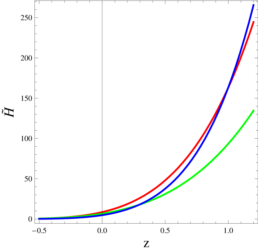
Figure 1: Plot of the reconstructed Hubble parameter $\tilde{H}$ obtained in Eq. (13).

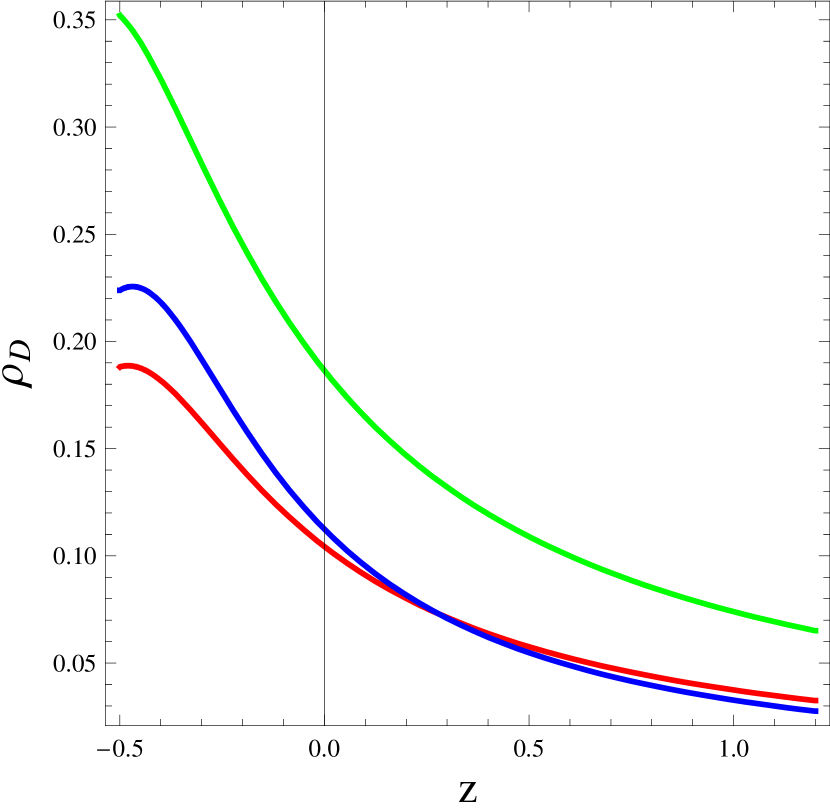
Figure 2: Plot of the reconstructed energy density $\rho_{D}$.
See Eq. (22)

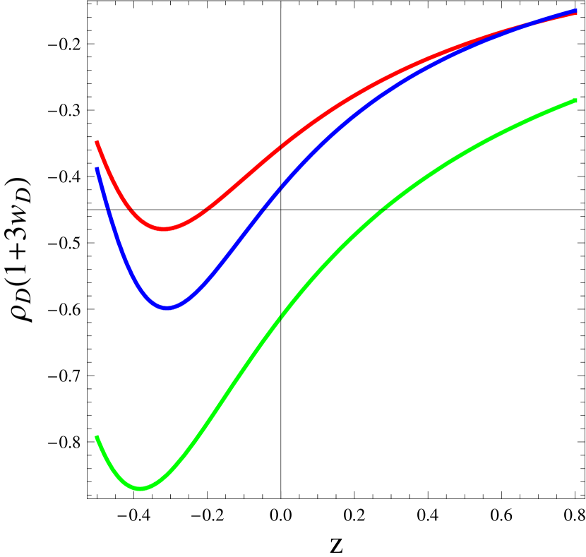
Figure 3: Plot of the evolution of $\rho_{D}(1+3w_{D})$ (strong energy condition test). See Eqs. (22) and (24).

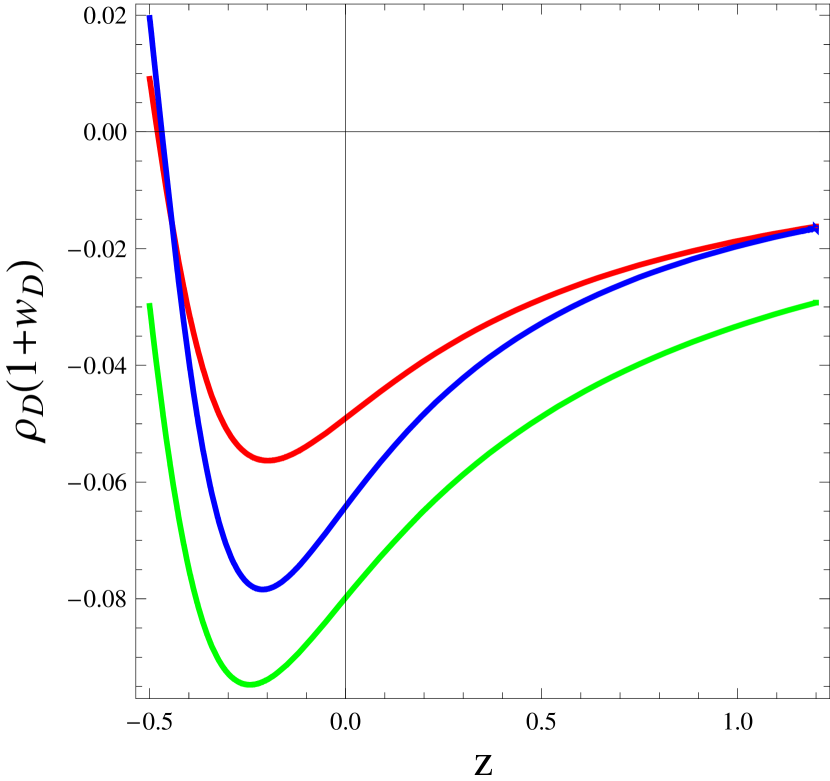
Figure 4: Plot of the evolution of $\rho_{D}(1+w_{D})$ (null energy condition test). See Eqs. (22) and (24).

We now plot the reconstructed cosmological parameters against the redshift $z$. In all Figures, we have that red, green and blue lines correspond to $\{\mu=0.65,~{}\nu=0.20\}$, $\{\mu=0.60,~{}\nu=0.25\}$ and $\{\mu=0.55,\nu=0.15\}$, respectively. For all other figures, the other parameters present in the equations we derived are set as $\alpha=5,~{}\beta=-0.7,~{}\gamma=-0.9,~{}\phi_{0}=0.12,~{}\omega=-\frac{3}{2}+10^{-22},~{}f_{0}=1,~{}V_{0}=2$. The choice of the value of the BD parameter $\omega$ is based on ref. Hrycyna . Observational results coming from SNeIa data suggest a range of possible values for the EoS parameter of $-1.67<w<-0.62$ MNR . Using a set of variations in the values of $\mu$ and $\nu$ in Eq. (24) we find that the results are in good agreement with MNR . In Table I, we are showing a set of values of the reconstructed EoS based on the chosen values of the parameters. It is apparent from this table that the EoS parameter $-1.67<w<-0.62$.

Table 1: Values of reconstructed $w_{D}$ (Eq. (24)) for different choices of parameter values.

Choice of $\alpha$, $\beta$ and $\gamma$	vales of $w_{D}~{}(\mu=0.55,~{}\nu=0.15)$	values of $w_{D}~{}(\mu=0.65,~{}\nu=0.20)$	values of $w_{D}~{}(\mu=0.60,~{}\nu=0.25)$
$(\alpha=5,~{}\beta=-0.7,~{}\gamma=-0.9)$	-1.47265	-1.47040	-1.47797
$(\alpha=4.5,~{}\beta=-0.6,~{}\gamma=-1)$	-1.57145	-1.56864	-1.57484
$(\alpha=4.1,~{}\beta=-0.8,~{}\gamma=-1.1)$	-1.25035	-1.24863	-1.25514

In Fig. 4, we observe the evolution of the reconstructed Hubble parameter $\tilde{H}$ with redshift $z=a^{-1}-1$. We observe a decaying pattern of $\tilde{H}$ with evolution of the universe. This in consistent with the accelerated expansion of the universe. In Fig. 4, the reconstructed NHDE density is plotted and indicates its dominance with the evolution of the universe. This is consistent with the current dark-energy dominated era.
We now want to have a deeper look into the Eq. (24) derived through the reconstructed $\tilde{H}$. In Eq. (24), the expression $3\left(s\left(a^{s}\eta_{5}\right)^{\eta_{2}}\nu-e^{a^{s}\eta_{5}}\left(2\mu-\nu\left(-s\eta_{4}+a^{s}s\eta_{6}+\alpha(2-\beta+\nu)\right)\right)\Gamma\left[\eta_{2},a^{s}\eta_{5}\right]\right)~{}\neq 0$. Considering the forms of $\eta_{X}~{}(X=1,2,..,6)$ it can be verified that the above expression is surely positive if $\alpha<0,~{}~{}-1<\nu<0$ or $\alpha>0,~{}~{}\nu<-1$. Since we have taken $\phi=\phi_{0}a^{\alpha}$, we have $\dot{\phi}=\alpha\phi H$. If $\alpha<0$, then the scalar field decays with the evolution of the universe.

Since the behavior of the remaining part of the expression is too complicated to make any inference on its “quintessence” or “phantom”-like behavior, we only depend on the strong and null energy conditions to put some light into the behavior of the equation of state parameter. Null energy condition is satisfied if $\rho_{D}(1+w_{D})\geq 0$ while the strong energy condition condition is satisfied if $\rho_{D}(1+w_{D})\geq 0~{}~{}\text{and}~{}~{}\rho_{D}(1+3w_{D})\geq 0$. Figs. 4 and 4 indicate that both of the energy conditions are violated. This indicates “phantom”-like behavior of the equation of state parameter.

In this Section, we reconstructed the NHDE in the framework of chameleon BD cosmology. In the following Section, our objective is to study the correspondence between this reconstructed NHDE model and the scalar field models, namely (i) Quintessence dark energy, (ii) DBI-essence dark energy and (iii) Tachyon dark energy.

II.1 Stability under a quantum correction

Following bamba5 ; bambaquantum we examine the stability for the obtained solutions of the crossing of the phantom divide under a quantum correction of massless conformally-invariant fields. Quantum effects produce the conformal anomaly bamba5 :

$$T_{A}=b\left(F+\frac{2}{3}\square R\right)+b^{\prime}G+b^{\prime\prime}\square R,$$ (25)

where

$$F = \frac{1}{3}R^{2}-2R_{ij}R^{ij}+R_{ijkl}R^{ijkl},$$ (26)

$$G = R^{2}-4R_{ij}R^{ij}+R_{ijkl}R^{ijkl}.$$ (27)

In the FRW universe, we have that:

$$F = 0,$$ (28)

$$G = 24(\dot{H}H^{2}+H^{4}).$$ (29)

For $N$ real scalar, $N_{1/2}$ Dirac spinor, $N_{1}$ vector fields, $N_{2}(=0~{}\textrm{or}~{}1)$ gravitons and $N_{HD}$ higher derivative conformal scalars, we have the following expressions for $b$ and $b^{\prime}$:

$$b = \frac{N+6N_{1/2}+12N_{1}+611N_{2}-8N_{HD}}{120(4\pi)^{2}},~{}~{}$$ (30)

$$b^{\prime} = -\frac{N+11N_{1/2}+62N_{1}+1411N_{2}-28N_{HD}}{360(4\pi)^{2}},$$ (31)

with $b^{\prime\prime}$ which can be arbitrary. If we assume that $T_{A}$ can be given by the effective energy density $\rho_{A}$ and pressure $p_{A}$ from the conformal anomaly as:

$$\dot{\rho}_{A}+3H(\rho_{A}+p_{A})=0,$$ (32)

the following expressions for $\rho_{A}$ and $p_{A}$ can be found:

$$\rho_{A} = -\frac{1}{a^{4}}\int dta^{4}HT_{A},$$ (33)

$$p_{A} = -\frac{1}{3a^{4}}\int dta^{4}HT_{A}+\frac{T_{A}}{3}.$$ (34)

At phantom crossing, we must have $\dot{H}=0$. If we assume that the magnitude of the Hubble rate $H$ could be the order of the present Hubble constant $H_{0}$, then for phantom crossing we have:

$$\rho_{D}=\frac{3\phi^{2}}{4\omega}\tilde{H}_{0}^{2}\mu$$ (35)

where $\tilde{H}_{0}^{2}=\tilde{H}^{2}|_{(a=1)}=\left(\frac{3}{8}\right)^{\eta_{4}}e^{-\eta_{6}}\eta_{1}\eta_{3}\left(-\eta_{5}\right)^{\eta_{4}}\Gamma\left[\eta_{2},\eta_{5}\right]$.

The results obtained in Eqs. (33) and (34) tell that we may assume $\rho_{A}\sim p_{A}\sim T_{A}$. Then, we find bambaquantum :

$$\rho_{A}\sim p_{A}\sim C\tilde{H}_{0}^{4}$$ (36)

where $C$ represents a dimensionless constant of the order of $\sim 10^{2\sim 3}$. Thus, for the reconstructed model, we obtain:

$$\frac{\rho_{D}}{\rho_{A}}=\frac{3\phi^{2}\mu}{4C\omega\tilde{H}_{0}^{2}}\approx 10^{19}\frac{\mu}{\tilde{H}_{0}^{2}},$$ (37)

hence we can conclude that

$$|\rho_{D}|\gg|\rho_{A}|.$$ (38)

Therefore, the quantum correction could be small when the phantom crossing occurs and the obtained solutions of the phantom crossing in this paper could be stable under the quantum correction.

III New holographic reconstruction of scalar field models in BD cosmology

Sahni and Starobinsky satro1 discussed various aspects of reconstructing the expansion history of the Universe and to probe the nature of dark energy. Below, we will study the correspondence between NHDE model and the quintessence, the DBI-essence and the tachyon scalar field models in the framework of flat chameleon Brans-Dicke universe. We will also reconstruct the potentials and the dynamics for these scalar field models. We can give the related results of scalar fields and potentials for the NHDE model in the flat chameleon Brans-Dicke universe. In order to establish this correspondence, we compare the energy density of the NHDE model given in Eq. (22) with the corresponding energy density of the scalar field model, and we also equate the EoS for these scalar models with the EoS for the NHDE model given in Eq. (24). We must also emphasize here that we indicate the scalar field with $\varphi$ in order to differ it from the scalar field $\phi$ in Brans-Dicke theory.

III.1 Reconstruction of quintessence dark energy model

Quintessence is a dynamical, evolving, spatially inhomogeneous component with negative pressure. Unlike a cosmological constant, the quintessential pressure and energy density evolve with the time and the EoS parameter may also do so. A common model of quintessence is the energy density associated with a scalar field $Q$ slowly rolling down a potential $V(Q)$. A detailed discussion on quintessence dark energy is available in the review quint0 . The energy density $\rho_{Q}$ and pressure $p_{Q}$ of the quintessence scalar field $\varphi$ are given, respectively, by quint1 ; quint2 ; quint3 :

$$\rho_{Q} = \frac{1}{2}\dot{\varphi}^{2}+V(\varphi),$$ (39)

$$p_{Q} = \frac{1}{2}\dot{\varphi}^{2}-V(\varphi).$$ (40)

Moreover, the EoS parameter can be written as follow:

$$w_{Q}=\frac{p_{Q}}{\rho_{Q}}=\frac{\dot{\varphi}^{2}-2V(\varphi)}{\dot{\varphi}^{2}+2V(\varphi)}.$$ (41)

As we are reconstructing the quintessence model based on NHDE in the framework of chameleon BD cosmology, we shall consider $\rho_{Q}=\rho_{D}$ and $w_{Q}=w_{D}$. Hence, we have:

$$\dot{\varphi}^{2} = \rho_{D}(1+w_{D}),$$ (42)

$$V(\varphi) = \frac{\rho_{D}}{2}(1-w_{D}),$$ (43)

where $\rho_{D}$ and $w_{D}$ are given in Eqs. (22) and (24), respectively. Based on the reconstructed Hubble parameter, we express $\dot{\varphi}^{2}$ and $V(\varphi)$ as functions of the scale factor $a$ as follow:

$$\dot{\varphi}(a)^{2} = -\frac{1}{\omega}3^{\eta_{4}}8^{-1-\eta_{4}}a^{\alpha(\beta-\nu)}e^{-a^{s}(\eta_{5}+\eta_{6})}\phi_{0}^{2}\eta_{1}\eta_{3}\left(-a^{s}\eta_{5}\right)^{\eta_{4}}\left(s\left(a^{s}\eta_{5}\right)^{\eta_{2}}\right.$$ (44)

$$\left.\left(-2\mu+\nu\left(-s\left(\eta_{2}+2\eta_{4}-a^{s}(\eta_{5}+2\eta_{6})\right)+\right.\right.\right.$$

$$\left.\left.\left.\alpha(2-2\beta+2\nu)\right)\right)+e^{a^{s}\eta_{5}}\left(\alpha^{2}\nu\left(\beta^{2}-2\beta(1+\nu)+\nu(2+\nu)\right)+s\left(s\eta_{4}^{2}\nu+2\eta_{4}\left(\mu-a^{s}s\eta_{6}\nu\right)+\right.\right.\right.$$

$$\left.\left.\left.a^{s}\eta_{6}\left(-2\mu+s\left(-1+a^{s}\eta_{6}\right)\nu\right)\right)+2\alpha\left(\beta\left(\mu+s\left(\eta_{4}-a^{s}\eta_{6}\right)\nu\right)-\nu\left(\mu+s\left(\eta_{4}-a^{s}\eta_{6}\right)(1+\nu)\right)\right)\right)\right.$$

$$\left.\times\Gamma\left[\eta_{2},a^{s}\eta_{5}\right]\right),$$

$$V(\varphi(a)) = -\frac{2^{-4-3\eta_{4}}3^{1+\eta_{4}}}{\omega}a^{\alpha(\beta-\nu)}e^{-a^{s}(\eta_{5}+\eta_{6})}\phi_{0}^{2}\eta_{1}\eta_{3}\left(-a^{s}\eta_{5}\right)^{\eta_{4}}\left(s\left(a^{s}\eta_{5}\right)^{\eta_{2}}\nu-\right.$$ (45)

$$\left.e^{a^{s}\eta_{5}}\left(2\mu-\nu\left(-s\eta_{4}+a^{s}s\eta_{6}+\alpha(2-\beta+\nu)\right)\right)\right.$$

$$\left.\Gamma\left[\eta_{2},a^{s}\eta_{5}\right]\right)\left(1-\left(s\left(a^{s}\eta_{5}\right)^{\eta_{2}}\left(-2\mu+\nu\left(-3-s\left(\eta_{2}+2\eta_{4}-a^{s}(\eta_{5}+2\eta_{6})\right)+2\alpha(1-\beta+\nu)\right)\right)+\right.\right.$$

$$\left.\left.e^{a^{s}\eta_{5}}\left(a^{2s}s^{2}\eta_{6}^{2}\nu+(3+s\eta_{4}+\alpha(\beta-\nu))(2\mu+(s\eta_{4}+\alpha(-2+\beta-\nu))\nu)-\right.\right.\right.$$

$$\left.\left.\left.a^{s}s\eta_{6}(2\mu+(3+s+2s\eta_{4}+2\alpha(-1+\beta-\nu))\nu)\right)\Gamma\left[\eta_{2},a^{s}\eta_{5}\right]\right)\right.$$

$$\left./\left(3\left(s\left(a^{s}\eta_{5}\right)^{\eta_{2}}\nu-e^{a^{s}\eta_{5}}\left(2\mu-\nu\left(-s\eta_{4}+a^{s}s\eta_{6}+\alpha(2-\beta+\nu)\right)\right)\Gamma\left[\eta_{2},a^{s}\eta_{5}\right]\right)\right)\right).$$

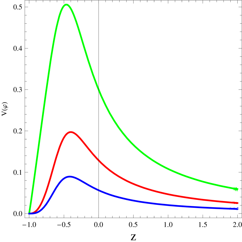
Figure 5: Plot of the evolution of the reconstructed potential $V(\varphi)$ for the reconstructed quintessence dark energy model. See Eq. (45).

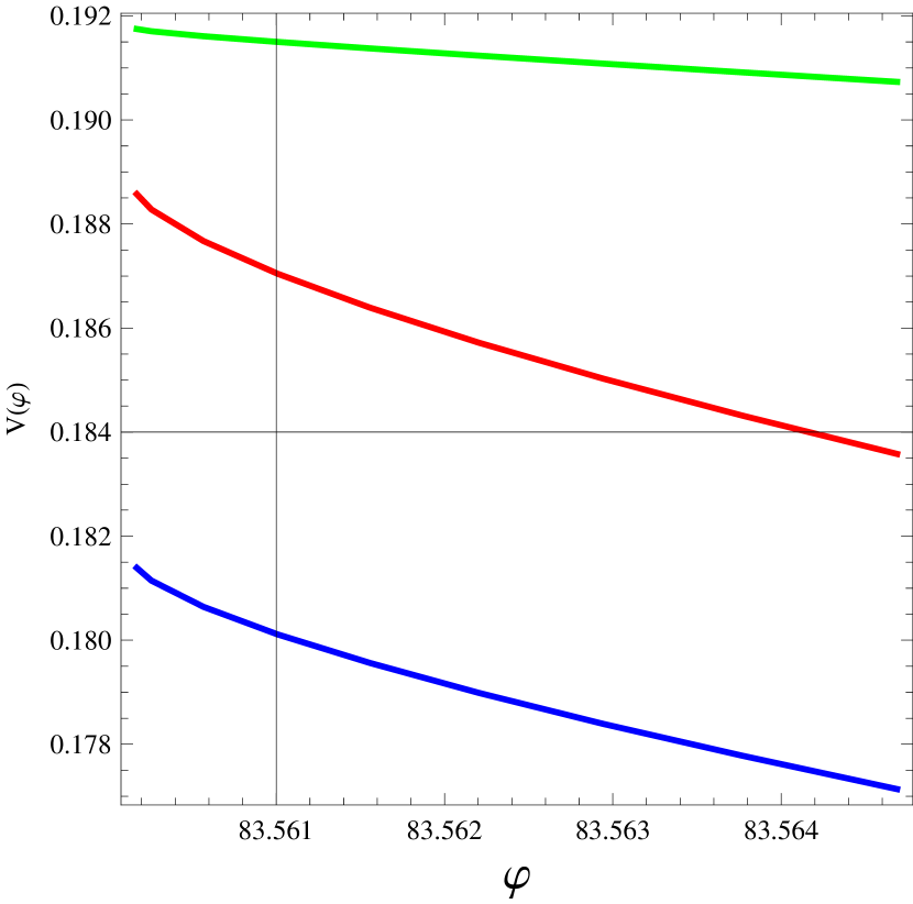
Figure 6: Plot of the evolution of the reconstructed potential $V(\varphi)$ (Eq. (45)) with reconstructed scalar field $\varphi$ (Eq. (44)) of the quintessence dark energy model.

III.2 Reconstruction of DBI-essence dark energy model

During the last few years, there have been many works aiming at connecting string theory with inflation which is also a phase of accelerated expansion. Martin and Yamaguchi martin introduced a scalar-field model of dark energy with a non-standard Dirac-Born-Infeld (DBI) kinetic term. This model is dubbed as “DBI-essence dark energy” and the energy density $\rho_{DBI}$ and the pressure $p_{DBI}$ of the DBI-essence model are given, respectively, by martin :

$$\rho_{DBI} = (\eta-1)T(\varphi)+V(\varphi),~{}~{}~{}~{}~{}~{}~{}~{}~{}~{}~{}~{}~{}~{}~{}~{}~{}~{}$$ (46)

$$p_{DBI} = \left(\frac{\eta-1}{\eta}\right)T(\varphi)-V(\varphi),~{}~{}~{}~{}~{}~{}~{}~{}~{}~{}~{}~{}~{}~{}~{}~{}~{}~{}$$ (47)

where:

$$\eta=\frac{1}{\sqrt{1-\frac{\dot{\varphi}^{2}}{T}}}.$$ (48)

The EoS parameter for the DBI-essence scalar field model can be written as follow:

$$w_{DBI}=\frac{p_{DBI}}{\rho_{DBI}}=\frac{\left(\eta-1\right)T(\varphi)-V(\varphi)\eta}{\eta\left((\eta-1)T(\varphi)+V(\varphi)\right)}.$$ (49)

In the present work, we shall assume that $T=n\dot{\varphi}^{2}$, where $n>0$. Since we are considering a correspondence between DBI-essence dark energy and the reconstructed NHDE model, we consider $\rho_{DBI}=\rho_{D}$ and $w_{DBI}=w_{D}$. The based on Eq. (13) we get the reconstructed scalar field $\varphi$ as function of the scale factor $a$ as follow:

$$\dot{\varphi}(a)^{2} = -\frac{3^{\eta_{4}}8^{-1-\eta_{4}}a^{\alpha(\beta-\nu)}}{\omega}\times$$ (50)

$$e^{-a^{s}(\eta_{5}+\eta_{6})}\sqrt{1-\frac{1}{n}}\phi_{0}^{2}\eta_{1}\eta_{3}\left(-a^{s}\eta_{5}\right)^{\eta_{4}}\left(s\left(a^{s}\eta_{5}\right)^{\eta_{2}}\left(-2\mu+\nu\left(-s\left(\eta_{2}+2\eta_{4}-a^{s}(\eta_{5}+2\eta_{6})\right)+\right.\right.\right.$$

$$\left.\left.\left.\alpha(2-2\beta+2\nu)\right)\right)+e^{a^{s}\eta_{5}}\left(\alpha^{2}\nu\left(\beta^{2}-2\beta(1+\nu)+\nu(2+\nu)\right)+s\left(s\eta_{4}^{2}\nu+2\eta_{4}\left(\mu-a^{s}s\eta_{6}\nu\right)+\right.\right.\right.$$

$$\left.\left.\left.a^{s}\eta_{6}\left(-2\mu+s\left(-1+a^{s}\eta_{6}\right)\nu\right)\right)+\right.\right.$$

$$\left.\left.2\alpha\left(\beta\left(\mu+s\left(\eta_{4}-a^{s}\eta_{6}\right)\nu\right)-\nu\left(\mu+s\left(\eta_{4}-a^{s}\eta_{6}\right)(1+\nu)\right)\right)\right)\Gamma\left[\eta_{2},a^{s}\eta_{5}\right]\right),$$

$$V(\varphi(a)) = \frac{3^{\eta_{4}}8^{-1-\eta_{4}}}{\omega}a^{\alpha(\beta-\nu)}e^{-a^{s}(\eta_{5}+\eta_{6})}\phi_{0}^{2}\eta_{1}\eta_{3}\left(-a^{s}\eta_{5}\right)^{\eta_{4}}\times$$ (51)

$$\left(-3\left(s\left(a^{s}\eta_{5}\right)^{\eta_{2}}\nu-e^{a^{s}\eta_{5}}\left(2\mu-\nu\left(-s\eta_{4}+a^{s}s\eta_{6}+\alpha(2-\beta+\nu)\right)\right)\Gamma\left[\eta_{2},a^{s}\eta_{5}\right]\right)+\right.$$

$$\left.\left(-1+\sqrt{\frac{n}{n-1}}\right)\sqrt{\frac{n-1}{n}}n\left(s\left(a^{s}\eta_{5}\right)^{\eta_{2}}\left(-2\mu+\nu\left(-s\left(\eta_{2}+2\eta_{4}-a^{s}(\eta_{5}+2\eta_{6})\right)+\right.\right.\right.\right.$$

$$\left.\left.\left.\left.\alpha(2-2\beta+2\nu)\right)\right)+e^{a^{s}\eta_{5}}\left(\alpha^{2}\nu\left(\beta^{2}-2\beta(1+\nu)+\nu(2+\nu)\right)+s\left(s\eta_{4}^{2}\nu+2\eta_{4}\left(\mu-a^{s}s\eta_{6}\nu\right)+\right.\right.\right.\right.$$

$$\left.\left.\left.\left.a^{s}\eta_{6}\left(-2\mu+s\left(-1+a^{s}\eta_{6}\right)\nu\right)\right)+2\alpha\left(\beta\left(\mu+s\left(\eta_{4}-a^{s}\eta_{6}\right)\nu\right)\right.\right.\right.\right.$$

$$\left.\left.\left.\left.-\nu\left(\mu+s\left(\eta_{4}-a^{s}\eta_{6}\right)(1+\nu)\right)\right)\right)\Gamma\left[\eta_{2},a^{s}\eta_{5}\right]\right)\right).$$

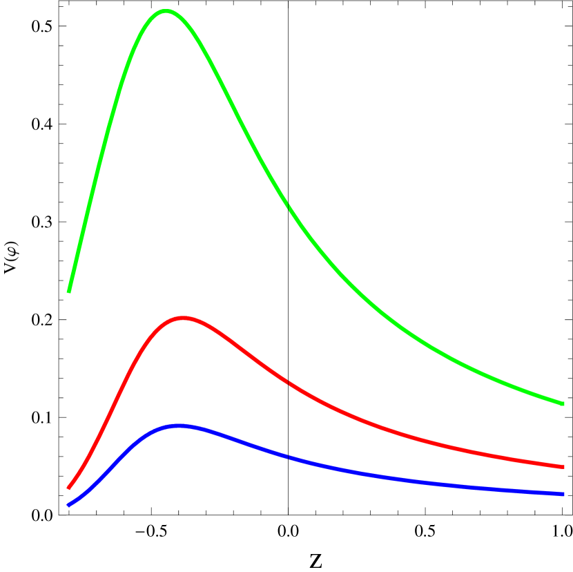
Figure 7: Plot of the evolution of the reconstructed potential $V(\varphi)$ for the reconstructed DBI-essence dark energy model. See Eq. (51). We have chosen $n=1.5$.

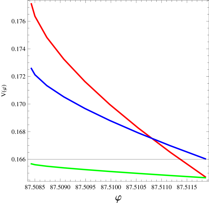
Figure 8: Plot of the evolution of the reconstructed potential $V(\varphi)$ (Eq. (51)) with reconstructed scalar field $\varphi$ (Eq. (50)) of the DBI-essence dark energy model.We have chosen $n=1.5$.

III.3 Reconstruction of tachyon dark energy model

Tachyonic condensate in a class of string theories can be described by an effective scalar field with a Lagrangian of the form $L=-V(\phi)(1-\partial_{a}\phi\partial^{a}\phi)^{1/2}$. Since this Lagrangian has also a potential function $V(\phi)$, any form of cosmological evolution (that is, any $a(t)$) can be obtained with the tachyonic field as the source by choosing $V(\phi)$ suitably paddy1 . Cosmological effects of homogeneous tachyon matter coexisting with non-relativistic matter and radiation have been studied by paddy2 . The energy density $\rho_{T}$ and the pressure $p_{T}$ of the tachyon scalar field model are given, respectively, by paddy1 :

$$\rho_{T} = \frac{V(\varphi)}{\sqrt{1-\dot{\varphi}^{2}}},$$ (52)

$$p_{T} = -V(\varphi)\sqrt{1-\dot{\varphi}^{2}},$$ (53)

while the EoS parameter can be written as follow:

$$w_{T}=\frac{p_{T}}{\rho_{T}}=\dot{\varphi}^{2}-1.$$ (54)

For the correspondence under consideration, we have $\rho_{T}=\rho_{D}$ and $w_{D}=w_{T}$. Using the same procedure used before, we reconstruct the scalar field $\varphi$ and the potential $V(\varphi)$ as follow:

$$\dot{\varphi}(a)^{2} = 1+\left(s\left(a^{s}\eta_{5}\right)^{\eta_{2}}\left(-2\mu+\nu\left(-3-s\left(\eta_{2}+2\eta_{4}-a^{s}(\eta_{5}+2\eta_{6})\right)+\right.\right.\right.$$ (55)

$$\left.\left.\left.2\alpha(1-\beta+\nu)\right)\right)+e^{a^{s}\eta_{5}}\left(a^{2s}s^{2}\eta_{6}^{2}\nu+(3+s\eta_{4}+\alpha(\beta-\nu))\times\right.\right.$$

$$\left.\left.(2\mu+(s\eta_{4}+\alpha(-2+\beta-\nu))\nu)-a^{s}s\eta_{6}(2\mu+(3+s+2s\eta_{4}+2\alpha(-1+\beta-\nu))\nu)\right)\Gamma\left[\eta_{2},a^{s}\eta_{5}\right]\right)\times$$

$$\left(3\left(s\left(a^{s}\eta_{5}\right)^{\eta_{2}}\nu-e^{a^{s}\eta_{5}}\left(2\mu-\nu\left(-s\eta_{4}+a^{s}s\eta_{6}+\alpha(2-\beta+\nu)\right)\right)\Gamma\left[\eta_{2},a^{s}\eta_{5}\right]\right)\right)^{-1},$$

$$V(\varphi(a)) = \left[-\frac{3^{1+2\eta_{4}}a^{2\alpha(\beta-\nu)}e^{-2a^{s}(\eta_{5}+\eta_{6})}\phi_{0}^{4}\eta_{1}^{2}\eta_{3}^{2}}{\omega^{2}}\times 2^{-6(1+\eta_{4})}\right.$$ (56)

$$\left.\left(-a^{s}\eta_{5}\right)^{2\eta_{4}}\left(s\left(a^{s}\eta_{5}\right)^{\eta_{2}}\left(-2\mu+\nu\left(-3-s\left(\eta_{2}+2\eta_{4}-a^{s}(\eta_{5}+2\eta_{6})\right)+2\alpha(1-\beta+\nu)\right)\right)+\right.\right.$$

$$\left.\left.e^{a^{s}\eta_{5}}\left(a^{2s}s^{2}\eta_{6}^{2}\nu+(3+s\eta_{4}+\alpha(\beta-\nu))(2\mu+(s\eta_{4}+\alpha(-2+\beta-\nu))\nu)-\right.\right.\right.$$

$$\left.\left.\left.a^{s}s\eta_{6}(2\mu+(3+s+2s\eta_{4}+2\alpha(-1+\beta-\nu))\nu)\right)\Gamma\times\right.\right.$$

$$\left.\left.\left[\eta_{2},a^{s}\eta_{5}\right]\right)\left(s\left(a^{s}\eta_{5}\right)^{\eta_{2}}\nu-e^{a^{s}\eta_{5}}\left(2\mu-\nu\left(-s\eta_{4}+a^{s}s\eta_{6}+\right.\right.\right.\right.$$

$$\left.\left.\left.\left.\alpha(2-\beta+\nu)\right)\right)\Gamma\left[\eta_{2},a^{s}\eta_{5}\right]\right)\right]^{1/2}$$

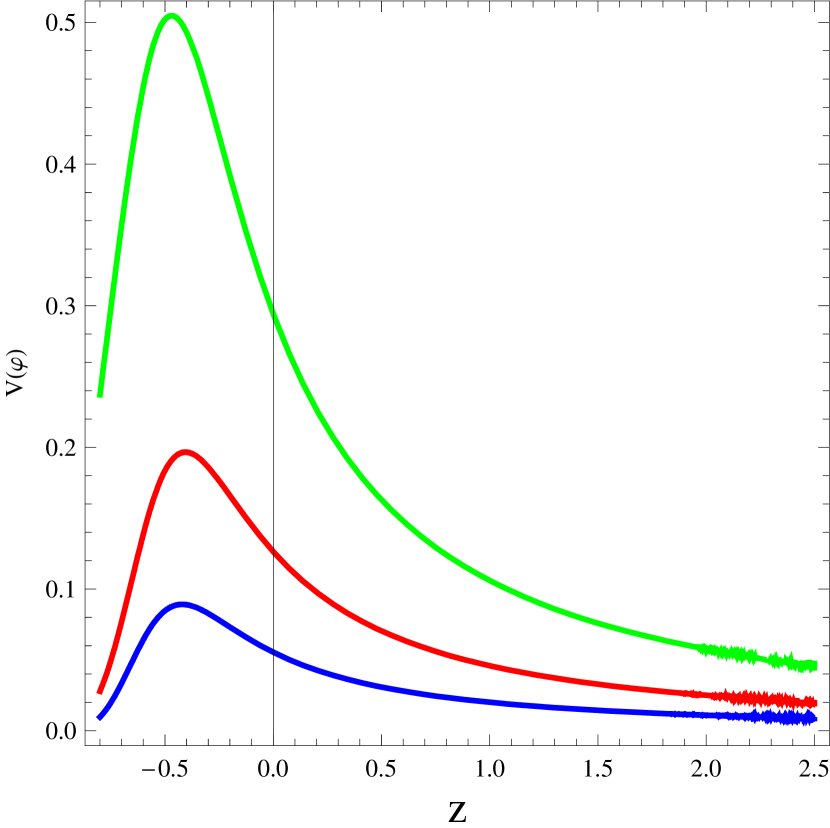
Figure 9: Plot of the evolution of the reconstructed potential $V(\varphi)$ for the reconstructed tachyon dark energy model. See Eq. (56).

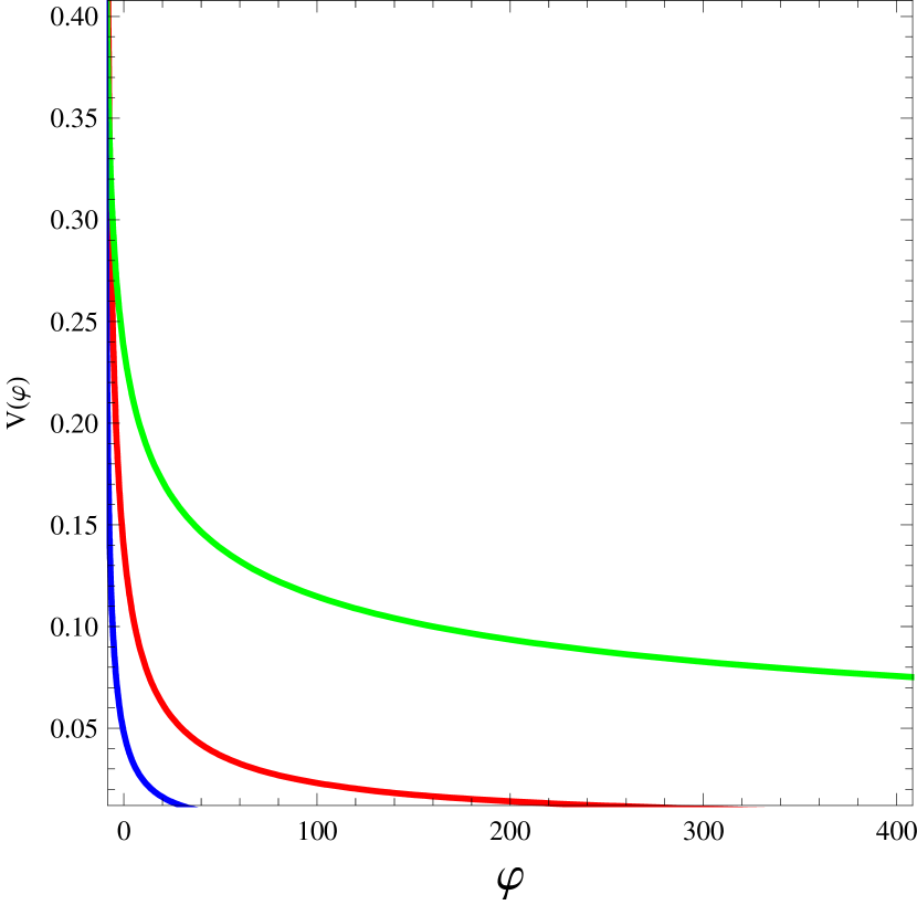
Figure 10: Plot of the evolution of the reconstructed potential $V(\varphi)$ (Eq. (56)) with reconstructed scalar field $\varphi$ (Eq. (55)) of the tachyon dark energy model.

III.4 Discussion

In this paper, we studied the main cosmological properties of the New Holographic Dark Energy (HNDE) model in the framework of Brans-Dicke chameleon cosmology. We considered a particular ansatz for the parameters $\phi$, $V$ and $f$ in which their expressions are given in the power law form. We decided to consider different aspects to study. First of all, we reconstructed the expression of the Hubble parameter $H$ and, accordingly, the expression of the density $\rho_{D}$ of the NHDE in the context of chameleon Brans-Dicke chameleon cosmology. We also tested the Weak Energy condition (WEC) and the Strong Energy Condition (SEC) for the reconstructed model we obtained. Considering three cases, namely $\{\mu=0.65,~{}\nu=0.20\}$, $\{\mu=0.60,~{}\nu=0.25\}$ and $\{\mu=0.55,\nu=0.15\}$ setting the other parameters as $\alpha=5,~{}\beta=-0.7,~{}\gamma=-0.9,~{}\phi_{0}=0.12,~{}\omega=-\frac{3}{2}+10^{-22},~{}f_{0}=1,~{}V_{0}=2$ and BD parameter $\omega$ following Hrycyna we have computed the reconstructed EoS parameter. Observational results coming from SNeIa data suggest a limit of the EoS parameter as $-1.67<w<-0.62$ MNR . Using a set values of $\mu$ and $\nu$ in Eq. (24) we found that the results are in good agreement with observations of MNR . Finally, we reconstructed three scalar field models of dark energy (namely, the quintessence, the DBI-essence and the tachyon ones) based on the NHDE model in the framework of BD cosmology. For the three scalar field models we considered, we have reconstructed the corresponding potentials and scalar fields. To further elucidate our reconstructions, we have plotted the reconstructed potential $V(\varphi)$ against $z$ and made parametric plots between $\varphi$ and $V({\varphi})$ in Figs. 6, 6, 8, 8, 10 and 10. It is apparent from the plots that the potential $V(\varphi)$ is increasing up to redshifts of the order of $z\approx-0.5$, afterwards it starts to decay. In the plots of $\varphi-V(\varphi)$, it appears that the potential has a decreasing behavior with the scalar field $\varphi$.

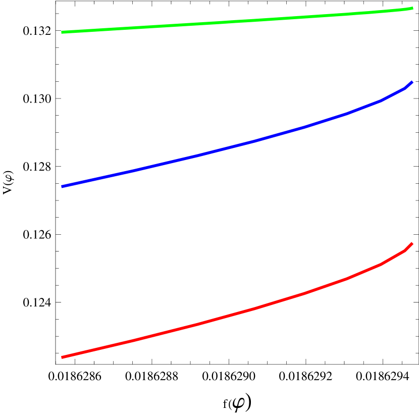
Figure 11: Plot of the evolution of the reconstructed potential $V(\varphi)$ with $f(\varphi)$ for quintessence dark energy model.

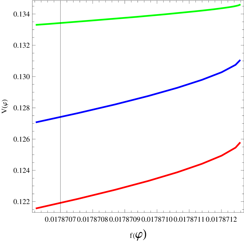
Figure 12: Plot of the evolution of the reconstructed potential $V(\varphi)$ with $f(\varphi)$ for DBI-essence dark energy model.

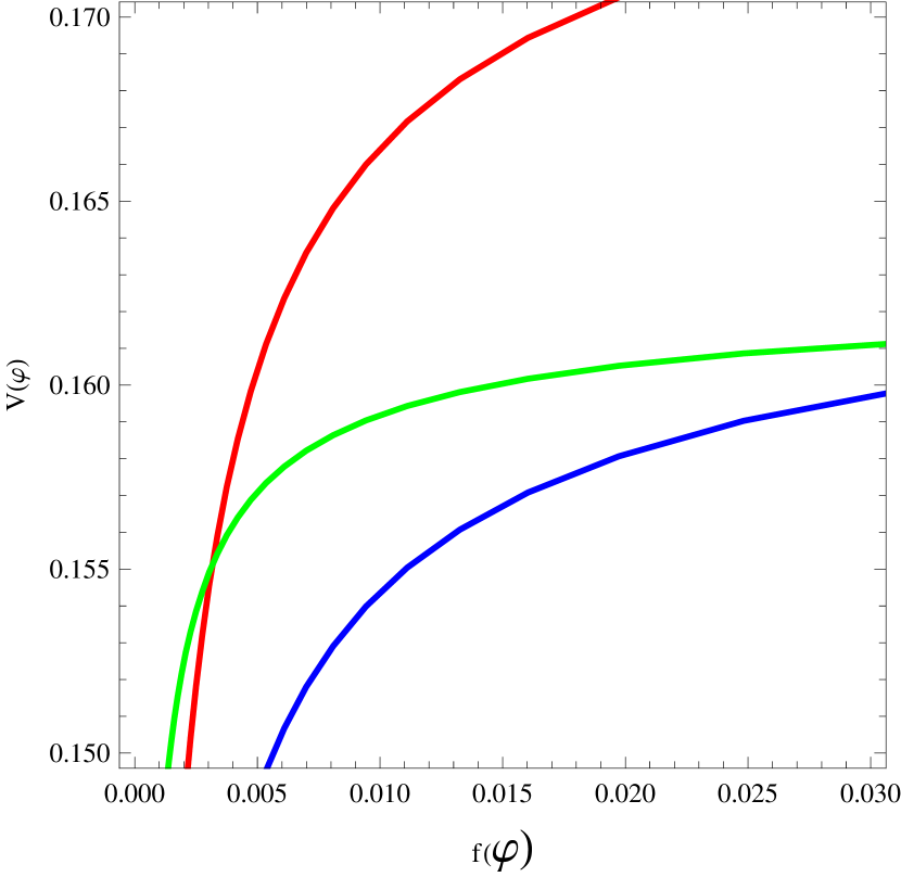
Figure 13: Plot of the evolution of the reconstructed potential $V(\varphi)$ with $f(\varphi)$ for tachyon dark energy model.

In order to have a look into the behavior of the reconstructed potential against coupling function $f$ we discuss the Figs. 13, 13 and 13, where we observe that the reconstructed potentials are increasing with $f$. This indicates that the potential increasing as the matter-chameleon coupling is getting stronger. It is further noted that the rate of increase in the potential is much higher in the case of tachyon than the cases of quintessence and DBI.

IV Concluding remarks

In the present work we have used a reconstruction scheme for new holographic dark energy model with energy density given by $\rho_{D}=\frac{3\phi^{2}}{4\omega}\left(\mu H^{2}+\nu\dot{H}\right)$ in the framework of Brans-Dicke cosmology taking the ansatz $\phi=\phi_{0}a^{\alpha},~{}~{}V=V_{0}\phi^{\beta},~{}~{}f=f_{0}\phi^{\gamma}$. Outcomes of the study are:

• Considering $\rho=\rho_{D}$ in the first modified field equation of BD theory leads to a linear differential equation which could be solved analytically to have a solution for the reconstructed Hubble parameter in terms of scale factor $a$; when plotted against redshift $z=a^{-1}-1$, it exhibited decaying pattern with the evolution of the universe (i.e., decreases in $z$) and this is consistent with the accelerated expansion of the universe.

• The NHDE energy density, as reconstructed through Hubble parameter, when plotted against $z$, is found to increase with evolution of the universe and it is consistent with the evolution of the universe from matter to dark energy domination.

• Violation of strong energy condition, as expected in the framework of Einstein gravity, has also been found for the reconstructed NHDE model in the framework of BD gravity.

• The reconstructed equation of state (EoS) parameter has been found to exhibit “phantom”-like behavior, i.e. $w_{D}<-1$.

• Considering three different combinations of the parameters $\mu$ and $\nu$, namely $\{\mu=0.65,~{}\nu=0.20\}$, $\{\mu=0.60,~{}\nu=0.25\}$ and $\{\mu=0.55,\nu=0.15\}$ and setting the other parameters as $\alpha=5,~{}\beta=-0.7,~{}\gamma=-0.9,~{}\phi_{0}=0.12,~{}\omega=-\frac{3}{2}+10^{-22},~{}f_{0}=1,~{}V_{0}=2$ and the BD parameter $\omega$ following Hrycyna , we have computed the reconstructed EoS parameter for the reconstructed NHDE. Observational results coming from SNeIa data suggest a limit of the EoS parameter as $-1.67<w<-0.62$ MNR . Using a set of variations in the values of $\mu$ and $\nu$ in Eq. (24) we found that the results are in good agreement with observations of MNR (see Table I).

In the following phase of the study, we considered the correspondence between the reconstructed new holographic dark energy in the framework of BD gravity and some scalar field dark energy models in a manner under which the two scenarios can be simultaneously valid. This type of approach is available in cosmological literature (e.g., motiv1 ; motiv2 ; motiv3 ). We have constructed the potentials and the scalar fields of these models. We observed that $\frac{dV}{dz}>0$ for all of the reconstructed scalar field models upt o $z\approx-0.5$ and, at very late stage, (i.e., $z<-0.5$), we have $\frac{dV}{dz}<0$. Moreover, $\frac{dV}{d\phi}<0$ for all of the models.

In summary, by generalizing the previous works motiv1 ; motiv2 ; motiv3 to the NHDE model with $\rho_{D}=\frac{3\phi^{2}}{4\omega}(\mu H^{2}+\nu\dot{H})$ in the framework of chameleon Brans-Dicke cosmology, we have obtained the evolution of EoS. Following motiv1 ; bisbar we have considered $V$, $\phi$ and $f$ in power-law form and accordingly reconstructed Hubble parameter. This approach differs from motiv1 in the sense that instead of considering Brans-Dicke cosmology, we have considered chameleon Brans-Dicke with coupling function $f$. We have tested SEC and WEC conditions and interpreted evolution of EoS from them. With some choice of the model parameters we computed EoS and found the the computed values of EoS are consistent with the observational results coming from SNeIa data that suggest a limit of the EoS parameter as $-1.67<w<-0.62$ MNR . Subsequently we examined the stability for the obtained solutions of the crossing of the phantom divide under a quantum correction of massless conformally-invariant fields and we have seen that quantum correction could be small when the phantom crossing occurs and the obtained solutions of the phantom crossing could be stable under the quantum correction. In the subsequent phase, we have established a correspondence between the NHDE model and the quintessence, the DBI-essence and the tachyon scalar field models in the framework of chameleon Brans-Dicke cosmology. We reconstruct the potentials and the dynamics for these three scalar field models we have considered. The reconstructed potentials are found to increase with evolution of the universe and in a very late stage they are observed to decay. It is also observed through $f(\varphi)-V(\varphi)$ plot that the potential is increasing with $f$, which indicates that the potential increases as the matter-chameleon coupling gets stronger with evolution of the universe.

V Acknowledgements

Sincere thanks are due to the anonymous reviewer for constructive suggestions. Project Grant of DST, Govt. of India no. SR/FTP/PS-167/2011 is duly acknowledged by the first author. Also, the first authors acknowledges the facilities provided by IUCAA, Pune, India, where a major portion of the work was carried out during a scientific visit in December, 2013-January, 2014.

References

- (1) A. G. Riess et al., Astron. J. 116, 1009 (1998) [doi: 10.1086/300499].
- (2) S. Perlmutter, Astrophys. J. 517, 565 (1999) [doi: 10.1086/307221].
- (3) R. A. Knop et al., Astrophys. J. 598, 102 (2003) [doi: 10.1086/378560].
- (4) D. N. Spergel et al., Astrophys. J. Suppl. 148, 175 (2003) [doi: 10.1086/377226].
- (5) E. Komatsu et al., Astrophys. J. Suppl. 192, 18 (2011)[doi: 10.1088/0067-0049/192/2/18].
- (6) Planck Collaboration, Ade, P. A. R., Aghanim, N., et al. 2013, arXiv:1303.5076.
- (7) D. J. Eisenstein et al. [SDSS Collaboration], Astrophys. J. 633, 560 (2005) [doi: 10.1086/466512].
- (8) W. J. Percival et al., Mon. Not. Roy. Astron. Soc. 401, 2148 (2010) [doi: 10.1111/j.1365-2966.2009.15812.x].
- (9) E. J. Copeland, M. Sami, S. Tsujikawa, Int. J. Mod. Phys. D, 15, 1753 (2006) [doi: 10.1142/S021827180600942X].
- (10) K. Bamba, S. Capozziello, S. Nojiri, S. D. Odintsov, Astrophys. Space Sci., 342, 155 (2012) [doi: 10.1007/s10509-012-1181-8].
- (11) R. R. Caldwell, M. Kamionkowski, Ann. Rev. Nucl. Part. Sci. 59, 397 (2009) [doi: 10.1146/annurev-nucl-010709-151330].
- (12) S. Nojiri, S. D. Odintsov, Phys. Rep., 505, 59 (2011) [doi: 10.1016/j.physrep.2011.04.001].
- (13) T. Clifton, P. G. Ferreira, A. Padilla, C. Skordis, Phys. Rept. 513, 1 (2012) [doi: 10.1016/j.physrep.2012.01.001].
- (14) S. Capozziello, M. De Laurentis, S. D. Odintsov, Eur. Phys. J. C 72, 2068 (2012) [doi: 10.1140/epjc/s10052-012-2068-0].
- (15) S. Tsujikawa, Lect. Notes Phys. 800, 99 (2010) [doi: 10.1007/978-3-642-10598-2_3].
- (16) V. Sahni, A. A. Starobinsky, Int. J. Mod. Phys. D 9, 373 (2000) [doi: 10.1142/S0218271800000542].
- (17) V. Sahni, A. A. Starobinsky, Int. J. Mod. Phys. D 15, 2105 (2006) [doi: 10.1142/S0218271806009704].
- (18) H. Motohashi, A. A. Starobinsky, J. Yokoyama, Prog. Theor. Phys. 123 , 887 (2010) [doi: 10.1143/PTP.124.541].
- (19) P. J. E. Peebles, B. Ratra, Rev. Mod. Phys. 75, 559 (2003) [doi: 10.1103/RevModPhys.75.559].
- (20) A. Shafieloo, V. Sahni, A. A. Starobinsky, Phys. Rev. D 80, 101301 (2009) [doi: 10.1103/PhysRevD.80.101301].
- (21) A. A. Starobinsky, Phys. Lett. B 91, 99 (1980) [doi: 10.1016/0370-2693(80)90670-X].
- (22) S. Nojiri, S. D. Odintsov, O. G. Gorbunova, J. Phys. A: Math. Gen. 39, 6627 (2006) [doi: 10.1088/0305-4470/39/21/S62].
- (23) A. V. Astashenok, S. Nojiri, S. D. Odintsov, R. J. Scherrer, Phys. Lett. B 713, 145 (2012) [doi: 10.1016/j.physletb.2012.06.017].
- (24) B. Gumjudpai, T. Naskar, M. Sami, S. Tsujikawa, J. Cosmol. Astropart. Phys. 06, 007 (2005) [doi: 10.1088/1475-7516/2005/06/007].
- (25) E. Elizalde, S. Nojiri, S. D. Odintsov, Phys. Rev. D 70, 043539 (2004) [doi: 10.1103/PhysRevD.70.043539].
- (26) S. Nojiri, S. D. Odintsov, S. Tsujikawa, Phys. Rev. D 71, 063004 (2005) [doi: 10.1103/PhysRevD.71.063004].
- (27) H. Zhang, Z-H. Zhu, Phys. Rev. D 73, 043518 (2006) [doi: 10.1103/PhysRevD.73.043518].
- (28) K. Bamba, J. Matsumoto, S. Nojiri, Phys. Rev. D 85, 084026 (2012) [doi: 10.1103/PhysRevD.85.084026].
- (29) M. Forte, Phys. Rev. D 90, 027302 (2014) [doi: 10.1103/PhysRevD.90.027302].
- (30) M. Li, Phys. Lett. B, 603, 1 (2004) [doi: 10.1016/j.physletb.2004.10.014].
- (31) E. Elizalde, S. Nojiri, S. D. Odintsov, P. Wang, Phys. Rev. D 71, 103504 (2005) [doi: 10.1103/PhysRevD.71.103504].
- (32) S. Nojiri, S. D. Odintsov, Gen. Rel. Grav. 38, 1285 (2006)[doi: 10.1007/s10714-006-0301-6].
- (33) S. del Campo, J. C. Fabris, R. Herrera, W. Zimdahl, Phys. Rev. D 83, 123006 (2011) [doi: 10.1103/PhysRevD.83.123006].
- (34) J-L. Cui, J-F. Zhang, Eur. Phys. J. C 74, 2849 (2014) [doi: 10.1140/epjc/s10052-014-2849-8].
- (35) Q-G. Huang, Y. Gong, JCAP 0408, 006 (2004) [doi: 10.1088/1475-7516/2004/08/006].
- (36) Q-G. Huang, M. Li, JCAP 0503, 001 (2005) [doi: 10.1088/1475-7516/2005/03/001].
- (37) X. Zhang, F-Q. Wu, Phys. Rev. D 76, 023502 (2007) [doi: 10.1103/PhysRevD.76.023502].
- (38) Y-F. Cai, E. N. Saridakis, M. R. Setare, J-Q. Xia, Phys. Rep. 493, 1 (2010) [doi: 10.1016/j.physrep.2010.04.001].
- (39) S. Nojiri, S. D. Odintsov, S. Tsujikawa, Phys. Rev. D 71, 063004 (2005) [doi: 10.1103/PhysRevD.71.063004].
- (40) A. A. Starobinsky, Phys. Rev. Lett. 85, 2236 (2000)[doi: 10.1103/PhysRevLett.85.2236].
- (41) S. Nojiri and S. D. Odintsov, Phys. Lett. B 562, 147 (2003) [doi: 10.1016/S0370-2693(03)00594-X]
- (42) S. Nojiri and S. D. Odintsov, Phys. Lett. B 571, 1 (2003) [doi: 10.1016/j.physletb.2003.08.013]
- (43) S. Nojiri and S. D. Odintsov, Phys. Lett. B 565, 1 (2003) [doi: 10.1016/S0370-2693(03)00753-6]
- (44) I. Brevik, S. Nojiri,S. D. Odintsov and L. Vanzo, Phys. Rev. D 70, 043520 (2004) [doi: 10.1103/PhysRevD.70.043520]
- (45) S. Nojiri, S. D. Odintsov, Proc. Sci. WC 2004, 024 (2004) [arXiv:hep-th/0412030].
- (46) B. Novosyadlyj, O. Sergijenko, R. Durrer, V. Pelykh, JCAP (2013) [doi: 10.1088/1475-7516/2013/06/042].
- (47) M. R. Setare and E. N. Saridakis, Phys. Rev. D 79, 043005 (2009) [doi: 10.1103/PhysRevD.79.043005].
- (48) H. Wei, R-G. Cai, D-F. Zeng, Class. Quantum Grav. 22, 3189 (2005) [doi: 10.1088/0264-9381/22/16/005].
- (49) M. Sharif, A. Jawad, Eur. Phys. J. C 72, 2097 (2012) [doi: 10.1140/epjc/s10052-012-2097-8].
- (50) A. Jawad, S. Chattopadhyay, A. Pasqua, Astrophys. Space Sci. 346, 273 (2013)[doi: 10.1007/s10509-014-2010-z].
- (51) M. Malekjani, A. Khodam-Mohammadi, N. Nazari-pooya, Astrophys. Space Sci. 332, 515 (2011) [doi: 10.1007/s10509-010-0550-4].
- (52) U. Debnath, S. Chattopadhyay, Int. J. Theor. Phys. 52, 1250 (2013) [doi: 10.1007/s10773-012-1440-z].
- (53) S. Nojiri, S. D. Odintsov, Phys. Lett. B 716, 377 (2012) [doi: 10.1016/j.physletb.2012.08.049].
- (54) S. Nojiri, S. D. Odintsov, N. Shirai, J. Cosmol. Astropart. Phys. 1305, 020 (2013) [doi: 10.1088/1475-7516/2013/05/020].
- (55) K. Bamba, S. Nojiri, S. D. Odintsov, Report OCHA-PP-323 (2014) [arXiv:1406.2417 [hep-th]].
- (56) W. Yang, Y. Wu, L. Song, Y. Su, J. Li, D. Zhang, X. Wang, Mod. Phys. Lett. A 26, 191 (2011) [doi: 10.1142/S0217732311034682]
- (57) K. Karami, J. Fehri, Phys. Lett. B 684, 61 (2010) [doi: 10.1016/j.physletb.2009.12.060].
- (58) A. Sheykhi, Phys. Lett. B 681, 205 (2009) [doi: 10.1016/j.physletb.2009.10.011].
- (59) L. N. Granda, A. Oliveros, Phys. Lett. B 669, 275 (2008) [doi: 10.1016/j.physletb.2008.10.017].
- (60) M. Li, X-D. Li, J. Meng, Z. Zhang, Phys. Rev. D 88, 023503 (2013) [doi: 10.1103/PhysRevD.88.023503].
- (61) L. N. Granda, A. Oliveros, Phys. Lett. B 671, 199 (2009) [doi: 10.1016/j.physletb.2008.12.025].
- (62) S. Nojiri, S. D. Odintsov, J. Phys.: Conf. Ser. 66, 012005 (2007) [doi: 10.1088/1742-6596/66/1/012005].
- (63) S. Nojiri, S. D. Odintsov, Int. J. Geom. Meth. Mod. Phys., 4, 115 (2007) [doi: 10.1142/S0219887807001928], eConf C0602061 (2006) 06.
- (64) S. Nojiri, S. D. Odintsov, Int. J. Geom. Meth. Mod. Phys. 11, 1460006 (2014) [doi: 10.1142/S0219887814600068].
- (65) S. Capozziello, V. F. Cardone, V. Salzano, Phys. Rev. D 78, 063504 (2008) [doi: 10.1103/PhysRevD.78.063504].
- (66) K. Bamba, C-Q. Geng, C-C. Lee, Int. J. Mod. Phys. D 20, 1339 (2011) [doi: 10.1142/S0218271811019517].
- (67) K. Bamba, C-Q. Geng, Prog. Theor. Phys. 122, 1267 (2009)[doi: 10.1143/PTP.122.1267].
- (68) R. Myrzakulov, Eur. Phys. J. C 71, 1752 (2011) [doi: 10.1140/epjc/s10052-011-1752-9].
- (69) K. Bamba, C-Q. Geng, C-C. Lee, L-W. Luo, JCAP 1101, 021 (2011) [doi: 10.1088/1475-7516/2011/01/021].
- (70) K. Bamba, Y. Kokusho, S. Nojiri, N. Shirai, Class. Quantum Grav. 31, 075016 (2014) [doi:10.1088/0264-9381/31/7/075016].
- (71) Y. Ito, S. Nojiri, S. D. Odintsov, Entropy 14, 1578 (2012) [doi: 10.3390/e14081578].
- (72) K. Nozari, A. Behboodi, S. Akhshabi, Phys. Lett. B 723, 201 (2013) [doi: 10.1016/j.physletb.2013.04.058].
- (73) A. Ali, R. Gannouji, M. Sami, Phys. Rev. D 82, 103015 (2010) [doi: 10.1103/PhysRevD.82.103015].
- (74) K. Bamba, A. N. Makarenko, A. N. Myagky, S. D. Odintsov, Phys. Lett. B 732, 349 (2014) [doi: 10.1016/j.physletb.2014.04.004].
- (75) K. Bamba, S. Nojiri, S. D. Odintsov, JCAP 0810, 045 (2008) [doi: 10.1088/1475-7516/2008/10/045].
- (76) K. Bamba, C-Q. Geng, S. Nojiri, S. D. Odintsov, Phys. Rev. D 79, 083014 (2009) [doi: 10.1103/PhysRevD.79.083014].
- (77) K. Bamba, R. Myrzakulov, S. Nojiri, S. D. Odintsov, Phys. Rev. D 85, 104036 (2012) [doi: 10.1103/PhysRevD.85.104036].
- (78) K. Bamba, C-Q. Geng, C-C. Lee, JCAP 1008, 021 (2010) [doi: 10.1088/1475-7516/2010/08/021].
- (79) K. Bamba, Proceedings of the KMI Inauguration Conference, Nagoya University, Nagoya, Japan, 24 – 26 October 2011 (2011) [arXiv: 1202.4317 [gr-qc]].
- (80) K. Bamba, D. Momeni, R. Myrzakulov, (2014) arXiv:1404.4255 [hep-th].
- (81) C. Brans, R. H. Dicke, Phys. Rev. 124, 925 (1961) [doi: 10.1103/PhysRev.124.925].
- (82) M. Jamil, D. Momeni, Chinese Phys. Lett. 28, 099801 (2011) [doi:10.1088/0256-307X/28/9/099801].
- (83) M. Jamil, D. Momeni, M. A. Rashid, Eur. Phys. J. C 71, 1711 (2011) [doi: 10.1140/epjc/s10052-011-1711-5].
- (84) M. Jamil, I. Hussain, D. Momeni, Eur. Phys. J. Plus 126, 80 (2011) [doi: 10.1140/epjp/i2011-11080-2].
- (85) M. Jamil, D. Momeni, M. Raza, R. Myrzakulov, Eur. Phys. J. C 72, 1999 (2012) [doi: 10.1140/epjc/s10052-012-1999-9].
- (86) D. Momeni, M. R. Setare, Mod. Phys. Lett. A 26, 2889 (2011) [doi: 10.1142/S0217732311037169].
- (87) S. Sen, S., T. R. Seshadri, Int. J. Mod. Phys. D 12, 445 (2003) [doi: 10.1142/S0218271803003049].
- (88) H. Alavirad, A. Sheykhi, Phys. Lett. B. 734, 148 (2014) [doi: 10.1016/j.physletb.2014.05.023].
- (89) J. Khoury, A. Weltman, Phys. Rev. D 69, 044026 (2004) [doi: 10.1103/PhysRevD.69.044026].
- (90) J. Khoury, A. Weltman, Phys. Rev. Lett. 93, 171104 (2004) [doi: 10.1103/PhysRevLett.93.171104].
- (91) T. P. Waterhouse, (2006) [arXiv:astro-ph/0611816].
- (92) S. Chattopadhyay, ISRN High Energy Physics 2013, 414615 (2013) [doi: 10.1155/2013/414615].
- (93) Y. Bisbar, Phys. Rev. D 86, 127503 (2012) [doi: 10.1103/PhysRevD.86.127503].
- (94) R. A. El-nabulsi, Eur. Phys. J. Plus 127, 23 (2012) [doi: 10.1140/epjp/i2013-13055-7].
- (95) A. Upadhye, S. S. Gubser, J. Khoury, Phys. Rev. D, 74, 104024 (2006) [doi: 10.1103/PhysRevD.74.104024].
- (96) S. S. Gubser, J. Khoury, Phys. Rev. D, 70, 104001 (2004) [doi: 10.1103/PhysRevD.70.104001].
- (97) S. Chattopadhyay, U. Debnath, Int. J. Mod. Phys. D 20, 1135 (2011) [doi: 10.1142/S0218271811019293].
- (98) H. Farajollahi, A. Salehi, Phys. Rev. D 85, 083514 (2012) [doi: 10.1103/PhysRevD.85.083514].
- (99) Kh. Saaidi, A. Mohammadi, T. Golanbari, H. Sheikhahmadi, B. Ratra, Phys. Rev. D 86, 045007 (2012) [doi: 10.1103/PhysRevD.86.045007].
- (100) A. Pasqua, S. Chattopadhyay, Astrophys. Space Sci. 348, 283 (2013) [doi: 10.1007/s10509-013-1557-4].
- (101) E. N. Saridakis, Nuclear Phys. B 819, 116 (2009) [doi: 10.1016/j.nuclphysb.2009.04.011].
- (102) M. Yashar, B. Bozek, A. Abrahamse, A. Albrecht, M. Barnard, Phys. Rev. D 79, 103004 (2009) [doi: 10.1103/PhysRevD.79.103004].
- (103) O. Hrycyna, M. Szydłowski, Phys. Rev. D 88, 064018 (2013) [doi: 10.1103/PhysRevD.88.064018].
- (104) A. A. Usmani, P. P. Ghosh, U. Mukhopadhyay, P. C. Ray, S. Ray, Mon. Not. R. Astron. Soc. 386, L92 (2008) [doi: 10.1111/j.1745-3933.2008.00468.x].
- (105) K. Bamba, G. Cognola, S. D. Odintsov, S. Zerbini, Phys. Rev. D 90, 023525 (2014) [doi: 10.1103/PhysRevD.90.023525].
- (106) P. J. Steinhardt, Phil. Trans. R. Soc. Lond. A 361, 2497 (2003) 361 [doi: 10.1098/rsta.2003.1288].
- (107) J. Martin, M. Yamaguchi, Phys. Rev. D 77, 123508 (2008) [doi: 10.1103/PhysRevD.77.123508].
- (108) T. Padmanabhan, Phys. Rev. D 66, 021301 (2002) [doi: 10.1103/PhysRevD.66.021301].
- (109) J. S. Bagla, H. K. Jassal, T. Padmanabhan, Phys. Rev. D 67, 063504 (2003) [doi: 10.1103/PhysRevD.67.063504].