Next-to-leading order QCD corrections to $W\gamma$ production in association with two jets

Abstract

The QCD-induced $W^{\pm}\gamma$ production channels in association with two jets are computed at next-to-leading order QCD accuracy. The W bosons decay leptonicly and full off-shell and finite width effects as well as spin correlations are taken into account. These processes are important backgrounds to beyond Standard Model physics searches and also relevant to test the nature of the quartic gauge couplings of the Standard Model. The next-to-leading order corrections reduce the scale uncertainty significantly and show a non-trivial phase space dependence. Our code will be publicly available as part of the parton level Monte Carlo program VBFNLO.

1 Introduction

Di-boson production in association with two jets constitutes an important set of processes at the LHC. They are backgrounds to many Standard Model (SM) searches. For example, W-, Z- and photon-pair production with two accompanying jets are irreducible backgrounds of Higgs production via vector boson fusion. Furthermore, they are sensitive to triple and quartic gauge couplings, thereby providing us with an excellent avenue to understand the electroweak (EW) sector of the SM and possibly to get hints of physics beyond the SM.

There are two mechanisms to produce them, namely, EW-induced channels of order $\mathcal{O}\!\left(\alpha^{4}\right)$ and QCD-induced processes of order $\mathcal{O}\!\left(\alpha_{s}^{2}\alpha^{2}\right)$ for on-shell production at leading order (LO). Additionally, the EW mode is classified into “vector boson fusion” (VBF) mechanism, which involves $t$ and $u$ channel exchange, and $s$ channel contributions corresponding mainly to $VVV$ production with one $V$ decaying into two jets.

The VBF production modes include vector boson scattering, $VV\to VV$, as a basic topology. For massive gauge boson scattering, the main interest will be to elucidate whether the recently discovered Higgs boson unitarizes this process as predicted in the SM. Processes with a real photon in the final state are also interesting since they are sensitive to triple and quartic gauge couplings and have a higher cross section.

The next-to-leading order (NLO) QCD corrections to the VBF processes have been computed in Refs. Jager:2006zc ; Jager:2006cp ; Bozzi:2007ur ; Jager:2009xx ; Denner:2012dz for all combinations of massive gauge bosons, including leptonic decays of the gauge bosons as well as all off-shell and finite width effects. A similar calculation with a $W$ boson and a real photon in the final state has been done in Ref. Campanario:2013eta . For the $s$ channel contributions, the NLO QCD corrections with leptonic decays were computed in Refs. Hankele:2007sb ; Campanario:2008yg ; Bozzi:2009ig ; Bozzi:2010sj ; Bozzi:2011en ; Bozzi:2011wwa and are available via the VBFNLO program Arnold:2008rz ; Arnold:2012xn (see also Refs. Lazopoulos:2007ix ; Binoth:2008kt ; Baur:2010zf for on-shell production and Ref. Nhung:2013jta for NLO EW corrections).

NLO QCD corrections to the QCD-induced processes have been computed for $W^{+}W^{+}jj$ Melia:2010bm ; Melia:2011gk ; Jager:2011ms ; Campanario:2013gea , $W^{+}W^{-}jj$ Melia:2011dw ; Greiner:2012im , $W^{\pm}Zjj$ Campanario:2013qba and $\gamma\gamma jj$ Gehrmann:2013bga production. Results for $\gamma\gamma jjj$ production at NLO QCD have been very recently presented in Ref. Badger:2013ava .

In this paper, we provide first results for the QCD-induced $W\gamma jj$ production channel. The calculation is based on our previous implementation of NLO QCD corrections to $WZjj$ production processes Campanario:2013gea , where the off-shell photon contribution was included. The interference effects between the QCD and EW induced amplitudes are generally small for most applications Jager:2011ms ; Denner:2012dz ; Campanario:2013gea and are not considered here. Leptonic decays of the $W$ boson as well as all off-shell effects are consistently taken into account. This includes also the radiative decay of the $W$ with a real photon radiated off a charged lepton, which diminishes the sensitivity of the EW-induced $W\gamma jj$ production mode to anomalous couplings. In this paper, we follow the approach of Ref. Baur:1993ir (see also references therein) to reduce this contribution by imposing a cut on the transverse mass of the $W\gamma$ system.

To define the $W\gamma jj$ signature, since our study is done at the jet cross section level and fragmentation contributions are not taken into account, the real photon has to be isolated from the partons to avoid collinear singularities due to $q\to q\gamma$ splittings. While a similar issue with the charged lepton can be resolved by imposing a simple cut on $R_{l\gamma}=[(y_{\gamma}-y_{l})^{2}+(\phi_{\gamma}-\phi_{l})^{2}]^{1/2}$ ($y$ and $\phi$ being the the rapidity and azimuthal angle, respectively) to separate the photon from the charged lepton, it cannot be applied to partons because doing so would also remove events with a soft gluon. These events are needed at NLO (or beyond) to cancel soft divergences in the virtual amplitudes. To solve this problem, we use the smooth cone isolation cut proposed by Frixione Frixione:1998jh . This approach preserves IR safety without the use of fragmentation functions and thereby allows us to focus on the physics of the hard photon.

The QCD-induced $W\gamma jj$ production process has been implemented within the VBFNLO framework, a parton level Monte Carlo program which allows the definition of general acceptance cuts and distributions.

This paper is organized as follows: In the next section, the major points of our implementation will be provided. In Section 3 the setup used for the calculation and the numerical results for inclusive cross sections and various distributions will be given. Conclusions are presented in Section 4 and in the appendix results at the amplitude squared level for a random phase-space point are provided.

2 Calculational details

In this paper, we compute the QCD-induced processes at NLO QCD for the process

$$pp\to l^{\pm}\overset{\textbf{(---)}}{\nu_{l}}\gamma\;jj+X,$$ (1)

at order ${\cal O}(\alpha_{s}^{3}\alpha^{3})$. We present results for the specific leptonic final state $e^{\pm}\overset{\textbf{(---)}}{\nu_{e}}\gamma$ and refer to the process as $W\gamma jj$ production for simplicity. The final results can be multiplied by a factor two to take the $\mu^{\pm}\overset{\textbf{(---)}}{\nu_{\mu}}\gamma$ channels into account. To compute the amplitudes, we follow the method described in Ref. Campanario:2013qba for $W^{\pm}Zjj$ production implemented in the VBFNLO program. We provide a summary here for the sake of being self contained.

The Feynman diagrammatic approach is taken and for simplicity we choose to describe the resonating $W^{\pm}$ propagators with a fixed width and keep the weak-mixing angle real. At LO, we classify all contributions into $4$-quark and $2$-quark-$2$-gluon amplitudes, e.g. for $W^{+}\gamma jj$

$$u\bar{d} \to\bar{u}u\;l^{+}\nu_{l}\gamma,$$

$$u\bar{d} \to\bar{c}c\;l^{+}\nu_{l}\gamma,$$

$$u\bar{d} \to\bar{d}d\;l^{+}\nu_{l}\gamma,$$

$$u\bar{d} \to\bar{s}s\;l^{+}\nu_{l}\gamma,$$

$$gg \to\bar{u}d\;l^{+}\nu_{l}\gamma$$ (2)

and accordingly for $W^{-}\gamma jj$.

From these five generic subprocesses we can obtain all the amplitudes of other subprocesses via crossing. Some representative Feynman diagrams are displayed in Fig. 1. We work in the 5-flavor scheme, hence the bottom-quark contribution with $m_{b}=0$ is included. Subprocesses with external top quarks should be treated as different signatures and therefore are omitted. However, the virtual top-loop contribution is included in our calculation.

Figure 1: Representative tree-level Feynman diagrams.

At NLO QCD, there are the virtual and the real corrections. We use dimensional regularization 'tHooft:1972fi to regularize the ultraviolet (UV) and infrared (IR) divergences and use an anticommuting prescription of $\gamma_{5}$ Chanowitz:1979zu . The UV divergences of the virtual amplitude are removed by the renormalization of $\alpha_{s}$. Both the virtual and the real corrections are infrared divergent. These divergences are canceled using the Catani-Seymour prescription Catani:1996vz such that the virtual and real corrections become separately numerically integrable. As mentioned in the introduction, collinear singularities that result from a real photon emitted off a massless quark are eliminated using the photon isolation cut proposed by Frixione, which preserves the IR QCD cancellation and eliminates the need of introducing photon fragmentation functions. The real emission contribution includes, allowing for external bottom quarks, $186$ subprocesses with six particles in the final state.

(a)

(b)

(c)

(d)

(e)

(f)

Figure 2: Selected Feynman diagrams contributing to the virtual amplitudes.

The virtual amplitudes are more challenging involving up to six-point rank-five one-loop tensor integrals appearing in the $2$-quark-$2$-gluon virtual amplitudes. There are $42$ six-point diagrams for each of seven independent subprocesses. The $4$-quark group is simpler with only $6$ hexagons for the most complicated subprocesses with same-generation quarks. Fig. 2 shows some selected contributions to the virtual amplitude. The evaluation of scalar integrals is done following Refs. 'tHooft:1978xw ; Bern:1993kr ; Dittmaier:2003bc ; Nhung:2009pm ; Denner:2010tr . The tensor coefficients of the loop integrals are computed using the Passarino-Veltman reduction formalism Passarino:1978jh up to the box level. For pentagons and hexagons, we use the reduction formalism of Ref. Denner:2005nn (see also Refs. Campanario:2011cs ; Binoth:2005ff ).

Our calculation has been carefully checked as follows. The present code is adapted from our previous implementation of the $WVjj$ ($V=Z,\gamma^{*}$) production processes Campanario:2013gea , which has been crosschecked at the amplitude level by two independent calculations. The adaptation includes removing the $Z$ contribution, disallowing the decay $\gamma^{*}\to l^{+}l^{-}$ and adding the radiative decay $W^{\pm}\to l^{\pm}\overset{\textbf{(---)}}{\nu_{l}}\gamma$. These trivial changes are universal and have been crosschecked. Moreover, the real emission contributions have been crosschecked against Sherpa Gleisberg:2008ta ; Gleisberg:2008fv and agreement at the per mill level was found. A nontrivial change arises in the virtual amplitudes where we have to calculate a new set of scalar integrals which do not occur in the off-shell photon case. We have again checked this with two independent calculations and obtained full agreement at the amplitude level. The first implementation uses FeynArts-3.4 Hahn:2000kx and FormCalc-6.2 Hahn:1998yk to obtain the virtual amplitudes. The in-house library LoopInts is used to evaluate the scalar and tensor one-loop integrals.

In the following, we sketch the second implementation, which will be publicly available via the VBFNLO program and is the one used to obtain the numerical results presented in the next section. As customary in all VBFNLO calculations, the spinor-helicity formalism of Ref. Hagiwara:1988pp is used throughout the code. The leptonic decays of the EW gauge bosons, which are common for all sub-processes, are calculated once for each phase-space point and stored. In addition we pre-calculate parts of Feynman diagrams, that are common to the sub-processes of the real emission and use a caching system to compute Born amplitudes appearing in different dipole terms Catani:1996vz only once.

For the virtual amplitudes, we use generic building blocks, computed with the in-house program described in Ref. Campanario:2011cs , which include groups of loop corrections to Born topologies with a fixed number and a fixed order of external particles, i.e. all self-energy, triangle, box, pentagon and hexagon corrections to a quark line with four attached gauge bosons are combined into a single routine. The scalar and tensor integrals are computed as described in Ref. Campanario:2011cs .

The control of the numerical instabilities is done as customary in our calculations using Ward identities. By replacing a polarization vector with the corresponding momentum, one can build up identities relating $N$-point integrals to lower point integrals. This property is transferred to the building blocks as described in Ref. Campanario:2011cs , providing an additional check of the correctness on the calculation of the virtual amplitudes. This procedure is possible because we factorize the color and EW couplings from the building blocks and assume the polarization vector of the external gauge bosons as an effective current without using special properties like transversality or on-shellness. These identities are called gauge tests and are checked for every phase space point with a small additional computing cost by using a cache system. If the gauge tests are true by less than $2$ digits with double precision, the program recalculates the associated building blocks with quadruple precision and the point is discarded if the gauge tests still fail. After this step, the number of discarded points is statistically negligible for a typical calculation with the inclusive cuts specified in the next section. This strategy was also successfully applied in, e.g., Refs. Campanario:2011ud ; Campanario:2012bh ; Campanario:2013qba ; Campanario:2013mga ; Campanario:2013gea . With this method, we obtain the NLO inclusive cross section with statistical error of $1\%$ in three hours on an Intel $i5$-$3470$ computer with one core and using the compiler Intel-ifort version $12.1.0$. To obtain this level of speed, it is important to notice that there are two contributions dominating in two different phase space regions associated with the two decay modes of the $W$ bosons, namely $W^{\pm}\to l^{\pm}\overset{\textbf{(---)}}{\nu_{l}}$ and $W^{\pm}\to l^{\pm}\overset{\textbf{(---)}}{\nu_{l}}\gamma$. This means that there are two different positions of the on-shell $W$ pole in the phase space. For efficient Monte Carlo generation, we divide the phase space into two separate regions to consider these two possibilities and then sum the contributions to get the total result. The regions are generated as double EW boson production as well as $W$ production with (approximately) on-shell $W^{+}\to\ell^{+}\nu_{l}\gamma$ (or $W^{-}\to\ell^{-}\bar{\nu}_{l}\gamma$) three-body decay, respectively, and are chosen according to whether $m(\ell^{+}\nu_{l}\gamma)$ or $m(\ell^{+}\nu_{l})$ is closer to $M_{W}$.

3 Numerical results

In this section, we present results for the integrated cross section and for various differential distributions. As EW input parameters, we use $M_{W}=80.385\,\mathrm{GeV}$, $M_{Z}=91.1876\,\mathrm{GeV}$ and $G_{F}=1.16637\times 10^{-5}\,\mathrm{GeV}^{-2}$. We then use tree-level relations to calculate the weak mixing angle and the electromagnetic coupling from these. As parton distribution functions we use the MSTW2008 parton distribution functions Martin:2009iq with $\alpha_{s}^{\text{LO}}(M_{Z})=0.13939$ and $\alpha_{s}^{\text{NLO}}(M_{Z})=0.12018$. The $W$ decay width is calculated as $\Gamma_{W}=2.09761\,\mathrm{GeV}$. With the lepton-photon separation $R_{l\gamma}>0.4$ (see below), we can set the charged lepton masses to zero because they are very small compared to the minimum invariant mass of the lepton-photon system, which is about $10\,\mathrm{GeV}$. We work in the five-flavor scheme and use the $\overline{MS}$ renormalization of the strong coupling constant with the top quark decoupled from the running of $\alpha_{s}$. However, the top-loop contribution is explicitly included in the virtual amplitudes, using $m_{t}=173.1\,\mathrm{GeV}$. To have a large phase space for QCD radiation, we choose inclusive cuts defined as

$$p_{T(j,l)} >20\,\mathrm{GeV} p_{T(\gamma)} >30\,\mathrm{GeV} \not{p}_{T} >30\,\mathrm{GeV}$$

$$|y_{j}| <4.5 |y_{l}| <2.5 |y_{\gamma}| <2.5$$

$$R_{jl} >0.4 R_{l\gamma} >0.4 R_{j\gamma} >0.7,$$ (3)

where the missing energy is associated with the neutrino. The anti-$k_{t}$ algorithm Cacciari:2008gp with a cone radius of $R=0.4$ is used to cluster partons into jets. To deal with the real photon in the final state, we use the smooth isolation cut à la Frixione Frixione:1998jh . Events are accepted if

$$\sum_{i\in\text{partons}}p_{T,i}\theta(R-R_{\gamma i})\leq p_{T,\gamma}\frac{1-\cos R}{1-\cos\delta_{0}}\quad\forall R<\delta_{0}$$ (4)

with $\delta_{0}=0.7$. As dynamical factorization and renormalization scale, we use as central value

$$\mu_{0}=a\left(\sum_{\text{jets}}p_{T,i}\text{e}^{b|y_{i}-y_{12}|}+p_{T,\gamma}+E_{T,W}\right),$$ (5)

where $E_{T,W}=(p^{2}_{T,W}+m_{W}^{2})^{1/2}$, with $m_{W}$ being the reconstructed mass, denotes the transverse energy of the W boson and $y_{12}=(y_{1}+y_{2})/2$ the average rapidity of the two hardest jets. The parameters $a$ and $b$ are arbitrary and we choose $a=1/2$ and $b=1$ such that the first term in the right hand side of Eq. (5) is equal to the invariant mass, $m_{jj}$, of the two hardest jets in the large $|y_{1}-y_{2}|$ limit and for $p_{T,j_{1}}\approx p_{T,j2}$. If $p_{T,j_{1}}\gg p_{T,j2}$ then it is much larger than $m_{jj}$. For small $\Delta y_{\text{tags}}$ this contribution approaches $\sum_{\text{jets}}p_{T,i}/2$. It was suggested first in Ref. Ellis:1992en in the framework of di-jet production and was proved to be appropiate for $W^{+}W^{+}jj$ production in Ref. Campanario:2013gea .

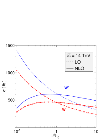
Figure 3: Scale dependence of the LO and NLO cross sections at the LHC. The curves with and without stars are for $W^{-}\gamma jj$ and $W^{+}\gamma jj$ productions, respectively. The reference scale $\mu_{0}$ is defined in Eq. (5) and the text.

At $\mu_{o}$ with this set up we obtain $\sigma_{LO}=622.7\,\pm\,0.1\,\mathrm{fb}$ $(457.6\,\pm\,0.1\,\mathrm{fb})$ and $\sigma_{NLO}=605.0\,\pm\,0.3\,\mathrm{fb}\,(459.6\,\pm\,1.2\,\mathrm{fb})$ for $W^{+}\gamma jj$ $(W^{-}\gamma jj)$ production, with the $W$ decaying into the first generation of leptons. Here the errors are the Monte Carlo errors of the calculation. The $K$-factor defined as $K\equiv\sigma_{NLO}/\sigma_{LO}$, is $0.97\,(1.00)$.

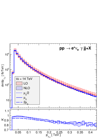
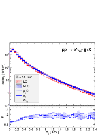
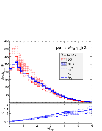
Figure 4: Differential cross sections, for QCD-induced $W\gamma jj$ production at LO and NLO, with inclusive cuts are shown for the transverse momenta of the hardest jet (top left) and the photon (top right), the invariant mass (bottom left) of the two tagging jets ordered by $p_{T}$. The distributions of the rapidity separation between the two jets are in the bottom right panel. The bands describe $\mu_{0}/2\leq\mu_{F}=\mu_{R}\leq 2\mu_{0}$ variations. The $K$-factor bands are due to the scale variations of the NLO results, with respect to $\sigma_{\text{LO}}(\mu_{0})$. The dots in the small panels are for the central scale, while the two solid lines correspond to $\mu_{F}=\mu_{R}=2\mu_{0}$ and $\mu_{0}/2$.

The result depends on the factorization and renormalization scales since we only calculate at fixed order in perturbative QCD. Fig. 3 shows, both for $W^{+}\gamma jj$ and $W^{-}\gamma jj$ production, that the dependence of the cross section on the factorization and renormalization scale, which are set equal for simplicity, is significantly reduced when calculating the NLO QCD corrections. If we vary the two scales separately, a small dependence on $\mu_{F}$ is observed, while the $\mu_{R}$ dependence is similar to the behavior shown in Fig. 3.

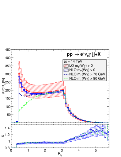
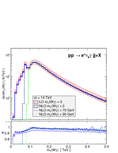
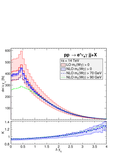
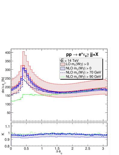
Figure 5: Differential cross sections, for the QCD-induced channels at LO and NLO, with inclusive cuts and for different values of the $m_{T,(W\gamma)}$ cut. In the upper row the distributions $R_{l\gamma}$ (left) and the transeverse cluster energy of the $W\gamma$ system $m_{T,(W\gamma)}$ (right) are shown. The lower row shows the rapidity (left) and azimuthal angle (right) separation of the photon and lepton. The bands on the distributions describe $\mu_{0}/2\leq\mu_{F}=\mu_{R}\leq 2\mu_{0}$ variations for $m_{T,(W\gamma)}>0$. The corresponding $K$-factor bands are due to the scale variations of the NLO results, with respect to $\sigma_{\text{LO}}(\mu_{0})$. The curves with stars in the narrow panels below the distributions are for the central scale for $m_{T,(W\gamma)}>0$. The $K$-factors at $\mu_{0}$ for the other cuts are also shown.

In the following, distributions for the $W^{+}\gamma jj$ production channel will be presented. The results for $W^{-}\gamma jj$ production are similar. Fig. 4 shows in the top row the differential LO and NLO cross sections of the transverse momentum of the hardest jet (left) and the photon (right), and in the lower row, the invariant mass (left) and rapidity separation (right) of the two tagging jets ordered by $p_{T}$. To give a measure of scale uncertainty, we also include with bands the results for $\mu_{F}=\mu_{R}=\mu=2^{\pm 1}\mu_{0}$. The small panels show the differential $K$-factors, defined as the ratio of the NLO to the LO results.

The differential distributions are less sensitive at NLO to the scale variation than at LO and the relative scale uncertainty is equally distributed in the entire $p_{T,j_{1}}$ and $p_{T,\gamma}$ spectrum. The phase space shows a non-trivial dependence with $K$-factors varying, for $\mu=\mu_{0}$, from $1.2$ to $0.8$ for the $p_{T}$ distribution of the hardest jet and from $0.95$ to $0.8$ for the transverse momenta of the photon in the ranges shown.

In the bottom panels, we observe a similar significant reduction of the scale uncertainties for the $m_{jj}$ (left) and the $\Delta y_{\text{tags}}$ (right) differential distributions, with the $K$-factor of the invariant mass distributions varying from about 0.9 to 1.2 at 2.4 TeV and with a fairly constant slope and the $K$-factor for the rapidity difference of the two leading tagging jets varying from 0.85 to 1.4 in the range showed.

Finally in Fig. 5, we plot in the left the differential distribution of the separation in the rapidity azimuthal-angle plane of the lepton and photon, $R_{l\gamma}$, and on the the right the transverse cluster mass of the $W\gamma$ system defined as (see e.g. Ref. Baur:1993ir )

$$m_{T,W\gamma}=\left(\left[(m_{l\gamma}^{2}+p_{T_{l\gamma}}^{2})^{\frac{1}{2}}+\displaystyle{\not}p_{T}\right]^{2}-({\boldsymbol{p}_{\boldsymbol{T}}}_{l\gamma}+{\displaystyle{\not}\boldsymbol{p}_{\boldsymbol{T}}})^{2}\right)^{\frac{1}{2}}.$$

In those plots, one can observe how the photon radiated off the lepton can be effectively removed by imposing a cut on the transverse cluster mass. This radiative W decay represents a simple QED process (bottom left diagram of Fig. 1), which diminishes the sensitivity to anomalous couplings, which might enter in e.g. the top left diagram of Fig. 1. For $m_{T,W\gamma}>90\,\mathrm{GeV}$, the radiative decay peak at $m_{T,W\gamma}=m_{W}$ is eliminated, affecting mainly the region of small $R_{l\gamma}$ (left). Furthermore, the NLO cross section is reduced by approximately 15% showing the efficiency of the cut.

The $R_{l\gamma}$ distribution in Fig. 5 shows a sudden increase of the $K$-factor starting at $\pi$, which correlates to the sudden fall of the differential cross section. This discontinuity in the slope can be explained as follows. The $R$ separation is defined as $R_{l\gamma}=[(\Delta y_{l\gamma})^{2}+(\Delta\phi_{l\gamma})^{2}]^{1/2}$ where $\Delta\phi_{l\gamma}\in[0,\pi]$. For $0<R_{l\gamma}<\pi$, the dominant contribution comes from the $\Delta y_{l\gamma}\approx 0$ region (see the $\Delta y_{l\gamma}$ distribution in Fig. 5), and the behavior of the $K$-factor is given by the one of the $\Delta\phi_{l\gamma}$ distribution also displayed in Fig. 5, which is rather flat. For $R_{l\gamma}>\pi$, the rapidity separation must increase and the $K$-factor is similar to the one of the $\Delta y_{l\gamma}$ distribution.

The above results for various differential distributions show that our default scale choice defined in Eq. (5) and the text can make the LO results quite similar to the NLO ones, with the difference being smaller than $20\%$ in most cases. The exceptional cases are the distributions of $\Delta y_{\text{tags}}$ (see Fig. 4) and $\Delta y_{l\gamma}$ (see Fig. 5). Here we observe that the $K$-factor increases with large rapidity separations. This indicates that the default scale choice is too large at large rapidity separations, making the LO results too small. We have tried a different scale choice, using Eq. (5) with $a=1/2$ and $b=0$, and found that the NLO results, for the distributions shown, agree with the ones obtained with the default scale within $10\%$, while the two scale choices at LO produce differences as large as a factor of 2 for the $m_{jj}$ and $\Delta y_{\text{tags}}$ distributions. We also found that the new scale choice makes the $K$-factors decrease well below one with increasing invariant mass or rapidity separation of the two hardest jets.

4 Conclusions

In this paper, we have reported first results for $W^{\pm}\gamma jj+X$ production at order $\mathcal{O}\!\left(\alpha_{s}^{3}\alpha^{3}\right)$, including the leptonic decays, full off-shell and finite width effects as well as all spin correlations. The NLO QCD corrections to the total cross section are small but they exhibit non-trivial phase space dependencies, reaching up to $40\%$, and lead to shape changes of the distributions. Hence, they should be taken into account for precise measurements at the LHC.

Our code will be publicly available as part of the VBFNLO program Arnold:2008rz ; Arnold:2012xn , thereby further studies of the QCD corrections with different kinematic cuts can be easily done.

Appendix A Results at one phase-space point

In this appendix, we provide results at a random phase-space point to facilitate comparisons with our results. We focus on the virtual amplitudes of the five benchmark subprocesses Eq. (2). The amplitudes of all other subprocesses can be obtained via crossing. The phase-space point for the process $j_{1}j_{2}\to j_{3}j_{4}e^{+}\nu_{e}\gamma$ is given in Table 1.

Table 1: Momenta (in GeV) at a random phase-space point for $j_{1}j_{2}\to j_{3}j_{4}e^{+}\nu_{e}\gamma$ subprocesses.

	$E$		$p_{x}$		$p_{y}$		$p_{z}$
$j_{1}$	32.	0772251055223	0.	0	0.	0	32.	0772251055223
$j_{2}$	2801.	69305619768	0.	0	0.	0	-2801.	69305619768
$j_{3}$	226.	525314156010	-10.	2177083492279	-1.	251308382450315$\times 10^{-15}$	-226.	294755550298
$j_{4}$	327.	281588297290	-6.	48554750244653	-10.	1061447270513	-327.	061219882068
$e^{+}$	646.	824307052136	36.	0746355875450	-26.	0379256562231	-645.	292438579767
$\nu_{e}$	1598.	85193997112	-2.	88431497177613	24.	4490976584709	-1598.	66239347157
$\gamma$	34.	2871318266438	-16.	4870647640944	11.	6949727248035	27.	6949763915464

Table 2: QCD interference amplitudes $2\text{Re}(\mathcal{A}_{\text{NLO}}\mathcal{A}^{*}_{\text{LO}})$ for $u\bar{d}\to\bar{u}ue^{+}\nu_{e}\gamma$ subprocess.

	$1/\epsilon^{2}$		$1/\epsilon$		finite
I operator	208.	754750693775	346.	823893959906	214.	565536875302
loop	-208.	754750694041	-346.	823893964206	1309.	48703231438
I+loop	-2.	661124653968727$\times 10^{-10}$	-4.	300034106563544$\times 10^{-9}$	1524.	05256918968

Table 3: QCD interference amplitudes $2\text{Re}(\mathcal{A}_{\text{NLO}}\mathcal{A}^{*}_{\text{LO}})$ for $u\bar{d}\to\bar{c}ce^{+}\nu_{e}\gamma$ subprocess.

	$1/\epsilon^{2}$		$1/\epsilon$		finite
I operator	204.	162116147897	338.	462143954872	193.	947096152034
loop	-204.	162116148143	-338.	462143959044	1250.	53101019255
I+loop	-2.	459898951201467$\times 10^{-10}$	-4.	172022727289004$\times 10^{-9}$	1444.	47810634458

Table 4: QCD interference amplitudes $2\text{Re}(\mathcal{A}_{\text{NLO}}\mathcal{A}^{*}_{\text{LO}})$ for $u\bar{d}\to\bar{d}de^{+}\nu_{e}\gamma$ subprocess.

	$1/\epsilon^{2}$		$1/\epsilon$		finite
I operator	211.	035586302262	351.	015498463760	217.	505955345503
loop	-211.	035586301469	-351.	015498460714	1288.	70122715328
I+loop	7.	927951628516894$\times 10^{-10}$	3.	046068286494119$\times 10^{-9}$	1506.	20718249878

Table 5: QCD interference amplitudes $2\text{Re}(\mathcal{A}_{\text{NLO}}\mathcal{A}^{*}_{\text{LO}})$ for $u\bar{d}\to\bar{s}se^{+}\nu_{e}\gamma$ subprocess.

	$1/\epsilon^{2}$		$1/\epsilon$		finite
I operator	204.	420606439876	338.	890671930900	194.	192653175338
loop	-204.	420606439076	-338.	890671927825	1255.	72258287559
I+loop	8.	000995421753032$\times 10^{-10}$	3.	075001586694270$\times 10^{-9}$	1449.	91523605093

Table 6: QCD interference amplitudes $2\text{Re}(\mathcal{A}_{\text{NLO}}\mathcal{A}^{*}_{\text{LO}})$ for $gg\to\bar{u}de^{+}\nu_{e}\gamma$ subprocess.

	$1/\epsilon^{2}$		$1/\epsilon$		finite
I operator	0.	134340391976220	1.	216201313632209$\times 10^{-2}$	0.	200038523086631
loop	-0.	134340391970929	-1.	216201313220419$\times 10^{-2}$	0.	164526176760187
I+loop	5.	291489468817190$\times 10^{-12}$	4.	117898730338077$\times 10^{-12}$	0.	364564699846818

In the following we provide the squared amplitude averaged over the initial-state helicities and colors. We also set $\alpha=\alpha_{s}=1$ for simplicity. The top quark is decoupled from the running of $\alpha_{s}$. However, its contribution is explicitly included in the one-loop amplitudes. At tree level, we have

$$\overline{|\mathcal{A}_{\text{LO}}^{u\bar{d}\rightarrow\bar{u}u}|}^{2} =245.933396692488,$$

$$\overline{|\mathcal{A}_{\text{LO}}^{u\bar{d}\rightarrow\bar{c}c}|}^{2} =240.522826586251,$$

$$\overline{|\mathcal{A}_{\text{LO}}^{u\bar{d}\rightarrow\bar{d}d}|}^{2} =248.620442839372,$$

$$\overline{|\mathcal{A}_{\text{LO}}^{u\bar{d}\rightarrow\bar{s}s}|}^{2} =240.827353287120,$$

$$\overline{|\mathcal{A}_{\text{LO}}^{gg\rightarrow\bar{u}d}|}^{2} =9.739448965670859\times 10^{-2}.$$ (7)

The interference amplitudes $2\text{Re}(\mathcal{A}_{\text{NLO}}\mathcal{A}^{*}_{\text{LO}})$, for the one-loop corrections (including counterterms) and the I-operator contribution as defined in Ref. Catani:1996vz , are given in Table 2, Table 3, Table 4, Table 5 and Table 6. Here we use the following convention for the one-loop integrals, with $D=4-2\epsilon$,

$$T_{0}=\frac{\mu_{R}^{2\epsilon}\Gamma(1-\epsilon)}{i\pi^{2-\epsilon}}\int d^{D}q\frac{1}{(q^{2}-m_{1}^{2}+i0)\cdots}.$$ (8)

This amounts to dropping a factor ${(4\pi)^{\epsilon}}/{\Gamma(1-\epsilon)}$ both in the virtual corrections and the I-operator. Moreover, the conventional dimensional-regularization method 'tHooft:1972fi with $\mu_{R}=M_{Z}$ is used. Changing from the conventional dimensional-regularization method to the dimensional reduction scheme induces a finite shift. This shift can be easily found by observing that the sum $|\mathcal{A}_{\text{LO}}|^{2}+2\text{Re}(\mathcal{A}_{\text{NLO}}\mathcal{A}^{*}_{\text{LO}})$ must be unchanged as explained in Ref. Catani:1996pk . Thus, the shift on
$2\text{Re}(\mathcal{A}_{\text{NLO}}\mathcal{A}^{*}_{\text{LO}})$ is opposite to the shift on the Born amplitude squared, which in turn is given by the following change in the strong coupling constant, see e.g. Ref. Kunszt:1993sd ,

$$\alpha_{s}^{\overline{DR}}=\alpha_{s}^{\overline{MS}}\left(1+\frac{\alpha_{s}}{4\pi}\right).$$ (9)

The shift on the I-operator contribution can easily be calculated using the rule given in Ref. Catani:1996vz .

References

- (1) B. Jager, C. Oleari, D. Zeppenfeld, JHEP 0607, 015 (2006). DOI 10.1088/1126-6708/2006/07/015
- (2) B. Jager, C. Oleari, D. Zeppenfeld, Phys.Rev. D73, 113006 (2006). DOI 10.1103/PhysRevD.73.113006
- (3) G. Bozzi, B. Jager, C. Oleari, D. Zeppenfeld, Phys.Rev. D75, 073004 (2007). DOI 10.1103/PhysRevD.75.073004
- (4) B. Jager, C. Oleari, D. Zeppenfeld, Phys.Rev. D80, 034022 (2009). DOI 10.1103/PhysRevD.80.034022
- (5) A. Denner, L. Hosekova, S. Kallweit, Phys.Rev. D86, 114014 (2012). DOI 10.1103/PhysRevD.86.114014
- (6) F. Campanario, N. Kaiser, D. Zeppenfeld, Phys.Rev. D89, 014009 (2014). DOI 10.1103/PhysRevD.89.014009
- (7) V. Hankele, D. Zeppenfeld, Phys.Lett. B661, 103 (2008). DOI 10.1016/j.physletb.2008.02.014
- (8) F. Campanario, V. Hankele, C. Oleari, S. Prestel, D. Zeppenfeld, Phys.Rev. D78, 094012 (2008). DOI 10.1103/PhysRevD.78.094012
- (9) G. Bozzi, F. Campanario, V. Hankele, D. Zeppenfeld, Phys.Rev. D81, 094030 (2010). DOI 10.1103/PhysRevD.81.094030
- (10) G. Bozzi, F. Campanario, M. Rauch, H. Rzehak, D. Zeppenfeld, Phys.Lett. B696, 380 (2011). DOI 10.1016/j.physletb.2010.12.051
- (11) G. Bozzi, F. Campanario, M. Rauch, D. Zeppenfeld, Phys.Rev. D84, 074028 (2011). DOI 10.1103/PhysRevD.84.074028
- (12) G. Bozzi, F. Campanario, M. Rauch, D. Zeppenfeld, Phys.Rev. D83, 114035 (2011). DOI 10.1103/PhysRevD.83.114035
- (13) K. Arnold, M. Bahr, G. Bozzi, F. Campanario, C. Englert, et al., Comput.Phys.Commun. 180, 1661 (2009). DOI 10.1016/j.cpc.2009.03.006
- (14) K. Arnold, J. Bellm, G. Bozzi, F. Campanario, C. Englert, et al., arXiv:1207.4975
- (15) A. Lazopoulos, K. Melnikov, F. Petriello, Phys.Rev. D76, 014001 (2007). DOI 10.1103/PhysRevD.76.014001
- (16) T. Binoth, G. Ossola, C. Papadopoulos, R. Pittau, JHEP 0806, 082 (2008). DOI 10.1088/1126-6708/2008/06/082
- (17) U. Baur, D. Wackeroth, M.M. Weber, PoS RADCOR2009, 067 (2010)
- (18) D.T. Nhung, L.D. Ninh, M.M. Weber, JHEP 1312, 096 (2013). DOI 10.1007/JHEP12(2013)096
- (19) T. Melia, K. Melnikov, R. Rontsch, G. Zanderighi, JHEP 1012, 053 (2010). DOI 10.1007/JHEP12(2010)053
- (20) T. Melia, P. Nason, R. Rontsch, G. Zanderighi, Eur.Phys.J. C71, 1670 (2011). DOI 10.1140/epjc/s10052-011-1670-x
- (21) B. Jager, G. Zanderighi, JHEP 1111, 055 (2011). DOI 10.1007/JHEP11(2011)055
- (22) F. Campanario, M. Kerner, L.D. Ninh, D. Zeppenfeld, arXiv:1311.6738
- (23) T. Melia, K. Melnikov, R. Rontsch, G. Zanderighi, Phys.Rev. D83, 114043 (2011). DOI 10.1103/PhysRevD.83.114043
- (24) N. Greiner, G. Heinrich, P. Mastrolia, G. Ossola, T. Reiter, et al., Phys.Lett. B713, 277 (2012). DOI 10.1016/j.physletb.2012.06.027
- (25) F. Campanario, M. Kerner, L.D. Ninh, D. Zeppenfeld, Phys. Rev. Lett. 111, 052003 (2013). DOI 10.1103/PhysRevLett.111.052003
- (26) T. Gehrmann, N. Greiner, G. Heinrich, arXiv:1308.3660
- (27) S. Badger, A. Guffanti, V. Yundin, arXiv:1312.5927
- (28) U. Baur, T. Han, J. Ohnemus, Phys.Rev. D48, 5140 (1993). DOI 10.1103/PhysRevD.48.5140
- (29) S. Frixione, Phys.Lett. B429, 369 (1998). DOI 10.1016/S0370-2693(98)00454-7
- (30) G. ’t Hooft, M. Veltman, Nucl.Phys. B44, 189 (1972). DOI 10.1016/0550-3213(72)90279-9
- (31) M.S. Chanowitz, M. Furman, I. Hinchliffe, Nucl.Phys. B159, 225 (1979). DOI 10.1016/0550-3213(79)90333-X
- (32) S. Catani, M. Seymour, Nucl.Phys. B485, 291 (1997). DOI 10.1016/S0550-3213(96)00589-5
- (33) G. ’t Hooft, M. Veltman, Nucl.Phys. B153, 365 (1979). DOI 10.1016/0550-3213(79)90605-9
- (34) Z. Bern, L.J. Dixon, D.A. Kosower, Nucl.Phys. B412, 751 (1994). DOI 10.1016/0550-3213(94)90398-0
- (35) S. Dittmaier, Nucl.Phys. B675, 447 (2003). DOI 10.1016/j.nuclphysb.2003.10.003
- (36) D.T. Nhung, L.D. Ninh, Comput. Phys. Commun. 180, 2258 (2009). DOI 10.1016/j.cpc.2009.07.012
- (37) A. Denner, S. Dittmaier, Nucl.Phys. B844, 199 (2011). DOI 10.1016/j.nuclphysb.2010.11.002
- (38) G. Passarino, M. Veltman, Nucl.Phys. B160, 151 (1979). DOI 10.1016/0550-3213(79)90234-7
- (39) A. Denner, S. Dittmaier, Nucl.Phys. B734, 62 (2006). DOI 10.1016/j.nuclphysb.2005.11.007
- (40) F. Campanario, JHEP 1110, 070 (2011). DOI 10.1007/JHEP10(2011)070
- (41) T. Binoth, J.P. Guillet, G. Heinrich, E. Pilon, C. Schubert, JHEP 0510, 015 (2005). DOI 10.1088/1126-6708/2005/10/015
- (42) T. Gleisberg, S. Hoeche, F. Krauss, M. Schonherr, S. Schumann, et al., JHEP 0902, 007 (2009). DOI 10.1088/1126-6708/2009/02/007
- (43) T. Gleisberg, S. Hoeche, JHEP 0812, 039 (2008). DOI 10.1088/1126-6708/2008/12/039
- (44) T. Hahn, Comput.Phys.Commun. 140, 418 (2001). DOI 10.1016/S0010-4655(01)00290-9
- (45) T. Hahn, M. Perez-Victoria, Comput. Phys. Commun. 118, 153 (1999). DOI 10.1016/S0010-4655(98)00173-8
- (46) K. Hagiwara, D. Zeppenfeld, Nucl.Phys. B313, 560 (1989). DOI 10.1016/0550-3213(89)90397-0
- (47) F. Campanario, C. Englert, M. Rauch, D. Zeppenfeld, Phys.Lett. B704, 515 (2011). DOI 10.1016/j.physletb.2011.09.072
- (48) F. Campanario, Q. Li, M. Rauch, M. Spira, JHEP 1306, 069 (2013). DOI 10.1007/JHEP06(2013)069
- (49) F. Campanario, M. Kubocz, Phys.Rev. D88, 054021 (2013). DOI 10.1103/PhysRevD.88.054021
- (50) A. Martin, W. Stirling, R. Thorne, G. Watt, Eur.Phys.J. C63, 189 (2009). DOI 10.1140/epjc/s10052-009-1072-5
- (51) M. Cacciari, G.P. Salam, G. Soyez, JHEP 0804, 063 (2008). DOI 10.1088/1126-6708/2008/04/063
- (52) S.D. Ellis, Z. Kunszt, D.E. Soper, Phys.Rev.Lett. 69, 1496 (1992). DOI 10.1103/PhysRevLett.69.1496
- (53) S. Catani, M. Seymour, Z. Trocsanyi, Phys.Rev. D55, 6819 (1997). DOI 10.1103/PhysRevD.55.6819
- (54) Z. Kunszt, A. Signer, Z. Trocsanyi, Nucl.Phys. B411, 397 (1994). DOI 10.1016/0550-3213(94)90456-1