Scale-dependent bias in the BAO-scale intergalactic neutral hydrogen

Abstract

I discuss fluctuations in the neutral hydrogen density of the $z\approx 2.3$ intergalactic medium and show that their relation to cosmic overdensity is strongly scale-dependent. This behaviour arises from a linearized version of the well-known “proximity effect”, in which bright sources suppress atomic hydrogen density. Using a novel, systematic and detailed linear-theory radiative transfer calculation, I demonstrate how Hi density consequently anti-correlates with total matter density when averaged on scales exceeding the Lyman-limit mean-free-path.

The radiative transfer thumbprint is highly distinctive and should be measurable in the Lyman-$\alpha$ forest. Effects extend to sufficiently small scales to generate significant distortion of the correlation function shape around the baryon acoustic oscillation peak, although the peak location shifts only by $1.2$ percent for a mean source bias of $b_{j}=3$. The distortion changes significantly with $b_{j}$ and other astrophysical parameters; measuring it should provide a helpful observational constraint on the nature of ionizing photon sources in the near future.

I Introduction

The Lyman-$\alpha$ forest Rauch98ARAA is the imprint of the intergalactic medium (IGM) – specifically, neutral hydrogen – on the spectra of distant quasars. At high redshift the rapidly-changing forest probes hydrogen reionization Becker01Reionization ; Fan02Reionization ; 2006ARA&A..44..415F ; at lower redshift, the forest has a steadier ionization state and is used to trace overall matter density fluctuations Croft02 ; McDonald03 ; BOSS_Slosar11 . Correlating Lyman-$\alpha$ fluctuations over small scales therefore places a strong constraint on modifications to the standard cold dark matter picture of structure formation Viel_WDM_Lya_2005 ; Viel_WDM_Lya_2008 ; Boyarsky_WDM_Lya_2009 . More recently attention has turned to the large-scale forest’s ability to constrain the baryon acoustic oscillation peak, providing an independent distance measurement for constraining dark energy Slosar09BAO ; BOSS_Slosar13 ; FontRibera_BOSS_QSO_Lya_X_BAO_2013 . In addition to probing the power spectrum in these ways, the observed $z<5$ forest constrains the thermal state of the intergalactic medium Becker07 ; Bolton08 , allowing various interesting processes to be studied (such as helium reionization Becker11HeIIreionization ).

When considering the forest after reionization, it is standard practice Croft98 ; McDonald00 ; McDonald03 to model the IGM ionization state in the presence of a uniform background of ultraviolet (UV) photons. Direct constraints on the Lyman-$\alpha$ cloud temperatures Bolton13IGMtemp dictate that collisional ionization is unimportant except in systems that are dense enough to be substantially self-shielded from the radiation.

However the assumption that the UV background is uniform is known to be incorrect, since the constituent photons are actually generated by galaxies and quasars. One can distinguish two limits in which the approximation fails. First, on small scales, quasars are rare; depending on the fraction of photons they contribute (likely around $50\%$ for $2<z<3$ Faucher-Giguere09_UVB ; HM12 ) they can add significant shot noise on small scales. Further fluctuations are imprinted by intrinsic variability in the IGM opacity Maselli05_LyA_transmissivity . This and related astrophysical effects have been widely investigated elsewhere Zuo92 ; Kollmeier03_LyA_LBG_connection ; Meiskin04_LyA_radiation ; Kollmeier06_LyA_galwinds ; Viel_WDM_Lya_2008 ; Slosar09BAO ; Mesinger09_LyA_fluctuating_reionisation ; White10_LyA_sims ; FontRibera_BOSS_QSO_Lya_X_2013 with the conclusion that, if properly accounted for, the added noise is not problematic for observational cosmology at $z<5$. Measurements at higher redshift, during the epoch of reionization, will be affected more strongly Meiskin04_LyA_radiation ; Mesinger09_LyA_fluctuating_reionisation as the UV undulation amplitude increases.

In this paper I will consider the post-reionization IGM and place more emphasis on a second failure of the uniform-radiation assumption. This appears only when source clustering is taken into account on scales around the mean-free-path of an ionizing photon. By definition, regions separated by greater distances cannot efficiently exchange UV radiation. Ionization equilibrium will therefore depend on the density of sources in the local region; the bias of the forest on the largest scales will depend on the clustering of UV sources Croft04_LyA_large_radiation ; McDonald05 ; McQuinn11_LyA_fluctuations ; White10_LyA_sims .

This effect has received less attention to date, probably because the relevant scale is seemingly extremely large (the mean-free-path is of order $500\,\mathrm{Mpc}$ in comoving units Rudie13MFP at $z=2.4$). In fact, once redshifting and volume dilution are accounted for, the transition scale is somewhat smaller (more like $350\,\mathrm{Mpc}$ comoving; see Section II.1). To fully model such scales would require exceptionally large radiative-transfer simulations, with box sizes exceeding a gigaparsec to properly probe long-wavelength fluctuations.

To achieve this, previous work has employed a combination of large dark-matter-only boxes and smaller hydrodynamic simulations Croft04_LyA_large_radiation or semi-analytic prescriptions McDonald05 . In the former case the author reported a significant drop in large-scale flux power out to scales of $k^{-1}\sim 70\,h^{-1}\,\mathrm{Mpc}$ relative to the homogeneous-radiation control case. Even so, the result has not received widespread attention. This is likely because extending such state-of-the-art work consumes a great deal of computer time and, furthermore, appropriate empirical constraints for such large separations have seemed out of reach.

The observational situation has now been changed radically by the BOSS (Baryonic Oscillation Spectroscopic Survey) project 2013Dawson_BOSS_overview . The team have released results demonstrating the viability of measuring the correlation function of Lyman alpha clouds on large scales BOSS_Slosar11 ; 2013_Busca_BOSS_Lya_BAO ; BOSS_Slosar13 . The major goal of BOSS is to measure the baryonic acoustic oscillation (BAO) feature in the correlation function at $100\,h^{-1}\,\mathrm{Mpc}$ comoving. This is not so far off the reduced mean-free-path scale discussed above and derived in Section II.1. It is timely, therefore, to reconsider the impact of large-scale fluctuations in the UV source density on the Lyman-$\alpha$ forest.

The remainder of this paper proceeds systematically from first principles to a detailed linear-theory calculation of these effects. This should be highly complementary to numerical studies, and motivate further work in the area. I will ignore observational questions such as the transformation from Hi to flux power spectrum, redshift-space distortions, redshift evolution and flux calibration biases – since these require major computational machinery in themselves 2013_Busca_BOSS_Lya_BAO ; BOSS_Slosar13 – and focus on the bias of the physical intergalactic Hi density at a single, fixed redshift. The quantitative results will be presented for $z=2.3$, around the mean redshift of observed Lyman-$\alpha$ clouds 2013_Busca_BOSS_Lya_BAO .

The approximations that allow this calculation to be completed are (i) that the spatial variations in the UV spectrum are less important for Hi than the changes in intensity (a ‘monochromatic approximation’); (ii) that the hydrogen can be split into a diffuse intergalactic component in photoionization equilibrium and a small population of self-shielded, collisionally-ionized clumps (i.e. the highest-column-density Lyman limit systems McQuinn_11_LyLimit ); (iii) that non-linear corrections (including quasar duty cycles) can be ignored on sufficiently large scales Slosar09BAO ; Mesinger09_LyA_fluctuating_reionisation ; White10_LyA_sims , although I will include shot noise from the rarity of sources; (iv) that sources averaged on large scales radiate isotropically. These seem reasonable to obtain a good estimate of the effects but in future they should be checked against numerical simulations and more complicated analytic treatments that allow for departure from equilibrium Zhang07_reion . After circulating a draft of this work, I was made aware of an independent study by Gontcho A Gontcho, Miralda-Escudè and Busca (in prep); at present it seems these authors reach many similar conclusions using a different calculation framework. This is encouraging, and it will be helpful to compare our approaches in due course.

Section II develops the inhomogeneous, monochromatic radiative transfer equations; Section III discusses the application of these equations to the large-scale, linear behaviour of intergalactic Hi. Section IV presents the main results, showing how various parameters change the distinctive imprint of radiative transfer on the intergalactic neutral hydrogen. Further discussion is given in Section V, especially in relation to observations of the Lyman-$\alpha$ forest. Two subsidiary issues are considered in appendices. In Appendix A, I re-derive all equations using general relativity, so including peculiar velocities and inhomogeneous gravitational redshifting and elucidating the gauge-dependence of the results (all of which considerations turn out to impact only on scales larger than those of interest here). Appendix B discusses the calibration of a particular parameter (the intergalactic Hi bias in the absence of radiation transfer) from analytic arguments and numerical simulations.

There are a few notational matters worth settling before starting the calculation. It is helpful to be able to decompose any quantity $X$ into its spatial mean value $X_{0}$ and fractional perturbations $\delta_{X}$ defined by

$$\delta_{X}=\frac{X-X_{0}}{X_{0}}\textrm{.}$$ (1)

Later I will mainly deal with the Fourier transform $\hskip 1.42262pt\tilde{\delta}_{X}$ of these fractional variations; any quantity can be re-written

$$\delta_{X}(\mathbf{x})=\frac{1}{(2\pi)^{3/2}}\int\mathrm{d}^{3}k\,e^{i\mathbf{k}\cdot\mathbf{x}}\hskip 1.42262pt\tilde{\delta}_{X}(\mathbf{k})\textrm{,}$$ (2)

where $\mathbf{k}$ is the comoving wavevector. Finally, the power spectrum $P_{X}(k)$ is defined by

$$\langle\hskip 1.42262pt\tilde{\delta}_{X}(\mathbf{k}^{\prime})^{*}\hskip 1.42262pt\tilde{\delta}_{X}(\mathbf{k})\rangle=P_{X}(k)\delta(\mathbf{k}-\mathbf{k}^{\prime})$$ (3)

where angle brackets denote an ensemble average and, by an unfortunate quirk of conventional notation, the $\delta$ on the right hand side represents the Dirac delta function. It follows from these definitions that the power spectrum for any quantity has units of a comoving volume. The expression above assumes statistical isotropy so that $P_{X}$ is a function of $k=|\mathbf{k}|$ alone.

Numerical results will be derived assuming a fiducial Planck temperature-only Planck13_CosmoPar cosmology $(h,\Omega_{M0},\Omega_{\Lambda 0})=(0.6711,0.3175,0.6825)$, where $\Omega_{M0}$ and $\Omega_{\Lambda 0}$ are the present day matter and cosmological constant densities relative to critical and $h=H_{0}/(100\,\mathrm{km}\,\mathrm{s}^{-1}\,\mathrm{Mpc}^{-1})$ is the dimensionless Hubble parameter today. The main role of these quantities will be to fix the Hubble expansion rate at $z=2.3$; any uncertainties are easily small enough to be ignored for the present study.

II Radiative Transfer

In this Section, I will derive a monochromatic approximation to the radiative transfer equation; this involves systematically integrating over frequency dependence. Because the scales of interest remain strongly sub-horizon, relativistic corrections will be sub-dominant and are excluded. For the interested reader, they are reintroduced in Appendix A which shows explicitly that they constitute a small correction.

To start, let $f(\mathbf{x},\mathbf{n},\nu)$ denote the physical number density of photons at comoving position $\mathbf{x}$ traveling in direction $\mathbf{n}$ with frequency $\nu$. In the absence of collisional effects, the total number of photons is conserved. However the Lagrangian phase volume that those photons occupy changes over time: the spatial volume increases as $a^{3}$ while the frequency interval decreases as $a$, giving an overall expansion rate of $a^{2}$. Overall, this implies the following Boltzmann equation:

$$\frac{\partial f}{\partial t}+\frac{c}{a}(\mathbf{n}\cdot\nabla)f+\frac{\partial f}{\partial\nu}\frac{\mathrm{d}\nu}{\mathrm{d}t}+2Hf=C[f]\textrm{,}$$ (4)

where $c$ is the speed of light, $a$ is the universe scalefactor and $H=\dot{a}/a$ is the usual Hubble expansion rate. $C[f]$ contains the collisional terms (i.e. those that alter the photon number) and will be expanded in a moment. In order, the terms on the left-hand-side denote the Eulerian rate of change of photon density; the free-streaming of photons; the redshifting of the photons; and the volume dilution discussed above. The gradient operator $\nabla$ is taken with respect to the comoving position $\mathbf{x}$ throughout this work. The term $\partial f/\partial t$ will now be set to zero, meaning I am approximating the radiation and ionization to be in equilibrium as noted in the Introduction. At the background level, this is a good approximation at $z=2.3$ – the evolution of the photoionization rate $\Gamma_{0}$ is slow, $\mathrm{d}\ln\Gamma_{0}/\mathrm{d}\ln a\approx-0.04$ from the tabulations of Ref. HM12 – but the implications of time-dependence for perturbations should certainly be explored further in future work.

To formulate the collisional term, consider first the emission of radiation. There are two distinct relevant aspects: first, galaxies and quasars generate energy from stars and black holes; second, the intergalactic Hi regenerates a fraction of photons it previously absorbed when the electron and proton recombine. I will treat these two terms separately in what follows.

Now consider absorption processes. A large effect will come from the IGM, corresponding to the low-column-density Lyman-$\alpha$ forest. The density of the neutral hydrogen $n_{\mathrm{HI}}(\mathbf{x})$ in this phase will be a key quantity. However, some portion (to be quantified later) of absorption comes from small, dense clumps which are strongly self-shielded against the UV radiation that is being modeled. At least three characteristics distinguish the clumped phase: first, the density of Hi is determined by collisional ionization and hence essentially unaffected by variations in the radiation. Second, the majority of recombination radiation produced is re-absorbed internally within a clump. Third, the amount of radiation absorbed by such a population does not scale with the mass of Hi in the population, but rather with the geometrical size and number density of the objects. For all three reasons, this population requires separate treatment.

Following the above discussion, the emission and absorption of photons can be expressed by

$$C_{\nu}\left[f\right]=j_{\nu}(\mathbf{x}) +n_{\mathrm{HI}}(\mathbf{x})\left(\frac{\Gamma(\mathbf{x})}{4\pi}f_{\mathrm{rec}}(\nu,T)-c\sigma_{\mathrm{HI}}\left(\nu\right)\,f\right)$$

$$-c\kappa_{\mathrm{clump}}(\mathbf{x},\nu)f\textrm{,}$$ (5)

where:

• $j_{\nu}(\mathbf{x},\mathbf{n})$ is the emissivity per unit physical volume per frequency interval from sources other than the IGM itself;

• $n_{\mathrm{HI}}(\mathbf{x})$ is the number of ground-state hydrogen atoms per unit physical volume in the IGM (excluding the shielded clumps);

• $\kappa_{\mathrm{clump}}(\mathbf{x},\nu)$ is the opacity from collisionally-ionized clumps;

• $f_{\mathrm{rec}}(\nu,T)$ is the IGM recombination spectrum, which depends on the temperature $T$ of the free electrons;

• $\Gamma(\mathbf{x})$ is the rate of ionization per Hi atom (and therefore also the recombination rate, assuming photoionization equilibrium); and

• $\sigma_{\mathrm{HI}}(\nu)$ is the cross-section of a Hi atom to ionization by a frequency $\nu$ photon.

In principle $j_{\nu}$ is a function of angle $\mathbf{n}$ as well as of position $\mathbf{x}$ but, in accordance with approximation (iv) above, the $\mathbf{n}$ dependence is now to be dropped (meaning that sources averaged over large scales radiate isotropically). I will also assume throughout that only Hi can absorb photons in the frequency range of interest.

The cross-section $\sigma_{\mathrm{HI}}$ is sharply peaked at the Lyman limit ($\nu_{\mathrm{LL}}\approx 3\times 10^{15}\,\mathrm{Hz}$), which allows for a monochromatic approach. The key quantity will be an effective number density of Lyman limit photons, $f_{\mathrm{LL}}$, defined by

$$f_{\mathrm{LL}}(\mathbf{x},\mathbf{n})=\int f(\mathbf{x},\mathbf{n},\nu)\sigma_{\mathrm{HI}}(\nu)\,\mathrm{d}\nu\textrm{.}$$ (6)

If desired, one can divide through by a fixed cross-section (e.g. $\sigma_{\mathrm{HI}}(\nu_{\mathrm{LL}})$) to “correct” the units of $f_{\mathrm{LL}}$, leading to cosmetic differences. Either way, $\sigma_{\mathrm{HI}}$ defines a single particular broad-band filter that we choose to focus on; the whole framework could be formulated in terms of another band if desired. This particular choice of filter is uniquely motivated because the ionization rate per Hi atom – a critical quantity of interest – is given exactly by integrating $f_{\mathrm{LL}}$ over all angles:

$$\Gamma(\mathbf{x})=c\iint f_{\mathrm{LL}}(\mathbf{x},\mathbf{n})\,\mathrm{d}^{2}n\textrm{.}$$ (7)

To obtain the Boltzmann equation for $f_{\mathrm{LL}}$, multiply equation (4) by $\sigma_{\mathrm{HI}}$ and integrate with respect to $\nu$, giving

$$a^{-1}(\mathbf{n}\cdot\nabla)f_{\mathrm{LL}}+\kappa_{\mathrm{tot}}f_{\mathrm{LL}}=c^{-1}\left(j+\bar{\sigma}_{\mathrm{HI}}n_{\mathrm{HI}}\frac{\Gamma}{4\pi}\beta_{\mathrm{r}}(T)\right)\textrm{,}$$ (8)

where $\kappa_{\mathrm{tot}}$ is an effective opacity, $j$ is an effective source emissivity and $\beta_{\mathrm{r}}(T)$ is a dimensionless, temperature-dependent fraction of recombination radiation which lies in our Lyman limit waveband. The formal definitions of these terms arise directly from the frequency integration, and will be given and discussed below in turn.

II.1 Absorption

First consider the effective opacity $\kappa_{\mathrm{tot}}$ which has been composed from separate diffuse IGM opacity, clump opacity, redshifting and volume dilution contributions:

$$\kappa_{\mathrm{tot}}=\bar{\sigma}_{\mathrm{HI}}n_{\mathrm{HI}}+\bar{\kappa}_{\mathrm{clump}}+\alpha_{z}\frac{H}{c}+3\frac{H}{c}\textrm{.}$$ (9)

I have written the volume term as $3H/c$ to directly associate it with comoving volume dilution; $\alpha_{z}$, a dimensionless number to be defined below, will contain a compensating term to return the $2H/c$ of the original formulation (4). The quantities $\bar{\sigma}_{\mathrm{HI}}$ and $\alpha_{z}$ are dependent on the spectrum, but not on the normalization of the spectrum; the monochromatic approach therefore assumes them independent of position. Their values can be estimated by using tabulated mean UV background estimates HM12 at $z=2.3$:

$$\bar{\sigma}_{\mathrm{HI}} =\frac{1}{f_{\mathrm{LL}}}\int\sigma_{\mathrm{HI}}^{2}f\,\mathrm{d}\nu\approx 3.87\times 10^{-18}\,\mathrm{cm}^{-2}\textrm{;}$$ (10)

$$\alpha_{z} =-\frac{1}{f_{\mathrm{LL}}}\int\sigma_{\mathrm{HI}}\frac{\partial f}{\partial\ln\nu}\,\mathrm{d}\nu-1\approx 1.57\textrm{.}$$ (11)

Meanwhile I have defined the monochromatic clump opacity

$$\bar{\kappa}_{\mathrm{clump}}(\mathbf{x})=\int\kappa_{\mathrm{clump}}(\mathbf{x},\nu)\,\sigma_{\mathrm{HI}}(\nu)\,\mathrm{d}\nu\textrm{.}$$ (12)

It will be convenient later to write the fraction of effective opacity from the respective terms as

$$\beta_{\mathrm{HI}}=\frac{\bar{\sigma}_{\mathrm{HI}}n_{\mathrm{HI}}}{\kappa_{\mathrm{tot}}}\textrm{; }\beta_{\mathrm{clump}}=\frac{\bar{\kappa}_{\mathrm{clump}}}{\kappa_{\mathrm{tot}}}\textrm{; }\beta_{z}=\frac{\alpha_{z}H}{c\kappa_{\mathrm{tot}}}\textrm{; }\beta_{V}=\frac{3H}{c\kappa_{\mathrm{tot}}}\textrm{.}$$ (13)

By definition these obey $\beta_{\mathrm{HI}}+\beta_{\mathrm{clump}}+\beta_{z}+\beta_{V}=1$. We can estimate their values by referring to the observational constraints on Lyman limit opacity; for instance Ref. Rudie13MFP quote a mean-free-path of $\kappa_{\mathrm{HI}}^{-1}\equiv(\bar{\sigma}_{\mathrm{HI}}n_{\mathrm{HI}}+\bar{\kappa}_{\mathrm{clump}})^{-1}\approx 150\,\mathrm{Mpc}$ in physical units at $z\approx 2.4$. Their value takes into account the intergalactic medium absorption alone (it excludes volume and redshifting effects, as well as circumgalactic absorption immediately around the emitting object). Correcting to $z=2.3$ using Rudie13MFP $\lambda_{\mathrm{MFP}}\propto(1+z)^{-4.5}$ and converting to comoving units gives a helpful reference value:

$$a^{-1}\kappa_{\mathrm{HI}}^{-1}\approx 570\,\mathrm{Mpc}\textrm{ comoving at }z=2.3\textrm{.}$$ (14)

There are uncertainties in the analysis of the observational data Prochaska13_MFP which could imply that the correct mean-free-path is somewhat longer than this value; results for different $\kappa_{\mathrm{HI}}$ will be investigated at the end of the work.

With the Planck cosmology defined in the introduction one has $H(z=2.3)/c\approx(1280\,\mathrm{Mpc})^{-1}$ and therefore, taking the reference value of $\kappa_{\mathrm{HI}}$ above,

$$\beta_{\mathrm{HI}}+\beta_{\mathrm{clump}}=0.62\textrm{; }\beta_{z}=0.13\textrm{; }\beta_{V}=0.25\textrm{.}$$ (15)

One immediate implication of these calculations is that, compared against physical opacity, redshifting and volume dilution are sub-dominant but important factors in lowering the cosmological density of Lyman-limit photons. This implies that the relevant scale at which scale-dependent effects are centered is smaller than the quoted Hi-only mean-free-path; we now have

$$a^{-1}\kappa_{\mathrm{tot}}^{-1}\approx 350\,\mathrm{Mpc}\textrm{ comoving at }z=2.3\textrm{.}$$ (16)

This is closer to the range measurable by BOSS. In fact when solving the equations in detail below, this characteristic path-length will turn out to be sufficiently short that radiation transfer can have a significant impact on the forest at the BAO scale.

Finally, one needs to decide how to assign opacity between the intergalactic Hi and clumps. Sadly there is no way to do this unambiguously so I will further parameterize:

$$p_{\mathrm{clump}}=\frac{\beta_{\mathrm{clump}}}{\beta_{\mathrm{clump}}+\beta_{\mathrm{HI}}}\textrm{.}$$ (17)

Ref. Rudie13MFP details the fraction of opacity from systems of differing column density, allowing an estimate of $p_{\mathrm{clump}}$. For a parcel of gas to count as clumped, the definition made above equation (5) requires it to be in collisional ionization equilibrium. The boundary will therefore be somewhat higher than the traditional Lyman limit system threshold because reaching the collisionally-ionized state requires a reduction in photoionization rate by a substantial fraction throughout the cloud.

The details depend strongly on the temperature, density and geometry of the system itself; here I will make a very rough order-of-magnitude estimate for a cut-off point. From the radiative-transfer simulations in Ref. PontzenDLA , I determined that a typical Lyman-limit system has an electron density around $10^{-2}\,\mathrm{cm}^{-3}$ and a temperature $T\approx 2.4\times 10^{4}\mathrm{K}$. This gives a collisional ionization rate of approximately Black81clouds $1.2\times 10^{-13}\mathrm{s}^{-1}$, compared to the photoionization rate HM12 of around $1.0\times 10^{-12}\mathrm{s}^{-1}$. One therefore needs to suppress the intergalactic flux by a factor of around ten to reach collisional ionization.

Then, making a simple uniform-density 1D model of a clump irradiated by the intergalactic flux, the mean flux inside as a function of total column density $N$ is given by $\Gamma_{0}(1-e^{-\bar{\sigma}_{\mathrm{HI}}N})/(\bar{\sigma}_{\mathrm{HI}}N)$. Note therefore that, although the central photoionization rate falls exponentially with $N$, the mean falls only approximately linearly with $N$. Accordingly for the mean rate to drop to $\Gamma_{0}/10$ requires $N\approx 10\bar{\sigma}_{\mathrm{HI}}^{-1}\approx(2.6\times 10^{18})\,\mathrm{cm}^{2}$. The cumulative effect of column densities greater than these limits constitute only around 10% of the IGM opacity (see Ref. Rudie13MFP , Figure 10). For that reason I will adopt $p_{\mathrm{clump}}=0.10$, showing the effect of varying the value at the end of the paper.

II.2 Recombination emission

Now let us turn attention to the recombination radiation term. This arises automatically from the integration discussed above equation (8), with the definition

$$\beta_{\mathrm{r}}(T)=\frac{1}{\bar{\sigma}_{\mathrm{HI}}}\int_{0}^{\infty}\sigma_{\mathrm{HI}}(\nu)f_{\mathrm{rec}}(\nu,T)\,\mathrm{d}\nu\textrm{,}$$ (18)

which provides a dimensionless measure of the amount of recombination radiation that ends up in the monochromatic waveband under consideration. Over the frequencies of interest, $f_{\mathrm{rec}}$ can be approximated as an offset Maxwell-Boltzmann distribution corresponding to the electron temperature $T$, scaled by the fraction of recombinations that occur directly to the ground state:

$$f_{\mathrm{rec}}(\nu,T)\approx 2hf_{\infty\to 1}\sqrt{\frac{h(\nu-\nu_{\mathrm{LL}})}{\pi(kT)^{3}}}e^{-h(\nu-\nu_{\mathrm{LL}})/kT}\textrm{,}$$ (19)

where $f_{\infty\to 1}\approx 0.40$ is the fraction of recombinations direct to the ground state loeb2013firstgals , $h$ is Planck’s constant and $k$ is Boltzmann’s constant. At $z\approx 2.4$ (close enough to our fiducial redshift), a typical forest temperature is Becker11HeIIreionization ; Bolton13IGMtemp $T=2.5\times 10^{4}\,\mathrm{K}$; evaluating equation (18) then gives $\beta_{\mathrm{r}}=0.39$. In principle, we could keep track of how variations in the mean temperature correlate with variations in the mean density; note, however, that when considering the averaged effects on linear scales this may not be the same as the equation of state measured for individual clouds Bolton13IGMtemp . Worse, large scale spatial temperature correlations could well be generated by unmodeled, non-equilibrium phenomena such as helium reionization Lai05_LyA_temp_flucs ; Bolton06_UV_shape_fluctuations ; Furlanetto09_He_fluc ; Becker11HeIIreionization . Luckily, the final effect of these on the photoionization equilibrium will be sub-dominant because $\beta_{\mathrm{r}}$ changes quite slowly with temperature ($\mathrm{d}\beta_{\mathrm{r}}/\mathrm{d}\ln T=-0.15$). The impact of thermal fluctuations on the recombination spectral shape is thus small compared to their effect on the recombination rate (which scales approximately as $T^{-0.7}$ in the intergalactic regime). Even in the latter case, within our monochromatic approximation the temperature variations do not depend strongly on the local ionizing field strength HuiGnedin97_IGM_EoS . Incorporating multi-wavelength, time-dependent radiative transfer could introduce qualitatively important corrections to the temperature field and should be prioritized in future work (see Section V).

II.3 Other sources

There is one remaining term in equation (8) that as-yet has not been discussed: $j(\mathbf{x})$. Recall that (8) is obtained by integrating (4) over frequency; accordingly $j(\mathbf{x})$ is defined by

$$j(\mathbf{x})=\int j_{\nu}(\mathbf{x})\,\sigma_{\mathrm{HI}}(\nu)\,\mathrm{d}\nu\textrm{,}$$ (20)

and specifically excludes the recombination emission which was treated separately above. Looking ahead in the calculation, we will need to understand the statistical properties of the $j(\mathbf{x})$ field. It is widely believed that, at $z\approx 2.3$, quasars and galaxies both contribute significantly to the UV emission HM12 . For both populations, systematic fluctuations $\delta_{j}$ are thought to be proportional to a constant (the ‘bias’, $b_{j}$) times the matter density fluctuations $\delta_{\rho}$ 2011PhRvD..84f3505B when averaged over suitably large scales. However we will also need to consider the shot noise: because quasars are rare, even a uniform distribution would have a significant Poisson fluctuation in density from place to place. In the limit of large scales (and therefore large numbers), these Poisson fluctuations can be modeled as an additive Gaussian noise, giving the total large-scale emissivity variations:

$$\delta_{j}(\mathbf{x})=b_{j}\,\delta_{\rho}(\mathbf{x})+\delta_{\mathrm{SN}}(\mathbf{x})\textrm{,}$$ (21)

where, in accordance with definition (1), $\delta_{\rho}(\mathbf{x})$ is the fractional matter overdensity determined by the cosmology and $\delta_{\mathrm{SN}}(\mathbf{x})$ is the uncorrelated shot-noise Gaussian random field. If multiple source populations contribute to the emissivity, they add linearly from which it follows that

$$\delta_{j}(\mathbf{x})=\sum_{i}\frac{j_{0,i}}{j_{0}}\left(b_{j,i}\,\delta_{\rho}(\mathbf{x})+\delta_{\mathrm{SN,i}}(\mathbf{x})\right)\textrm{,}$$ (22)

where the sum extends over the different source categories $i$ and the total mean emissivity is $j_{0}=\sum_{i}j_{0,i}$. Comparing equations (21) and (22) shows that the net large-scale effect is the same as that of a single population with suitably averaged parameters as I will discuss below.

Consider first the bias $b_{j}$, which is established by estimating the correlation strength of the emitting objects. Quasars are found to be strongly biased ($b_{q}\approx 4$) with respect to the matter density field Croom2dF_QSObias05 ; White_QSO_clustering . Galaxies are substantially less strongly correlated, and therefore less biased; Ref. Adelberger05_galaxy_correlation quotes a correlation length of $r_{0}=4.3\,h^{-1}\,\mathrm{Mpc}$ for a sample of bright ($23.5<\mathcal{R}<25.5$) galaxies at $z\approx 2.2$. This translates into a bias of $b_{g}\approx 2.4$ with the Planck cosmology described above, assuming the underlying matter fluctuations to be normalized Planck13_CosmoPar to $\sigma_{8}=0.834$ at $z=0$.

To add complication, these biases are measured for bright objects; especially in the case of galaxies, a significant fraction of photons are emitted from a large population of individually under-luminous objects Reddy09_UV_LF . To understand how the bias scales with luminosity one can assume it arises from the underlying dark matter halo. In that case the bias implies a halo mass ColeKaiser_Bias_89 ; for instance, with $b_{g}=2.4$ we obtain a characteristic mass of $M=4\times 10^{11}\,\mathrm{M}_{\odot}$. Suppose we wish to consider galaxies a factor of $10$ fainter than the sample of Ref. Adelberger05_galaxy_correlation ; then a number of arguments point to the dark matter halos being approximately a factor of $\sqrt{10}$ less massive Moster13 ; PontzenDLA . This can be translated back into a bias of $1.9$. Similarly, dropping another factor of $10$ in luminosity yields halos with bias $1.5$.

So the appropriate ‘source bias’ is sensitive to details of the underlying population generating the UV photons. For a combination of different sources, equation (22) shows that the net bias is exactly the average of the two individual biases, weighted by the emissivity of the populations. As a default value in this work, I will assume an average source bias of $b_{j}=3$, representing the average between highly biased quasars and a range of galaxy luminosities. (Recall that the value does not need to be further reduced for recombination emission, since that is included elsewhere in the calculation.) Reflecting the uncertainty, I will also show results for a range of $b_{j}$ from $1.5$ to $4.0$. A great attraction of future measurements of the effects in this paper is that they should in principle constrain $b_{j}$ and so shed light on the origin of UV photons.

Now consider the shot-noise term $\delta_{\mathrm{SN}}$ for a single population. This represents random variations in the density of sources. For a mean density of $\bar{n}$, the number of sources in a volume $V$ is given by

$$N(V)=\bar{n}\left(V+\frac{1}{(2\pi)^{3/2}}\int_{V}\mathrm{d}^{3}x\int\mathrm{d}^{3}k\,e^{i\mathbf{k}\cdot\mathbf{x}}\hskip 1.42262pt\tilde{\delta}_{\mathrm{SN}}(\mathbf{k})\right)\textrm{.}$$ (23)

Using this expression to demand that $\langle N^{2}\rangle-\langle N\rangle^{2}=N$ for any volume $V$ (the Gaussian, large-$N$ limit of Poisson noise) dictates the power spectrum

$$P_{\mathrm{SN}}(k)=\bar{n}^{-1}\textrm{,}$$ (24)

independent of scale, where $P_{\mathrm{SN}}(k)$ is defined by equation (3) and correctly has units of comoving volume as explained earlier. The shot-noise is modeled as stationary; in fact quasars likely have a finite duty cycle, causing the realization of the shot-noise to change over time. The effect of this cannot be analyzed rigorously with the time-stationary approach I have adopted, but it could plausibly change the impact of noise on large scales. It should therefore be investigated in future work.

Just as for the bias $b_{j}$, choosing an appropriate value of $\bar{n}$ is tricky. One can start by parameterizing the quasar luminosity function $\Phi(L)$ using a double power-law fit (e.g 2007ApJ…654..731H, ; Ross13_SDSS9_QLF, ); following the consequences of equation (21) for a series of infinitesimal bins in luminosity, assuming an independent shot-noise realization for each bin, one is led to an $L^{2}$-weighted Mesinger09_LyA_fluctuating_reionisation ; McQuinn11_LyA_fluctuations effective quasar number density defined by

$$\bar{n}_{q}=\frac{\left(\int\Phi(L)\,L\,\mathrm{d}L\right)^{2}}{\int\Phi(L)\,L^{2}\,\mathrm{d}L}\textrm{.}$$ (25)

Since the intrinsic luminosity function in the ionizing radiation is unknown (being completely obscured by Lyman limit absorption) I assume that the ionizing radiation of a given quasar scales linearly with its bolometric luminosity. Evaluating equation (25) using estimates for the bolometric population parameters 2007ApJ…654..731H then gives $\bar{n}_{q}$ between $1.5\times 10^{-6}$ and $10^{-5}\,\mathrm{Mpc}^{-3}$ comoving over the parameter range quoted by Ref 2007ApJ…654..731H .

As with $b_{j}$, the $\delta_{\mathrm{SN}}$ appearing in equation (21) can be seen from equation (22) to be a photon-weighted average of the $\delta_{\mathrm{SN}}$ appropriate to the two populations. The density of galaxies is so much higher that one can essentially ignore their shot-noise contribution compared to that of the quasars. Tracing this through, assuming again a 50% contribution from both populations, one has to multiply $\bar{n}$ by 4 to account for the galaxy part of the emission (since $\delta_{\mathrm{SN}}$ scales with $\bar{n}^{-1/2}$). This yields the approximate upper limit $\bar{n}\approx 4\times 10^{-5}\,\mathrm{Mpc}^{-3}\approx 10^{-4}\,h^{3}\,\mathrm{Mpc}^{-3}$, with a lower limit of $2\times 10^{-5}\,h^{3}\,\mathrm{Mpc}^{-3}$. To be clear, the $\bar{n}$ derived in this way is not the density of any particular population – it is a weighted average which accounts for the very different densities of two populations.

These estimates neglect any effects of time-variability and anisotropy which will introduce qualitative corrections and possibly lead to an increase in the effective $\bar{n}$ by pushing observed variation to smaller scales. I will therefore adopt the upper end of the naive uncertainty for the present. Results will later be shown for a full range of possible $\bar{n}$. Many of the same physical considerations bear on the value of both $\bar{n}$ and $b_{j}$, but I will consider them to be separate parameters for the sake of clarity.

The total power spectrum for the sources $P_{j}(k)$ is just

$$P_{j}(k)=b_{j}^{2}P_{\rho}(k)+\bar{n}^{-1}\textrm{,}$$ (26)

which follows because, by assumption, $\langle\hskip 1.42262pt\tilde{\delta}_{\rho}(\mathbf{k})\hskip 1.42262pt\tilde{\delta}_{\mathrm{SN}}(\mathbf{k}^{\prime})\rangle=0$. A similar expression was given by Ref. McQuinn11_LyA_fluctuations . However, despite appearing on an equal footing in equation (26), the shot-noise and correlated components behave differently in terms of their effect on the Hi White10_LyA_sims , as we will see below.

III Linearization

The preceding section concluded by discussing the behaviour of sources averaged on large scales in terms of spatial perturbations $\delta$ defined by (1). The plan now is to rewrite the radiative transfer equations in terms of $\delta$’s. Ignoring all terms of order $\delta$ yields the homogeneous or “zero-order” approximation; the Boltzmann equation (8) becomes (integrating over all angles without loss of information)

$$\kappa_{\mathrm{tot},0}(1-\beta_{\mathrm{HI}}\beta_{\mathrm{r}})\Gamma_{0}=4\pi j_{0}\textrm{,}$$ (27)

which expresses the equilibrium condition that the overall rate of photon production is balanced by the effective absorption from redshifting, dilution and ionization.

Expanding equation (8) to linear order and simplifying using the background solution (27), one obtains an expression for $\hskip 1.42262pt\tilde{\delta}_{f_{\mathrm{LL}}}$:

$$\hskip 19.91684pt\hskip 1.42262pt\tilde{\delta}_{f_{\mathrm{LL}}}=\frac{(1-\beta_{\mathrm{HI}}\,\beta_{\mathrm{r}})\,\hskip 1.42262pt\tilde{\delta}_{j}+\beta_{\mathrm{HI}}\,\beta_{\mathrm{r}}\,\left[\hskip 1.42262pt\tilde{\delta}_{n_{\mathrm{HI}}}+\hskip 1.42262pt\tilde{\delta}_{\Gamma}\right]-\hskip 1.42262pt\tilde{\delta}_{\kappa_{\mathrm{tot}}}}{i(a\kappa_{\mathrm{tot},0})^{-1}\,(\mathbf{n}\cdot\mathbf{k})+1}\textrm{,}$$ (28)

where I have suppressed functional $\mathbf{k}$ and $\mathbf{n}$ dependencies for brevity. Excepting small gravitational effects (Appendix A), the effective opacity fluctuations $\delta_{\kappa_{\mathrm{tot}}}$ are linked solely to variations in the diffuse and clumped neutral hydrogen:

$$\delta_{\kappa_{\mathrm{tot}}}=\beta_{\mathrm{HI}}\delta_{n_{\mathrm{HI}}}+\beta_{\mathrm{clump}}\delta_{\bar{\kappa}_{\mathrm{clump}}}\textrm{.}$$ (29)

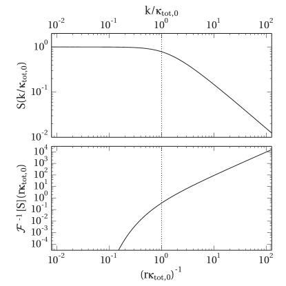
Figure 1: In the linear approximation, the radiative transfer consists of convolving an effective source function (including emission, absorption and re-radiation terms) with a kernel S, equation (30). The kernel is shown here in Fourier space (upper panel) as a function of wavenumber divided by $\kappa_{\mathrm{tot},0}$. On large scales (toward the left) $S(k)$ is $\approx 1$, meaning fluctuations in the effective source function are tracked by fluctuations in the number density of ionizing photons. On small scales (toward the right), $S(k)$ decays towards zero; fluctuations in the photon density are suppressed and the uniform UV approximation will apply. The lower panel shows the same kernel transformed into real space; the horizontal axis is an inverse distance, so the two panels read in the same direction.

Integrating out the remaining angular dependence in equation (28), noting that $\int\mathrm{d}^{2}n\,\hskip 1.42262pt\tilde{\delta}_{f_{\mathrm{LL}}}=4\pi\hskip 1.42262pt\tilde{\delta}_{\Gamma}$, one obtains an implicit equation for $\hskip 1.42262pt\tilde{\delta}_{\Gamma}$:

$$\hskip 1.42262pt\tilde{\delta}_{\Gamma}(\mathbf{k}) =\left[(1-\beta_{\mathrm{HI}}\,\beta_{\mathrm{r}})\,\hskip 1.42262pt\tilde{\delta}_{j}-\beta_{\mathrm{HI}}\,(1-\beta_{\mathrm{r}})\,\hskip 1.42262pt\tilde{\delta}_{n_{\mathrm{HI}}}\right.$$

$$\left.\hskip 56.9055pt-\beta_{\mathrm{clump}}\,\hskip 1.42262pt\tilde{\delta}_{\bar{\kappa}_{\mathrm{clump}}}+\beta_{\mathrm{HI}}\,\beta_{\mathrm{r}}\,\hskip 1.42262pt\tilde{\delta}_{\Gamma}\right]S(k)\textrm{,}$$

$$S(k) =\frac{a\kappa_{\mathrm{tot},0}}{k}\arctan\frac{k}{a\kappa_{\mathrm{tot},0}}\textrm{,}$$ (30)

showing the characteristic scale-dependence arising in the radiation field (Figure 1, upper panel). Performing an inverse Fourier transform on the kernel $S(k)$ returns the radial function $e^{-\kappa_{\mathrm{tot},0}r}/r^{2}$ (Figure 1, lower panel). The systematic approach has therefore recovered something like the heuristic equations of Refs Mesinger09_LyA_fluctuating_reionisation ; McQuinn11_LyA_fluctuations , where sources are convolved with a similar kernel. However, those works do not take into account the shortened effective mean-free-path from redshifting and volume-dilution contributions (they use $\kappa_{\mathrm{HI}}$ where $\kappa_{\mathrm{tot},0}$ is more appropriate). Moreover the appearance of $\hskip 1.42262pt\tilde{\delta}_{n_{\mathrm{HI}}}$ (from inhomogeneous absorption) and $\hskip 1.42262pt\tilde{\delta}_{\Gamma}$ (from recombination radiation) on the right-hand-side of equation (30) means that the convolution kernel is modified from this simple form once absorption fluctuations, as well as emission fluctuations, are included.

	Spectrum-dependent coefficients
$\alpha_{z}$	Coefficient for background redshifting (11)	$1.57$
$\beta_{\mathrm{r}}$	Fraction of Hi recombinations to LL photons (18)	$0.39$
	Estimated origin of effective opacity $\kappa_{\mathrm{tot},0}$, eq. (13)
$\beta_{\mathrm{HI}}$	Fraction from Hi in photoionization equilibrium	$0.56$
$\beta_{\mathrm{clump}}$	Fraction from collisional-equilibrium clumps	$0.06$
$\beta_{z}$	Fraction from redshifting	$0.13$
$\beta_{V}$	Fraction from dilution	$0.25$
	Input biases relative to the linear overdensity field
$b_{\mathrm{HI,u}}$	Bias of Hi in homogeneous radiation limit	$1.5$
$b_{j}$	Bias of photon source objects	$3$
$b_{j,\mathrm{eff}}$	Effective bias of sources including recombination (33)	$2.6$

Table 1: Dimensionless quantities used in this work, with a brief a explanation and the default value calculated or estimated at $z=2.3$.

On large scales $S(k\to 0)$ is $\approx 1$, meaning fluctuations in the effective source function are tracked by fluctuations in the number density of ionizing photons. This agrees with the intuitive picture outlined earlier, in which regions separated by more than the mean-free-path must arrive at independent ionization equilibria. On small scales $S(k\to\infty)$ decays towards zero; fluctuations in the photon density are suppressed and the uniform UV approximation is recovered. (On sufficiently small scales one will, however, have enhanced non-linear shot noise; as discussed in the introduction I will consider only the linear regime in the present work.)

We are now in a position to understand the mean ionization state. Recalling that the effects of shielded clumps have already been dealt with – the $n_{\mathrm{HI}}$ field refers specifically to the intergalactic Hi alone – we can write

$$\delta_{n_{\mathrm{HI}}}=\delta_{n_{\mathrm{HI}},\mathrm{u}}-\delta_{\Gamma}\textrm{,}$$ (31)

where $\delta_{n_{\mathrm{HI}},\mathrm{u}}$ describes the Hi field in the case of a completely uniform ionizing background; the given relationship is a consequence of linearizing the photo-ionization equilibrium equation $n_{\mathrm{HI}}\propto 1/\Gamma$. In the absence of any radiative fluctuations, by definition $\delta_{n_{\mathrm{HI}}}=\delta_{n_{\mathrm{HI}},\mathrm{u}}$. Combining equation (30) and (31) gives a solution for $\hskip 1.42262pt\tilde{\delta}_{n_{\mathrm{HI}}}$ in terms of $\hskip 1.42262pt\tilde{\delta}_{j}$, $\hskip 1.42262pt\tilde{\delta}_{n_{\mathrm{HI}},\mathrm{u}}$ and $\hskip 1.42262pt\tilde{\delta}_{\bar{\kappa}_{\mathrm{clump}}}$:

$$\hskip 1.42262pt\tilde{\delta}_{n_{\mathrm{HI}}}=\frac{\hskip 1.42262pt\tilde{\delta}_{n_{\mathrm{HI}},\mathrm{u}}-\left[(1-\beta_{\mathrm{HI}}\beta_{\mathrm{r}})\,\hskip 1.42262pt\tilde{\delta}_{j}-\beta_{\mathrm{clump}}\hskip 1.42262pt\tilde{\delta}_{\bar{\kappa}_{\mathrm{clump}}}+\beta_{\mathrm{HI}}\,\beta_{\mathrm{r}}\,\hskip 1.42262pt\tilde{\delta}_{n_{\mathrm{HI}},\mathrm{u}}\right]S(k)}{1-\beta_{\mathrm{HI}}\,S(k)}\textrm{.}$$ (32)

Now assume that $\hskip 1.42262pt\tilde{\delta}_{n_{\mathrm{HI}},\mathrm{u}}$ (the Hi density fluctuations in a completely uniform UV field), $\hskip 1.42262pt\tilde{\delta}_{j}$ (the source density fluctuations) and $\hskip 1.42262pt\tilde{\delta}_{\bar{\kappa}_{\mathrm{clump}}}$ (the self-shielded clump opacity fluctuations) can be written as a bias (respectively $b_{\mathrm{HI,u}}$, $b_{j}$ and $b_{\mathrm{clump}}$) times the fiducial cosmic density field, and further define an effective source bias

$$b_{j,\mathrm{eff}}=(1-\beta_{\mathrm{HI}}\,\beta_{\mathrm{r}})\,b_{j}-\beta_{\mathrm{clump}}\,b_{\mathrm{clump}}+\beta_{\mathrm{HI}}\,\beta_{\mathrm{r}}\,b_{\mathrm{HI,u}}\textrm{,}$$ (33)

which takes into account the recombination emission from the IGM and absorption from the clumps. The intergalactic Hi density then follows immediately,

$$\hskip 17.07182pt\hskip 1.42262pt\tilde{\delta}_{n_{\mathrm{HI}}}=\frac{\left[b_{\mathrm{HI,u}}-b_{j,\mathrm{eff}}\,S(k)\right]\hskip 1.42262pt\tilde{\delta}_{\rho}-\left[1-\beta_{\mathrm{HI}}\,\beta_{\mathrm{r}}\right]S(k)\,\hskip 1.42262pt\tilde{\delta}_{\mathrm{SN}}}{1-\beta_{\mathrm{HI}}\,S(k)}\textrm{,}$$ (34)

using equation (21). The Hi density perturbation $\hskip 1.42262pt\tilde{\delta}_{n_{\mathrm{HI}}}$ can be split into two terms, corresponding to the correlated and shot-noise components respectively. The correlated part obeys $\hskip 1.42262pt\tilde{\delta}_{n_{\mathrm{HI}}}=b_{\mathrm{HI}}\hskip 1.42262pt\tilde{\delta}_{\rho}$ where

$$b_{\mathrm{HI}}(k)=\frac{b_{\mathrm{HI,u}}-b_{j,\mathrm{eff}}\,S(k)}{1-\beta_{\mathrm{HI}}\,S(k)}\textrm{,}$$ (35)

showing that the Hi density traces the cosmological density in a scale-dependent way. This is the main result of the present work. Its implications will be discussed in the next section.

IV Results

IV.1 Bias and power spectrum

The preceding section used a systematic linearization of first-principles radiative transfer to derive equations governing the IGM Hi density on large scales. I will now explore what this implies for the bias $b_{\mathrm{HI}}$ (35) and total power spectrum. As previously discussed, a number of uncertain parameters enter the calculation, namely: the IGM bias in the uniform radiation limit, $b_{\mathrm{HI,u}}$; the effective source density $\bar{n}$; the effective source bias $b_{j}$; the fraction of opacity in collisionally-ionized clumps $p_{\mathrm{clump}}$; and the mean physical Lyman-limit opacity $\kappa_{\mathrm{HI}}=(\beta_{\mathrm{HI}}+\beta_{\mathrm{clump}})\kappa_{\mathrm{tot},0}$. This section will explore the consequences of varying all of these except for $b_{\mathrm{HI,u}}=1.5$ (see Appendix B for details). I will explore substantial variations around the default choices (justified earlier in the text) of $b_{j}=3$, $\bar{n}=10^{-4}h^{3}\,\mathrm{Mpc}^{-3}$, $p_{\mathrm{clump}}=0.10$ and $(a\kappa_{\mathrm{HI}})^{-1}=570\,\mathrm{Mpc}$ comoving.

The top panel of Figure 2 plots $b_{\mathrm{HI}}$ against comoving wavenumber $k$, equation (35). This represents the linear relationship between Hi density and total density as a function of scale. The dashed and solid lines show respectively the assumed relationship when there are no effects of inhomogeneous radiation and the calculated relationship for the default parameters.

The basic functional form and its $b_{j}$ dependence can be understood as follows. On small scales ($k\gg\kappa_{\mathrm{tot},0}$), $S(k)$ asymptotes to zero, so

$$b_{\mathrm{HI}}(k\gg\kappa_{\mathrm{tot},0})=b_{\mathrm{HI,u}}\textrm{,}$$ (36)

showing that the small modes are unaffected by radiative transfer phenomena at the linear level. Conversely on large scales, $S(k)$ asymptotes to one, giving

$$b_{\mathrm{HI}}(k\ll\kappa_{\mathrm{tot},0})=\frac{b_{\mathrm{HI,u}}-b_{j,\mathrm{eff}}}{1-\beta_{\mathrm{HI}}}$$ (37)

For $b_{j,\mathrm{eff}}>b_{\mathrm{HI,u}}$, this makes the Hi negatively biased on large scales, i.e. anti-correlated with the total density. The intensity of the radiation in dense regions over-compensates for the clustering of hydrogen, causing a net deficit in neutral hydrogen – a direct analogue of the proximity effect but averaged over many sources on large scales.

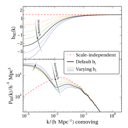
Figure 2: (Upper panel) the calculated bias of intergalactic Hi at $z=2.3$ as function of comoving wavenumber. The dashed line shows the bias in the uniform-radiation case; the solid line shows the bias calculated with radiative transfer. On small scales (towards the right), the calculated bias agrees with that of the uniform case. On large scales, the Hi is negatively biased because overdensities imply high emissivity, high radiation density and hence net Hi under-density. Dotted lines show the effect of changing the source bias $b_{j}$; from top to bottom, $b_{j}=1.5$, $2.0$, $\cdots$, $4.0$. (Lower panel) the corresponding power spectrum, $P_{\mathrm{HI}}(k)$, defined by equation (38), has a strong feature where $b_{\mathrm{HI}}$ passes through zero (near to $k=\kappa_{\mathrm{tot},0}^{-1}$).

This has profound consequences for the power spectrum of Hi fluctuations. Recall that $\hskip 1.42262pt\tilde{\delta}_{\mathrm{SN}}$ and $\hskip 1.42262pt\tilde{\delta}_{\rho}$ are uncorrelated, so we have

$$P_{\mathrm{HI}}(k)=b_{\mathrm{HI}}(k)^{2}P(k)+\left[\frac{(1-\beta_{\mathrm{HI}}\,\beta_{\mathrm{r}})\,S(k)}{1-\beta_{\mathrm{HI}}S(k)}\right]^{2}\frac{1}{\bar{n}}\textrm{.}$$ (38)

This power spectrum is plotted in the lower panel of Figure 2, with the default value $\bar{n}=5\times 10^{-4}h^{3}\,\mathrm{Mpc}^{-3}$ (Section II.3) and a fiducial $P(k)$ for the Planck cosmology calculated using CAMB Lewis:1999bs . The strong feature arises because $b_{\mathrm{HI}}^{2}$ touches zero at $k^{-1}\approx 125h^{-1}\,\mathrm{Mpc}$ comoving (for the default parameters). Accordingly there is a sharp dip in $P(k)$ around that wavenumber. On larger scales still, at the far left of Figure 2, the Hi fluctuations become stronger than predicted in the scale-independent model. This arises from a mixture of shot-noise (discussed in more detail below) and the large magnitude of the limiting bias (37).

Dotted lines in Figure 2 explore the impact of changing $b_{j}$ over a wide range; from top to bottom, $b_{j}=1.5$, $2.0$, $\cdots$, $4.0$. Recall that, as discussed in Section II.3, the source bias $b_{j}$ is composed of a photon-weighted average of different populations (excluding recombination emission, which is accounted for elsewhere within the calculation). As the source bias increases, the effects at a given wavenumber typically become stronger. Consequently the zero in $b_{\mathrm{HI}}$ moves to larger wavenumbers (shorter distances), making the radiation thumbprint more observationally accessible. Even for small biases, however ($b_{j}=1.5$) the effects are significant on scales of tens to hundreds of megaparsecs comoving.

On sufficiently small scales, the Hi power spectrum is unaffected by radiative transfer, regardless of the value of $b_{j}$. In particular, 1D measurements of the Lyman alpha forest are limited by the small path length that can be observed with an individual quasar. Only wavenumbers greater than $\sim 0.02s\,\mathrm{km}^{-1}$, corresponding to $2\,h\,\mathrm{Mpc}^{-1}$ comoving at $z=2.3$, are measured McDonald_SDSS_1DLyA_Pk_2006 ; from Figure 2 it is clear that the effects are minimal for such measurements. (The non-linear, non-Gaussian contribution to the shot noise on those scales will become significant, but plausibly average out over many sightlines Slosar09BAO ; White10_LyA_sims .)

IV.2 Auto- and cross-correlation function

To test the large-scale predictions against observations one must turn to more recent 3D analyses that take advantage of modern surveys with dense background sources 2013Dawson_BOSS_overview . In this context, it is more conventional to consider the correlation function $\xi(\mathbf{r})=\langle\delta(\mathbf{x}+\mathbf{r})\delta(\mathbf{x})\rangle$. It has been widely used to constrain the BAO feature in Lyman-$\alpha$ and other large scale structure tracers 2013_Busca_BOSS_Lya_BAO ; BOSS_Slosar13 ; BOSS_Anderson13_BAOGals . By isotropy $\xi$ is actually a function of $r=|\mathbf{r}|$ alone; one can show it is related to the power spectrum via a Legendre transformation,

$$\xi_{\mathrm{HI}}(r)=\frac{1}{2\pi^{2}}\int\mathrm{d}k\,\frac{\sin kr}{kr}k^{2}P_{\mathrm{HI}}(k)\textrm{.}$$ (39)

The correlation function for the Lyman-$\alpha$ flux $\xi_{F}$ is closely related to $\xi_{\mathrm{HI}}$ and can be measured from observations relatively directly. As explained in the introduction, this paper will not go as far as calculating $\xi_{F}$, but a brief discussion of the relationship to $\xi_{\mathrm{HI}}$ is given in Section V.

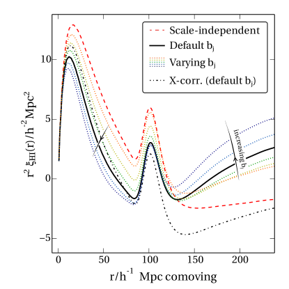
Figure 3: The correlation function of intergalactic Hi at $z=2.3$, as defined by the Legendre transform (39) of the power spectrum shown in Figure 2. As before, dashed lines show the constant bias case, whereas the solid line shows the calculated bias for inhomogeneous radiation (in the default case, $b_{j}=3.0$). The dotted lines show a series of different source biases ($b_{j}=1.5$, nearest the dashed line; then $2.0$, $2.5$, $3.5$ and $4.0$). The result of cross-correlating the Hi against a tracer population with fixed bias is shown by the dash-dotted line.

Figure 3 shows $\xi_{\mathrm{HI}}$ (renormalized by $r^{2}$ to highlight the BAO structure) for the scale-free (dashed line) and default radiation model (solid line). Once again the dotted lines show the calculated correlation function for a range of different source biases $b_{j}$ from $1.5$ to $4.0$. The mapping from power spectrum to correlation function causes a substantial mixing of information on different scales, so the new shape needs a little unpicking to understand. On scales smaller than $\sim 5\,h^{-1}\,\mathrm{Mpc}$, the scale-free predictions are barely altered; this corresponds to the small-scale limit $b_{\mathrm{HI}}\to b_{\mathrm{HI,u}}$ in the bias, Figure 2. Moving to larger separations, the radiation-corrected correlation function falls rapidly compared to the scale-free counterpart, because the Hi bias is declining and the power on these scales is suppressed. In fact, the new correlation function turns negative at around $55\,h^{-1}\,\mathrm{Mpc}$; this is an artifact of the constraint that $\int\xi(r)r^{2}\mathrm{d}r=0$ for a properly mean-calibrated sample, and the negativity in itself does not indicate anything physically special about these scales.

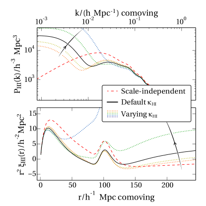
Figure 4: The effect of varying the mean Hi opacity on the power spectrum (upper panel) and correlation function (lower panel). Other parameters are held fixed. The dashed and solid lines show the uniform-radiation and reference case respectively, so agreeing with the same lines in Figures 2 and 3. Dotted lines show the results for an Hi opacity $0.25$, $0.5$, $2$ and $4$ times that of the default case. As the opacity increases, the mean-free-path decreases, meaning that the “dip” feature in the Hi power spectrum moves to shorter wavenumbers. Consequently small-scale power is increasingly suppressed, whereas large-scale power is enhanced.

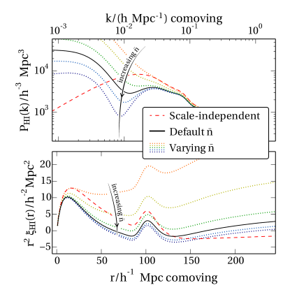
Figure 5: The effect of source shot-noise on the power spectrum (upper panel) and correlation function (lower panel). Other parameters are held fixed. The dashed and solid lines show the uniform-radiation and reference case respectively, so agreeing with the same lines in Figures 2 and 3. The dotted lines show the results for (top to bottom) $\bar{n}=10^{-5}$, $5\times 10^{-5}$, $10^{-4}$, $5\times 10^{-4}$ (solid line), $10^{-3}$ and $5\times 10^{-3}\,h^{3}\,\mathrm{Mpc}^{-3}$. As the effective source density $\bar{n}$ decreases, the amplitude of shot-noise increases, confusing the Hi signal. The changes are strongest on large scales for the reasons discussed in the text.

The BAO feature – a hump at around $r=100\,h^{-1}\,\mathrm{Mpc}$ – remains clearly visible in all cases, but the local maximum in $r^{2}\xi(r)$ shifts marginally. The local maximum can be found at $100.0\,h^{-1}\,\mathrm{Mpc}$ in the homogeneous case (dashed line) but at $101.2\,h^{-1}\,\mathrm{Mpc}$ in the fiducial $b_{j}=3.0$ case (solid line). At distances exceeding $130\,h^{-1}\,\mathrm{Mpc}$, the new correlation function begins to rise because of contributions from the increased power on very large scales (far left of Figure 2).

In cross-correlation, the signature looks slightly different. As an illustration, the dot-dashed line in Figure 3 shows a hypothetical cross-correlation against a fixed-bias population with $b=1.5$ (this value has no significance except to scale the overall function similarly to the auto-correlation). In other words, I am plotting $\xi_{\mathrm{HI}\times}\equiv 1.5\langle\delta_{\mathrm{HI}}(\mathbf{x}+\mathbf{r})\delta_{\rho}(\mathbf{x})\rangle$. In simple cases this would return the geometric mean of the dashed and solid lines. However, there are a couple of more subtle effects here. First, the negativity of the Hi bias on large scales reduces the large-distance cross-correlation ($\xi_{\mathrm{HI}\times}$ probes $b_{\mathrm{HI}}$ whereas $\xi_{\mathrm{HI}}$ is sensitive only to $b_{\mathrm{HI}}^{2}$). Second, the plot assumes cross-correlation against a population other than quasars so that the shot-noise term cancels. Overall this leads to a cross-correlation that is suppressed more strongly on large scales than would be expected from an averaging argument.

IV.3 Varying other parameters

So far I have only shown results for varying $b_{j}$. However there are other parametric dependencies which ought to be examined. The first is the physical Hi opacity, $\kappa_{\mathrm{HI}}$, which is the inverse of the mean-free-path of a photon in the absence of redshifting or volume-dilution. The default value has been discussed extensively above; in Figure 4 I have shown what happens when $\kappa_{\mathrm{HI}}$ is changed by a factor of $0.25$, $0.5$, $2$ and $4$. The actual uncertainty in the observationally-constrained value Rudie13MFP ; Prochaska13_MFP is more likely under a factor of 2. The upper and lower panels show the power spectrum and correlation function respectively. Solid and dashed lines therefore correspond exactly to those presented in Figures 2 and 3; the dotted lines show the impact of changing $\kappa_{\mathrm{HI}}$. As this opacity increases (i.e. the mean-free-path decreases), the effects becomes more prominent on smaller scales. A slightly more subtle change occurs at long wavelengths: as the mean-free-path decreases, the large-scale limiting bias increases, as does the noise contribution. Since $\beta_{\mathrm{HI}}$ increases when $H$ is fixed but $\kappa_{\mathrm{HI}}$ increases, this behaviour is in accordance with equation (37). Physically, photo-ionized Hi amplifies fluctuations in radiation on large scales: an overdensity of radiation implies a lower Hi fraction and therefore a deficit in opacity, in turn boosting the overdensity of radiation. This is why, as $\kappa_{\mathrm{HI}}$ increases, the fluctuations on large scales become more dramatic.

Next consider the effect of varying $\bar{n}$ from its fiducial value. Recall that this determines the large-scale shot-noise contribution and is related to the underlying source population densities (Section II.3). Fixing the other parameters, Figure 5 demonstrates the effect of $\bar{n}$ varying between $5\times 10^{-3}\,h^{3}\,\mathrm{Mpc}^{-3}$ and $10^{-5}\,h^{3}\,\mathrm{Mpc}^{-3}$ on the power spectrum (upper panel) and auto-correlation function (lower panel). Smaller source densities lead to a stronger effect, with significant power added in the case of $\bar{n}=10^{-5}\,h^{3}\,\mathrm{Mpc}^{-3}$. It may come as a surprise that, in all cases, the effects of low source density are most pronounced as $r$ becomes large (or $k$ small) rather than in the opposite limit. In the linear, averaged limit, however, this is correct. The shot-noise power spectrum is suppressed on small scales by $S(k)^{2}$ which declines steeply at increasing $k$ (Figure 1). The intuitive picture that shot-noise matters more on small scales depends on the transition to the non-linear, unaveraged regime which I have not attempted to model.

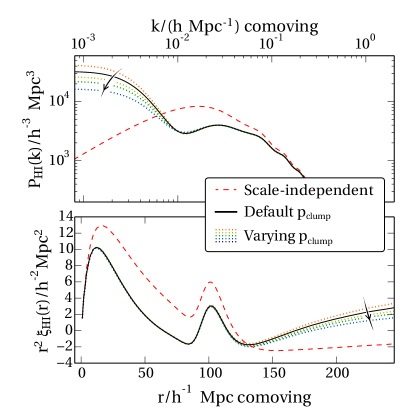
Figure 6: The effect of changing the fraction of opacity from collisionally-ionized clumps on the power spectrum (upper panel) and correlation function (lower panel). Other parameters are held fixed. The dashed and solid lines show the uniform-radiation and reference case respectively, so agreeing with the same lines in Figures 2 and 3. The dotted lines show the results for (top to bottom) $p_{\mathrm{clump}}=0.0$, $0.1$ (solid line), $0.2$, $\cdots$, $0.5$. When more opacity arises from clumps (higher $p_{\mathrm{clump}}$), the effect of radiation is slightly weaker because the clumps are able to partially counterbalance the enhanced radiation in overdense regions. However, the effect is minor.

Finally let us return to the parameter $p_{\mathrm{clump}}$, which controls the fraction of opacity arising from self-shielded, collisionally-ionized clumps as opposed to diffuse, photo-ionized Hi. As this parameter is increased, $\beta_{\mathrm{HI}}$ decreases and $\beta_{\mathrm{clump}}$ increases. The overall effects are shown in Figure 6 for $p_{\mathrm{clump}}=0.0$, $0.1$ (the default), $0.2$, $\cdots$, $0.5$. For scenarios with a greater fraction of opacity in clumps, the effect of radiation is slightly mitigated on very large scales. However the differences are minor.

For realistic observations, the effects of $p_{\mathrm{clump}}$ will be somewhat larger: here I am plotting the effect only on the photo-ionized intergalactic medium. Increasing the fraction of clumps contributing to the Lyman-limit opacity will also increase the balance of such systems in the Lyman-$\alpha$ forest flux spectrum. Since they are collisionally ionized, they are not much affected by the inhomogeneous radiation field and therefore they dilute the scale-dependent effects roughly by a fraction $1-p_{\mathrm{clump}}$. In other words, the leading-order effect of a large $p_{\mathrm{clump}}$ on observations will be different to, and more important than, the physical effect on the intergalactic Hi which I have discussed here.

Nonetheless, whatever the value of any of these parameters, there are substantial changes to the intergalactic Hi correlation function at all scales exceeding $5\,h^{-1}\,\mathrm{Mpc}$. It seems likely that these should be detectable with BOSS observations of the Lyman-$\alpha$ forest – even if observational complications lead to a substantial dilution. This prospect is considered further in the discussion below.

V Discussion

Radiative transfer imprints dramatic scale-dependent bias in the intergalactic Hi and therefore the Lyman-$\alpha$ forest, even after reionization is complete. This follows because regions separated by distances larger than the UV photon mean-free-path reach essentially independent photoionization equilibria. Source clustering is stronger than IGM clustering, leading to negative Hi bias on large scales (i.e. the Hi anti-correlates with large-scale overdensities).

This paper has presented a detailed calculation of these new effects by adopting a monochromatic, equilibrium, large-scale description, focusing on the large-scale, average correlations Croft04_LyA_large_radiation ; McDonald05 ; McQuinn11_LyA_fluctuations rather than small-scale non-linear fluctuations Viel_WDM_Lya_2008 ; Slosar09BAO . The systematic analytic treatment starts from first-principles radiative transfer and produces, with minimal computational effort, predictions for very large scales.

The calculation reveals, as expected from the argument above, a strong feature in the Hi power spectrum and a corresponding distortion of its correlation function. According to the estimates here, this distortion should have an effect at the BAO scale ($\approx 100\,h^{-1}\,\mathrm{Mpc}$). The BAO bump position is slightly shifted – in Figure 3, the local maximum is at 1.2% larger scales in the radiative-transfer case (solid line) compared to the constant-bias case (dashed line). That said, future cosmology constraints are unlikely to come from measuring the peak in such a simple way; so long as algorithms marginalize over possible broadband distortions to the correlation function, they will likely still recover an unbiased estimate of the BAO scale.

The most interesting conclusion is therefore that BAO-focused Lyman-$\alpha$ observational programmes will be able to recover helpful astrophysical constraints: the radiative transfer distortions are strongly dependent on the mean bias of sources (Figures 2 and 3), the Hi opacity (Figure 4) and the effective number density of sources $\bar{n}$ (Figure 5). As $b_{j}$ increases, the correlated component of the radiative fluctuations grows and the power on BAO scales decreases while the power on very large scales increases; as $\bar{n}$ decreases, the random component of the radiative fluctuations grows and the power on all scales increases. These trends seem to agree with numerical results where a comparison can be made Croft04_LyA_large_radiation ; McDonald05 ; McQuinn11_LyA_fluctuations .

The overall picture gives rise to a large number of questions. The most obvious is whether existing BOSS observations of the Lyman-$\alpha$ forest are compatible with the expected thumbprint. A variety of subtle observational issues must be taken into account before this can be answered. First, converting an Hi correlation function into a flux correlation function is a non-linear process that needs at a minimum to be calibrated by suitable numerical simulations McDonald03 . Redshift-space distortions will mix the dynamical growth of structure with the tracer statistics into a final observed correlation function 1987MNRAS.227….1K ; 1999coph.book…..P ; McDonald03 . Dependent on the exact survey design, angular binning and data cuts, these effects could easily dilute the scale-dependence, making the observed correlation function closer to the homogeneous-radiation result. However the changes in the underlying intergalactic Hi bias are sufficiently dramatic for it to seem implausible that the radiation-transfer signature would be obscured completely in forthcoming precision data. To be sure we will have to understand how the data processing and parameter degeneracies impact on our ability to measure the effects. Although the distortion is large, it is also a very smooth function of scale and therefore one needs to accurately calibrate the normalization of the correlation function over a wide range of scales to make a definitive detection; otherwise the effects are degenerate with a renormalization of the uniform-limit bias $b_{\mathrm{HI,u}}$.

The BOSS team have emphasized that their 3D Lyman-$\alpha$ forest pipeline is presently designed to pick out localized correlation-function features – i.e. the BAO bump – rather than reconstruct the entire function accurately 2013_Busca_BOSS_Lya_BAO ; BOSS_Slosar13 . Nonetheless an attempt to measure scale-dependence in cross-correlation against quasars has been made; none was found FontRibera_BOSS_QSO_Lya_X_2013 . Conversely some scale-dependence in the cross-correlation between damped Lyman alpha systems and the forest can be seen in the plots of Ref. 2012FontRibera_BOSS_DLA_Forest_X . It is unclear whether and how these results can be reconciled with the present work; observational difficulties such as continuum determination cause severely correlated errors in correlation functions and dealing with these leads to certain large-scale modes being projected out 2013_Busca_BOSS_Lya_BAO ; BOSS_Slosar13 . Overall, the task of determining whether the effects of radiative transfer are present in existing data is considerable. However, I hope that the present calculation has underlined the rewards of such an effort. The scale-dependent radiative transfer contains a rich, valuable source of information on the nature of UV sources.

21cm emission studies will not be affected by these considerations because the Hi they probe is largely in collisional- rather than photo-ionization equilibrium PontzenDLA . The 21cm absorption forest would be affected in just the same way as the Lyman-$\alpha$ forest; but this phenomena is of most promise at high redshift before or during reionization Pritchard21cm_review – so the present calculation does not apply. One way to tackle the larger fluctuations at high redshift is to use a halo-model-based calculation Furlanetto04_reion_model ; alternatively, a linear theory approach has been taken to the problem by Ref. Zhang07_reion ; Aloisio13_reion_fNL ; Mao13_reion_fNL . In these cases, an explicit time integration needs to be performed to follow the growth of ionized bubbles whereas in the present case the integration is absent because I have assumed equilibrium, making the present paper’s calculations considerably simpler but more restricted in scope.

Depending on one’s assumptions (for instance on the relative importance of quasars to the UV background, and on the quasar luminosity function), the rarity of sources also have a substantial impact on very large scales. Here I have modeled the resulting shot noise by a Gaussian approximation similar to that of Ref. McQuinn11_LyA_fluctuations ; in that work, noise was considered to be so large that the correlated component of the radiation fluctuations was thrown out of the calculation. In the present work the effects of shot-noise seem milder, which reflects that I work at lower redshift (where the comoving density of quasars has increased) and make greater allowance for a UV contribution from star-forming galaxies. Crucially, the correlated component has a qualitatively different signature to the noise component of the radiation field: the former reduces the power of Hi fluctuations on large scales, whereas the latter can only ever add power (at any scale). One effect that is absent from the present work concerns scales below $10\,\mathrm{Mpc}$ or so – here the noise would be significantly amplified Mesinger09_LyA_fluctuating_reionisation by 2-halo and other nonlinear effects. Another missing aspect from my analysis is that of time-dependence which could, for example, add further confusion from quasar duty cycles.

With all this in mind it would be of great interest to supplement the linear theory calculations of this work by revisiting the BAO-scale correlation function of the Lyman-$\alpha$ forest using non-linear numerical simulations of gigaparsec chunks of the IGM with correlated sources, incorporating radiative transfer – along the lines of work described by Refs Croft04_LyA_large_radiation ; McDonald05 ; McQuinn11_LyA_fluctuations . Hints of the anti-correlation discussed at length in the present paper have been seen before in such efforts Croft04_LyA_large_radiation ; White10_LyA_sims . It would be helpful to include large scale temperature fluctuations arising from helium reionization Furlanetto09_He_fluc . Or, one might be able to tackle temperature fluctuations analytically by relaxing the monochromatic assumption; it is worth re-emphasizing that the current work includes the zero-order effects of hard photons (the spectral shape enters through equation (11)), but not first-order changes from local fluctuations in spectral shape. At this level of approximation, the gas thermal equilibrium is nearly unaffected by radiation intensity fluctuations HuiGnedin97_IGM_EoS because the radiative heating rate can be approximately re-written as a function of density and temperature (via the ionization equilibrium condition). To answer the important question of how thermal fluctuations change the large-scale signal one therefore needs either to incorporate multi-wavelength radiative transfer or go beyond an equilibrium approximation – or, preferably, both HuiGnedin97_IGM_EoS .

Further work is required to reach a unified view of how radiation changes the observational prospects for cosmology and astrophysics with the Lyman-$\alpha$ forest. The present investigation forms a first guide to the effects that will dominate on the largest scales.

Appendix A Once more with gravity

The plan for this Appendix to regenerate equation (8) but now including peculiar velocity and gravitational inhomogeneities in accordance with general relativity. In fact, all the effects turn out to be minor on scales of interest: dimensionless perturbations to the metric $\phi$ are going to be small compared to the dimensionless perturbations $\hskip 1.42262pt\tilde{\delta}$ to the matter except on scales comparable to or larger than the horizon:

$$\phi(\mathbf{k})\sim\frac{3H_{0}^{2}\Omega_{m,0}(1+z)}{2c^{2}k^{2}}\hskip 1.42262pt\tilde{\delta}(\mathbf{k})\approx\frac{4.2\,\mathrm{Gpc}^{-2}}{k^{2}}\hskip 1.42262pt\tilde{\delta}(\mathbf{k})\textrm{,}$$ (40)

where, as in the main text, $k$ is the comoving wavenumber. If you are convinced by this argument, there is no need to read any further.

On the other hand, factors arising from spectral integrations could outweigh the scale contrast and make the effects relevant. To be sure either way one needs to press ahead with the calculation. I work in conformal Newtonian gauge to make the geodesic equations relatively simple, but will briefly discuss the effect of gauge changes at the end of this Appendix. The formal derivation starts with a suitably perturbed flat Friedmann-Robertson-Walker (FRW) universe described by the metric 1992PhR…215..203M ,

$$\mathrm{d}s^{2}=-(1+2\psi)c^{2}\mathrm{d}t^{2}+a(t)^{2}(1-2\phi)\mathrm{d}\mathbf{x}^{2}\textrm{,}$$ (41)

where $t$ is coordinate time, $\psi$ and $\phi$ are the scalar potentials, and $\mathbf{x}$ are the comoving position coordinates.

Consider a photon with wavevector $k_{\mu}$ traveling through this perturbed metric. The null condition $k_{\mu}k^{\mu}=0$ implies that (working throughout at first order in the potentials)

$$\frac{\mathrm{d}\mathbf{x}}{\mathrm{d}t}=\frac{c}{a}(1+\psi+\phi)\mathbf{n}\textrm{,}$$ (42)

where $\mathbf{n}$ is the unit vector in the spatial propagation direction. The observed frequency of the photon in the coordinate frame is $\nu=ck^{0}(1+\psi)$; combining this with the geodesic equation for $k^{\mu}$ one finds that

$$\frac{\mathrm{d}\nu}{\mathrm{d}t}=\nu\left(-H-\frac{c}{a}\mathbf{n}\cdot\nabla\psi+\dot{\phi}\right)\textrm{.}$$ (43)

I will assume that on large scales all absorber and emitter streaming velocities follow that of the pressureless dark matter. The tangent 4-vector $u^{\mu}$ with $u_{\mu}u^{\mu}=-1$ can be related to the peculiar velocity $\mathbf{v}$ as

$$u^{\mu}=c^{-1}\left(\begin{array}[]{c}1-\psi\\ \mathbf{v}/a\\ \end{array}\right)\textrm{,}$$ (44)

where I have used a new assumption that $|\mathbf{v}|/c$ is small (the same order as the potentials). The frequency of the photon as seen by an absorber is then

$$\nu^{\prime}\equiv-u^{\mu}k_{\mu}\approx\nu\left[1-\mathbf{n}\cdot\frac{\mathbf{v}}{c}\right]\textrm{,}$$ (45)

again at first order. Finally, the physical 3-volume of a fixed $\mathbf{x}$ coordinate patch is proportional to $a^{3}(1-3\phi)$.

To define what is meant by an equilibrium solution to the Boltzmann equation in the relativistic setting, consider the rate of change $\dot{f}$ of the distribution function along a dark matter worldline. We have:

$$\dot{f}=cu^{\mu}f_{,\mu}\approx(1-\psi)\frac{\partial{f}}{\partial{t}}+\frac{\mathbf{v}\cdot\nabla f}{a}\textrm{,}$$ (46)

and since the gradient term is overall second order, we can again adopt the simple assumption that $\partial f/\partial t=0$ to obtain a well-defined equilibrium at first order, independent of gauge.

Putting this together, the underlying number density $f$ of photons satisfies the collisional Boltzmann equation,

$$\frac{c}{a}(1+\phi+\psi)(\mathbf{n}\cdot\nabla)f+\frac{\partial f}{\partial\nu}\frac{\mathrm{d}\nu}{\mathrm{d}t}+\left(\frac{\mathrm{d}\ln\Delta V\Delta\nu}{\mathrm{d}t}\right)f=C_{\nu^{\prime}}[f]\textrm{,}$$ (47)

where $C_{\nu^{\prime}}[f]$ is calculated according to equation (5) as before, but evaluated at the Doppler-shifted frequency $\nu^{\prime}$ according to equation (45); $\nabla$ again means the ordinary derivative with respect to comoving spatial coordinates $\mathbf{x}$, and I have taken $\partial f/\partial t=0$ as explained above. The quantity $\Delta V\Delta\nu$ appears because $f$ is expressed in photons per unit physical volume per unit frequency. A bundle of photons which occupies a volume $\Delta V\Delta\nu$ in this space at one moment will occupy a different volume at the next. The evolution of $\Delta V$ can be calculated by setting up an initially cubic volume with edges $\mathbf{\Delta x}^{(\parallel)}$, $\mathbf{\Delta x}^{\perp 1}$ and $\mathbf{\Delta x}^{\perp 2}$ such that $\mathbf{\Delta x}^{\parallel}$ is parallel to $\nabla(\psi+\phi)$ and the others are perpendicular. Then

$$\Delta V =a^{3}(1-3\phi)\Delta\mathbf{x}^{\parallel}\cdot\left(\Delta\mathbf{x}^{\perp 1}\times\mathbf{\Delta x}^{\perp 2}\right)$$ (48)

$$\Rightarrow\frac{\mathrm{d}\Delta V}{\mathrm{d}t} =\frac{\mathrm{d}\Delta\mathbf{x}^{\parallel}}{\mathrm{d}t}\cdot\left(\Delta\mathbf{x}^{\perp 1}\times\mathbf{\Delta x}^{\perp 2}\right)a^{3}(1-3\phi)+3\Delta V(H-\dot{\phi})$$

$$=\Delta V\left(\frac{c}{a}\mathbf{n}\cdot\nabla(\psi+\phi)+3H-3\dot{\phi}\right)$$ (49)

at first order, with other terms canceling from the choice of $\mathbf{\Delta x}$ vectors. Along with the frequency factor, which follows immediately from equation (43), the overall volume term then reads

$$\frac{\mathrm{d}\ln\Delta V\Delta\nu}{\mathrm{d}t}=2(H-\dot{\phi})+\frac{c}{a}\mathbf{n}\cdot\nabla\phi\textrm{.}$$ (50)

To link the gravitational effects to the perturbed density field $\rho$, we require the Einstein equations. The energy-momentum tensor for the pressureless, matter-dominated universe is

$$T_{\mu\nu}=\rho_{0}(1+\delta_{\rho})u_{\mu}u_{\nu}$$ (51)

We will work at sufficiently high redshift that we can take $\Lambda=0$. The zero-order Einstein equations recover the Friedmann and acceleration equations for the pressureless fluid universe; the linear-order equations reduce to

$$\phi =\psi$$ (52)

$$c^{2}\nabla(\dot{\phi}+H\phi) =-4\pi G\rho_{0}av(\mathbf{x})$$ (53)

$$c^{2}\nabla^{2}\phi =4\pi G\rho_{0}a^{2}\delta_{\rho}+3a^{2}H\left(\dot{\phi}+H\phi\right)$$ (54)

$$0 =\ddot{\phi}+4H\dot{\phi}$$ (55)

Equation (55) is solved by $\dot{\phi}=0$ (the potential is frozen, which corresponds to putting the matter perturbation $\delta_{\rho}$ in the growing mode); substituting also the zero-order Friedmann equation $3H^{2}/c^{2}=8\pi G\rho$ we have

$$(-2c^{2}\nabla^{2}+6a^{2}H^{2})\phi =-3a^{2}H^{2}\delta_{\rho}$$ (56)

$$\textrm{and }3aH\mathbf{v} =-2c^{2}\nabla\phi\textrm{.}$$ (57)

Let us now follow exactly the same procedure as in Sections II and III to obtain our previous approximation but with the relativistic terms present. Multiply equation (47) by $\sigma_{\mathrm{HI}}$ and integrate over all frequencies; then, comparing against equation (8) at linear order, only two extra terms survive. In particular, the perturbation to $\mathrm{d}\mathbf{x}/\mathrm{d}t$ is irrelevant because there are no spatial gradients in the background. Of the two remaining terms, first consider how the peculiar velocities induce an extra term on the right hand side:

$$\int C_{\nu^{\prime}}[f]\sigma_{\mathrm{HI}}\mathrm{d}\nu \approx\int C_{\nu}[f]\sigma_{\mathrm{HI}}\mathrm{d}\nu-\frac{\mathbf{n}\cdot\mathbf{v}}{c}\alpha_{v}Hf_{\mathrm{LL}}\textrm{,}$$ (58)

$$\textrm{where }\alpha_{v} =\frac{1}{Hf_{\mathrm{LL}}}\int\frac{\partial C_{\nu}[f]}{\partial\ln\nu}\sigma_{\mathrm{HI}}\mathrm{d}\nu\textrm{;}$$ (59)

the first term is the same as in our original calculation. The integral in the second term need be evaluated only at zero-order, for which we can use the background (zero-order) Boltzmann equation (47) in the form

$$\frac{1}{H}\frac{\partial C_{\nu}[f_{0}]}{\partial\ln\nu}=2\frac{\partial f_{0}}{\partial\ln\nu}-\frac{\partial^{2}f_{0}}{\partial(\ln\nu)^{2}}\textrm{.}$$ (60)

With the above, again using the $z=2.3$ spectrum from Ref. HM12 , I obtain $\alpha_{v}=-12.0$.

The only other remaining gravitational term is the gradient term in (43) and (50); this and the velocity term discussed above appear in the effective opacity which now reads

$$\kappa_{\mathrm{tot}}=\bar{\sigma}_{\mathrm{HI}}n_{\mathrm{HI}}+\bar{\kappa}_{\mathrm{clump}}+\frac{H}{c}\left(\alpha_{z}+2+\frac{\mathbf{n}\cdot\mathbf{v}}{c}\alpha_{v}\right)+\frac{\alpha_{z}+1}{a}\mathbf{n}\cdot\mathbf{\nabla}\phi\textrm{.}$$ (61)

Using the Einstein constraint equation in the form (57) we can update our expression (29) for the fractional variations in $\kappa_{\mathrm{tot}}$:

$$\hskip 1.42262pt\tilde{\delta}_{\kappa_{\mathrm{tot}}} =\beta_{\mathrm{HI}}\hskip 1.42262pt\tilde{\delta}_{n_{\mathrm{HI}}}+\beta_{\mathrm{clump}}\hskip 1.42262pt\tilde{\delta}_{\bar{\kappa}_{\mathrm{clump}}}+\beta_{\phi}\frac{i\mathbf{n}\cdot\mathbf{k}\phi}{a\kappa_{\mathrm{tot},0}}\textrm{,}$$ (62)

$$\textrm{ where }\beta_{\phi} =\alpha_{z}+1-\frac{2}{3}\alpha_{v}\approx 10.6\textrm{.}$$ (63)

With this updated definition, equation (28) remains valid. Integrating (28) over $\mathbf{n}$ to obtain the solution for $\hskip 1.42262pt\tilde{\delta}_{\Gamma}$ is slightly more involved because angular dependence now appears on the numerator as well as denominator; I obtain

$$\hskip 1.42262pt\tilde{\delta}_{\Gamma}=-\beta_{\phi}\phi+\left[(1-\beta_{\mathrm{HI}}\beta_{\mathrm{r}})\hskip 1.42262pt\tilde{\delta}_{j}-\beta_{\mathrm{HI}}(1-\beta_{\mathrm{r}})\hskip 1.42262pt\tilde{\delta}_{n_{\mathrm{HI}}}\right.$$

$$\hskip 56.9055pt\left.-\beta_{\mathrm{clump}}\hskip 1.42262pt\tilde{\delta}_{\bar{\kappa}_{\mathrm{clump}}}+\beta_{\mathrm{HI}}\beta_{\mathrm{r}}\hskip 1.42262pt\tilde{\delta}_{\Gamma}+\beta_{\phi}\phi\right]S(k)\textrm{.}$$ (64)

The relation between local Hi density and radiation fluctuations is still specified by equation (31), which allows us to find the solution for the Hi fluctuations:

$$\hskip 22.76228pt\hskip 1.42262pt\tilde{\delta}_{n_{\mathrm{HI}}}=\frac{\hskip 1.42262pt\tilde{\delta}_{n_{\mathrm{HI}},\mathrm{u}}+\beta_{\phi}\,\phi(k)-\left[\,\hskip 1.42262pt\tilde{\delta}_{j,\mathrm{eff}}+\beta_{\phi}\,\phi(k)\right]S(k)}{1-\beta_{\mathrm{HI}}S(k)}\textrm{.}$$ (65)

where $\hskip 1.42262pt\tilde{\delta}_{n_{\mathrm{HI}},\mathrm{u}}$ is the Hi density fluctuations in the absence of radiation inhomogeneities. Writing the difference between equation (65) and (32) as $\Delta\hskip 1.42262pt\tilde{\delta}_{n_{\mathrm{HI}}}$, one can define the change to the Hi bias from the gravitational and Doppler effects:

$$\Delta b_{\mathrm{HI}}=\frac{\Delta\hskip 1.42262pt\tilde{\delta}_{n_{\mathrm{HI}}}}{\hskip 1.42262pt\tilde{\delta}_{\rho}}=\beta_{\phi}\frac{1-S(k)}{1-\beta_{\mathrm{HI}}S(k)}\frac{-3a^{2}H^{2}}{2c^{2}k^{2}+6a^{2}H^{2}}\textrm{,}$$ (66)

where I have made use of equation (56). This function is plotted in Figure 7 (dashed line), where it can be seen that even on gigaparsec scales it reaches a maximum shift of around $-0.05$, a tiny change in the bias (compare to Figure 2). Note that the shot-noise component is unaffected.

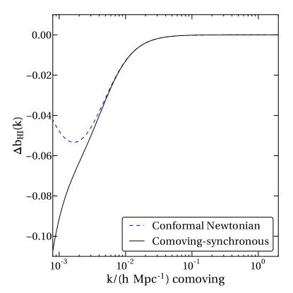
Figure 7: The change in the Hi bias arising from the velocity and potential terms in the radiative transfer. The solid and dashed lines show the conformal-Newtonian (66) and comoving-synchronous expressions respectively. The effects are extremely minor as anticipated.

It may be more natural to think of the bias on large scales in another gauge – it is more plausible, in particular, to imagine that $b_{\mathrm{HI,u}}$ and $b_{j}$ are scale-invariant in the comoving-synchronous than in the conformal-Newtonian gauge Jeong12 . (Ultimately one ought to derive gauge-invariant observables, but for the reasons outlined in the conclusions, that is beyond the scope of the current work.) The gauge transformation consists of a small coordinate transformation $(t,\mathbf{x})\to(t+T,\mathbf{x}+\mathbf{X})$; to reach the comoving-synchronous gauge one uses the freedom to eliminate the peculiar velocities in the coordinate frame. Following this through for any quantity $Z$, assuming $Z_{0}\propto a^{-q}$, one finds that

$$\delta^{N}_{Z}=\delta^{S}_{Z}-2q\phi/3\textrm{,}$$ (67)

where superscript $N$ and $S$ stand for perturbations in conformal-Newtonian and comoving-synchronous gauges respectively. Equation (67) can be used to transform the conformal-Newtonian expression (65) into the synchronous equivalent, giving

$$\hskip 1.42262pt\tilde{\delta}_{n_{\mathrm{HI}}}^{S}=\frac{\hskip 1.42262pt\tilde{\delta}_{n_{\mathrm{HI}},\mathrm{u}}^{S}+\beta_{\phi}\phi-\left[\hskip 1.42262pt\tilde{\delta}_{j}^{S}+\beta_{\phi}\phi+\frac{2}{3}(\beta_{\mathrm{HI}}q_{\mathrm{HI}}-q_{j,\mathrm{eff}})\phi\right]S(k)}{1-\beta_{\mathrm{HI}}S(k)}\textrm{.}$$ (68)

Then, in the synchronous gauge, we have

$$\Delta b_{\mathrm{HI}}^{S}=\frac{-3a^{2}H^{2}}{2c^{2}k^{2}}\frac{\beta_{\phi}-\left[\beta_{\phi}+\frac{2}{3}(\beta_{\mathrm{HI}}q_{\mathrm{HI}}-q_{j,\mathrm{eff}})\right]S(k)}{1-\beta_{\mathrm{HI}}S(k)}\textrm{,}$$ (69)

where $\Delta b_{\mathrm{HI}}^{S}\equiv\Delta\hskip 1.42262pt\tilde{\delta}^{S}_{n_{\mathrm{HI}}}/\hskip 1.42262pt\tilde{\delta}^{S}_{\rho}$, and the result has been obtained using the relation between Newtonian potential and synchronous-gauge density,

$$\phi=\frac{-3a^{2}H^{2}}{2c^{2}k^{2}}\hskip 1.42262pt\tilde{\delta}^{S}\textrm{.}$$ (70)

To gain a quantitative picture we must estimate $q_{\mathrm{HI}}$ and $q_{j}$. Note that for any quantity $Y$ composed of a linear sum of components, $Y=\sum_{i}Y_{i}$, one has

$$q_{Y} =\frac{\mathrm{d}\ln Y}{\mathrm{d}\ln a}=\frac{1}{Y}\sum_{i}\frac{\mathrm{d}Y_{i}}{\mathrm{d}\ln a}=\sum_{i}\beta_{i}q_{Y_{i}}$$ (71)

where $\beta_{i}=Y_{i}/Y$. It therefore follows from using the background equilibrium (27) that

$$q_{j} \approx\left[\beta_{\mathrm{HI}}(1-\beta_{r})+\beta_{\mathrm{clump}}\right]q_{\mathrm{HI}}-\frac{3}{2}\left[\beta_{z}+\beta_{V}\right]\approx 2.7\textrm{;}$$

$$q_{j,\mathrm{eff}} \approx(1-\beta_{\mathrm{HI}}\beta_{\mathrm{r}})q_{j}+(\beta_{\mathrm{HI}}\beta_{\mathrm{r}}-\beta_{\mathrm{clump}})q_{\mathrm{HI}}\approx 2.3\textrm{.}$$ (72)

where I have used $\mathrm{d}\ln H/\mathrm{d}\ln a\approx-3/2$ and $q_{\mathrm{HI}}\simeq 4.3$, the latter from Ref. Rudie13MFP .

Adopting these estimates, equation (69) is plotted as a solid line in Figure 7. The changes are larger than in the Newtonian gauge but still small. It is worth noting that the synchronous gauge bias as derived above describes a different universe – it is not, in fact, related by a gauge transformation to the Newtonian case. This follows because I have formulated both descriptions assuming a constant large-scale bias as an input distribution; this assumption implies something physically different in the two different gauges. As previously stated, it is probably a more appropriate assumption in the synchronous than in the Newtonian gauge.

This, however, is a tangential question because the gravitational and Doppler effects are tiny in both gauges. The original decision to drop these terms is therefore shown to be strongly justified.

Appendix B An estimate of $b_{\mathrm{HI,u}}$

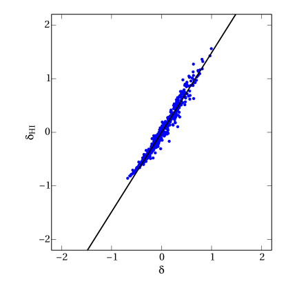
Figure 8: The relationship between Hi overdensity and total matter overdensity in the IGM; each point represents the values averaged in a cube of side length $6\,\mathrm{Mpc}$ comoving at $z=2.3$. This derives from a simulation with uniform UV background. There is a very near-linear relationship between the two quantities, allowing the measurement of the slope (solid line), $b_{\mathrm{HI,u}}\approx 1.5$, which is a parameter entering the main calculation.

To complete the calculation in the main text it was necessary to specify a value of the bias $b_{\mathrm{HI,u}}$ of Hi in the absence of inhomogeneous radiative effects. One can estimate this from the photoionization equilibrium equations for a uniform field, coupled with a description of the temperature-density relation for the averaged IGM. Specifically, the uniform ionization equilibrium in the limit that only a trace of neutral Hi survives specifies 2006agna.book…..O that

$$n_{\mathrm{HI}}\propto\frac{\alpha(T)\,\rho^{2}}{\Gamma_{0}}\textrm{,}$$ (73)

where I have assumed the local electron and proton densities are both proportional to the cosmic density $\rho$. Next write the equation-of-state $T\propto\rho^{\gamma-1}$ and approximate Black81clouds $\alpha(T)\propto T^{-0.7}$; expanding both $\rho$ and $n_{\mathrm{HI}}$ in terms of their background values and perturbations, one obtains

$$b_{\mathrm{HI,u}}=\frac{\delta_{n_{\mathrm{HI}},\mathrm{u}}}{\delta_{\rho}}=2-0.7(\gamma-1)\textrm{.}$$ (74)

For a value HuiGnedin97_IGM_EoS $\gamma=1.6$, this gives an estimate of $b_{\mathrm{HI,u}}\simeq 1.6$.

However, there is a slight inconsistency in the derivation above. The recombination rate actually depends on the strictly local value of the electron and proton densities, not on any linear-theory average on large scales. Depending on how small-scale clustering reflects large-scale density inhomogeneities, the assumption that the local density scales with the environmental density may fail. I therefore also estimated $b_{\mathrm{HI,u}}$ directly from a cosmological simulation with $256^{3}$ dark matter and $256^{3}$ gas particles in a $50\,\mathrm{Mpc}$-side box. The code Gasoline 2004NewA….9..137W implements gravity, hydrodynamics, star formation feedback (which is likely of minor importance here) and a uniform UV field, the values for which I adopted from Ref. HM12 . Much more careful work has been performed in simulating the forest by other authors McDonald00 ; McDonald03 ; Viel_CosmoPars_Lya_2006 but they quote statistics on the flux field, which is related to the Hi field by a non-linear transformation and therefore does not directly tell us $b_{\mathrm{HI,u}}$.

Taking the output at $z=2.3$, I interpolated the gas and dark matter particles back onto a $256^{3}$ grid to obtain two 3D density maps, the first of Hi and the second of total mass density with $\sim 0.2\,\mathrm{Mpc}$ resolution. To study the behaviour of the intergalactic medium, I flagged all cells with dark matter density less than ten times the cosmic mean. Only the flagged cells were subsequently used to produce a degraded map with $8^{3}$ super-cells, in which the mean dark matter and Hi density of the flagged sub-cells was recorded.

This allows us to see the large-scale relationship between IGM overdensity and Hi (Figure 8). Each point represents an IGM super-cell; the two axes correspond to dimensionless total mass overdensity and Hi overdensity in the IGM, expressed as a fraction according to equation (1). The plots show a very near-linear relationship between the total overdensity and the Hi overdensity as expected. The slope of the line gives the bias, which is found to be $b_{\mathrm{HI,u}}=1.48\approx 1.5$. This is in fair agreement with the analytic estimate of $1.6$ given above, given the multitude of uncertainties.

I tested that this result is reasonably insensitive to the size of the super-cells and the IGM threshold density. Repeating the exercise with the IGM threshold at $\delta=5$, for instance, gives $b_{\mathrm{HI,u}}=1.45$; with the original threshold but $16^{3}$ supercells, I retrieve $b_{\mathrm{HI,u}}=1.43$, although the non-linearity in the relation starts to become more prominent (as we are probing smaller scales) so the fit is less meaningful. For the illustrative purposes of this paper, adopting $b_{\mathrm{HI,u}}=1.5$ seems to pin down the large-scale relationship to a sufficient accuracy.

References

- (1) M. Rauch, ARA&A 36, 267 (1998), eprint astro-ph/9806286.
- (2) R. H. Becker, X. Fan, R. L. White, M. A. Strauss, V. K. Narayanan, R. H. Lupton, J. E. Gunn, J. Annis, N. A. Bahcall, J. Brinkmann, et al., AJ 122, 2850 (Dec. 2001), eprint astro-ph/0108097.
- (3) X. Fan, V. K. Narayanan, M. A. Strauss, R. L. White, R. H. Becker, L. Pentericci, and H.-W. Rix, AJ 123, 1247 (Mar. 2002), eprint astro-ph/0111184.
- (4) X. Fan, C. L. Carilli, and B. Keating, ARA&A 44, 415 (Sep. 2006), eprint astro-ph/0602375.
- (5) R. A. C. Croft, D. H. Weinberg, M. Bolte, S. Burles, L. Hernquist, N. Katz, D. Kirkman, and D. Tytler, ApJ 581, 20 (Dec. 2002), eprint astro-ph/0012324.
- (6) P. McDonald, ApJ 585, 34 (Mar. 2003), eprint astro-ph/0108064.
- (7) A. Slosar, A. Font-Ribera, M. M. Pieri, J. Rich, J.-M. Le Goff, É. Aubourg, J. Brinkmann, N. Busca, B. Carithers, R. Charlassier, et al., JCAP 9, 1, 001 (Sep. 2011), eprint 1104.5244.
- (8) M. Viel, J. Lesgourgues, M. G. Haehnelt, S. Matarrese, and A. Riotto, Phys. Rev. D 71(6), 063534, 063534 (Mar. 2005), eprint astro-ph/0501562.
- (9) M. Viel, G. D. Becker, J. S. Bolton, M. G. Haehnelt, M. Rauch, and W. L. W. Sargent, Physical Review Letters 100(4), 041304, 041304 (Feb. 2008), eprint 0709.0131.
- (10) A. Boyarsky, J. Lesgourgues, O. Ruchayskiy, and M. Viel, JCAP 5, 12, 012 (May 2009), eprint 0812.0010.
- (11) A. Slosar, S. Ho, M. White, and T. Louis, JCAP 10, 19, 019 (Oct. 2009), eprint 0906.2414.
- (12) A. Slosar, V. Iršič, D. Kirkby, S. Bailey, N. G. Busca, T. Delubac, J. Rich, É. Aubourg, J. E. Bautista, V. Bhardwaj, et al., JCAP 4, 26, 026 (Apr. 2013), eprint 1301.3459.
- (13) A. Font-Ribera, D. Kirkby, N. Busca, J. Miralda-Escudé, N. P. Ross, A. Slosar, É. Aubourg, S. Bailey, V. Bhardwaj, J. Bautista, et al., JCAP, submitted (Nov. 2013), eprint 1311.1767.
- (14) G. D. Becker, M. Rauch, and W. L. W. Sargent, ApJ 662, 72 (Jun. 2007), eprint astro-ph/0607633.
- (15) J. S. Bolton, M. Viel, T.-S. Kim, M. G. Haehnelt, and R. F. Carswell, MNRAS 386, 1131 (May 2008), eprint 0711.2064.
- (16) G. D. Becker, J. S. Bolton, M. G. Haehnelt, and W. L. W. Sargent, MNRAS 410, 1096 (Jan. 2011), eprint 1008.2622.
- (17) R. A. C. Croft, D. H. Weinberg, N. Katz, and L. Hernquist, ApJ 495, 44 (Mar. 1998), eprint astro-ph/9708018.
- (18) P. McDonald, J. Miralda-Escudé, M. Rauch, W. L. W. Sargent, T. A. Barlow, R. Cen, and J. P. Ostriker, ApJ 543, 1 (Nov. 2000), eprint astro-ph/9911196.
- (19) J. S. Bolton, G. D. Becker, M. G. Haehnelt, and M. Viel, MNRAS 438, 2499 (Mar. 2014), eprint 1308.4411.
- (20) C.-A. Faucher-Giguère, A. Lidz, M. Zaldarriaga, and L. Hernquist, ApJ 703, 1416 (Oct. 2009), eprint 0901.4554.
- (21) F. Haardt and P. Madau, ApJ 746, 125, 125 (Feb. 2012), eprint 1105.2039.
- (22) A. Maselli and A. Ferrara, MNRAS 364, 1429 (Dec. 2005), eprint astro-ph/0510258.
- (23) L. Zuo, MNRAS 258, 36 (Sep. 1992).
- (24) J. A. Kollmeier, D. H. Weinberg, R. Davé, and N. Katz, ApJ 594, 75 (Sep. 2003), eprint astro-ph/0209563.
- (25) A. Meiksin and M. White, MNRAS 350, 1107 (May 2004), eprint astro-ph/0307289.
- (26) J. A. Kollmeier, J. Miralda-Escudé, R. Cen, and J. P. Ostriker, ApJ 638, 52 (Feb. 2006), eprint astro-ph/0503674.
- (27) A. Mesinger and S. Furlanetto, MNRAS 400, 1461 (Dec. 2009), eprint 0906.3020.
- (28) M. White, A. Pope, J. Carlson, K. Heitmann, S. Habib, P. Fasel, D. Daniel, and Z. Lukic, ApJ 713, 383 (Apr. 2010), eprint 0911.5341.
- (29) A. Font-Ribera, E. Arnau, J. Miralda-Escudé, E. Rollinde, J. Brinkmann, J. R. Brownstein, K.-G. Lee, A. D. Myers, N. Palanque-Delabrouille, I. Pâris, et al., JCAP 5, 18, 018 (May 2013), eprint 1303.1937.
- (30) R. A. C. Croft, ApJ 610, 642 (Aug. 2004), eprint astro-ph/0310890.
- (31) P. McDonald, U. Seljak, R. Cen, P. Bode, and J. P. Ostriker, MNRAS 360, 1471 (Jul. 2005), eprint astro-ph/0407378.
- (32) M. McQuinn, L. Hernquist, A. Lidz, and M. Zaldarriaga, MNRAS 415, 977 (Jul. 2011), eprint 1010.5250.
- (33) G. C. Rudie, C. C. Steidel, A. E. Shapley, and M. Pettini, ApJ 769, 146, 146 (Jun. 2013), eprint 1304.6719.
- (34) K. S. Dawson, D. J. Schlegel, C. P. Ahn, S. F. Anderson, É. Aubourg, S. Bailey, R. H. Barkhouser, J. E. Bautista, A. Beifiori, A. A. Berlind, et al., AJ 145, 10, 10 (Jan. 2013), eprint 1208.0022.
- (35) N. G. Busca, T. Delubac, J. Rich, S. Bailey, A. Font-Ribera, D. Kirkby, J.-M. Le Goff, M. M. Pieri, A. Slosar, É. Aubourg, et al., A&A 552, A96, A96 (Apr. 2013), eprint 1211.2616.
- (36) M. McQuinn, S. P. Oh, and C.-A. Faucher-Giguère, ApJ 743, 82, 82 (Dec. 2011), eprint 1101.1964.
- (37) J. Zhang, L. Hui, and Z. Haiman, MNRAS 375, 324 (Feb. 2007), eprint astro-ph/0607628.
- (38) Planck Collaboration, P. A. R. Ade, N. Aghanim, C. Armitage-Caplan, M. Arnaud, M. Ashdown, F. Atrio-Barandela, J. Aumont, C. Baccigalupi, A. J. Banday, et al., A&A, submitted (Mar. 2013), eprint 1303.5076.
- (39) F. Haardt and P. Madau, ApJ 461, 20 (Apr. 1996).
- (40) J. X. Prochaska, P. Madau, J. M. O’Meara, and M. Fumagalli, MNRAS 438, 476 (Feb. 2014), eprint 1310.0052.
- (41) A. Pontzen, F. Governato, M. Pettini, C. M. Booth, G. Stinson, J. Wadsley, A. Brooks, T. Quinn, and M. Haehnelt, MNRAS, accepted (2008).
- (42) J. H. Black, MNRAS 197, 553 (Nov. 1981).
- (43) A. Loeb and S. Furlanetto, The First Galaxies in the Universe, Princeton Series in Astrophysics (Princeton University Press, 2013), ISBN 9781400845606.
- (44) K. Lai, A. Lidz, L. Hernquist, and M. Zaldarriaga, ApJ 644, 61 (Jun. 2006), eprint astro-ph/0510841.
- (45) J. S. Bolton, M. G. Haehnelt, M. Viel, and R. F. Carswell, MNRAS 366, 1378 (Mar. 2006), eprint astro-ph/0508201.
- (46) S. R. Furlanetto, ApJ 703, 702 (Sep. 2009), eprint 0812.3411.
- (47) L. Hui and N. Y. Gnedin, MNRAS 292, 27 (Nov. 1997), eprint astro-ph/9612232.
- (48) C. Bonvin and R. Durrer, Phys. Rev. D 84(6), 063505, 063505 (Sep. 2011), eprint 1105.5280.
- (49) S. M. Croom, B. J. Boyle, T. Shanks, R. J. Smith, L. Miller, P. J. Outram, N. S. Loaring, F. Hoyle, and J. da Ângela, MNRAS 356, 415 (Jan. 2005), eprint astro-ph/0409314.
- (50) M. White, A. D. Myers, N. P. Ross, D. J. Schlegel, J. F. Hennawi, Y. Shen, I. McGreer, M. A. Strauss, A. S. Bolton, J. Bovy, et al., MNRAS 424, 933 (Aug. 2012), eprint 1203.5306.
- (51) K. L. Adelberger, C. C. Steidel, M. Pettini, A. E. Shapley, N. A. Reddy, and D. K. Erb, ApJ 619, 697 (Feb. 2005), eprint astro-ph/0410165.
- (52) N. A. Reddy and C. C. Steidel, ApJ 692, 778 (Feb. 2009), eprint 0810.2788.
- (53) S. Cole and N. Kaiser, MNRAS 237, 1127 (Apr. 1989).
- (54) A. Pontzen, R. Roskar, G. Stinson, and R. Woods, pynbody: N-Body/SPH analysis for python (May 2013), astrophysics Source Code Library, eprint ascl:1305.002.
- (55) B. P. Moster, T. Naab, and S. D. M. White, MNRAS 428, 3121 (Feb. 2013), eprint 1205.5807.
- (56) P. F. Hopkins, G. T. Richards, and L. Hernquist, ApJ 654, 731 (Jan. 2007), eprint astro-ph/0605678.
- (57) N. P. Ross, I. D. McGreer, M. White, G. T. Richards, A. D. Myers, N. Palanque-Delabrouille, M. A. Strauss, S. F. Anderson, Y. Shen, W. N. Brandt, et al., ApJ 773, 14, 14 (Aug. 2013), eprint 1210.6389.
- (58) A. Lewis, A. Challinor, and A. Lasenby, Astrophys. J. 538, 473 (2000), eprint astro-ph/9911177.
- (59) A. Font-Ribera, J. Miralda-Escudé, E. Arnau, B. Carithers, K.-G. Lee, P. Noterdaeme, I. Pâris, P. Petitjean, J. Rich, E. Rollinde, et al., JCAP 11, 59, 059 (Nov. 2012), eprint 1209.4596.
- (60) P. McDonald, U. Seljak, S. Burles, D. J. Schlegel, D. H. Weinberg, R. Cen, D. Shih, J. Schaye, D. P. Schneider, N. A. Bahcall, et al., ApJS 163, 80 (Mar. 2006), eprint astro-ph/0405013.
- (61) L. Anderson, E. Aubourg, S. Bailey, F. Beutler, A. S. Bolton, J. Brinkmann, J. R. Brownstein, C.-H. Chuang, A. J. Cuesta, K. S. Dawson, et al., MNRAS 439, 83 (Mar. 2014), eprint 1303.4666.
- (62) N. Kaiser, MNRAS 227, 1 (Jul. 1987).
- (63) J. A. Peacock, Cosmological physics (Cambridge University Press, Cambridge, UK, 1999).
- (64) J. R. Pritchard and A. Loeb, Reports on Progress in Physics 75(8), 086901, 086901 (Aug. 2012), eprint 1109.6012.
- (65) S. R. Furlanetto, M. Zaldarriaga, and L. Hernquist, ApJ 613, 1 (Sep. 2004), eprint astro-ph/0403697.
- (66) A. D’Aloisio, J. Zhang, P. R. Shapiro, and Y. Mao, MNRAS 433, 2900 (Aug. 2013), eprint 1304.6411.
- (67) Y. Mao, A. D’Aloisio, J. Zhang, and P. R. Shapiro, Phys. Rev. D 88(8), 081303, 081303 (Oct. 2013), eprint 1305.0313.
- (68) V. F. Mukhanov, H. A. Feldman, and R. H. Brandenberger, Phys. Rep. 215, 203 (Jun. 1992).
- (69) D. Jeong, F. Schmidt, and C. M. Hirata, Phys. Rev. D 85(2), 023504, 023504 (Jan. 2012), eprint 1107.5427.
- (70) D. E. Osterbrock and G. J. Ferland, Astrophysics of gaseous nebulae and active galactic nuclei (Sausalito, CA: University Science Books, 2006).
- (71) J. W. Wadsley, J. Stadel, and T. Quinn, New Astronomy 9, 137 (Feb. 2004).
- (72) M. Viel and M. G. Haehnelt, MNRAS 365, 231 (Jan. 2006), eprint astro-ph/0508177.