Modeling phase transition and metastable phases

Abstract

We propose a model that describes phase transition including metastable phases present in the van der Waals Equation of State (EoS). We introduce a dynamical system that is able to depict the mass transfer between two phases, for which equilibrium states are both metastable and stable states, including mixtures. The dynamical system is then used as a relaxation source term in a isothermal two-phase model. We use a Finite volume scheme (FV) that treats the convective part and the source term in a fractional step way. Numerical results illustrate the ability of the model to capture phase transition and metastable states.

1 Introduction

Metastable liquids are liquid states where the temperature is higher than the ebullition temperature. Such states are very unstable and a very small perturbation brings out a bubble of vapor inside the liquid. Such phenomenon can appear at saturated temperature (or at saturated pressure for metastable vapor) for instance inside a nozzle such as fuel injector or cooling circuit of water pressurized reactor. In the last decades considerable research has been devoted to the modeling of two-phase flows with phase transition. However the exact expressions of the transfer mass term are usually unknown (see drew83 ). In particular, to our knowledge, there is very few literature about the transfer term able to depict metastable states. In saurel08 and zein10 the authors consider a 6 equation model where relaxation to equilibrium is achieved by chemical and pressure relaxation terms whose kinetics are considered infinitely fast.

We intend here to provide a new model able to depict phase transition and metastable states with non-infinite relaxation speed. It is based on the use of the van der Waals EOS, that is well-known to depict stable and metastable states below the critical temperature. However this EOS is not valid in the so-called spinodal zone where the pressure is a decreasing function of the density. This leads to instabilities and computational failure and the pressure has to be corrected using the Maxwell equal area rule construction to recover a constant pressure. But such a correction removes the metastable regions. We propose transfer terms obtained through an optimization problem of the Helmholtz free energy of the two-phase system. For sake of simplicity we assume the system to be isothermal. We obtained a dynamical system that is able to depict mass transfer including metastable states and that dissipates the total Helmholtz free energy. The equilibria of the dynamical system are both stable and metastable states and mixture states that satisfies the pressures and chemical potentials equalities. This dynamical system is used as transfer term in a isothermal two-phase model in the spirit of guillard05 and chalons09 . We use a classical FV scheme that treats the convective and the source terms in a splitting approach.

Section 2 is devoted to the thermodynamics of binary mixture and presents the major properties of the van der Waals EoS. Section 3 is devoted to the construction of the dynamical system based on results of the previous Section. In particular we show that metastable states are attractors of the dynamical system. In Section 4 we briefly present the splitting FV scheme we use and give numerical results where metastable vapor appears.

2 Thermodynamics and van der Waals Equation of State

In this Section we first recall the thermodynamics theory for a single isothermal fluid and introduce the different potentials of the van der Waals EoS, then we state the mathematical framework for the thermodynamics of immiscible binary mixtures.

2.1 Thermodynamics of a single phase

Consider a single fluid of mass $M>0$ occupying a volume $V>0$. At constant temperature if the fluid is homogeneous and at rest, its behavior is entirely described by the Helmholtz free energy function $E(M,V)$ which belongs to $C^{2}(\mathbb{R}_{+}\times\mathbb{R}_{+})$ and is positively homogeneous of degree 1 (PH1). Thus, at fixed volume $V$, one can introduce the specific Helmholtz free energy $f$ and the specific energy $e$ that are functions of the density $\rho=M/V$

$$f(\rho)=E(\rho,1),\qquad\rho e(\rho)=E(\rho,1).$$ (1)

We introduce also the pressure $p$ and the chemical potential $\mu$ that are partial derivatives of the free energy $E$, respectively with respect to $V$ and $\rho$. By homogeneity, one can write them as functions of $\rho$ solely:

$$p(\rho)=-\partial_{V}E(\rho,1),\qquad\mu(\rho)=\partial_{M}E(\rho,1).$$ (2)

Again thanks to the homogeneity of the energy function, one has

$$f(\rho)=\rho\mu(\rho)-p(\rho),\qquad f^{\prime}(\rho)=\mu(\rho).$$ (3)

Stable pure phases are characterized by a convex energy function, which leads to a nondecreasing pressure law. We consider a classical example of a fluid that may experience phase transitions, namely the van der Waals monoatomic fluid. At fixed temperature $T$ its Helmholtz free energy is given by

$$E(M,V)=-\dfrac{aM^{2}}{V}+RT\left(M\log\dfrac{M}{V-Mb}-M\right),$$ (4)

where $R$ stands for the perfect gas constant and $a$ and $b$ are positive constants, $a$ accounts for binary interactions and $b$ is the covolume. Below a critical temperature $T_{C}$ the pressure law is no longer monotone (see fig. 1): in a region called the spinodal zone, the pressure decreases with respect to the density, thus leading to instable states. In that region the isotherm have to be replaced by the maxwell area rule in order to recover that phase transition happens at constant pressure and chemical potential. However this construction removes admissible regions where the pressure law is still nondecreasing. Such regions are called the metastable regions (blue regions in fig. 1). We consider in the following the dimensionless equation of state and the associated potentials for which $R=8/3$, $a=3$ and $b=1/3$, for which $T_{C}=1$.

[scale=.35]dome.pdf

Figure 1: Phase diagram for the van der Waals EoS in the $(p,\rho)$ plan. The red curve stands for an isotherm below the critical temperature $T_{C}$, the point $C$ being the critical point. The orange zone is called spinodal zone, it corresponds to unstable states. In that area the isotherm has to be replaced by an horizontal segment that coincides with the isobaric line at constant pressure $p^{*}$.

2.2 Equilibrium of a two-phase mixture

We consider now two immiscible phases of a same pure fluid of total mass $M$ and volume $V$. Each phase $i=1,2,$ is depicted by its mass $M_{i}\geq 0$ and its volume $V_{i}\geq 0$. We assume that both phases are characterized by the same van der Waals extensive Helmholtz free energy $E$ function of $M_{i}$ and $V_{i}$, given by (4). By the conservation of mass, the mass of the binary system is $M=M_{1}+M_{2}$ and immiscibility implies $V=V_{1}+V_{2}$.

According to the second principle of thermodynamics (see Gibbs ), for fixed mass $M$ and volume $V$ the stable equilibrium states of the system are the solutions to the constrained optimization problem

$$\inf\{E(M_{1},V_{1})+E(M_{2},V_{2})|\;V_{1}+V_{2}=V,\;M_{1}+M_{2}=M\},$$

which can be rewritten using (1) in term of the specific Helmholtz free energy at fixed density $\rho$:

$$\inf\{\alpha_{1}f(\rho_{1})+\alpha_{2}f(\rho_{2})|\;\alpha_{1}+\alpha_{2}=1,\;\alpha_{1}\rho_{1}+\alpha_{2}\rho_{2}=\rho\},$$ (5)

where $\alpha_{i}=V_{i}/V\in[0,1]$ denotes the volume fraction and $\rho_{i}=M_{i}/V_{i}$ is the density of the phase $i=1,2$. In the sequel the fractions $\alpha_{i}$ are written as functions of $\rho,\rho_{1}$ and $\rho_{2}$ such that $\alpha_{1}(\rho,\rho_{1},\rho_{2})=(\rho-\rho_{2})/(\rho_{1}-\rho_{2})$ and $\alpha_{2}(\rho,\rho_{1},\rho_{2})=1-\alpha_{1}(\rho,\rho_{1},\rho_{2})$.

Note that $\alpha_{1}$ and $\alpha_{2}$ are simultaneously non zero if and only if $\rho_{1}\neq\rho_{2}$. In that case we shall always assume without loss of generality that $\rho_{1}<\rho_{2}$ and $\rho\in[\rho_{1},\rho_{2}]$. The total Helmholtz free energy $F:\mathbb{R}_{+}^{3}\to\mathbb{R}$ of the binary system is given by

$$F(\rho,\rho_{1},\rho_{2})=\alpha_{1}(\rho,\rho_{1},\rho_{2})f(\rho_{1})+\alpha_{2}(\rho,\rho_{1},\rho_{2})f(\rho_{2}).$$ (6)

Depending on the saturation of the volume fractions, one can characterize the equilibria of the optimization problem (5).

Proposition 1

1. Pure states: if $\alpha_{1}=0$ (resp. $\alpha_{2}=0$) then only the phase $2$ (resp. 1) is stable.

2. Mixture: if $\alpha_{1}\alpha_{2}\neq 0$, then the equilibrium state is characterized by one of the following equivalent properties

   1. equality of the chemical potentials and the pressures

      $$\mu(\rho_{1})=\mu(\rho_{2})=\mu^{*},\quad p(\rho_{1})=p(\rho_{2})=p^{*},$$ (7)

   2. Maxwell area rule on the chemical potential

      $$\int_{0}^{1}\mu(\rho_{2}+t(\rho_{1}-\rho_{2}))dt=\mu(\rho_{1})=\mu(\rho_{2})=\mu^{*},$$ (8)

   3. the difference of the energies reads

      $$f(\rho_{2})-f(\rho_{1})=\mu(\rho_{1})(\rho_{2}-\rho_{1})=\mu(\rho_{2})(\rho_{2}-\rho_{1}).$$ (9)

The densities such that (7), (8) or (9) hold are denoted $\rho_{1}^{*}$ and $\rho_{2}^{*}$, see fig. 1.

The most important consequence of this result is that in the metastable zones there are two possible equilibrium states corresponding to a pure metastable state and a stable mixture state. Hence the EoS at equilibrium is not single-valued. The difference between stable and metastable states lies in their dynamical behaviour with respect to perturbations, see Landau .

3 Dynamical system and phase transition

We turn now to the study of dynamical stability of equilibrium states. First we address the homogenous case, introducing a dynamical system for which the equilibria are both stable and metastable states as well as states in the spinodal area such that (7)-(8) are satisfied. Next the dynamical system is plugged as a relaxation source terms in a isothermal two-fluid model. Some properties of the full model are given: hyperbolicity, existence of a energy function that decreases in time.

3.1 Dynamical system

Assuming that $\rho$, $\rho_{1}$ and $\rho_{2}$ are only time-dependent, we introduce the following dynamical system, which derives from the optimality conditions of Proposition 1:

$$\dot{\rho} = 0,$$

$$\dot{\rho}_{1} = -(\rho-\rho_{1})(\rho-\rho_{2})\left(\rho_{2}(\mu(\rho_{2})-\mu(\rho_{1}))+p(\rho_{1})-p(\rho_{2})\right),$$ (10)

$$\dot{\rho}_{2} = (\rho-\rho_{1})(\rho-\rho_{2})\left(\rho_{1}(\mu(\rho_{1})-\mu(\rho_{2}))-p(\rho_{1})+p(\rho_{2})\right).$$

Straightforward computions show that the total Helmholtz free energy $F$ defined by (6) decreases in time along the solutions of this system. We focus now on the equilibria which can be reached by the model (under the assumption $\rho_{1}<\rho_{2}$).

Theorem 3.1

The equilibria of the system (3.1) are

1. the monophasic states such that $\alpha_{1}=1$ (resp. $\alpha_{1}=0$) that is $\rho=\rho_{1}=\overline{\rho}$ with any $\rho_{2}\neq\overline{\rho}$ (resp. $\rho=\rho_{2}=\overline{\rho}$ with any $\rho_{1}\neq\overline{\rho}$). In that case, if $\rho=\rho_{i}$, $i=1$ or $2$ such that

   1. $\rho\not\in[\rho^{-},\rho^{+}]$, then the equilibrium is an attractor and corresponds to monophasic and metastable states,

   2. $\rho\in[\rho^{-},\rho^{+}]$, then the equilibrium is a repeller and corresponds to states belonging to the spinodal zone (which is non admissible),

2. the unique state such that $0<\alpha_{1}<1$ and the relations (7)-(8) are satisfied.

A remarkable feature of this system is that a perturbation of a pure metastable state involving the other phase leads to a mixture equilibrium state, corresponding to the definition of metastable state Landau .

3.2 The isothermal model

The previous dynamical system (3.1) is now coupled with a modified version of the isothermal two-phase model proposed in chalons09 (see also guillard05 ). The model admits a mixture pressure $\alpha_{1}p(\rho_{1})+\alpha_{2}p(\rho_{2})$ and one velocity $u$ for both phases. It reads

$$\partial_{t}\rho+\partial_{x}(\rho u) =\dfrac{1}{\varepsilon}\dot{\rho}=0,$$ (11)

$$\partial_{t}\rho_{i}+\partial_{x}(\rho_{i}u) =\dfrac{1}{\varepsilon}\dot{\rho_{i}},\qquad i=1,2$$

$$\partial_{t}(\rho u)+\partial_{x}(\rho u^{2}+\alpha_{1}p(\rho_{1})+\alpha_{2}p(\rho_{2})) =0,$$

where the source terms are given by the dynamical system (3.1) and account for mass and mechanical transfer. The parameter $\varepsilon>0$ is a relaxation parameter that represents the relaxation time to reach thermodynamical equilibrium. In order to capture metastable states, we will consider $0<\varepsilon<1$ in computations.

The convective part of the model (11) is hyperbolic with the eigenvalues

$$\lambda_{1}=u-c,\quad,\lambda_{2}=\lambda_{3}=u,\quad\lambda_{4}=u+c,$$ (12)

where the speed of sound is $c=\sqrt{\dfrac{1}{\rho}(\alpha_{1}\rho_{1}p^{\prime}(\rho_{1})+\alpha_{2}\rho_{2}p^{\prime}(\rho_{2}))}$.

Proposition 2

The function $\mathcal{E}(\rho,\rho_{1},\rho_{2},u)=\dfrac{\rho u^{2}}{2}+\alpha_{1}f(\rho_{1})+\alpha_{2}f(\rho_{2})$, satisfies the following equation

$$\partial_{t}(\mathcal{E})+\partial_{x}(u(\mathcal{E}+\alpha_{1}p(\rho_{1})+\alpha_{2}p(\rho_{2}))=(\partial_{\rho_{1}}F)\dot{\rho_{1}}+(\partial_{\rho_{2}}F)\dot{\rho_{2}}\leq 0.$$ (13)

Note that $\mathcal{E}$ is not an entropy of the system since $f$ is a non-convex function of the density.

4 Numerical illustration

We present here numerical results that assess the ability of the model to capture phase transition including metastable states. We use a standard Finite Volume method to approximate the Cauchy problem

$$\partial_{t}W+\partial_{x}F(W)=S(W),\qquad W(0,x)=W_{0}(x),\,x\in\mathbb{R},$$ (14)

where $W=(\rho,\rho_{1},\rho_{2},\rho u)^{T}$, $F(W)=(\rho u,\rho_{1}u,\rho_{2}u,\rho u^{2}+\alpha_{1}p(\rho_{1})+\alpha_{2}p(\rho_{2}))^{T}$, and $S(W)=(0,\dfrac{1}{\varepsilon}\dot{\rho}_{1},\dfrac{1}{\varepsilon}\dot{\rho}_{2},0)^{T}$. We use a fractional step approach. We denote $\Delta t$ the time step and $\Delta x$ the length of the cell $(x_{i-1/2},x_{i+1/2})$ on the regular 1D-mesh. Let $W^{n}$ be the Finite Volume approximation at time $t^{n}=n\Delta t$, $n\in\mathbb{N}$. The first step corresponds to the approximation of the convective part which provides the solution $W^{n,-}$ at time $t^{n,-}$. It is treated by a classical Rusanov scheme. The second step is the approximation of the source terms (relaxation), at this stage we merely use an explicit Euler method.

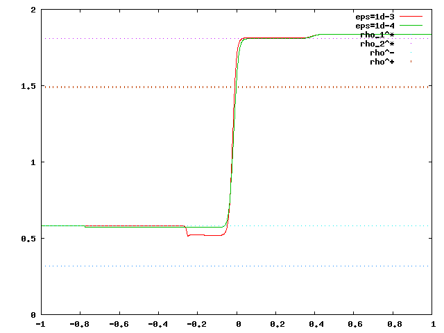
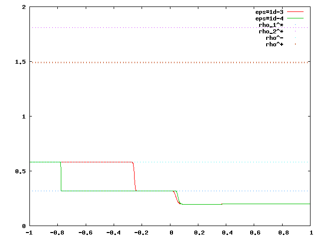
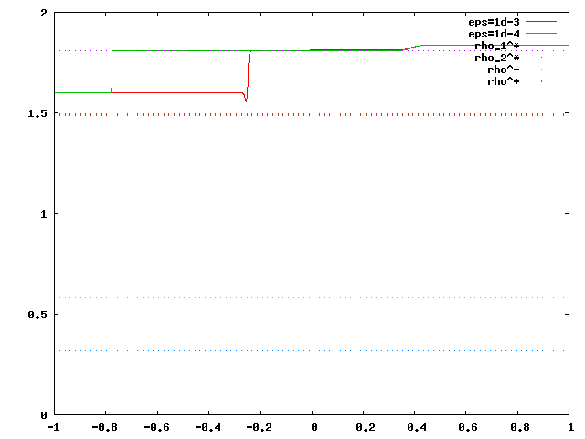
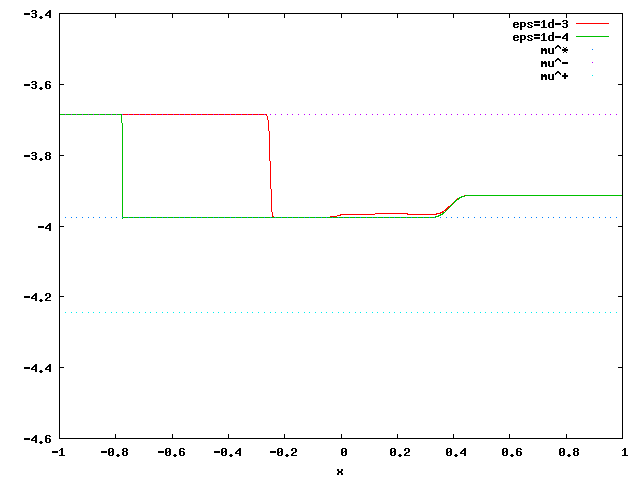
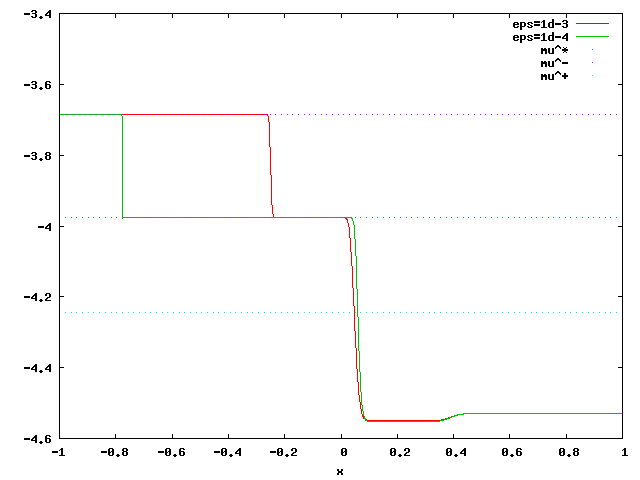
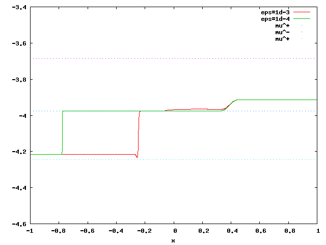
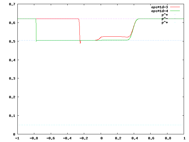
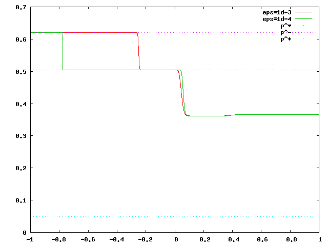
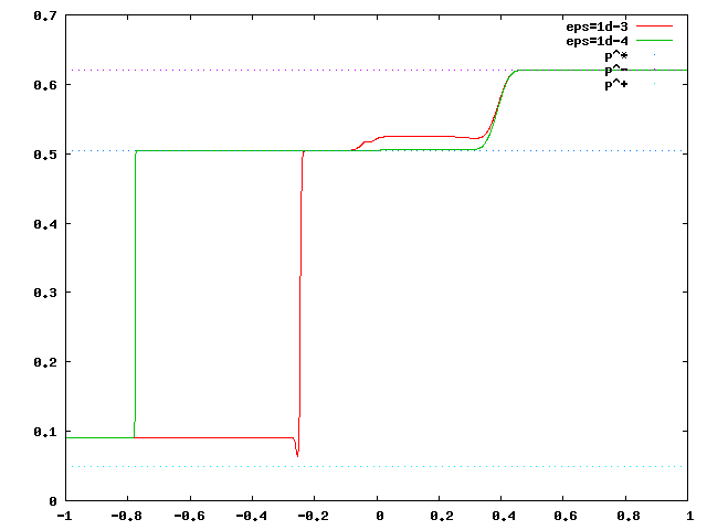
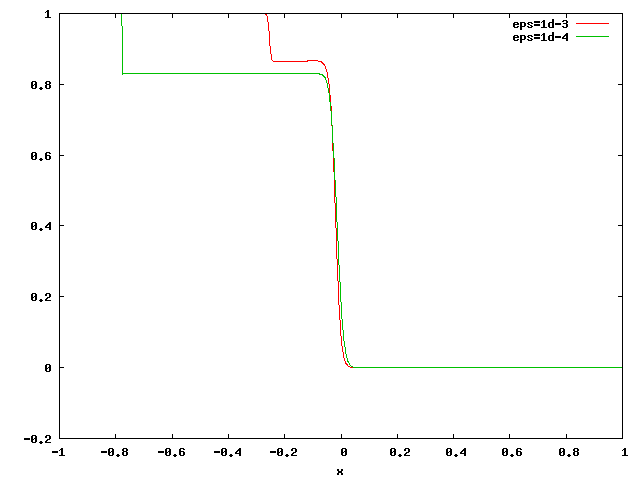
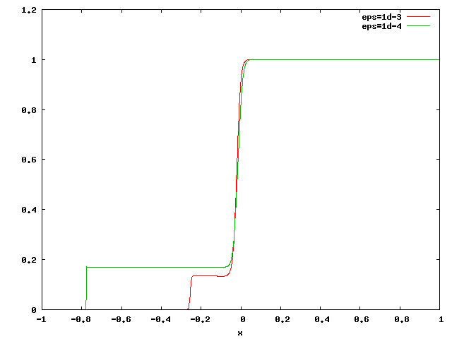
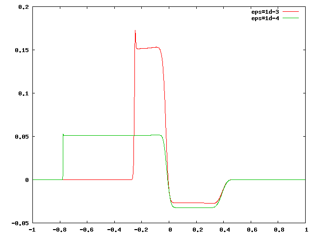
Figure 2: First line, densities: $\rho$, $\rho_{1}$, $\rho_{2}$, second line, chemical potentials: $\mu$, $\mu_{1}$, $\mu_{2}$, third line, pressures: $p$, $p_{1}$, $p_{2}$, last line fractions $\alpha_{1}$, $\alpha_{2}$ and the velocity $u$.

We consider the van der Waals equation at constant temperature $T=0.85$. The extrema of the isotherm curve are $\rho^{-}=0.581079$ and $\rho^{+}=1.488804$. The Maxwell construction on the chemical potential defines the densities $\rho_{1}^{*}=0.319729$ and $\rho_{2}^{*}=1.807140$ such that $\mu(\rho_{1}^{*})=\mu(\rho_{2}^{*})=3.977178$ and $p(\rho_{1}^{*})=p(\rho_{2}^{*})=0.504492$. If the Riemann problem consists in an initial constant pressure and constant chemical potential state, the numerical scheme preserves this state exactly as it is expected. Another test case consists in an initial constant pressure state which is subjected to a disequilibrium in chemical potential. The initial data are $\rho_{L}=\rho_{1,L}=\rho^{-}$, $\rho_{2,L}=1.6$, $\rho_{R}=\rho_{2,R}=1.837840$, $\rho_{1,R}=0.2$ and $u_{L}=u_{R}=0$. The discontinuity is applied at $x=0$ in the domain $[-1,1]$. The mesh contains with 2000 cells and the time of computation is $t=0.2$. Note that $\rho_{2,L}$ belongs to the metastable liquid region and $\rho_{2,R}$ belongs to the pure liquid region such that $p(\rho_{2,R})=p(\rho^{-})=p(\rho_{1,L})$ and $\rho_{1,R}$ belongs to the pure gaseous region. Fig. 2 presents the results for $\varepsilon=10^{-3}$ and $\varepsilon=10^{-4}$. The main feature to notice here is that the relaxation approximation introduces a mixture zone on both sides of the interface, which remains stable. Within this zone, there are variations of the velocity, which remains compressive ($u>0$ for $x<0$, $u<0$ for $x>0$).

5 Conclusion and prospects

The first tests with this model show that it is able to cope with phase transitions with metastable states using a van der Waals EoS. Due to the complexity of the source term, we propose as a first step an explicit treatment of the relaxation term. We aim at providing a semi-implicit scheme in the spirit of GHS04 . Moreover this model is a toy one since it is isothermal. We attend to add the temperature dependance to obtain a fully heat, mass and mechanical transfer model in order to compare our results to the one of saurel08 and zein10 .

Acknowledgement The second author is supported by the project ANR-12-IS01-0004-01 GEONUM.

References

- (1) Ambroso, A., Chalons, C., Coquel, F., Galié, T.: Relaxation and numerical approximation of a two-fluid two-pressure diphasic model. M2AN Math. Model. Numer. Anal. 43(6), 1063–1097 (2009)
- (2) Drew, D.: Mathematical modeling of two-phase flow. Ann. Rev. Fluid Mech. 15, 261–291 (1983)
- (3) Gallouët, T., Hérard, J.M., Seguin, N.: Numerical modeling of two-phase flows using the two-fluid two-pressure approach. Math. Models Methods Appl. Sci. 14(5), 663–700 (2004)
- (4) Gibbs, J.W.: The Collected Works of J. Willard Gibbs, vol I: Thermodynamics. Yale University Press (1948)
- (5) Landau, L., Lifschitz, E.: A Course of theoretical physics, vol 5, Statistical Physics, ch 8. Pergamon Press (1969)
- (6) Murrone, A., Guillard, H.: A five equation reduced model for compressible two phase flow problems. J. Comput. Phys. 202(2), 664–698 (2005)
- (7) Saurel, R., Petitpas, F., Abgrall, R.: Modelling phase transition in metastable liquids: application to cavitating and flashing flows. J.Fluid Mech. 607, 313–350 (2008)
- (8) Zein, A., Hantke, M., Warnecke, G.: Modeling phase transition for compressible two-phase flows applied to metastable liquids. J. Comp. Phys. 229, 1964–2998 (2010)