Bundle-based pruning in the max-plus curse of dimensionality free method

Abstract

Recently a new class of techniques termed the max-plus curse of dimensionality-free methods have been developed to solve nonlinear optimal control problems. In these methods the discretization in state space is avoided by using a max-plus basis expansion of the value function. This requires storing only the coefficients of the basis functions used for representation. However, the number of basis functions grows exponentially with respect to the number of time steps of propagation to the time horizon of the control problem. This so called “curse of complexity” can be managed by applying a pruning procedure which selects the subset of basis functions that contribute most to the approximation of the value function. The pruning procedures described thus far in the literature rely on the solution of a sequence of high dimensional optimization problems which can become computationally expensive.

In this paper we show that if the max-plus basis functions are linear and the region of interest in state space is convex, the pruning problem can be efficiently solved by the bundle method. This approach combining the bundle method and semidefinite formulations is applied to the quantum gate synthesis problem, in which the state space is the special unitary group (which is non-convex). This is based on the observation that the convexification of the unitary group leads to an exact relaxation. The results are studied and validated via examples.

I INTRODUCTION

One general approach to the solution of optimal control problem is the dynamic programming principle, which in the deterministic case leads to a first-order, nonlinear partial differential equation, the Hamilton-Jacobi-Bellman Partial Differential Equation (HJB PDE). Classical numerical methods for solving the HJB PDE, as the finite difference scheme [CL84] or the semi-Lagrangian scheme [Fal87, FF94], are all grid-based and known to suffer from the so called curse of dimensionality, meaning that the number of grid points should grow exponentially with the space dimension.

In recent years, a new class of numerical methods has been developed after the work of Fleming and McEneaney [FM00], see [McE06, AGL08, SGJM10, DM11]. These methods, named max-plus basis methods, exploit the linearity of the associated semigroup in the max-plus algebra. Only the time interval is discretized and at each discretized time step, the value function is approximated by a supremum (or infimum if the objective is minimized) of basis functions. Among several max-plus basis methods, the curse of dimensionality-free method introduced by McEneaney [McE07] is of special interest because of its polynomial growth rate of the computational complexity with the space dimension. It applies to the class of optimal control problems where the Hamiltonian is given or approximated by a pointwise supremum of a finite number of “simpler” Hamiltonians. In particular, such Hamiltonians arise when the control space is discrete, for example in switched systems. However, the number of basis functions is multiplied by the number of simpler Hamiltonians at each propagation. Therefore in the practical implementation, a pruning operation removing at each propagation a certain number of basis functions less useful than others is required to attenuate this so called curse of complexity.

In order to sort the basis functions for the pruning, an importance metric is associated to each basis function. The latter measures the maximal lost caused by removing the corresponding basis function. The smaller the importance metric is, the less useful the basis function is. Hence, the pruning operation consists of sorting the basis functions by their importance metrics and selecting those with largest importance metrics. Hence the attenuation of the curse of complexity in the max-plus curse of dimensionality-free method is reduced to the calculus of importance metrics.

In the previous related works [MDG08, SGJM10, GMQ11], the importance metric is given or approximated as the optimal value of a convex semidefinite program and solved by the package CVX or YALMIP, calling the standard convex optimization solver SEDUMI or SDPT3. At each propagation in the max-plus curse of dimensionality-free method, if the number of basis functions is $m$, then we need to solve $m$ semidefinite programs of size $m$. The complexity of a standard convex optimization solver is polynomial to the program size $m$, in the worst case $O(m^{3.5})$ [BV04]. However, the number of basis functions $m$ is supposed to grow exponentially with respect to the number of propagation steps. Hence, it is necessary to develop a method more efficient than the general-purpose solver for the importance metric calculus when the number of basis functions $m$ is large.

Large-scale convex optimization has received many attentions. The most common approach in the literature is to reduce the complexity of the inversion of the linear equations in the interior point method, either by exploiting the sparsity [SNW12, Chapter 3] or by designing customized algorithms [LV07, KKB07, WHJ09]. A non-interior-point approach is the bundle method [HR00]. In this paper, we first remark that when the basis functions are all linear and the state space is convex, the bundle method can be an alternative algorithm for the calculus of the importance metric. In order to apply the bundle method to the quantum gate synthesis problem [SGJM10] in which the state space is the unitary group, we need to convexify the unitary group. On the other hand, we show that the convexification of the unitary group leads to an exact relaxation. The efficiency of the bundle method is demonstrated via numerical examples, by comparison with the standard package CVX.

The paper is organized as follows. In Section II, we review the general principle of the max-plus curse of dimensionality-free method, extract the importance metric calculus problem and propose Algorithm 1 applying the bundle method. In Section III, we consider the quantum gate synthesis application. In Section IV, we show that the convexification of the unitary group leads to an exact relaxation. In Section V, we present numerical results demonstrating the efficiency of the bundle method.

The notations used in the paper are the following. For $a\in\mathbb{C}$, $\operatorname{Re}(a)$ is the real part of $a$. The space of $n\times n$ complex matrices is denoted by $M_{n}(\mathbb{C})$. For $X\in M_{n}(\mathbb{C})$, $X^{*}$ denotes its conjugate transpose. The space $M_{n}(\mathbb{C})$ is considered as a real Hilbert space endowed with an inner product $\langle\cdot,\cdot\rangle$ given by:

$$\langle X_{1},X_{2}\rangle=\operatorname{Re}(\operatorname{trace}(X_{1}^{*}X_{2})),\enspace\forall X_{1},X_{2}\in M_{n}(\mathbb{C})\enspace.$$

The induced norm of a matrix $X\in M_{n}(\mathbb{C})$ is denoted by $\|X\|$. The space of $n\times n$ positive semidefinite (resp. positive definite) matrices is denoted by $\operatorname{S}_{n}^{+}$ (resp. $\hat{\operatorname{S}}_{n}^{+}$). For two Hermitian matrices $A,B\in M_{n}(\mathbb{C})$, we write $A\succcurlyeq B$ (resp. $A\succ B$) if $A-B\in\operatorname{S}_{n}^{+}$ is (resp. $A-B\in\hat{\operatorname{S}}_{n}^{+}$). For $k\in\mathbb{N}$, we denote by $I_{k}$ the identity matrix of size $k$. We denote by $U(n)$ the group of $n\times n$ unitary matrices and $B(n)$ the set of $n\times n$ matrices of spectral norm less than 1:

$$B(n):=\{X\in M_{n}(\mathbb{C}):XX^{*}\preccurlyeq I_{n}\}\enspace.$$

II MAX-PLUS CURSE OF DIMENSIONALITY FREE METHOD

The main objective of this section is to introduce the pruning problem arising in the max-plus curse of dimensionality free method. For this purpose, we first review briefly the principle of the method in a general framework.

II-A Problem class

Denote by $\mathcal{X}\subset\mathbb{R}^{d}$ the state space and by $\mathcal{U}\subset\mathbb{R}^{m}$ the control space. Let $x\in\mathcal{X}$ and $T\in(0,+\infty]$. Consider the following optimal control problem:

$$V_{T}(x):=\inf_{\mathbf{u}}\int_{0}^{T}\ell(\mathbf{x}(s),\mathbf{u}(s))ds+\phi(\mathbf{x}(T))\enspace,$$

where the state trajectory $\mathbf{x}(\cdot):[0,T)\rightarrow\mathcal{X}$ satisfies the dynamics:

$$\dot{\mathbf{x}}(s)=f(\mathbf{x}(s),\mathbf{u}(s)),\quad\mathbf{x}(0)=x\in\mathcal{X}\enspace.$$

The functions $f:\mathcal{X}\times\mathcal{U}\to\mathbb{R}^{d}$, $\ell:\mathcal{X}\times\mathcal{U}\to\mathbb{R}$ and $\phi:\mathcal{X}\to\mathbb{R}$ represent the dynamics, the running cost and the terminal cost, respectively. The value $V_{\cdot}(\cdot):\mathcal{X}\times(0,T)\rightarrow\mathbb{R}$ gives the optimum of the objective as a function of the initial state $x$ and of the horizon $T$, called value function. In this general framework, we omit the necessary assumptions on the functions $f$, $\ell$ and $\phi$ to guarantee the existence and regularity of the value function. The Hamiltonian associated to the above optimal control problem is:

$$H(x,p)=\sup_{u\in\mathcal{U}}\langle p,f(x,u)\rangle+\ell(x,u),\enspace\forall x,p\in\mathbb{R}^{d}\enspace.$$

The corresponding Hamilton-Jacobi Partial Differential Equation (HJ PDE) is then:

$$\left\{\begin{array}[]{l}\frac{\partial V}{\partial t}(t,x)-H(x,\frac{\partial V}{\partial x}(t,x))=0,\qquad\forall(x,t)\in\mathcal{X}\times(0,T)\enspace,\\ V_{0}(x)=\phi(x),\quad\forall x\in\mathcal{X}\enspace.\end{array}\right.$$ (1)

The Lax-Oleinik semigroup $(S_{t})_{t\geqslant 0}$ associated to the Hamiltonian $H$ is the evolution semigroup of the corresponding HJ PDE (1), i.e.,

$$S_{t}[\phi]=V_{t},\quad\forall t\in(0,T)\enspace.$$

In max-plus basis methods [FM00], we choose a set of basis functions ${\mathcal{B}}=\{\omega_{i}:\mathbb{R}^{d}\rightarrow\mathbb{R}\}_{i\in J}$ and approximate the value function $V_{T}$ by the infimum of a finite number of basis functions. More precisely, we need to determine a subset $I$ and approximate $V_{T}$ as follows:

$$V_{T}(x)\simeq\inf_{i\in I}\omega_{i}(x),\enspace\forall x\in\mathcal{X}\enspace.$$

The max-plus curse of dimensionality free method [McE07] applies to the class of optimal control problems where the Hamiltonian is given or approximated by the supremum of “simpler” Hamiltonians:

$$H(x,p)\simeq\sup_{m\in\mathcal{M}}H^{m}(x,p),\enspace\forall x,p\in\mathbb{R}^{d}\enspace,$$

where $\mathcal{M}$ is a finite index set. The term “simpler” refers to the condition that for all $\omega_{i}\in{\mathcal{B}}$, $t\geqslant 0$ and $m\in\mathcal{M}$, the computation cost of $S_{t}^{m}[\omega_{i}]$ is polynomial to the state dimension $d$. Moreover, we require that $S_{t}^{m}[\omega_{i}]$ is in ${\mathcal{B}}$.

Example II.1

In the original development of the method [McE07], McEneaney considered the switching linear quadratic optimal control problem where the Hamiltonian is given by the supremum of quadratic forms:

$$H(x,p)=\sup_{m\in\mathcal{M}}(A^{m}x)^{\prime}p+\frac{1}{2}x^{\prime}D^{m}x+\frac{1}{2}p^{\prime}\Sigma^{m}p,\enspace\forall x,p\in\mathbb{R}^{d}\enspace.$$

The matrices $\{A^{m},D^{m},\Sigma^{m}:m\in\mathcal{M}\}$ are parameters of the switching system. The set of basis functions ${\mathcal{B}}$ is chosen to be a set of bounded quadratic functions. The optimal control problem corresponding to each $H^{m}$ is a linear quadratic control problem. Then for each quadratic basis function $\omega_{i}\in{\mathcal{B}}$, $S_{t}^{m}[\omega_{i}]$ is still a quadratic function for all $t\geqslant 0$ and $m\in\mathcal{M}$. Besides, the computation requires only the resolution of a Riccati differential equation, thus of cost $O(d^{3})$.

Example II.2

The method finds application in the study of quantum circuit complexity in quantum optimal gate synthesis [SGJM10]. The related optimal control problem is to find a least path-length trajectory on the special unitary group $SU(n)$. The corresponding Hamiltonian $H$ is given by:

$$H(U,p)=\sup_{|v|=1}\langle p,-i\{\sum_{k=1}^{M}v_{k}H_{k}\}U\rangle-\sqrt{v^{T}Rv}\enspace,$$

for all $p,U\in M_{n}(\mathbb{C})$. Here $\{H_{1},\dots,H_{M}\}\subset M_{n}(\mathbb{C})$ are a generator of the Lie algebra of the special unitary group $SU(n)$. The diagonal, symmetric and positive definite matrix $R\in M_{n}(\mathbb{C})$ is the weight matrix in the running cost. Let $\mathcal{M}=\{0,e_{1},\dots,e_{M}\}$ denote the set of the zero vector and the standard basis vectors in $\mathbb{R}^{M}$. The authors proposed to approximate $H$ by:

$$H(U,p)\simeq\sup_{m\in\mathcal{M}}\langle p,-iH_{m}U\rangle-\sqrt{e_{m}^{T}Re_{m}}\enspace,$$

for all $p,U\in M_{n}(\mathbb{C})$. The set of basis functions ${\mathcal{B}}$ are chosen to be affine functions with linear part given by a unitary matrix:

$${\mathcal{B}}:=\{\omega(\cdot)=\langle P,\cdot\rangle+c:\enspace P\in U(n),c\in\mathbb{R}\}\enspace.$$

The affine structure of the basis function is preserved by each semigroup $\{S_{t}^{m}\}_{t\geqslant 0}$ and the computation requires only a matrix multiplication, thus of cost $O(n^{2})$.

II-B Principle of the method

We discretize the time interval $[0,T]$ by small time step $\tau$. The main idea of the max-plus curse of dimensionality free method is to approximate the semigroup $S_{\tau}$ by easily computable $\tilde{S}_{\tau}$:

$$S_{\tau}\simeq\tilde{S}_{\tau}:=\inf_{m\in\mathcal{M}}S_{\tau}^{m}\enspace.$$

Let $N\in\mathbb{N}$ such that $T=N\tau$. First we approximate the value function $V_{0}=\phi$ by the infimum of a finite number of basis functions:

$$V_{0}(x)\simeq\inf_{i\in I_{0}}\omega_{i}(x),\enspace\forall x\in\mathcal{X}\enspace.$$

Then we iterate for $k=1,\dots,N$:

$$\begin{array}[]{ll}V_{k\tau}&\simeq S_{\tau}[\displaystyle\inf_{i\in I_{k-1}}\omega_{i}]\\ &\simeq\tilde{S}_{\tau}[\displaystyle\inf_{i\in I_{k-1}}\omega_{i}]\\ &=\displaystyle\inf_{m\in\mathcal{M}}S_{\tau}^{m}[\inf_{i\in I_{k-1}}\omega_{i}]\\ &=\displaystyle\inf_{m\in\mathcal{M}}\inf_{i\in I_{k-1}}S_{\tau}^{m}[\omega_{i}]\enspace,\end{array}$$ (2)

where the last equality follows from the max-plus linearity of the semigroup $\{S_{t}^{m}\}_{t\geqslant 0}$, see [FM00].

From the iteration equation (2), it is immediate that the number of basis functions is multiplied by $|\mathcal{M}|$ at each iteration. If the computing each $S_{\tau}^{m}[\omega_{i}]$ requires $O(d^{\alpha})$ cost, then the total computation cost at the end of $N$ iterations is $O(|\mathcal{M}|^{N}d^{\alpha})$. The most appealing characteristic of the method lies in its polynomial growth rate in the state space dimension, compared to classical grid based methods. In this sense it is considered as a curse of dimensionality free method. However, in practical implementation of the method, we need to incorporate a pruning operation, denoted by $\mathcal{P}$, in order to reduce the number of basis functions:

$$\begin{array}[]{ll}V_{k\tau}&\simeq\displaystyle\mathcal{P}\circ\tilde{S}_{\tau}[\inf_{i\in I_{k-1}}\omega_{i}]\\ &\simeq\mathcal{P}[\inf_{m\in\mathcal{M}}\inf_{i\in I_{k-1}}S_{\tau}^{m}[\omega_{i}]]\enspace.\end{array}$$ (3)

Therefore, the pruning operation is a critical element in the practical implementation of the method, without which the number of basis functions explodes after a few iterations.

II-C Pruning techniques

The pruning problem can be formulated as follows. Let $\{\omega_{0},\dots,\omega_{m}\}$ be a set of basis functions and

$$\psi=\inf_{i=0,\dots,m}\omega_{i}\enspace.$$

Then $\mathcal{P}$ applied to $\psi$ approximates $\psi$ by selecting a subset $J\subset\{0,1,\dots,m\}$:

$$\psi\simeq\mathcal{P}[\psi]=\inf_{j\in J}\omega_{j}\enspace.$$

The selection criteria can be the minimization of the approximation error for a limited cardinality of $J$. The latter problem was formulated in [GMQ11] as a continuous $k$-median or $k$-center facility location problem, when minimizing the $L_{1}$ or $L_{\infty}$ approximation error. In most of the existing pruning algorithms, one basic task is to calculate the so called importance metric of each basis function. The latter measures the maximal lost caused by removing the corresponding basis function. More precisely, for each $j\in\{0,\dots,m\}$, the importance metric $\delta_{j}$ of the basis function $\omega_{j}$ measured over the state space $\mathcal{X}$, is defined by:

$$\delta_{j}:=\max_{x\in\mathcal{X}}\min_{i\neq j}\omega_{i}(x)-\omega_{j}(x)\enspace.$$ (4)

In some cases, especially when the state space $X$ is not bounded, a normalization shall be considered, see for example [MDG08].

Once we get all the values $\{\delta_{0},\dots,\delta_{m}\}$, we can list them in non-increasing order and select the $k$ first corresponding basis functions, as in [MDG08]. Or, we can efficiently generate witness points from the optimal solution, construct a $k$-center problem and apply some polynomial combinatorial algorithms, as in [GMQ11]. Moreover, it is worth mentioning that if $\delta_{j}<0$ then the basis function $\omega_{j}$ can be pruned without error.

II-D Bundle method

So far we have seen that one central issue in the max-plus basis method is the pruning operation, which reduces to the calculus of the importance metrics $\{\delta_{0},\dots,\delta_{m}\}$. In this section, we suppose that all the basis functions in ${\mathcal{B}}$ are affine and focus on the calculus of the importance metric of the basis function $\omega_{0}$:

$$\begin{array}[]{ll}\mathrm{maximize}&\lambda\enspace,\\ \mathrm{subject~{}to:}&x\in\mathcal{X};\\ &\lambda\leqslant\omega_{i}(x)-\omega_{0}(x),\enspace i=1,\dots,m\enspace.\end{array}$$ (5)

As we mentioned, in the max-plus curse of dimensionality free method, the number of basis functions $m$ grows geometrically with respect to the number of iterations $N$ and needs to be large for improved precision in the max-plus basis method. It is therefore necessary to know how to deal with problem (5) with large $m$.

If $\mathcal{X}$ is convex, then (5) is a convex optimization problem (maximizing a concave function) and can be solved in polynomial time by the interior point based methods. It is known that the interior point based methods have quadratic convergence: the number of iterations to yield the duality gap accuracy $\epsilon$ is $O(\sqrt{m}\ln(1/\epsilon))$ [BV04]. However, each iteration one needs to solve a set of linear equations of size $O(m)$, called Newton equations. Efficiency of the interior point based method depends on the complexity of the linear equations. General-purpose convex optimization packages like CVX [MS07] or YALMIP [Lof04] rely on sparse matrix factorizations to solve the Newton equations efficiently. While this approach is very successful in linear programming, it appears to be less effective for other classes of problems (for example, semidefinite programming) [SNW12, Chapter 3]. Some scalable customized interior point algorithms have been developed for large-scale convex optimization problems with non-sparse problem structure, for specific problem families [LV07, KKB07, WHJ09].

The main purpose of this paper is to propose a general and scalable algorithm for solving (5), with no other requirement on the problem structure than the linearity of basis functions in ${\mathcal{B}}$ and the convexity of $\mathcal{X}$. Our approach is the bundle method, known for solving large-scale non-smooth convex optimization problems [Kiw90, SZ92, LNN95]. We mention that the bundle method has already been exploited as an alternative of the interior-point method for large-scale semidefinite programming [HR00] and shows considerably improved efficiency.

Denote:

$$\phi(x)=\min_{i=1,\dots,m}\omega_{i}(x)-\omega_{0}(x),\enspace\forall x\in\mathcal{X}\enspace.$$

The basic principle of the bundle method is to use limited number of supporting affine functions to approximate the objective function $\phi$. The algorithm can be described as follows.

1:  $\mathbf{Parameter}$: $\mu>0$; $\epsilon>0$; $\gamma>0$

2:  $\mathbf{Input}$: an initial point $x_{1}\in\mathcal{X}$; a set $J_{0}\subset\{1,\dots,m\}$;

3:  for $k=1,2,\dots$ do

4:     $i_{k}\leftarrow\operatorname*{arg\,min}\{\omega_{i}(x_{k})-\omega_{0}(x_{k}):i=1,\dots,m\}$;

5:     $J_{k}=J_{k-1}\cup\{i_{k}\}$;

6:     Update model

$$\phi_{k}^{CP}:=\inf_{i\in J_{k}}{\omega_{i}-\omega_{0}}\enspace;$$

7:     $v_{k}\leftarrow\phi(x_{k})$;

8:     $y_{k}\leftarrow\operatorname*{arg\,max}\{\phi_{k}^{CP}(y):y\in\mathcal{X};|y-x_{k}|\leqslant\mu\}$;

9:     $w_{k}\leftarrow\phi_{k}^{CP}(y_{k})$;

10:     if  $w_{k}-v_{k}<\epsilon$ and $|y_{k}-x_{k}|<\mu$ then

11:        stop;

12:     else

13:        if $\phi(y_{k})-v_{k}>\gamma(w_{k}-v_{k})$ then

14:           $x_{k+1}\leftarrow y_{k}$;

15:        else

16:           $j\leftarrow\operatorname*{arg\,min}\{\omega_{i}(y_{k})-\omega_{0}(y_{k}):i=1,\dots,m\}$ ;

17:           $J_{k}=J_{k}\cup\{j\}$;

18:        end if

19:     end if

20:  end for

21:  $\mathbf{Output}$: optimal value $v_{k}$; optimal solution $x_{k}$.

Algorithm 1 Trust region Bundle method

At iteration $k$, we approximate the objective function $\phi$ by $\phi_{k}^{CP}$, which is the infimum of the supporting hyperplanes of the sequence of points $\{y_{1},\dots,y_{k-1}\}$. The next point $y_{k}$ is the maximizer of $\phi_{k}^{CP}$ on a region close to the current center $x_{k}$. It is the solution of the following optimization problem:

$$\begin{array}[]{ll}\mathrm{maximize}&\lambda\enspace,\\ \mathrm{subject~{}to:}&y\in\mathcal{X};\\ &\lambda\leqslant\omega_{i}(y)-\omega_{0}(y),\enspace i\in J_{k}\enspace;\\ &|y-x_{k}|\leqslant\mu\enspace.\end{array}$$ (6)

Apart from the proximal constraint, this optimization problem is of the same form as (5) but with only $|J_{k}|$ linear constraints. Besides, since we add at most one constraint per iteration, we know that $|J_{k}|\leqslant k$.

Remark II.3

For a given convex state space $\mathcal{X}$ and a given set of linear basis functions ${\mathcal{B}}$, denote by $c(m)$ the maximal computation cost required by a standard convex optimization solver for solving (5). Then the complexity of Algorithm 1 is bounded by:

$$\sum_{k=1}^{K_{0}}(c(k)+O(m))\enspace.$$

where $K_{0}$ denotes the number of iterations of Algorithm 1. From the latter expression on the complexity bound we read out the central thought of the bundle method: solve a large-scale convex optimization problem by solving a sequence of smaller size convex optimization problem.

III Application to the quantum optimal synthesis example

In this section, we extract the pruning problem appearing in the quantum optimal synthesis application, presented in Example II.2. For more background we refer to [SGJM10].

As we mentioned in Example II.2, the state space $\mathcal{X}$ is the special unitary group $SU(n)$ and the basis functions are chosen to be affine functions:

$$\omega_{i}(X)=\langle P_{i},X\rangle+c_{i},\enspace\forall X\in M_{n}(\mathbb{C})\enspace,\enspace i=0,\dots,m\enspace,$$

for some $\{P_{0},P_{1},\dots,P_{m}\}\subset U(n)$ unitary matrices and $\{c_{0},c_{1},\dots,c_{m}\}\subset\mathbb{R}$. Then the optimization problem in the pruning procedure can be described as:

$$\delta_{0}=\max_{X\in SU(n)}\min_{1\leqslant i\leqslant m}\langle P_{i}-P_{0},X\rangle+c_{i}-c_{0}\enspace.$$ (7)

We release the constraint on the determinant and compute the following upper bound of $\delta_{0}$:

$$\bar{\delta}_{0}=\max_{X\in U(n)}\min_{1\leqslant i\leqslant m}\langle P_{i}-P_{0},X\rangle+c_{i}-c_{0}\enspace.$$ (8)

In order to obtain a convex optimization problem, we consider a relaxation of (8):

$$\max_{X\in B(n)}\min_{1\leqslant i\leqslant m}\langle P_{i}-P_{0},X\rangle+c_{i}-c_{0}\enspace.$$ (9)

By Schur’s complement lemma [BTEGN09, Lemma 6.3.4], the constraint $X\in B(n)$ is equivalent to the following semidefinite matrix constraint:

$$\left(\begin{array}[]{ll}I_{n}&X\\ X^{*}&I_{n}\end{array}\right)\succcurlyeq 0\enspace.$$

Hence problem (9) falls into the class of disciplined convex programming problems [GBY06] and can be solved by calling directly the package CVX, or by the bundle method described in Algorithm 1.

IV CONVEXIFICATION OF THE UNITARY GROUP

In this section we show that (9) is an exact relaxation of (8). Our main result is Theorem IV.1. We first prove some useful lemmas.

Lemma IV.1

Let $\{P_{i}\}_{i=0,\dots,m}$ be a set of $n\times n$ unitary matrices and $X\in M_{n}(\mathbb{C})$. If $XP_{0}$ is an interior point in the convex hull of $\{XP_{i}\}_{i=1,\dots,m}$, then $XP_{i}=XP_{0}$ for all $i=1,\dots,m$.

Proof:

It is immediate that if $XP_{0}$ is an interior point in the convex hull of $\{XP_{i}\}_{i=1,\dots,m}$, then there are $\alpha_{1},\dots,\alpha_{m}>0$ such that

$$\sum_{i=1}^{m}\alpha_{i}=1,\enspace\sum_{i=1}^{m}\alpha_{i}XP_{i}=XP_{0}\enspace.$$

The Frobenius norm of $XP_{i}$ equals to that of $X$ for all $i=0,\dots,m$. By the strict convexity of the Frobenius norm, we deduce that necessarily

$$XP_{i}=XP_{0}\enspace,\quad i=1,\dots,m\enspace.$$

∎

The tangent cone to $B(n)$ at $X\in B(n)$ is defined by [RW98, p.204]:

$$T_{B(n)}(X)=\operatorname{cl}\{\lambda(Z-X):\lambda\geqslant 0,Z\in B(n)\}\enspace.$$

Lemma IV.2

Let $1\leqslant k\leqslant n$ and $\Sigma$ be a diagonal matrix with positive real diagonal entries $(\lambda_{1},\cdots,\lambda_{n})$ such that $\lambda_{j}=1$ for all $j=1,\dots,k-1$ and $\lambda_{j}<1$ for all $j=k,\cdots,n$. Then

$$\big{\{}\left(\begin{array}[]{ll}X_{1}&X_{2}\\ X_{3}&X_{4}\end{array}\right)\in M_{n}(\mathbb{C}):-X_{1}-X_{1}^{*}\in\hat{\operatorname{S}}_{k-1}^{+}\big{\}}\subset T_{B(n)}(\Sigma)\enspace.$$

Proof:

If $k=1$ then it is clear that $\Sigma$ is an interior point of $B(n)$ and the tangent cone at $\Sigma$ is the whole space $M_{n}(\mathbb{C})$.

We next consider the case when $1<k\leqslant n$. For ease of proof, we write $\Sigma$ into block matrix:

$$\Sigma=\left(\begin{array}[]{ll}I_{k-1}&0\\ 0&\Sigma_{4}\end{array}\right)\enspace,$$

where $\Sigma_{4}$ is a diagonal matrix such that $I_{n-k+1}-\Sigma_{4}\Sigma_{4}^{*}\succ 0$. Let

$$X=\left(\begin{array}[]{ll}X_{1}&X_{2}\\ X_{3}&X_{4}\end{array}\right)\in M_{n}(\mathbb{C})\enspace,$$

such that $-X_{1}-X_{1}^{*}\in\hat{\operatorname{S}}_{k-1}^{+}$. For notational simplicity, let $H_{1}\in M_{k-1}(\mathbb{C})$, $H_{4}\in M_{n-k+1}(\mathbb{C})$ and $H_{2}\in\mathbb{C}^{(k-1)\times(n-k+1)}$ such that:

$$XX^{*}=\left(\begin{array}[]{ll}H_{1}&H_{2}\\ H_{2}^{*}&H_{4}\end{array}\right)\enspace.$$

Let any $\Delta>0$. We have:

$$(\Sigma+\Delta X)(\Sigma+\Delta X)^{*}-I_{n}$$

$$=\Sigma\Sigma^{*}+\Delta(X\Sigma^{*}+\Sigma X^{*})-I_{n}+\Delta^{2}XX^{*}$$

$$=\left(\begin{array}[]{ll}\Delta(X_{1}+X_{1}^{*})&\Delta(X_{2}\Sigma_{4}^{*}+X_{3}^{*})\\ \Delta(\Sigma_{4}X_{2}^{*}+X_{3})&\Sigma_{4}\Sigma_{4}^{*}-I_{n-k+1}+\Delta(\Sigma_{4}X_{4}^{*}+X_{4}\Sigma_{4}^{*})\end{array}\right)$$

$$\qquad+\left(\begin{array}[]{ll}\Delta^{2}H_{1}&\Delta^{2}H_{2}\\ \Delta^{2}H_{2}^{*}&\Delta^{2}H_{4}\end{array}\right)$$

By Schur’s complement lemma [BTEGN09, Lemma 6.3.4], we know that $(\Sigma+\Delta X)(\Sigma+\Delta X)^{*}\prec I_{n}$ if and only if $X_{1}+X_{1}^{*}+\Delta H_{1}\prec 0$ and

$$\begin{array}[]{l}I_{n-k+1}-\Sigma_{4}\Sigma_{4}^{*}-\Delta(\Sigma_{4}X_{4}^{*}+X_{4}\Sigma_{4}^{*})-\Delta^{2}H_{4}\\ +\Delta(\Sigma_{4}X_{2}^{*}+X_{3}+\Delta H_{2}^{*})(X_{1}+X_{1}^{*}+\Delta H_{1})^{-1}(X_{2}\Sigma_{4}^{*}+X_{3}^{*}+\Delta H_{2})\\ \succ 0\enspace.\end{array}$$

Since $X_{1}+X_{1}^{*}\prec 0$ and $I_{n-k+1}-\Sigma_{4}\Sigma_{4}^{*}\succ 0$, there is $\Delta>0$ such that the above inequalities hold thus $(\Sigma+\Delta X)(\Sigma+\Delta X)^{*}\prec I_{n}$. Hence, $X$ is in the tangent cone of $B(n)$. ∎

In the sequel, let $\{P_{i}\}_{i=0,\dots,m}$ be a set of $n\times n$ unitary matrices and $\{c_{i}\}_{i=0,\dots,m}$ be a set of real numbers. For all $\beta>0$, denote:

$$\phi_{\beta}(X)=-\beta^{-1}\log(\sum_{i=1}^{m}e^{-\beta(\langle P_{i}-P_{0},X\rangle+c_{i}-c_{0})}),\enspace\forall X\in M_{n}(\mathbb{C})\enspace.$$ (10)

Lemma IV.3

There is $K>0$ such that $\phi_{\beta}$ is $K$-Lipschitz continuous for all $\beta>0$.

Proof:

Let $\beta>0$. For all $X,Y\in M_{n}(\mathbb{C})$ we have:

$$D\phi_{\beta}(X)\circ Y=\sum_{i=1}^{m}\alpha_{i}\langle P_{i}-P_{0},Y\rangle\enspace,$$

where

$$\alpha_{i}=(\sum_{i=1}^{m}e^{-\beta(\langle P_{i}-P_{0},X\rangle+c_{i}-c_{0})})^{-1}e^{-\beta(\langle P_{i}-P_{0},X\rangle+c_{i}-c_{0})}\enspace.$$

Thus $\alpha_{1},\dots,\alpha_{m}>0$ and $\sum_{i=1}^{m}\alpha_{i}=1$. Hence, for all $X,Y\in M_{n}(\mathbb{C})$,

$$\|D\phi_{\beta}(X)\circ Y\|\leqslant\sum_{i=1}^{m}\alpha_{i}\|P_{i}-P_{0}\|\|Y\|\leqslant\max_{i}\|P_{i}-P_{0}\|\|Y\|\enspace.$$

It follows that for all $X\in M_{n}(\mathbb{C})$,

$$\|D\phi_{\beta}(X)\|\leqslant\max_{i}\|P_{i}-P_{0}\|\enspace.$$

Therefore let $K=\max_{i}\|P_{i}-P_{0}\|$, the function $\phi_{\beta}$ is $K$-Lipschitz for all $\beta>0$. ∎

Proposition IV.1

Let $\beta>0$. The optimal solution of the following optimization problem

$$\max_{X\in B(n)}\phi_{\beta}(X)\enspace$$ (11)

contains a unitary matrix.

Proof:

Let $U_{0}\in B(n)$ be an optimal solution of (11). Suppose that $U_{0}$ is not unitary. Consider the SVD decomposition of $U_{0}$ given by

$$U_{0}=V_{1}\Sigma V_{2}\enspace,$$

where $\Sigma$ is a diagonal matrix with positive real diagonal entries $(\lambda_{1},\dots,\lambda_{n})$, listed in non-increasing order. Let $k\in\{1,\dots,n\}$ such that $\lambda_{i}=1$ for all $i=1,\dots,k-1$ and $\lambda_{j}<1$ for all $j=k,\dots,n$. Then $\Sigma$ is an optimal solution of the following optimization problem:

$$\max_{X\in B(n)}\phi_{\beta}(V_{1}XV_{2})\enspace.$$ (12)

The first-order optimality condition [RW98, p.207] implies that

$$D\phi_{\beta}(V_{1}\Sigma V_{2})\circ(V_{1}YV_{2})\leqslant 0,\quad\forall Y\in T_{B(n)}(\Sigma)\enspace.$$ (13)

We have:

$$D\phi_{\beta}(V_{1}\Sigma V_{2})\circ(V_{1}YV_{2})=\sum_{i=1}^{m}\alpha_{i}\langle P_{i}-P_{0},V_{1}YV_{2}\rangle\enspace,$$

where $\alpha_{1},\dots,\alpha_{m}>0$ and $\sum_{i=1}^{m}\alpha_{i}=1$. Therefore,

$$D\phi_{\beta}(V_{1}\Sigma V_{2})\circ(V_{1}YV_{2})=\langle\sum_{i=1}^{m}\alpha_{i}(V_{1}^{*}P_{i}V_{2}^{*}-V_{1}^{*}P_{0}V_{2}^{*}),Y\rangle$$

By the first-order optimality condition (13) and Lemma IV.2, we deduce that

$$\langle\sum_{i=1}^{m}\alpha_{i}(V_{1}^{*}P_{i}V_{2}^{*}-V_{1}^{*}P_{0}V_{2}^{*}),X\rangle\leqslant 0\enspace,$$

for all

$$X=\left(\begin{array}[]{ll}X_{1}&X_{2}\\ X_{3}&X_{4}\end{array}\right)\in M_{n}(\mathbb{C})\enspace,$$

such that $-X_{1}-X_{1}^{*}\in\hat{\operatorname{S}}_{k-1}^{+}$. Hence,

$$\sum_{i=1}^{m}\alpha_{i}(V_{1}^{*}P_{i}V_{2}^{*}-V_{1}^{*}P_{0}V_{2}^{*})=\left(\begin{array}[]{ll}Z&0\\ 0&0\end{array}\right)$$

for some $Z$ such that $Z+Z^{*}\in\operatorname{S}_{k-1}^{+}$. Therefore,

$$(I_{n}-\Sigma)\sum_{i=1}^{m}\alpha_{i}(V_{1}^{*}P_{i}V_{2}^{*}-V_{1}^{*}P_{0}V_{2}^{*})=0\enspace.$$

By Lemma IV.1, we know that

$$(I_{n}-\Sigma)V_{1}^{*}P_{i}V_{2}^{*}=(I_{n}-\Sigma)V_{1}^{*}P_{0}V_{2}^{*},\enspace i=1,\dots,m\enspace.$$

This implies that

$$\langle P_{i}-P_{0},V_{1}V_{2}\rangle=\langle P_{i}-P_{0},V_{1}\Sigma V_{2}\rangle,\enspace i=1,\dots,m\enspace.$$

Therefore,

$$\phi_{\beta}(V_{1}V_{2})=\phi_{\beta}(V_{1}\Sigma V_{2})=\max_{X\in B(n)}\phi_{\beta}(X)\enspace.$$

Hence $V_{1}V_{2}$ is an optimal solution of (11). ∎

Theorem IV.1

The set of optimal solutions of the following optimization problem:

$$\max_{X\in B(n)}\min_{1\leqslant i\leqslant m}\operatorname{Re}(\langle P_{i}-P_{0},X\rangle)+c_{i}-c_{0}\enspace$$ (14)

contains a unitary matrix.

Proof:

Denote

$$\phi(X)=\min_{1\leqslant i\leqslant m}\operatorname{Re}(\langle P_{i}-P_{0},X\rangle)+c_{i}-c_{0},\enspace\forall X\in M_{n}(\mathbb{C})\enspace.$$

By Lemma IV.3 and the Arzelà-Ascoli theorem, the function $\phi_{\beta}$ defined in (10) converges uniformly to $\phi$ as $\beta$ goes to $+\infty$. For each $\beta$, by Proposition IV.1 the intersection

$$O_{\beta}:=U(n)\cap\underset{X\in B(n)}{\operatorname*{arg\,max}}\phi_{\beta}$$

is not empty. Since the convergence of $\phi_{\beta}$ to $\phi$ is uniform, each cluster point of a sequence $\{U_{\beta}\}_{\beta\geqslant 0}$ with $U_{\beta}\in O_{\beta}$ for all $\beta>0$ is an optimal solution of the problem (14), see [RW98, p.266]. The cluster point is unitary because $U(n)$ is closed. Thus the optimization problem  (14) must have a unitary optimal solution. ∎

By Theorem IV.1, solving (9) is equivalent to solving (8).

V Numerical examples

We implemented Algorithm 1 for solving (9) in Matlab (version 8.1.0.604 (R2013a)). The instances are generated during the propagation in the max-plus curse of dimensionality free method applied to an optimal control problem on $SU(4)$ arising in the quantum optimal gate synthesis [SGJM10]. The parameters in Algorithm 1 are chosen to be as follows: $\mu=0.5$, $\epsilon=1$e-8 and $\gamma=0.5$. Every convex optimization problem within Algorithm 1 is solved by the standard package CVX [MS07] with solver SDPT3 [KCTT09]. To make a comparison, we also solved the same instances of (9) by the interior point algorithm (using the package CVX and calling the solver SDPT3). The computations were performed on a single core of an Intel 12-core running at 3GHz, with 48Gb of memory.

We compare in Figure 1 the computation time in seconds of solving one single instance of the problem (9), for a different number of basis functions $m$, via two methods: i. the bundle method (described in Algorithm 1) and ii. the interior point method (using the package CVX). We observe that the time required by the interior point method (the green curve) grows much faster than the time required by the bundle method (the blue curve). The stable computation cost of the bundle method with respect to the number of basis functions $m$ is, as we mentioned in Section II-D, critical for improving precision order in the max-plus curse of dimensionality free method.

In Figure 2 we provide more details of the numerical results. We show in three subfigures the computation time in seconds and the number of iterations $K_{0}$ of the bundle method as well as the difference between the optimal value obtained by the bundle method $\delta_{bundle}$ and the one obtained by the interior point method $\delta_{cvx}$. Note that for almost all tested $m$, the difference $\delta_{cvx}-\delta_{bundle}$ is less than 5e-8, which is of the same order as the duality gap obtained by the package CVX. It is interesting to remark that the number of iterations $K_{0}$ of the bundle method does not seem to increase as $m$ increases. This explains why the computation time of the bundle method grows slowly with respect to $m$: as we mentioned in Remark II.3 the computation time required by Algorithm 1 is bounded by

$$\sum_{k=1}^{K_{0}}(c(k)+O(m))\enspace.$$

Hence if $K_{0}$ does not increase with $m$, the computation time required by Algorithm 1 is only linear to $m$.

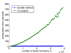
Figure 1: Computation time in seconds V.S. the number of basis functions $m$, obtained by the bundle method (blue curve) and by the interior point algorithm (green curve) for solving (9)

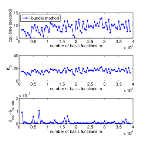
Figure 2: Computation time in seconds of the bundle method V.S. the number of basis functions $m$ (top), number of iterations $K_{0}$ of the bundle method V.S. the number of basis functions $m$ (middle), optimal value obtained by cvx $\delta_{cvx}$ minus optimal value obtained by the bundle method $\delta_{bundle}$ V.S. the number of basis functions $m$ (bottom)

References

- [AGL08] M. Akian, S. Gaubert, and A. Lakhoua. The max-plus finite element method for solving deterministic optimal control problems: basic properties and convergence analysis. SIAM J. Control Optim., 47(2):817–848, 2008.
- [BTEGN09] Aharon Ben-Tal, Laurent El Ghaoui, and Arkadi Nemirovski. Robust optimization. Princeton Series in Applied Mathematics. Princeton University Press, Princeton, NJ, 2009.
- [BV04] Stephen Boyd and Lieven Vandenberghe. Convex optimization. Cambridge University Press, Cambridge, 2004.
- [CL84] M. G. Crandall and P.-L. Lions. Two approximations of solutions of Hamilton-Jacobi equations. Math. Comp., 43(167):1–19, 1984.
- [DM11] P.M. Dower and W.M. McEneaney. A max-plus based fundamental solution for a class of infinite dimensional Riccati equations. In Decision and Control and European Control Conference (CDC-ECC), 2011 50th IEEE Conference on, pages 615 –620, dec. 2011.
- [Fal87] M. Falcone. A numerical approach to the infinite horizon problem of deterministic control theory. Appl. Math. Optim., 15(1):1–13, 1987. Corrigenda in Appl. Math. Optim., 23:213–214, 1991.
- [FF94] M. Falcone and R. Ferretti. Discrete time high-order schemes for viscosity solutions of Hamilton-Jacobi-Bellman equations. Numer. Math., 67(3):315–344, 1994.
- [FM00] W. H. Fleming and W. M. McEneaney. A max-plus-based algorithm for a Hamilton-Jacobi-Bellman equation of nonlinear filtering. SIAM J. Control Optim., 38(3):683–710, 2000.
- [GBY06] Michael Grant, Stephen Boyd, and Yinyu Ye. Disciplined convex programming. In Global optimization, volume 84 of Nonconvex Optim. Appl., pages 155–210. Springer, New York, 2006.
- [GMQ11] Stephane Gaubert, William M. McEneaney, and Zheng Qu. Curse of dimensionality reduction in max-plus based approximation methods: Theoretical estimates and improved pruning algorithms. In CDC-ECE, pages 1054–1061. IEEE, 2011.
- [HR00] C. Helmberg and F. Rendl. A spectral bundle method for semidefinite programming. SIAM J. Optim., 10(3):673–696 (electronic), 2000.
- [KCTT09] M.J. Todd K-C Toh and R.H. Tutuncu. Sdpt3:. a MATLAB software for semidefinite-quadratic-linear programming, page http://www.math.nus.edu.sg/ mattohkc/sdpt3.html, 2009.
- [Kiw90] Krzysztof C. Kiwiel. Proximity control in bundle methods for convex nondifferentiable minimization. Math. Programming, 46(1, (Ser. A)):105–122, 1990.
- [KKB07] Kwangmoo Koh, Seung-Jean Kim, and Stephen Boyd. An interior-point method for large-scale -regularized logistic regression. J. Mach. Learn. Res., 8:1519–1555, 2007.
- [LNN95] Claude Lemaréchal, Arkadii Nemirovskii, and Yurii Nesterov. New variants of bundle methods. Math. Programming, 69(1, Ser. B):111–147, 1995. Nondifferentiable and large-scale optimization (Geneva, 1992).
- [Lof04] J. Lofberg. Yalmip : a toolbox for modeling and optimization in matlab. In Computer Aided Control Systems Design, 2004 IEEE International Symposium on, pages 284–289, 2004.
- [LV07] Zhang Liu and L. Vandenberghe. Low-rank structure in semidefinite programs derived from the kyp lemma. In Decision and Control, 2007 46th IEEE Conference on, pages 5652–5659, 2007.
- [McE06] W. M. McEneaney. Max-plus methods for nonlinear control and estimation. Systems & Control: Foundations & Applications. Birkhäuser Boston Inc., Boston, MA, 2006.
- [McE07] W. M. McEneaney. A curse-of-dimensionality-free numerical method for solution of certain HJB PDEs. SIAM J. Control Optim., 46(4):1239–1276, 2007.
- [MDG08] W. M. McEneaney, A. Deshpande, and S. Gaubert. Curse-of-complexity attenuation in the curse-of-dimensionality-free method for HJB PDEs. In Proc. of the 2008 American Control Conference, pages 4684–4690, Seattle, Washington, USA, June 2008.
- [MS07] M.Grant and S.Boyd. Cvx:. Matlab software for dis- ciplined convex programming (web page and software)., page http://standford.edu/ boyd/cvx, 2007.
- [RW98] R. Tyrrell Rockafellar and Roger J.-B. Wets. Variational analysis, volume 317 of Grundlehren der Mathematischen Wissenschaften [Fundamental Principles of Mathematical Sciences]. Springer-Verlag, Berlin, 1998.
- [SGJM10] Srinivas Sridharan, Mile Gu, Matthew R. James, and William M. McEneaney. Reduced-complexity numerical method for optimal gate synthesis. Phys. Rev. A, 82:042319, Oct 2010.
- [SNW12] S. Sra, S. Nowozin, and S.J. Wright. Optimization for Machine Learning. Neural information processing series. MIT Press, 2012.
- [SZ92] Helga Schramm and Jochem Zowe. A version of the bundle idea for minimizing a nonsmooth function: conceptual idea, convergence analysis, numerical results. SIAM J. Optim., 2(1):121–152, 1992.
- [WHJ09] Ragnar Wallin, Anders Hansson, and Janne Harju Johansson. A structure exploiting preprocessor for semidefinite programs derived from the Kalman-Yakubovich-Popov lemma. IEEE Trans. Automat. Control, 54(4):697–704, 2009.