Sussing Merger Trees: the influence of the halo finder

Abstract

Merger tree codes are routinely used to follow the growth and merger of dark matter haloes in simulations of cosmic structure formation. Whereas in Srisawat et. al. we compared the trees built using a wide variety of such codes here we study the influence of the underlying halo catalogue upon the resulting trees. We observe that the specifics of halo finding itself greatly influences the constructed merger trees. We find that the choices made to define the halo mass are of prime importance. For instance, amongst many potential options different finders select self-bound objects or spherical regions of defined overdensity, decide whether or not to include substructures within the mass returned and vary in their initial particle selection. The impact of these decisions is seen in tree length (the period of time a particularly halo can be traced back through the simulation), branching ratio (essentially the merger rate of subhaloes) and mass evolution. We therefore conclude that the choice of the underlying halo finder is more relevant to the process of building merger trees than the tree builder itself. We also report on some built-in features of specific merger tree codes that (sometimes) help to improve the quality of the merger trees produced.

1 Introduction

The backbone of any semi-analytical model of galaxy formation is a merger tree of dark matter haloes. Some modern semi-analytical codes (Croton et al., 2006; Somerville et al., 2008; Monaco et al., 2007; Henriques et al., 2009; Benson et al., 2012) rely on purely analytical forms such as Press & Schechter (1974) or Extended Press-Schechter (Bond et al., 1991) –see Jiang & van den Bosch (2013) for a recent comparison of such methods–, while other codes take as input halo merger trees derived from large numerical simulations (see Roukema et al. (1997); Lacey & Cole (1993) for the historical origin of both approaches). Therefore, stable semi-analytic models require well-constructed and physically realistic merger trees: haloes should not dramatically change in mass or size, or jump in physical location from one step to the next. There are two main steps required for the production of merger trees from a $N$-Body simulation; firstly each output timeslice from a simulation needs to be analysed to produce a halo catalogue, a step performed by a halo finding algorithm. Secondly these halo catalogues need to be linked together across snapshots by a tree building algorithm to construct a merger tree. It is this final merger tree that is taken as input by a semi-analytical model.

The properties of the merger trees built using a variety of different methods has been addressed in the first ever comparison of tree builders by Srisawat et al. (2013), a paper that emerged from our Sussing Merger Trees workshop. While we observed that different tree building algorithms produce distinct results, the influence of the underlying halo catalogue (the first stage of the the two step process mentioned above) still remained unanswered. This is nevertheless an important question as different groups rely on their individual pipelines, which often includes their own simulation software, halo finding method and tree construction algorithm before the trees are fed to a semi-analytical model to obtain galaxy catalogues.

In a series of comparisons of (sub-)halo finders (e.g. Knebe et al., 2011, 2013a; Onions et al., 2012; Onions et al., 2013; Elahi et al., 2013), which are all summarised in Knebe et al. (2013b), we have seen that there can be substantial variations in the halo properties depending on the applied finder. This will certainly leave an imprint when using the catalogue to construct merger trees. As a fixed input halo catalogue was used for our first tree builder comparison the question remains; to what extent are merger trees sensitive to the supplied halo catalogue?

In this work we include both steps of the tree building process, i.e. we will apply a set of different tree builders to a range of halo catalogues constructed using a variety of object finders. Please note that the underlying cosmological simulation remains identical in all instances studied here. We are investigating how much of the scatter in the resulting merger trees that form the input to semi-analytical models stems from the tree building code and how much stems from the halo finder. Or put differently, is a merger tree more affected by the choice of the code used to generate the tree or the code used to identify the dark matter haloes in the simulation?

In what follows, the input halo catalogues and the respective finders they originate from will be presented in Section 2. In Section 3 we will then give a brief description of the merger tree building codes. Our results will be reported in Section 4 and Section 5. We close with discussion and our conclusions in Section 6.

2 Input halo catalogues

The halo catalogues used for this paper are extracted from 62 snapshots of a cosmological dark-matter-only simulation undertaken using the Gadget-3 $N$-body code (Springel, 2005) with initial conditions drawn from the WMAP-7 cosmology (Komatsu & et al., 2011). We use $270^{3}$ particles in a box of comoving width $62.5$ $h^{-1}$ Mpc/h, with a dark-matter particle mass of $m_{p}=9.31\times 10^{8}h^{-1}$M_⊙. We use 62 snapshots (000,…,061) evenly spaced in $log\,a$ from reshift 50 to redshift 0.

While in previous comparison projects (e.g. Knebe et al., 2011, 2013b; Onions et al., 2012) we forced the same mass definition (or even used a common post-processing pipeline to assure this), we did not request any such thing this time, i.e. every halo finder was allowed to use its own mass definition.

On the one hand, AHF and Rockstar define a spherically truncated mass through

$$M_{\rm ref}(<R_{\rm ref})=\Delta_{\rm ref}\times\rho_{\rm ref}\times\frac{4\pi}{3}R_{\rm ref}^{3}\ ,$$ (1)

adopting the values $\Delta_{\rm ref}=200$ and $\rho_{\rm ref}=\rho_{\rm crit}$ (we will call this mass $M_{200c}$) and iteratively removing particles not bound to the structure. On the other hand, HBThalo and SUBFIND return arbitrarily shaped self-bound objects based upon initial Friends-of-Friends (FoF) groups, assigning them the mass of all (i.e. no spherical truncation) particles gravitationally bound to the halo.

Furthermore, some halo finders include the mass of any bound substructures in the main halo mass whereas others do not include the mass of any bound substructures. Technically, finders for which particles can only belong to one halo are termed exclusive while finders for which particles can belong to more than one halo are termed inclusive. As substructures can typically account for 10% of the halo mass this choice alone can make a substantial difference to the halo mass function.

Given these definitions we can now describe the general properties of the halo finders applied to the data:

• AHF (Gill et al., 2004; Knollmann & Knebe, 2009) is a configuration-space Spherical Overdensity (SO) adaptive mesh finder. It returns inclusive gravitationally bound haloes and subhaloes spherically truncated at $R_{200c}$ (thus, the mass returned is $M_{200c}$).

• HBThalo (Han et al., 2012) is a tracking algorithm working in the time domain that follows structures from one timestep to the next. It returns exclusive arbitrarily shaped gravitationally bound objects. It uses FoF groups for the initial particle collection.

• Rockstar (Behroozi et al., 2013b) is a phase-space halo finder. A peculiarity of this code is that –unlike AHF, HBThalo and SUBFIND– the mass returned for a halo does not correspond to the sum of the mass of the particles listed as belonging to it. While it uses the same mass definition as AHF (inclusive bound $M_{200c}$ mass), the particle membership list of the halo is exclusive and is made up of particles close in phase-space to the halo centre.

• SUBFIND (Springel et al., 2001) is a configuration-space finder using FoF groups as a starting point which are subsequently searched for subhaloes. It returns arbitrarily shaped exclusive self-bound main haloes, and arbitrarily shaped self-bound subhaloes that are truncated at the isodensity contour that is defined by the density saddle point between the subhalo and the main halo.

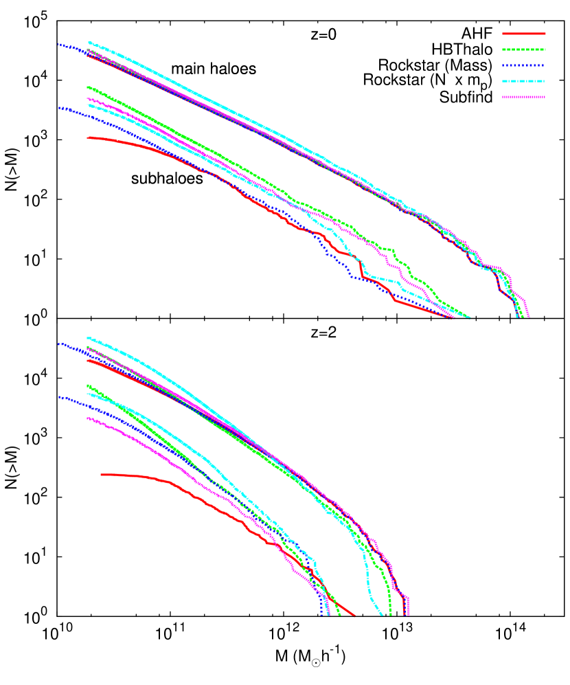
Figure 1: Cumulative mass functions at redshift $z=0$ (upper panel) and $z=2$ (lower panel) for the four halo finders. There are two lines for Rockstar corresponding to the two mass definitions discussed in the text: one corresponding to $M_{200c}$ (Mass) and one based upon the particle list ($N\times m_{p}$, being $N$ the number of particles and $m_{p}$ the particle mass). The upper set of curves in each panel is based upon main haloes whereas the lower set of curves in each panel refers only to subhaloes.

To give an impression of the differences in the halo catalogues, we present in Figure 1 the cumulative mass function for the four halo finders at redshift $z=0$ (upper panel) and $z=2$ (lower panel); we further separate subhaloes from main haloes and present their cumulative mass spectrum in the upper and lower set of curves of each panel, respectively. We have set a threshold of 20 particles (equivalent to $M=20m_{p}=1.86\times 10^{10}h^{-1}M_{\sun}$) for haloes to be considered. In order to highlight the peculiarity of Rockstar (for which the returned mass does not correspond to the sum of the mass of the particle membership) we have plotted two lines for Rockstar: one based upon summing individual particle masses (cyan dash-dotted) and one with the mass $M_{200c}$ as returned by Rockstar (blue dotted, extending to masses below the 20 particle threshold). Given that some tree builders only use particle membership information for a halo whereas others combine this with a table of global properties (including halo mass), this choice of mass definition will also contribute to the differences in the final trees.

We find that other than for the largest 100 main haloes the different mass definitions make little difference unless the mass taken from the returned Rockstar particle membership is used. This mass is systematically higher that the other estimates (and Rockstar’s own returned mass). The differences in mass for main haloes are slightly more pronounced at $z=2$.

For subhaloes there are noticeably different mass functions: AHF is incomplete at the low-mass end, with a trend that appears to worsen as the redshift increases. However, despite generally finding more subhaloes the other finders do not appear to have converged to a common set. Part of this relates to the rather ambiguous definition of subhalo mass: whereas for main haloes it simply appears to be a matter of choice for $\Delta_{\rm ref}$ and $\rho_{\rm ref}$ (or some other well-defined criterion for virialisation/boundness/linkage), subhaloes – due to the embedding within the inhomogeneous background of the host – cannot easily follow any such rule. Again, each finder has been allowed to pick its favourite definition for subhalo mass. But please note that the variations seen here are not the prime focus of this study; they should nevertheless be taken into account when interpreting the results presented and discussed below. Further, the scatter in subhalo mass functions seen in previous comparisons was much reduced due to the use of a common post-processing pipeline that ensured a unique subhalo mass definition (Onions et al., 2012; Onions et al., 2013; Knebe et al., 2013b).

All these differences should and will certainly leave an imprint and be reflected in the outcome when building merger trees.

3 Merger Tree Building Codes

The participating merger tree building codes have been extensively described and classified in the original comparison paper (Srisawat et al., 2013). But as not all merger tree builders from the original comparison engaged in this particular study and for completeness we briefly describe the participating tree building codes here.

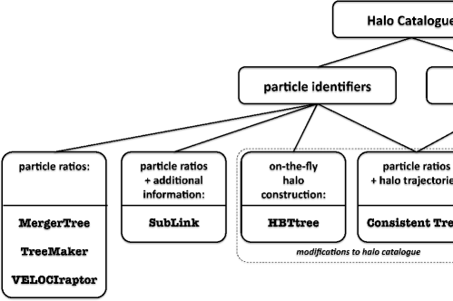
Figure 2: A summary of the main features and requirements of the different merger tree algorithms. For details see the individual descriptions in the text.

As a lot of the underlying methodology is similar across the various codes used here we have tried to capture the main features and requirements in Figure 2. We first categorise tree builders into either using halo trajectories (JMerge, and Consistent Trees) or individual particle identifiers (together with possibly some additional information; all remaining tree builders). Consistent Trees is the only method that utilises both types of approach. HBT constructs halo catalogues and merger trees at the same time as it is a tracking finder that follows structures in time. A cautionary note regarding HBT: it can be applied both as a halo finder or a tree builder and includes elements of both so we will always specify whether we refer to one or the other by appending ‘halo’ or ‘tree’, as necessary.

The codes themselves are best portrayed as follows:

• Consistent Trees forms part of the Rockstar package. It gravitationally evolves positions and velocities of haloes between timesteps, making use of information from surrounding snapshots to correct missing or extraneous haloes in individual snapshots (Behroozi et al., 2013c).

• HBTtree is built into the halo finder HBT. It identifies and tracks objects at the same time using particle membership information to follow objects between output times.

• JMerge only uses halo positions and velocities to construct connections between snapshots, i.e. haloes are moved backwards/forward in time to identify matches that comply with a pre-selected thresholds for mass and position changes.

• MergerTree forms part of the AHF package and cross-correlates particle IDs between snapshots.

• SubLink tracks particle IDs in a weighted fashion, giving priority to the innermost parts of subhaloes and allowing branches to skip one snapshot if an object disappears.

• TreeMaker consists of cross-comparing (sub)haloes from two consecutive output times by tracing their exclusive sets of particles.

• VELOCIraptor is part of the VELOCIraptor/STF package and cross-correlates particle IDs from two or more structure catalogues.

Two codes were allowed to modify the original catalogue: Consistent Trees and HBTtree. Consistent Trees adds haloes when it considers they are missing: i.e., the halo was found both at an earlier and at a later snapshot. Consistent Trees also removes haloes when it considers them to be numerical fluctuations: i.e., the halo does not have a descendant and both merger and tidal annihilation are unlikely due to the distance to other haloes. HBTtree for external halo finders (i.e. halo catalogues not generated by its own inbuilt routine) takes the main halo catalogue and reconstructs the substructure. This produces an exclusive halo catalogue in which the properties of the main haloes may also have changed.

The participants were asked to build merger trees starting from our input halo catalogues described in Section 2, in the same way as was done for the original comparison presented in Srisawat et al. (2013).

4 Geometry of trees

In this section we study the geometry and structure of merger trees and the resulting evolution of dark matter haloes. This includes the length of the tree (Section 4.1) and the tree branching ratio (Section 4.2). We further show graphically how halo finders and tree builders work differently, to illustrate the features found in the comparison.

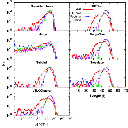
Figure 3: Histogram of the length of the main branch. The length $l$ is defined as the number of snapshots a halo can be traced back through from $z=0$. The left group of panels show the $1000$ most massive main haloes. The right group of panels show the $200$ most massive subhaloes. These number selections are equivalent to the mass cuts shown in Table 1. Different panels contain results from different tree building methods (as indicated), while within each panel there is one line for each halo finder (as marked in the legend).

4.1 Length of main branches

One of the conceptually simplest properties of a tree is the length of the main branch. It measures how far back a halo can be traced in time – starting in our case at $z=0$. This property not only relies on the performance of the halo finder and its ability to identify haloes throughout cosmic history, but also on the tree builder correctly matching the same halo between snapshots. Srisawat et al. (2013) found that the different tree building methods produced a variety of main branch lengths, ascribing some of the features to halo finder flaws. We shall verify this now.

Figure 3 shows a histogram of the main branch length $l$, defined as the number of snapshots a halo main branch extends backwards in time from snapshot $61$ ($z=0$) to snapshot $61-l$. This is roughly equivalent to an age, given that the last 50 snapshots are separated uniformly in expansion factor, $a=1/1+z$. On the left, we selected the $1000$ most massive main haloes, whereas on the right we show the results for the $200$ most massive subhaloes. The main halo population coincides from one halo catalogue to another in at least $85\%$ of the objects. The subhalo population is more complicated and, in some cases, they only agree in $15\%$ of the objects from one finder to another. However, if we focus on comparing AHF with Rockstar or HBThalo with SUBFIND, we find a better agreement between catalogues, rising to $\sim 95\%$ for main haloes and $\sim 70\%$ for subhaloes. Due to these differences, the applied number threshold translates to mass thresholds $M_{th}$ that are different from finder to finder (see also Figure 1); we therefore list the corresponding values in Table 1. Furthermore, when using HBTtree, the individual masses of the haloes can change and so does the mass threshold. In what follows we will consistently use these mass thresholds, even at higher redshift.

	AHF	HBThalo	Rockstar	SUBFIND
$M_{th}^{\rm main}$	$7.93$	$8.25$	$7.90$	$9.61$
$M_{th,\rm HBT}^{\rm main}$	$7.52$	$8.25$	$10.64$	$8.30$
$M_{th}^{\rm sub}$	$3.09$	$6.91$	$3.00$	$5.30$
$M_{th,\rm HBT}^{\rm sub}$	$2.75$	$6.91$	$2.68$	$5.90$

Table 1: Mass threshold in units of $10^{11}h^{-1}M_{\sun}$ needed to select at $z=0$ the $1000$ most massive main haloes (rows 1 and 2) and the $200$ most massive subhaloes (rows 3 and 4) for different halo finders (columns). Odd rows show the threshold for a general tree builder, whereas even rows show the threshold for HBTtree.

As expected by the hierarchical structure formation scenario induced by cold dark matter, most large mass objects can be traced back to high redshift. This is not surprising and has already been reported in our previous comparison, but here we can appreciate that this result depends on the choice of the halo finder and we will elaborate on this below.

As a general observation, for both main haloes and subhaloes, it is apparent that HBThalo leads to the best results: nearly all massive haloes are found and followed from an early origin. We attribute this to the fact that by its very nature as a tracking finder HBThalo is designed with the intention of building a merger tree in mind. SUBFIND tends to give similar results but with occasional early truncation. These truncations become more pronounced for AHF and Rockstar. Further, AHF tends to terminate each tree slightly earlier, even if it was well followed back in time, because of the incompleteness at low mass end (Figure 1). For AHF missing low-mass objects at high redshift cannot be the small progenitors of the high-mass low-redshift objects followed in Figure 3.

Differences between subhaloes and main haloes are also apparent. First, the subhalo curves in general appear more noisy, in part due to having fewer objects, but also because they are always placed in a more complicated environment which enhances the stochasticity. The difficulty in following subhaloes then causes more cases with low $l$, especially for AHF and Rockstar. One could naively think his excess of low l subhaloes for AHF and Rockstar could be the result of a much smaller $M_{th}^{sub}$ threshold (see Table 1). However, we verified that using the same threshold for all catalogues, only mitigates that difference without completely erasing it.

Subhalo finding becomes especially difficult as the subhalo approaches the centre of the host halo, as has been shown in Fig.4 of Muldrew et al. (2011) and Fig.7 of Onions et al. (2012). In particular, SUBFIND underestimates the mass of subhaloes close to the centre of their host halo. Given that the $200$ most massive subhaloes are not the same for all finders, the subhaloes selected for SUBFIND tend to be further from the host halo centres (not explicitly shown here), and therefore they are easier to trace. AHF and especially Rockstar find many (massive) subhaloes near the centre but, due to the difficulties in that region, a fraction of them cannot be provided with a credible progenitor in an earlier snapshot, resulting in early tree termination. Finally, the HBThalo selection is composed of subhaloes at short, medium and large distances from the host halo centre but, by construction, they are always required to be trackable.

On the tree builder side, JMerge allows haloes to only shrink their mass by a factor of up to 0.7 and to grow by a factor of up to 4 in one snapshot, and it estimates their trajectories from global quantities (Section 3). This artificially truncates main branches too early for massive objects when it loses track of haloes. This effect is enhanced for subhaloes, whose trajectories are difficult to estimate due to the non-linear environment and the fact that their mass is more likely to grow or shrink abruptly (Section 5). Consistent Trees and HBTtree essentially eliminate the low-$l$ cases for nearly all the haloes (and subhaloes). This is due to their freedom to modify the catalogue in such a way as to avoid exactly these occurrences.

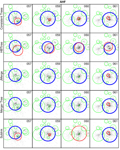
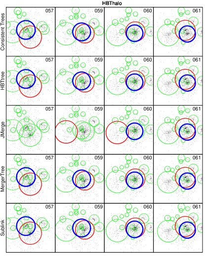
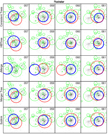
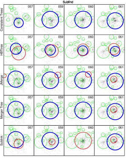
Figure 4: Projected image of a $1.2$ Mpc/h-side cube from the $N$-Body simulation. Haloes are represented by circles of radius corresponding to $R_{200c}$. This is an example of a merger between two haloes that are found at $z=0$ (snapshot 061) and linked across snapshots by the tree builders: the blue (thickest line) and red (intermediate thick line) colours represent the two trees. Other haloes found are represented in green (thinest line). Each subfigure presents a single halo finder, with each row representing the indicated tree builder. In each row time evolves from left to right, with each cell a different snapshot (labeled at the top right corner of the cell). Note that the missing tree builders all gave the same result as MergerTree.

In order to better illustrate the factors that influence the main branch length, $l$, we present in Figure 4 a graphical representation of the performance of the various halo finders and tree builders. The figure shows a projected $1.2$ Mpc/h-side cube extracted from the $N$-Body simulation with the particles (dots), the haloes found (circles), and the construction of two trees (specific thickness and colour). This slice shows two haloes of similar size passing through each other in the process of a merger (the same merger as shown in Fig.4 of Srisawat et al., 2013). These two haloes are identified at $z=0$ by a thick blue line and an intermediate thickness red line, and then traced back by the merger tree. For this example MergerTree, TreeMaker and VELOCIraptor gave identical results and so we only show the MergerTree result.

We find a wide variety of situations: in some cases every halo is correctly traced (e.g. Consistent Trees with AHF) but in others the tracing fails (e.g. JMerge with AHF). In the success or failure of the tracing the influence of both the halo finder and the tree builder are important. The effect of the tree builder was already reported in Srisawat et al. (2013), so here we focus on emphasising the dependence on the halo finder:

• AHF considers one of the merging haloes to be the main halo (blue) and the other to be a subhalo (red). In snapshot 060 the subhalo found is quite small, so that most of the tree building codes do not link it with the (much larger) halo in the next snapshot (061). In simple codes (JMerge, MergerTree… ) this leads to an artificial truncation of the tree. Consistent Trees artificially adds one halo to snapshot 060 to replace the small subhalo whereas SubLink jumps snapshot 060 for this object. In this way both codes continue the tree. HBTtree recomputes the substructure, creating a more trackable subhalo.

• HBThalo is able to identify at snapshot 060 two big and well defined haloes of almost the same size (only possible for exclusive halo catalogues). This is due to the tracking nature of the finder and ensures the correct follow-up by most tree builders. Only JMerge encounters problems due to the non-smooth trajectories of the haloes.

• Rockstar uses phase-space information so that even when the haloes are overlapping (snapshot 060) it is able to distinguish them by their velocities. This allows almost all tree codes (besides JMerge) to follow the evolution of the haloes.

• SUBFIND gives similar problems to AHF: the subhalo at snapshot 060 is too small to be considered a credible progenitor. For this catalogue, Consistent Trees is not able to deal with it and completely removes the red tree. HBTtree patches over that problem the usual way while JMerge associates the halo to a progenitor incorrectly and MergerTree truncates the tree. SubLink, by omitting snapshot 060, is able to follow the history correcty.

This example neatly illustrates the difficulties that arise when dealing with subhaloes. However, the left panel of Figure 3 tells us that there are also situations in which the main halo branch is truncated. We studied several of these cases and found two main types: in the first type the main halo lies in the vicinity of a bigger halo, and is likely to enter it and become a subhalo within the next few snapshots. In this case the problems encountered are similar to those illustrated in the subhalo example above, but here the infalling halo is still classified as a main halo at $z=0$. The other type occurs when at some point the halo was wrongly associated to some other smaller halo as happened with the red halo in Figure 3 for the combination JMerge-HBThalo. In this case the incorrect halo assignment never gets corrected and typically the much smaller halo has a much shorter prior history.

Already at this stage of the analysis we can draw some conclusions from this subsection:

• In general, the influence of the halo finder is at least as (if not more) important than the tree building algorithm.

• Main haloes are easier to trace.

• The way the halo finder deals with substructure is crucial for merger trees.

• Tree building tricks such as the creation of artificial haloes or omitting snapshots help in some cases, but are not infallible.

• AHF and Rockstar catalogues lead to earlier tree truncation for most tree builders. This is especially true for subhaloes, because they try to find subhaloes close to the host halo centre and are not able to provide them with credible progenitors.

• SUBFIND tends to find more subhaloes in the outer regions of the host, which are easier to track.

• HBT appears to be very well designed to not truncate a tree too early, both as a halo finder and as a tree builder (as seen in Figure 3 and 4).

• Consistent Trees also stands out in avoiding low-$l$ cases (Figure 3).

• JMerge faces problems in complex environments.

4.2 Branching ratio

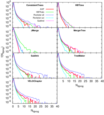
Figure 5: Normalised histograms of the number of direct progenitors $N_{\rm dprog}$ for all haloes from $z=0$ to $z=2$ (snapshots from $061$ to $031$). Each panel corresponds to a single tree building method, within each panel each line represents a halo catalogue as indicated. For Rockstar we show two lines, one with all the haloes (’Rockstar all’) and one where haloes with mass lower than $20\ m_{p}$ were removed (’Rockstar cut’).

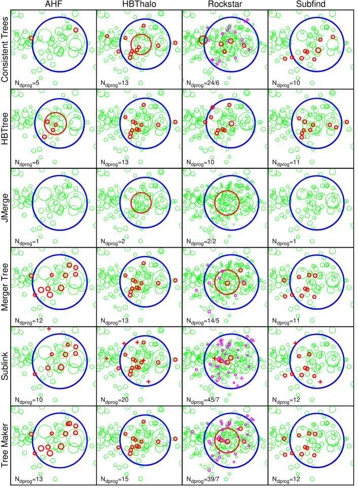
Figure 6: Projected image of a $3$ Mpc/h-side cube from snapshot 049 centred on one of the most massive objects ($M>10^{14}h^{-1}M_{\sun}$) for all the combinations of halo finder (column) and tree builder (row). VELOCIraptor gives the same results as TreeMaker, so it was omitted. All blue (thickest line), red (intermediate-thick line), and magenta (intermediate-thin line) circles (of size $R_{200c}$) together with crosses represent haloes that will merge into the same halo in snapshot 050. The blue halo is the main (and the biggest) progenitor, red and magenta circles are the remainder of direct progenitors (at snapshot 049), crosses (only for SubLink) represent haloes found in snapshot 048 but not in snapshot 049 which also merge into the same halo at 050. Haloes in magenta have mass below $20m_{p}$ (only possible for Rockstar), whereas red haloes have larger masses. Green (thinest line) circles are other haloes in the volume displayed. The label at the left-bottom corner of each cell indicates the number of progenitors found for that combination, some of which may be missing if they are not in the visible volume. For Rockstar we show two numbers, the first one lists all haloes, the second when only those with mass larger than $20m_{p}$ are considered.

Another simple tree property, which is nevertheless very important for characterising the structure or geometry of a tree, is the number of direct progenitors $N_{\rm dprog}$ (or local branches) that a halo typically has. Figure 5 shows the normalised (divided by the total number of events) histogram of $N_{\rm dprog}$ for all haloes in the range $0\leq z\leq 2$. For all the various combinations of tree building method and halo finder the most common situation is to have just one single progenitor, corresponding to a halo having no mergers on this step (which can happen multiple times during a haloes lifetime). The second most common situation is for a halo to have no progenitors, which corresponds to a halo passing above the detection threshold and appearing for the first time, which can happen only once. As for other properties studied in this paper, our results would certainly change if we were to use a different set of output times, so the importance does not lie in the individual tree results, but in their differences. For an elaborate study of the optimal choice for the temporal spacing of snapshots to construct merger trees we refer the reader to our upcoming paper (Wang Y. et al., in prep.) or to past studies on the topic (Benson et al., 2012).

It is noticeable that the Rockstar catalogue (blue dotted line) yields a tree with significantly large branching ratio for the tree builders SubLink, TreeMaker, and VELOCIraptor. Also, besides using a very similar technique, MergerTree shows a more moderate branching ratio. By removing objects with mass lower than $20m_{p}$ (cyan dash-dotted line), we verified that this high branching ratio is related to objects with very low mass as these high-$N_{\rm dprog}$ cases disappear. Recall that, even though all the halo finders cut their catalogue at 20 particles, for Rockstar the mass $M_{200c}$ can be lower if some of those particles lay outside $R_{200c}$. This small change, in general, moves the curves for Rockstar from the highest branching ratio to the lowest one. Note that the mass limited tree shown in cyan is not equivalent to the other trees because the catalogue was reduced after running the tree building algorithm on it, hence giving non-self-consistent trees. Nevertheless, we do not expect great variations in Figure 5 between the cyan line and a fully self-consistent tree with the same mass limit. This serves as an illustration of the great influence of the lower mass limit, pointing out again the importance of the input halo catalogue in the resulting tree construction.

To illustrate a high branching ratio case we have selected one of the extreme cases with $N_{\rm dprog}>30$ in Figure 6. It corresponds to one of the two most massive haloes (depending on the halo finder) at snapshot 050 (z=0.32). Figure 6 shows all the direct progenitors of that halo and other haloes found in the area. The blue (thickest) halo is the main and most massive progenitor in the plot. The red (intermediate-thick) and magenta (intermediate-thin) circles represent other direct progenitors at snapshot 049 while green (thinest) circles represent other (sub)haloes detected in the same region. Magenta is used for haloes whose mass is below $20m_{p}$ (only possible for Rockstar), while red haloes have larger mass. SubLink also has haloes that were found at snapshot 048, but were not linked in snapshot 049, which were linked to the big halo at snapshot 050; these are marked as crosses.

Figure 6 tells us that, when comparing different halo catalogues, $N_{\rm dprog}$ tends to be correlated to the number of (small) haloes available to be absorbed, i.e. the more green haloes we find the more merging (red and magenta) haloes we find. We further confirm that most secondary progenitors (red and magenta circles) are subhaloes of the main progenitor (blue circle) and lie within $R_{200c}$. However, in some cases secondary progenitors were found outside the volume displayed (e.g. the halo missing in Consistent Trees with AHF). But in general, the properties of these haloes fit into the standard merging picture in which haloes approaching a bigger one become satellites (subhaloes), lose mass via tidal stripping and are eventually totally absorbed.

If all the available haloes are considered, Rockstar is the catalogue with most small haloes, leading to a higher branching ratio, which drops when removing the low mass haloes. HBThalo is also able to discern more substructure, yielding a slightly higher $N_{\rm dprog}$ than SUBFIND and AHF.

From the tree building point of view we remark that SubLink, with the possibility of omitting one snapshot, increases $N_{\rm dprog}$ considerably for the two catalogues with more substructure: Rockstar and HBThalo. HBTtree, in modifying the catalogue, tends to recover the halo set generated by HBThalo. This effect is more noticeable in the case of SUBFIND because it is also based on FoF catalogues (Section 2). JMerge shows very little branching ($N_{\rm dprog}=1$ or $2$) because by construction it never associates a small merging halo with a much bigger one. It rather associates the infalling halo with another small halo.

Note, however, that this was a very extreme case and that Figure 6 is not necessarily representative of the statistics seen in Figure 5, rather it helps to understand the kind of factors that influence the branching ratio.

5 Mass Evolution

The mass evolution of haloes is an important input for semi-analytical models of galaxy formation. In this section we will study it through mass growth (Section 5.1) and fluctuations in mass (Section 5.2).

5.1 Mass Growth

Mass growth can be characterised by the discretised logarithmic growth, defined as:

$$\frac{\rm{d}\log\ M}{\rm{d}\log\ t}\approx\alpha_{M}(k,k+1)=\frac{(t_{k}+t_{k+1})(M_{k+1}-M_{k})}{(t_{k+1}-t_{k})(M_{k+1}+M_{k})}$$ (2)

where $k$ and $k+1$ are a halo and its descendant, with masses $M_{k}$ and $M_{k+1}$ at times $t_{k}$ and $t_{k+1}$, respectively (Srisawat et al., 2013). In order to reduce the range of possible values of this variable to the finite interval $(-1,+1)$, we define:

$$\beta_{M}=\frac{1}{\pi/2}\rm{arctan}(\alpha_{M})$$ (3)

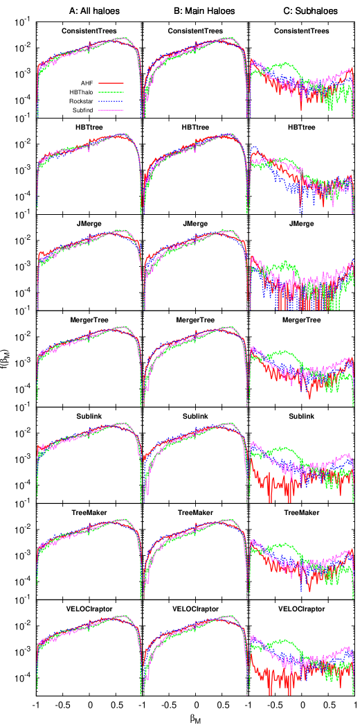
Figure 7: Mass growth distribution between two snapshots, $\beta_{M}$, related to the logarithmic mass growth through Equation 3, for haloes that can be identified at $z=0$, with mass $M>M_{th}$ at both output times. We distinguish 3 populations: $A$ which contains all haloes with $M_{th}=M^{main}_{th}$, $B$ with only main haloes and $M_{th}=M^{main}_{th}$, and $C$ with only subhaloes and $M_{th}=M^{sub}_{th}$. $M_{th}$ is tabulated in Table 1 for the different halo finders. Each row displays a different tree building algorithm (as indicated). Each halo finder has its own line style as indicated in the legend. The distribution is computed as a histogram, normalised by the total number of events found by the corresponding halo finder for the population $A$.

Figure 7 shows the distribution of $\beta_{M}$ for three populations: all haloes ($A$, on the left), main haloes ($B$, in the centre) and subhaloes ($C$, on the right). All distributions have been normalised by the total number of events found in halo sample $A$ in each case. Selection is done as follows: all the haloes identified at $z=0$ are traced back along the main branch and at any snapshot if both a halo and its descendant are main [sub] haloes and have mass $M>M_{th}^{\rm main}$ [$M>M_{th}^{\rm sub}$] (Table 1) sum to the population $B$ [$C$]. The population $A$ is compiled similarly, but taking all pairs of haloes satisfying $M>M_{th}^{\rm main}$, regardless of being main or subhaloes. Note that the distribution $A$ is dominated by main haloes, since they are more numerous.

Within the hierarchical structure formation scenario one expects haloes to grow over time. This can be appreciated in column $A$, where the distribution of $\beta_{M}$ is skewed towards values $\beta_{M}>0$. However, there is a non-negligible number of cases ($\sim 15-30\%$) where it decreases ($\beta_{M}<0$). While mass loss could be associated with tidal stripping of subhaloes, column $B$ shows that this is not the sole explanation within this simulation: while subhaloes have an important contribution at the very far end of the distribution (corresponding to large mass losses), there are also many instances leading to $\beta_{M}<0$ for main haloes. Nevertheless, there are physical ways for main haloes to lose mass: when two main haloes approach each other, the effective radius for tidal stripping extends beyond the virial radius of the larger halo (see Behroozi et al., 2013a, for an elaborate discussion of exactly this phenomenon), thus, the small one can experience mass loss before becoming a satellite. Also, when haloes change their shape, the specific halo mass definition (e.g. $M_{200c}$ for AHF/Rockstar) of a halo finder can lead to an apparent mass loss.

The plot clearly shows that the differences across halo finders are greater than the variations introduced by the tree building method, with the exception of HBTtree (that modifies the input halo catalogue). There are two distinct classes of distribution for main haloes ($B$): on the one hand, Rockstar and AHF, and on the other hand, SUBFIND and HBThalo which have a more skewed distribution. Recall from (Section 2) that the former use an inclusive mass definition, thus, for a subhalo that just crossed the centre and is moving away, the total (inclusive) mass of the host halo can decrease if part of that subhalo crosses $R_{200c}$.

We finally remark that while subhaloes are present in our somewhat low-resolution simulation (when compared to the state-of-the-art), they contribute significantly to neither the shape nor the amplitude of the mass growth distribution shown in column $A$ (all haloes). However, their own distribution (column $C$) is interesting in its own regard: we primarily observe mass loss due to tidal stripping, i.e. an imbalance of the distribution towards negative $\beta_{M}$ values. In this case we find that whereas HBThalo follows one distribution, the other three follow their own. This reflects the inconsistency in subhalo mass functions already seen in Figure 1.

In conclusion, most of the differences in the mass growth $\beta_{M}$ can be accounted for by the choices made by the respective halo finder when defining quantities. In particular, HBThalo and SUBFIND agree best with the a priori expectation from hierarchical structure formation.

5.2 Mass Fluctuations

After studying mass growth above, we quantify mass fluctuations by using

$$\xi_{M}=\frac{\beta_{M}(k,k+1)-\beta_{M}(k-1,k)}{2}$$ (4)

where ${k-1,k,k+1}$ represent consecutive timesteps. When far from zero, it implies a growth followed by a dip in mass ($\xi_{M}<0$) or vice versa ($\xi_{M}>0$). Within the hierarchical structure formation scenario this behaviour can be considered unphysical and equates to a snapshot where the halo finder might not have assigned the correct mass – though there are certainly situations where the definition of correct mass remains arguable. Nevertheless, it provides another means of quantifying the influence of the halo finder upon a merger tree.

The (normalised) distribution of $\xi_{M}$ is presented in Figure 8 in the same way as Figure 7, i.e. three distinct columns for all haloes ($A$, left), main haloes ($B$, middle), and subhaloes ($C$, right). It reconfirms most of the claims of Section 5.1. We again find the distribution is essentially independent of the tree builder (besides HBTtree) for all three populations. We find two types of distributions for main haloes ($B$): on the one hand, the SUBFIND and HBThalo catalogues give the broadest distributions and on the other hand, Rockstar and AHF have a more peaked distribution. This implies that the first pair of halo finders present more mass fluctuations ($\xi_{M}\neq 0$) than the second one. Note that this pairing is identical to the one reported in Section 5.1. And we also find (again) that subhaloes ($C$) do not provide an explanation for the wings of the mass fluctuation distribution in column $A$, even though their own plot indicates that they predominantly undergo abrupt changes, i.e. they have easily distinguished wings.

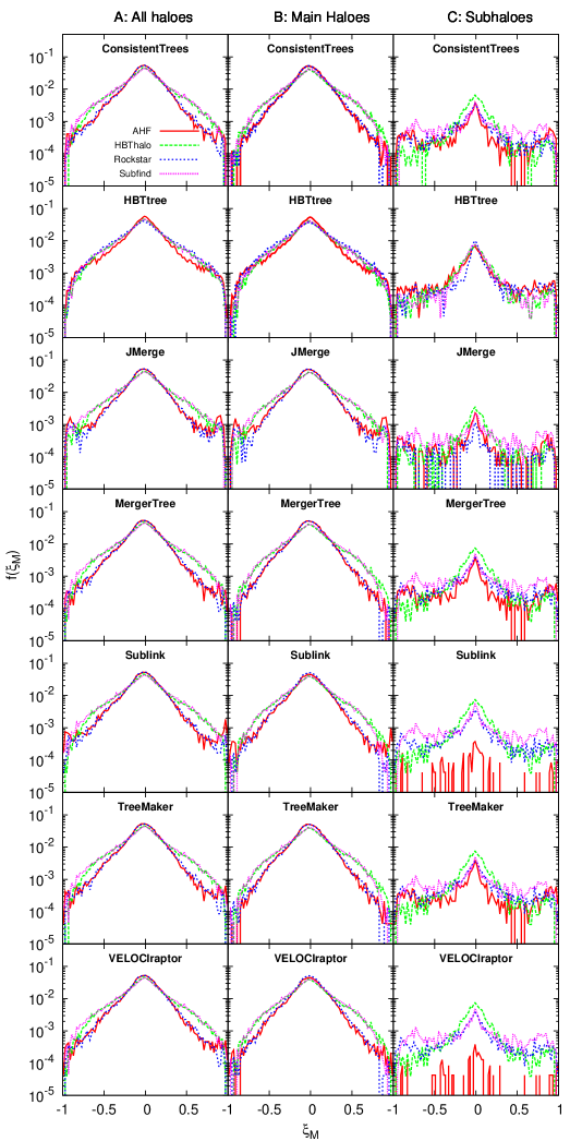
Figure 8: Distribution of mass fluctuations $\xi_{M}$ (Equation 4), for haloes found in three consecutive snapshots along a main branch that can be identified at $z=0$, with mass $M>M_{th}$ for each appearance of the halo. We distinguish 3 populations: $A$ which contains all haloes with $M_{th}=M^{main}_{th}$, $B$ with only main haloes and $M_{th}=M^{main}_{th}$, and $C$ with only subhaloes and $M_{th}=M^{sub}_{th}$. $M_{th}$ is tabulated in Table 1. Comparison is made between different tree builders (each row as labeled) and halo finders (line styles as in the legend). The distribution is computed as a histogram normalised by the total number of events for the corresponding halo finder for the population $A$.

Given that subhaloes often undergo fluctuations (column $C$ of Figure 8), this could cause fluctuations in main haloes when the mass is defined exclusively (HBThalo and SUBFIND). In order to study this effect, we selected a halo whose mass evolution is characterised by a large $\xi_{M}$ value (for the SUBFIND/HBThalo pair) in Figure 9. We localised the same object (the big blue halo) and surrounding ones (a red halo next to it and a green halo for HBT in the center) in all four halo catalogues, showing the three consecutive snapshots used for the calculation of $\xi_{M}$ given at the very right hand side of each panel. The halo undergoes a mass fluctuation for the finders HBThalo and SUBFIND, while it keeps growing for AHF and Rockstar. Figure 9 shows that, although it is true that for HBThalo/ SUBFIND the total mass of the subhaloes increases when the main halo decreases and vice versa, the fluctuation of subhalo mass is one order of magnitude smaller than the main halo fluctuation and this cannot be the sole explanation. The fact that the red halo changes from being a subhalo to a main halo and then back to a subhalo again may be related (in a non-trivial way, since masses are defined exclusively) to the mass fluctuation. For this simple (compared to Figure 4 & Figure 6) configuration of haloes, all the tree building algorithms agree in the resulting trees. We also note that even small fluctuations (10% in mass) are detected by this parameter $\xi_{M}$, in part due to an enhancement of $\xi_{M}$ at late times (cf. Equation 3 & Equation 4).

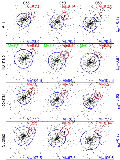
Figure 9: Projected $1$ Mpc/h-side cube containing two haloes (three for HBThalo) evolving from snapshot 058 (left column) to 059 (central column) to 060 (right column). Each row shows a different halo finder. The radius of the circle is represented proportional to the mass of the object, with an extra factor of $\times 5$ for the small (red and green) haloes. Dashed lines denote subhaloes whereas solid lines are used for main haloes. The mass of each halo is also shown in units of $10^{10}h^{-1}M_{\sun}$. At the right of each row we can see the value of $\xi_{M}$ for the big halo, which quantifies the mass fluctuation as defined by Equation 4.

5.3 Combining growth and fluctuations

To better draw any conclusion from our study of the mass evolution of main haloes we summarise results from their $\beta_{M}$ and $\xi_{M}$ statistics (Section 5.1 & Section 5.2) in Figure 10: the $x$-axis shows the fraction $f_{\beta_{M}>0}$ of objects for which $\beta_{M}>0$, whereas the $y$-axis shows the standard deviation $\sigma_{\xi_{M}}$ of $\xi_{M}$. Different sizes (or colours) now represent different tree building methods whereas the symbols stand for the input halo catalogue. The desirable feature of a tree describing hierarchical structure formation would be to have small mass loss for main haloes (high $f_{\beta_{M}>0}$) and small mass fluctuations (low $\sigma_{\xi_{M}}$), at least a priori, because we also explained physical causes for these phenomena. Note also that the quantities plotted here do not provide a substitute for the whole curve shown in Figure 7 & Figure 8, but rather capture well the features of interest as they are observed. This summary plot illustrates very well how mass evolution sensitively depends on the choice of the halo finder:

• Points for the same halo finder (symbol) group together. The small scatter amongst those groups represents the small influence of the tree building method on these magnitudes.

• HBTtree points deviate from the group, approaching the area of the HBThalo finder (crosses).

• The pair of halo finders HBThalo/SUBFIND achieves a lower rate of mass loss at the price of having more mass fluctuation than the other pair of finders AHF/Rockstar for main haloes. We relate this pairing to the mass definition of the halo finder: the former is exclusive and uses self-bound objects, whereas the latter uses inclusive spherical $M_{200c}$ objects.

We have verified that mass growth and fluctuations are intrinsically related to the mass definition. A simple change from an inclusive to an exclusive halo catalogue or from $M_{200c}$ to arbitrarily shaped haloes would change the shape of the curves seen in Figure 7 & Figure 8 and the position of the points in Figure 10. But other fundamental properties of the halo finder also leave their imprint, the evident differences between HBThalo and SUBFIND in Figure 10 are a proof of this.

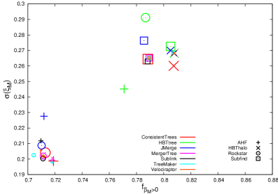
Figure 10: Summary of Figure 7 and Figure 8. On the abscissa we show the fraction of haloes for which mass grows; on the ordinate we show the standard deviation of the mass fluctuations. Only main haloes satisfying $M>M_{th}^{main}$ (Table 1) are taken into account. Every point represents a combination of a tree builder (size and colour-coded) and a halo catalogue (symbol-coded, see legend). The size of the points represents the different tree builders in decreasing order as they are listed in the legend (Consistent Trees the largest, VELOCIraptor the smallest).

6 Discussion & Conclusions

Following the first paper (i.e. Srisawat et al., 2013) in a series of articles comparing various tree building codes, we investigated the influence of the input halo catalogue on the quality of the resulting merger trees. ’Quality’ in this regard has been identified as length of the main branch, number of direct progenitors, and, quantities that are highly relevant for semi-analytical modeling, the mass growth and mass fluctuation of haloes. We also showed some specific examples of cases that aided our understanding of the influence of the halo finder and tree builder on the resulting properties of the trees.

In total, seven different tree building methods have been applied to the halo catalogues produced by four different halo finding algorithms which examined the same cosmological simulation. This produced 28 merger trees to be analysed. The influence of both groups of codes is summarised below, and the particular achievements and difficulties of the different methods discussed.

The influence of the halo finder

The primary conclusion of all the studies presented here is that the influence of the input halo catalogue is greater than the influence of the tree building method employed. This is especially clear for the mass evolution studies (Section 5) although it is also noticeable from the results of the main branch length (Section 4.1) and the studies on the branching ratio also suggest it (Section 4.2). Part of these differences are due to the fact that for this comparison we allowed the halo finders to choose their own definitions instead of unifying them as done in previous halo finder comparison projects. However, this way we find the real impact a user will encounter when choosing one or the other halo finder for his/her analysis.

Another pattern encountered along our studies is the pairing AHF/Rockstar vs. HBThalo/SUBFIND. This is very clear in the mass evolution of main haloes (central columns of Figure 7 and Figure 8, summarised in Figure 10) and can also be seen in the main branch length distribution (Figure 3). We interpret this pairing to be caused by the fundamental construction of the halo catalogues, namely spherically truncated $M_{200c}$ inclusive masses (Equation 1) for the former pair vs. self-bound exclusive objects starting from FoF groups for the latter. These differences can already be acknowledged in the main halo mass function shown in Figure 1.

The studies on the length of the tree (Section 4.1) are the cleanest test, since they do not rely on arbitrary choices such as the lower mass cut (which makes a significant difference for the branching ratio) or the mass definition (which is of great influence in the mass evolution). The tracking nature of HBThalo showed excellent results in this section, with no early truncation of (sub)haloes. Rockstar and AHF showed early truncation of trees, especially for subhaloes near the centre of their host, whereas SUBFIND did not show too much early truncation of subhaloes, because they are systematically missing in the centre of the hosts. AHF, with its poor completeness at the low-mass end led to the shortest main branches: because haloes disappear due to this incompleteness the main branches tend to end early.

The relevance of the lower mass cut was also seen in the study of the branching ratio (Figure 5 in Section 4.2). In particular, for Rockstar a cut in mass was not equivalent to a cut in the number of particles. Because of this, doing the same cut in particles as for other catalogues, the branching ratio of Rockstar was too high.

The mass evolution of haloes was found to be mostly dependent upon the mass definition employed by the halo finder. However, it is not clear which finders perform best: HBThalo/SUBFIND show less mass loss whereas AHF/Rockstar show fewer mass fluctuations. Mass evolution is intrinsically related to the way the mass is defined, and the choice of a different mass definition within the same halo finder would lead to different results.

Along these lines, note that some properties of the halo finders are simple choices that are relatively easy to change, as for example the exclusive/inclusive mass assignment or the choice of spherical haloes vs. self-bound objects. However, we have seen in Knebe et al. (2013b) that other, more fundamental, details of each halo finder (such as the initial particle collection) leave their own unique signature in the catalogue. These are practically unavoidable and hence the user has to decide upfront which halo finder best suits their needs.

The influence of the tree building method

Although we found a greater dependence on the halo finder than on the tree building method, each of the tree codes also has its own peculiarities:

• Consistent Trees in many cases is able to correct the problems posed by the finder by adding artificial haloes.

• HBTtree, when recomputing the substructure, makes haloes more trackable, improving the results.

• JMerge has problems in dealing with the motion of (sub)haloes in highly clustered environments.

• MergerTree, TreeMaker and VELOCIraptor behave very similarly, as they are based on nearly identical algorithms.

• SubLink is sometimes able to compensate for non-detection of haloes by looking at non-consecutive timesteps.

Outlook

The main outcome of the present paper is that the fundamental properties of halo finders have a major impact on the merger trees constructed from them, and that some tree building techniques can help improve those trees by correcting for halo finder defects. We pointed out the repercussions that several properties of the halo finders and tree building codes can have on the final trees. This should help the community choosing, designing or modifying their pipelines to construct merger trees idealised for their specific purposes.

It is worth mentioning that, although here we focused on the differences among the resulting merger trees, the agreement among them is nevertheless remarkable. The general features of the trees resulted as one would have expected, and are similar from one tree to another. Many times the differences between trees are only seen when plots are done on a logarithmic scale, since those differences are at the order of a few-cases for every thousand plotted.

The remaining question is how all this affects our understanding of the Universe, at least when theoretically modeling it. This series of code comparison workshops helps us exploring the degree of certainty we have when generating virtual skies. The first workshop(s) related to the identification of objects: haloes, subhaloes and galaxies. We are currently investigating the linkage between objects: the merger trees. In an ultimate step we will analyse how the different pipelines can lead to different simulated direct observables: from the merger trees we will move to the effect of semi-analytic methods and other ways to generate galaxy mock catalogues and placing them in lightcones to generate mock surveys.

References

- Behroozi et al. (2013a) Behroozi P. S., Wechsler R. H., Lu Y., Hahn O., Busha M. T., Klypin A., Primack J. R., 2013a, submitted to ApJ, arXiv:1310.2239
- Behroozi et al. (2013b) Behroozi P. S., Wechsler R. H., Wu H.-Y., 2013b, ApJ, 762, 109
- Behroozi et al. (2013c) Behroozi P. S., Wechsler R. H., Wu H.-Y., Busha M. T., Klypin A. A., Primack J. R., 2013c, ApJc, 763, 18
- Benson et al. (2012) Benson A. J., Borgani S., De Lucia G., Boylan-Kolchin M., Monaco P., 2012, MNRAS, 419, 3590
- Bond et al. (1991) Bond J. R., Cole S., Efstathiou G., Kaiser N., 1991, ApJ, 379, 440
- Croton et al. (2006) Croton D. J., Springel V., White S. D. M., De Lucia G., Frenk C. S., Gao L., Jenkins A., Kauffmann G., Navarro J. F., Yoshida N., 2006, MNRAS, 365, 11
- Elahi et al. (2013) Elahi P. J., Han J., Lux H., Ascasibar Y., Behroozi P., Knebe A., Muldrew S. I., Onions J., Pearce F., 2013, MNRAS, 433, 1537
- Gill et al. (2004) Gill S. P., Knebe A., Gibson B. K., 2004, MNRAS, 351, 399
- Han et al. (2012) Han J., Jing Y. P., Wang H., Wang W., 2012, MNRAS, 427, 2437
- Henriques et al. (2009) Henriques B. M. B., Thomas P. A., Oliver S., Roseboom I., 2009, MNRAS, 396, 535
- Jiang & van den Bosch (2013) Jiang F., van den Bosch F. C., 2013, arXiv:1311.5225
- Knebe et al. (2011) Knebe A., Knollmann S. R., Muldrew S. I., Pearce F. R., et al. 2011, MNRAS, 415, 2293
- Knebe et al. (2013a) Knebe A., Libeskind N. I., Pearce F., Behroozi P., Casado J., Dolag K., Dominguez-Tenreiro R., Elahi P., Lux H., Muldrew S. I., Onions J., 2013a, MNRAS, 428, 2039
- Knebe et al. (2013b) Knebe A., Pearce F. R., Lux H., Ascasibar Y., et al. 2013b, submitted to MNRAS, arXiv:1304.0585
- Knollmann & Knebe (2009) Knollmann S. R., Knebe A., 2009, ApJS, 182, 608
- Komatsu & et al. (2011) Komatsu E., et al. 2011, ApJS, 192, 18
- Lacey & Cole (1993) Lacey C., Cole S., 1993, MNRAS, 262, 627
- Monaco et al. (2007) Monaco P., Fontanot F., Taffoni G., 2007, MNRAS, 375, 1189
- Muldrew et al. (2011) Muldrew S., Pearce F., Power C., 2011, MNRAS, 410, 2617
- Onions et al. (2012) Onions J., Knebe A., Pearce F., Muldrew S., Lux H., Knollmann S., Ascasibar Y., Behroozi P., Elahi P., Han J., Maciejewski M., Merchán M., Neyrinck M., Ruiz A., Sgró M., Springel V., Tweed D., 2012, MNRAS, 423, 1200
- Onions et al. (2013) Onions J., Ascasibar Y., Behroozi P., Casado J., Elahi P., Han J., Knebe A., Lux H., Merchán M. E., Muldrew S. I., Neyrinck M., Old L., Pearce F. R., Potter D., Ruiz A. N., Sgró M. A., Tweed D., Yue T., 2013, MNRAS, 429, 2739
- Press & Schechter (1974) Press W. H., Schechter P., 1974, ApJ, 187, 425
- Roukema et al. (1997) Roukema B. F., Quinn P. J., Peterson B. A, 1997, MNRAS, 292, 835
- Somerville et al. (2008) Somerville R. S., Hopkins P. F., Cox T. J., Robertson B. E., Hernquist L., 2008, MNRAS, 391, 481
- Springel (2005) Springel V., 2005, MNRAS, 364, 1105
- Springel et al. (2001) Springel V., White S. D. M., Tormen G., Kauffmann G., 2001, MNRAS, 328, 726
- Srisawat et al. (2013) Srisawat C., Knebe A., Pearce F. R., Schneider A., Thomas P. A., Behroozi P., Dolag K., Elahi P. J., Han J., Helly J., Jing Y., Jung I., Lee J., Mao Y. Y., Onions J., Rodriguez-Gomez V., Tweed D., Yi S. K., 2013, MNRAS, 436, 150