Abstract

Accepting validity of self-consistent theory of localization by Vollhardt and W${\rm{\ddot{o}}}$lfle, we derive the relations of finite-size scaling for different parameters characterizing the level statistics. The obtained results are compared with the extensive numerical material for space dimensions $d=2,\,3,\,4$. On the level of raw data, the results of numerical experiments are compatible with the self-consistent theory, while the opposite statements of the original papers are related with ambiguity of interpretation and existence of small parameters of the Ginzburg number type.

The present paper continues the series of publications [1, 2, 3] devoted to a theoretical analysis of numerical algorithms used for investigation of the Anderson transition. These studies are motivated by contradiction of numerical data (see a review article [4]) with self-consistent theory by Vollhardt and W${\rm{\ddot{o}}}$lfle [5, 6], which reproduces the main body of theoretical results and according to certain arguments [7, 8] gives the correct critical behavior. In particular, the numerical results are incompatible with existence of the upper critical dimension $d_{c2}=4$, which is a rigorous consequence of the Bogoliubov theorem [9] on renormalizability of $\varphi^{4}$ theory [1]. Since numerical modelling is carried out independently by different groups [4,10-17], the presence of trivial mistakes is surely excluded; however, all numerical algorithms are empirical and not based on a serious theoretical ground.

The object for the present investigation is the scaling for level statistics [10], which currently became one of the most popular algorithms [11]–[15]. Its comparative simplicity is related with the fact that it deals only with the spectrum of the matrix Hamiltonians and does not require a calculation of eigenfunctions or conductivity.

The distribution function $P(\omega)$ for a spacing $\omega$ between the nearest levels is conveniently treated in terms of the variable

$$s=\omega/\Delta\,,\qquad\Delta=1/\nu_{F}L^{d}\,,$$

where $\Delta=\langle\omega\rangle$ is the mean level spacing in a finite system having a form of the $d$-dimensional cube of size $L$; $\nu_{F}$ is the density of states at the energy of interest (like the Fermi level). According to [10], there are three actual distributions: Wigner–Dyson $(W)$, Poisson $(P)$ and critical $(c)$ (Fig. 1):

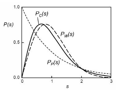
Figure 1: Distribution $P(s)$ of the nearest level spacing for Wigner-Dyson, Poisson and critical statistics. Distributions $P_{W}(s)$ and $P_{P}(s)$ intersects in points $s=0.473$ and $s=2.002$.

$$P_{W}(s)={\frac{\pi}{2}}\,s\,\exp\left(-{\frac{\pi}{4}}s^{2}\right)\,,\qquad\qquad\qquad$$

$$P_{P}(s)=\exp\left(-s\right)\,,\qquad\qquad\qquad\qquad\qquad$$

$$P_{c}(s)=\left\{\begin{array}[]{cc}\sim s\,,&s\ll 1\\ \sim\exp\left(-s/2\kappa\right)\,,&s\gg 1\end{array}\right.\,,\quad$$

which are realized correspondingly in the metallic state, the localization phase and the critical region. If the system is in the critical point, then its level distribution coincides with $P_{c}(s)$ independently of size $L$. With a small deviation from the critical point, distribution $P(s)$ changes slowly with $L$ and tends to $P_{W}(s)$ or $P_{P}(s)$ in the large $L$ limit. For a quantitative control of such evolution one can consider the integral over the large $s$ region,

$$I(s_{0})=\int_{s_{0}}^{\infty}\,P(s)ds\,,$$

and introduce the scaling parameter

$$\alpha(s_{0})=\frac{I(s_{0})-I_{W}(s_{0})}{I_{P}(s_{0})-I_{W}(s_{0})}\,,$$

which changes from zero to unity with a crossover from a metal to dielectric. If the scaling relation is postulated,

$$\alpha=F\left(L/\xi\right)\,,$$

then the critical behavior of the correlation length $\xi$ can be extracted from the evolution of $\alpha$ under the change of $L$ [10]. Analogously, one can consider the integral over the small $s$ region,

$$\tilde{I}(s_{0})=\int_{0}^{s_{0}}\,P(s)ds\,,$$

and define the scaling parameter $\tilde{\alpha}(s_{0})$ analogously to (6), which formally coincides with $\alpha(s_{0})$ due to relation $\tilde{I}(s_{0})=1-I(s_{0})$. Practically, definition (5) is traditionally used with the distinguished value $s_{0}=2.002$, corresponding to the common intersection point of three distributions (Fig.1), while definition (8) exploits a value $s_{0}=0.473$ corresponding to the second intersection point of $P_{W}(s)$ and $P_{P}(s)$.

Another variant of the scaling parameter is coefficient $A$ in the dependence

$$I(s)=\exp\left(-As\right)$$

which tends to a constant limit for large $s$; the scaling relation of type (7) can be postulated for it. The more complicated versions of scaling parameters were used in the cases $d=2$ [13] and $d=4$ [14] (see Secs. 7, 8).

The main questions are connected with scaling relations of type (7), which cannot be justified for arbitrary quantities, are certainly invalid in high dimensions and can be essentially distorted by corrections to scaling. It is shown below, that self-consistent theory of localization [5, 6] allows to establish the relations of type (7) for all introduced quantities, and the obtained scaling functions can be compared with the extensive numerical material [10]–[15]. Analogously to [1]–[3] it appears, that raw numerical data are perfectly compatible with the Vollhardt and W${\rm{\ddot{o}}}$lfle theory, while the opposite statements of the corresponding researchers are related with ambiguity of interpretation and existence of small parameters of the Ginzburg number type.

2. Quasi-Gaussian Conception

A calculation of the distribution function $P(s)$ is practically impossible for realistic models, and a theoretical analysis of the algorithm looks rather questionable. However, such analysis becomes possible, if some roughening scheme is accepted. An example of such a roughening is the quasi-Gaussian conception suggested by Altshuler et al [18].

Let $N$ be the number of levels in the interval $E$ near the energy $\epsilon_{F}$ (Fig. 2); below $\epsilon_{F}=0$ is accepted. If fluctuations of $N$ are small, one can expect a validity of the Gaussian distribution for them,

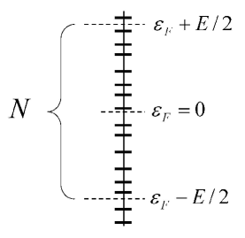
Figure 2: $N$ is the number of levels in the interval $E$.

$$P(N)\sim\exp\left\{-\frac{(N-\langle N\rangle)^{2}}{2\sigma^{2}}\right\}\,,$$

where $\sigma^{2}$ depends on $\langle N\rangle$. The probability of the event that there are no levels in the interval $E$ is given by Eq.10 with $N=0$. In terms of the introduced quantities, it means that $\omega=s\Delta$ can take any value greater than $E$; it corresponds to the integral (5) with $s_{0}=E/\Delta$. Taking into account a dependence of $\sigma^{2}$ on $\langle N\rangle=E/\Delta=s_{0}$, one has

$$I(s_{0})\sim\exp\left(-\frac{s_{0}^{2}}{2\sigma(s_{0})^{2}}\right)\,.$$

Since integration of $P(s)$ does not change the form of the exponential in (2 – 4), one can reproduce it by substitution

$$\sigma_{W}(s)^{2}=2/\pi\,,\qquad$$

$$\sigma_{P}(s)^{2}=s/2\,,\qquad$$

$$\sigma_{c}(s)^{2}=\kappa s\,.\qquad$$

On the other hand, a direct calculation of the mean square fluctuation

$$\sigma_{0}^{2}=\langle N^{2}\rangle-\langle N\rangle^{2}$$

gives

$$(\sigma_{0}^{2})_{W}=(2/\pi^{2})\ln s\,,\qquad$$

$$(\sigma_{0}^{2})_{P}=s\,,\qquad\qquad$$

$$(\sigma_{0}^{2})_{c}=\kappa_{0}s\,,\qquad\qquad$$

where the first expression is the result by Dyson [19], the second one corresponds to the Poisson distribution [20], and the third was suggested in [18] using the simple scaling arguments [21] and confirmed numerically in [11]. According to [11, 14]

$$\kappa_{0}=0.28\pm 0.03\,,\quad\kappa=0.26\pm 0.01\quad(d=3)\,,$$

$$\kappa_{0}=0.45-0.50\,,\quad\kappa\approx 0.36\qquad(d=4)\,,$$

i.e. $\kappa$ and $\kappa_{0}$ are close but not identical. A comparison of (12) and (14) shows that $\sigma^{2}$ and $\sigma_{0}^{2}$ coincide in the order of magnitude aside from the Wigner-Dyson case, where they differ by a logarithmic factor. The latter is not surprising. Abundance of the Gaussian distribution is a consequence of the central limit theorem, whose derivation shows [22], that the Gaussian form is valid near the maximum of distribution, while its tails remain not universal. The given reasoning is valid in the certain interval of the $s$ values, which are sufficiently large for realization of the exponential behavior in (2 – 4), but sufficiently small for a crude validity of the Gaussian distribution (10) in the vicinity of $N=0$. With any reasonable restrictions for $s$, one has $\ln s\sim 1$ and the order-of-magnitude coincidence of $\sigma^{2}$ and $\sigma_{0}^{2}$ is indeed valid. The two latter quantities vary in wide limits and their difference in a slow function is of a little consequence, so this function can be replaced by a constant in the accepted roughening scheme. As a result, an evolution of distribution $P(s)$ is mainly determined by the quantity $\sigma_{0}^{2}$, which allows a theoretical description (Sec. 3).

Substitution of (11) into (6) shows that for large $s_{0}$ one can neglect $I_{W}(s_{0})$, so

$$\alpha(s_{0})=\exp\left\{-\frac{s_{0}^{2}}{2\sigma_{P}^{2}}+\frac{s_{0}^{2}}{2\sigma^{2}}\right\}=$$

$$=\exp\left\{-s_{0}\frac{\sigma_{P}^{2}-\sigma^{2}}{\sigma^{2}}\right\}\,,$$

and $\alpha(s_{0})$ differs from zero only for $\sigma_{P}^{2}-\sigma^{2}\ll\sigma_{P}^{2}$ and practically disappears in the Wigner-Dyson range $\sigma^{2}\sim\sigma_{W}^{2}$. A comparison of (11) and (9) shows that

$$A=\frac{s}{2\sigma^{2}}=\frac{\sigma_{P}^{2}}{\sigma^{2}}\,,$$

so parameters $\alpha(s_{0})$ and $A$ are determined by the single combination $\sigma^{2}/\sigma_{P}^{2}$; the same is true for the more complicated scaling parameters (Secs. 7, 8).

3. Diagrammatic Approach

A calculation of $\sigma_{0}^{2}$ in the framework of the diagrammatic technique was considered by Altshuler and Shklovskii [23]. Having in mind the subsequent generalizations, we discuss in details the selection principle of diagrams.

The number of levels $N$ in the interval $E$ is expressed through the exact density of states $\nu(\epsilon)$ in a finite system

$$N=L^{d}\,\int\limits_{-E/2}^{E/2}\nu(\epsilon)d\epsilon\,,\quad\nu(\epsilon)=L^{-d}\sum\limits_{n}\,\delta(\epsilon-\epsilon_{n})\,,$$

while its mean square fluctuation

$$\sigma_{0}^{2}=L^{2d}\,\int\limits_{-E/2}^{E/2}d\epsilon_{1}\int\limits_{-E/2}^{E/2}d\epsilon_{2}\,K(\epsilon_{1},\epsilon_{2})$$

is determined by the correlator

$$K(\epsilon_{1},\epsilon_{2})=\langle\nu(\epsilon_{1})\nu(\epsilon_{2})\rangle-\langle\nu(\epsilon_{1})\rangle\langle\nu(\epsilon_{2})\rangle.$$

It is instructive to consider the quantity $R(\omega)$, which determines the probability to find two arbitrary levels at the distance $\omega$ (and not the nearest, as in the case of $P(\omega)$); it is trivially connected with $K(\epsilon_{1},\epsilon_{2})$

$$R(\omega)=\frac{\langle\nu(E+\omega)\nu(E)\rangle}{\langle\nu\rangle^{2}}=\frac{K(E+\omega,E)}{\langle\nu\rangle^{2}}+1$$

(where $\langle\nu(\epsilon)\rangle\equiv\nu_{F}$ is assumed to be independent of $\epsilon$) and expressed through the two-particle Green functions

$$R(\omega)=\frac{\Delta}{2\pi^{2}\nu_{F}}\,{\rm Re}\frac{1}{L^{2d}}\,\sum\limits_{\bf k,q}\left[\Phi^{RA}_{\bf kk}({\bf q})-\Phi^{RR}_{\bf kk}({\bf q})\right]\,.$$

Here $\Phi^{RA}_{\bf kk^{\prime}}({\bf q})$ is a Fourier transform of the quantity

$$\Phi^{RA}({\bf r}_{1},{\bf r}_{2},{\bf r}_{3},{\bf r}_{4})=\left\langle G^{R}_{E+\omega}({\bf r}_{1},{\bf r}_{2})G^{A}_{E}({\bf r}_{3},{\bf r}_{4})\right\rangle$$

with the tree-momenta designations shown in Fig. 3, and $\Phi^{RR}_{\bf kk^{\prime}}({\bf q})$ is determined analogously. In terms of the vertex functions $\Gamma^{RA}_{\bf kk^{\prime}}({\bf q})$ and $\Gamma^{RR}_{\bf kk^{\prime}}({\bf q})$ (Fig. 3), one has

$$R(\omega)=1+\frac{\Delta}{2\pi^{2}\nu_{F}}\,{\rm Re}\,L^{-2d}\,\sum\limits_{\bf k,q}P_{\bf k}({\bf q})\Gamma^{RA}_{\bf kk}({\bf q})P_{\bf k}({\bf q})\,,$$

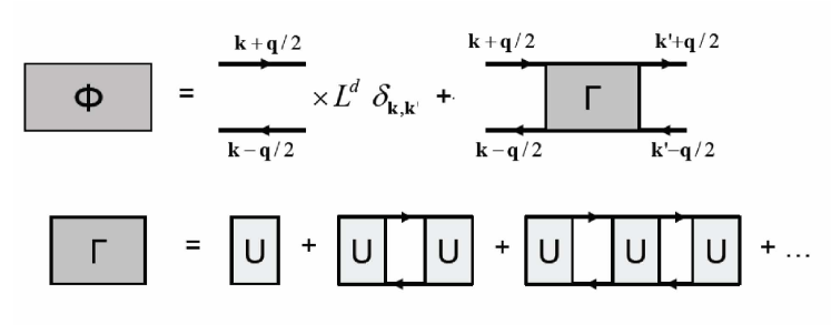
Figure 3: Relation of function $\Phi^{RA}_{\bf kk^{\prime}}({\bf q})$ with the full vertex $\Gamma^{RA}_{\bf kk^{\prime}}({\bf q})$ and the irreducible vertex $U^{RA}_{\bf kk^{\prime}}({\bf q})$.

where $P_{\bf k}({\bf q})=G^{R}_{{\bf k+q}/2}G^{A}_{{\bf k-q}/2}$ and $\Gamma^{RR}_{\bf kk^{\prime}}({\bf q})$ is omitted, since it gives no contribution due to the absence of the diffusion poles (see below). The crucial point is the presence of the factor $\Delta=1/\nu_{F}L^{d}$ before the sum over momenta in Eq.24. If vertex $\Gamma^{RA}_{\bf kk^{\prime}}({\bf q})$ is regular, then the usual rule for the change of summation by integration

$$L^{-d}\,\sum\limits_{\bf k}\,\ldots\longrightarrow\int\frac{d^{d}k}{(2\pi)^{d}}\,\ldots$$

gives a finite expression multiplied by $\Delta$, which disappears in the thermodynamic limit. In fact, vertex $\Gamma^{RA}_{\bf kk^{\prime}}({\bf q})$ contains the singular contributions related with the diffusion poles, the so called ”diffusons” and ”cooperons” (Fig. 4, a, b),

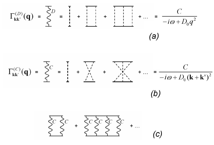
Figure 4: Definitions of the ”diffuson” (a), the ”cooperon” (b), and the cooperon ladder (c).

which give singularities $1/\omega$ for certain values of momenta. Fixation of the momentum at one value (instead of summing) gives factor $L^{-d}\propto\Delta$; if fixation of $(n-1)$ momenta allows to nullify the momentum parts in $n$ diffusion denominators, then contribution $\Delta^{n}/\omega^{n}=1/s^{n}$ appears in Eq.24, which remains finite in terms of variable $s$ when the thermodynamic limit is taken. The simplest diagram in possession of such a property is the two-cooperon one  (Fig. 4, c)

$$\Gamma^{CC}_{\bf kk^{\prime}}({\bf q})\sim L^{-d}\,\sum\limits_{{\bf k}_{1}}\frac{1}{-i\omega+D_{0}({\bf k+k_{1}})^{2}}\,\cdot$$

$$\cdot\,P_{{\bf k}_{1}}({\bf q})\,\frac{1}{-i\omega+D_{0}({\bf k}_{1}+{\bf k^{\prime}})^{2}}$$

($D_{0}$ is a classical diffusion constant). Since only the vertex with ${\bf k}={\bf k^{\prime}}$ enters in Eq.24, then fixation of momentum ${\bf k}_{1}$ at value $-{\bf k}$ nullifies the momentum parts of two diffusion denominators and gives contribution $1/s^{2}$ into $R(s)$; the same contribution is given by the diagram obtained from the two-cooperon one by reversing the lower $G$-line , so

$$R(s)=1-\frac{1}{\pi^{2}s^{2}}\,,\qquad s=\omega/\Delta\,,$$

which is a beginning of expansion over $1/s$. Contributions $1/s^{2n}$ arise, in particular, from the ladder diagrams containing $2n$ cooperons (Fig. 4, c). A summation of all such contributions should reproduce the Efetov result [25] ($x=\pi s$):

$$R(x)=1-\frac{\sin^{2}x}{x^{2}}-\left(\frac{\sin x}{x}\right)^{\prime}\int_{1}^{\infty}\frac{\sin xt}{t}\,dt\,=$$

$$=\left\{\begin{array}[]{cc}\frac{\pi}{6}x\,,&x\ll 1\\ 1-\frac{1}{x^{2}}+\frac{1+\cos^{2}x}{x^{4}}\,,&x\gg 1\end{array}\right.\,,$$

which corresponds to the Wigner-Dyson statistics. It is interesting that a summation of the cooperon ladder (Fig. 4, c) gives the result

$$R(x)=\frac{1}{\pi}\,\int_{-\infty}^{\infty}\frac{dt}{\sqrt{1+t^{2}}\sqrt{1+t^{2}+4x^{-2}}}$$

which reasonably approximates (27) (Fig. 5).

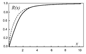
Figure 5: Comparison of the exact Efetov result (solid line) and a contribution of the cooperon ladder (dashed line).

In its improvement, the main difficulty is related with reproducing the weak oscillations, which are practically invisible in Fig. 5; the latter have the non-pertur- bative character and can be obtained only if the factorial divergency of the perturbation series is taken into account and the proper summation procedure is used [26, 27].

The analogue of the result (26) for the correlator $K(\epsilon_{1},\epsilon_{2})$ has a form [23]

$$K(\epsilon_{1},\epsilon_{2})=\frac{1}{\pi^{2}L^{2d}}\,{\rm Re}\left(\frac{1}{-i\omega+\gamma}\right)^{2}\,,$$

where $\omega=\epsilon_{1}-\epsilon_{2}$ and attenuation $\gamma$ is added, related with inelastic processes or the openness of the system . Substitution of (29) into (19) leads to expression  [23]

$$\sigma_{0}^{2}=\frac{1}{\pi^{2}}\ln\frac{E^{2}+\gamma^{2}}{\gamma^{2}}\,,$$

which coincides with Dyson’s result (14) at $\gamma\sim\Delta$. The latter fact has a following explanation. If a sufficiently large attenuation $\gamma$ is artificially introduced, then the two-cooperon contribution (29) is the main term of the expansion in $\Delta/\gamma$, and Eq.30 is substantiated. Dyson’s result (14) refers to the closed systems and implies $\gamma=0$. However, the condition of validity for (29) allows to diminish $\gamma$ only till a value of the order of $\Delta$; fortunately, the dependence on $\gamma$ is practically absent for $\gamma\mathbin{\lower 3.0pt\hbox{$\hbox to0.0pt{\raise 5.0pt\hbox{$\char 60\relax$}\hss}\mathchar 29208\relax$}}\Delta$  and result (30) is matched with Dyson’s one. Below we use the same reasoning in the more complicated case (Sec.4).

If a contribution to sum (25) is not restricted by the term ${\bf k}_{1}={-\bf k}$, but values of ${\bf k}_{1}$ close to ${-\bf k}$ are taken into account, then the following result is obtained instead of (29) [23]:

$$K(\epsilon_{1},\epsilon_{2})=\frac{1}{\pi^{2}L^{2d}}\,{\rm Re}\sum\limits_{\bf q}\left(\frac{1}{-i\omega+\gamma+D_{0}q^{2}}\right)^{2}\,.$$

The restriction by the term ${\bf q}=0$ is justified for $E\ll D_{0}/L^{2}$, while in the opposite case one can come from summation to integration and obtain for $E\gg\gamma$ [23]:

$$\sigma_{0}^{2}=\frac{1}{\pi^{2}}\sum\limits_{\bf q}\ln\left[1+\frac{E^{2}}{(\gamma+D_{0}q^{2})^{2}}\right]\,=a_{d}\left(\frac{L}{L_{E}}\right)^{d},$$

$$a_{d}=\frac{K_{d}}{\pi d\sin(\pi d/4)}\,,$$

where $L_{E}=(D_{0}/E)^{1/2}$ is the diffusion length over the time $1/E$ and $K_{d}=\left[2^{d-1}\pi^{d/2}\Gamma(d/2)\right]^{-1}$ is the surface of the unit $d$-dimensional sphere, divided by $(2\pi)^{d}$.

4. Application of Self-Consistent Theory

The next step was made by Kuchinskii and Sadov- skii [28]. Results (30, 32) are valid in the deep of the metallic phase, and one can try to extend the region of their applicability, replacing $D_{0}$ in (31) by the exact diffusion coefficient $D(\omega,q)$ [28] in the spirit of self-consistent theory of localization [5, 6]. Such approach can be motivated by the following reasoning. The irreducible vertex $U^{RA}$ (Fig. 3) contains the diffusion pole 

$$U^{RA}_{{\bf k}{\bf k}^{\prime}}({\bf q})=U_{{\bf k}{\bf k}^{\prime}}^{reg}({\bf q})+\frac{F({\bf k},{\bf k}^{\prime},{\bf q})}{-i\omega+D(\omega)({\bf k}+{\bf k}^{\prime})^{2}}\,$$

with the observable diffusion coefficient $D(\omega)$. Instead of the two-cooperon diagram (Fig. 4 c), one can consider the diagram with two blocks $U$ (Fig. 3), which dominates in the metallic phase and under certain conditions (see below) preserves domination in the general case . In the vicinity of the pole, one can put ${\bf k}^{\prime}={-\bf k}$ in the function $F({\bf k},{\bf k}^{\prime},{\bf q})$ and its role reduces to the additional factor $k_{\sigma}$ after integration over ${\bf k},{\bf q}$ in (24):

$$K(\epsilon_{1},\epsilon_{2})=\frac{k_{\sigma}\nu_{F}^{2}}{\pi^{2}}{\rm Re}\sum\limits_{\bf q}\left[\frac{\Delta}{-i\omega+D(\omega)q^{2}}\right]^{2}\,.$$

Factor $k_{\sigma}$ is a slow function of a distance to the transition, which we replace by a constant in correspondence with the accepted roughening scheme (Sec. 2).

According to [2], in a close finite system the diffusion coefficient has a localization character

$$D(\omega)=(-i\omega)\xi_{0D}^{2}\,,$$

where $\xi_{0D}$ is the correlation length of a finite system considered as quasi-zero-dimensional. Inelastic damping $\gamma$ can be introduced by replacement $-i\omega\to-i\omega+\gamma$, which is made simultaneously in the term $-i\omega$ and in $D(\omega)$ [2]. Then

$$K(\epsilon_{1},\epsilon_{2})=\frac{k_{\sigma}\nu_{F}^{2}}{\pi^{2}}\,{\rm Re}\,\frac{\Delta^{2}}{\left(-i\omega+\gamma\right)^{2}}\,F(\xi_{0D}/L)\,,$$

where function $F(x)$ is defined as

$$F(x)=\sum\limits_{\bf s}\left[\frac{1}{1+(2\pi x{\bf s})^{2}}\right]^{2}\,$$

and has the asymptotic behavior

$$F(x)=\left\{\begin{array}[]{cc}1+O(1/x^{4}),&x\gg 1\\ \tilde{c}_{d}/x^{d}\,,&x\ll 1\end{array}\right.\,;$$

Here ${\bf s}=(s_{1},\ldots,s_{d})$ is a vector with integer components $s_{i}=0,\pm 1,\pm 2\ldots$ and $\tilde{c}_{d}=\pi K_{d}(1-d/2)/2\sin(\pi d/2)$). Substitution of (36) into (19) gives

$$\sigma_{0}^{2}=\frac{k_{\sigma}}{\pi^{2}}\ln\frac{E^{2}+\gamma^{2}}{\gamma^{2}}\,F(\xi_{0D}/L)\,$$

instead of (30). We need an approximation providing a correct description in the region $\omega\sim\gamma$, which plays an essential role in the integration over $\epsilon_{1},\,\epsilon_{2}$ (see Footnote 4), and where (36) is the main term of the expansion in $\Delta/\gamma$. An example of the ladder diagrams (Fig. 4, c) shows that there exist contributions

$$\left[\frac{\Delta^{2}}{\gamma^{2}}\,F(\xi_{0D}/L)\right]^{n}$$

with all $n$, so the minimal $\gamma$ providing a validity of (36) is determined by the condition

$$\frac{\gamma_{min}^{2}}{\Delta^{2}}\,\sim\,F(\xi_{0D}/L)\,$$

and the inelastic damping cannot be diminished below this quantity. Since a dependence on $\gamma$ is practically absent for $\gamma\mathbin{\lower 3.0pt\hbox{$\hbox to0.0pt{\raise 5.0pt\hbox{$\char 60\relax$}\hss}\mathchar 29208\relax$}}\gamma_{min}$ (see below), a value of (36) at $\gamma=0$ can be estimated setting $\gamma\sim\gamma_{min}$. In proceeding to (39) one should take account of the $\omega$ dependence for $\xi_{0D}$ (Sec. 5), which effectively adds contribution $\sim E^{2}$ to the quantity $\gamma^{2}$ in the course of integration (19); hence, one should set

$$\gamma^{2}=k_{1}E^{2}+k_{2}\gamma_{min}^{2}\,,$$

where $k_{1}$ and $k_{2}$ are slowly varying functions and can be approximated by constants. As a result, we have

$$\sigma_{0}^{2}=\frac{k_{\sigma}}{\pi^{2}}\,F(\xi_{0D}/L)\ln\frac{s^{2}+k_{1}s^{2}+k_{2}\,F(\xi_{0D}/L)}{k_{1}s^{2}+k_{2}\,F(\xi_{0D}/L)}\,.$$

In moving to the deep of the localized phase, function $F(\xi_{0D}/L)$ grows to infinity and $\sigma_{0}^{2}$ tends to a constant, which accepts the Poisson value $\sigma_{P}^{2}=s$ for the choice $k_{2}=k_{\sigma}s/\pi^{2}$; so

$$\frac{\sigma_{0}^{2}}{\sigma_{P}^{2}}=u\ln\frac{1+k_{1}+u}{k_{1}+u}\,,\qquad u=\frac{k_{\sigma}}{\pi^{2}s}\,F(1/z)\,,$$

$$z=L/\xi_{0D}\,.$$

Since $\xi_{0D}/L$ is a function of $\xi/L$ [2], the scaling relation of type (7) is established for the quantity $\sigma_{0}^{2}/\sigma_{P}^{2}$.

Let discuss the sense of relation (42) and a dependence on $\gamma$ in the region $\gamma\mathbin{\lower 3.0pt\hbox{$\hbox to0.0pt{\raise 5.0pt\hbox{$\char 60\relax$}\hss}\mathchar 29208\relax$}}\gamma_{min}$. A physical interpretation of the result (32) is as follows: the system is divided into quasi-independent blocks of size $L_{E}$ [23] and the nontrivial properties of $\sigma_{0}^{2}$ are formed at the scale $L_{E}$, while for the larger scales there is addition of variances as for independent random quantities. The openness of each block provides the diffusion attenuation $\gamma_{D}=D/L_{E}^{2}=E$ of its eigenstates, with inelastic damping $\gamma$ added to it; they are combined by the law of squares, since technically it involves an estimate of $Re(-i\omega+\gamma)\sim(\omega^{2}+\gamma^{2})^{1/2}$ at $\omega\sim E$ (Sec. 5). Inelastic damping $\gamma$ is inessential in the background of $\gamma_{D}$ under condition $\gamma\mathbin{\lower 3.0pt\hbox{$\hbox to0.0pt{\raise 5.0pt\hbox{$\char 60\relax$}\hss}\mathchar 29208\relax$}}E$. It will be clear below (Sec. 5), that $\gamma_{min}\sim E$ in the critical region and $\gamma_{min}\ll E$ in the metallic one, so a dependence on $\gamma$ is absent in both regions for $\gamma\mathbin{\lower 3.0pt\hbox{$\hbox to0.0pt{\raise 5.0pt\hbox{$\char 60\relax$}\hss}\mathchar 29208\relax$}}\gamma_{min}$. In the localized regime, the scale $L_{E}$ reduces to $\xi$ and the condition $E\ll\Delta_{\xi}$ is fulfilled, where $\Delta_{\xi}$ is the level spacing for a block of size $\xi$. Under such condition, one can easily estimate the probability $p_{n}$ for existence of $n$ levels in the interval $E$ for such a block: $p_{0}\approx 1-E/\Delta_{\xi}$, $p_{1}=E/\Delta_{\xi}$, $p_{n\geq 2}\approx 0$, so $\langle N\rangle\approx E/\Delta_{\xi}$, $\langle N^{2}\rangle\approx E/\Delta_{\xi}$ and $\sigma_{0}^{2}$ is close to the Poisson value independently of the actual level statistics. Attenuation $\gamma$ can be considered as a result of the random process, which provides the scattering of each level near its average value; then independence of statistics means independence of $\gamma$. We see that a weak dependence on $\gamma$ under condition $\gamma\mathbin{\lower 3.0pt\hbox{$\hbox to0.0pt{\raise 5.0pt\hbox{$\char 60\relax$}\hss}\mathchar 29208\relax$}}\gamma_{min}$ takes place in all cases.

5. Scaling for Dynamical Conductivity and Dependence on $\omega$

In the previous section, we assumed implicitly that the quantity $\omega$ is sufficiently small. This assumption is not valid in the general case, and the $\omega$ dependence needs an additional study.

In a closed finite system, the diffusion coefficient has a localization behavior (35). In the passage to open systems, one should make a replacement $-i\omega\to-i\omega+\gamma$, and the diffusion coefficient accepts a finite value $\gamma\xi_{0D}^{2}$ in the static limit, leading to a finite conductance $g_{L}$. The scaling relations for $g_{L}$ and $\xi_{0D}$ were derived in [2] and have a form

$$g_{L}=H_{T}\left(\frac{L}{\xi_{0D}}\right)\,,\quad\pm c_{d}\left(\frac{L}{\xi}\right)^{d-2}=H\left(\frac{L}{\xi_{0D}}\right)\,,$$

where $c_{d}=\pi K_{d}/|2\sin(\pi d/2)|$ and functions $H(z)$, $H_{T}(z)$ have the asymptotic behavior

$$H(z)=\left\{\begin{array}[]{cc}\displaystyle{1/z^{2}}\,,&\qquad z\ll 1\\ -c_{d}z^{d-2}\,,&\qquad z\gg 1\end{array}\right.\,,$$

$$H_{T}(z)=\left\{\begin{array}[]{cc}\displaystyle{1/z^{2}}\,,&\qquad z\ll 1\\ \sim e^{-z},&\qquad z\gg 1\end{array}\right.\,.$$

Attenuation $\gamma_{0}$, arising due to the openness of the system, is determined by relation

$$\frac{\gamma_{0}}{\Delta}=z^{2}H_{T}\left(z\right)\,,\qquad z=L/\xi_{0D}\,,$$

so the ratio $\gamma_{0}/\Delta$ is equal to unity in the metallic phase, a somewhat less in the critical region and exponentially small in the localized state. Inelastic damping $\gamma$, which we introduce for validity of formulas, is typically much greater and $\gamma_{0}$ is inessential in its background. The above relations are valid in the limit of infinitesimal frequency and need reconsideration for finite $\omega$.

The self-consistent equation of the Vollhardt and W${\rm{\ddot{o}}}$lfle theory can be written in the form [1]

$$\frac{{\cal E}^{2}}{W^{2}}=\frac{D(\omega)}{D_{min}}+\Lambda^{2-d}\int\limits_{0}^{\Lambda}\frac{d^{d}q}{(2\pi)^{d}}\,\frac{1}{[-i\omega/D(\omega)]+q^{2}}\,$$

where ${\cal E}$ is the energy of the bandwidth order, $W$ is the random potential amplitude, $\Lambda$ is ultraviolet cut-off, $D_{min}$ is a characteristic scale of the diffusion constant, corresponding to the Mott minimal conductivity $\sigma_{min}$, and the limits of integration are indicated for the modulus of ${q}$.

For finite $L$, equation(48) accepts the following form in the closed and open systems [2]

$$\frac{{\cal E}^{2}}{W^{2}}=\frac{(-i\omega)\xi_{0D}^{2}}{D_{min}}+\Lambda^{2-d}\cdot\frac{1}{L^{d}}\sum^{(c)}_{\rm q}\,\frac{1}{q^{2}+m^{2}}\,,$$

$$\frac{{\cal E}^{2}}{W^{2}}=\frac{D_{L}(\omega)}{D_{min}}+\Lambda^{2-d}\cdot\frac{1}{L^{d}}\sum^{(o)}_{\rm q}\,\frac{1}{q^{2}+m^{2}}\,,$$

where $m^{-1}=\xi_{0D}$. Symbols $(c)$ and $(o)$ mark the allowed values of the momentum, corresponding to the closed and open systems: the main point is existence of the term with ${\bf q}=0$ in the former case and its absence in the latter [2]. The first equation determines $\xi_{0D}$, while the difference of equations defines the diffusion coefficient $D_{L}(\omega)$. Introducing the dimensionless conductance $g_{L}(\omega)=h\nu_{F}D_{L}(\omega)L^{d-2}$ and producing transformations described in [2], one obtains

$$g_{L}=\frac{p}{z^{2}}+H_{T}\left(z\right)\,,\quad\pm c_{d}\left(L/\xi\right)^{d-2}=\frac{p}{z^{2}}+H\left(z\right)\,,$$

$$p=(-i\omega+\gamma)/\Delta\,,\qquad z=L/\xi_{0D}\,,$$

where inelastic attenuation $\gamma$ is added. Now the quantity $\xi_{0D}$ depends on $\omega$ and its modulus (at $\gamma=0$) is usually denoted as $L_{\omega}$; excluding $p$, we have the scaling for dynamical conductivity

$$g_{L}(\omega)=F\left(L/\xi,L/L_{\omega}\right)\,,$$

discussed by Shapiro and Abrahams [29, 30]. Equations (51) transfer into (45) under condition $|-i\omega+\gamma|\ll\Delta$, while the opposite case is actual.

For $|p|\gg 1$, the large $z$ region is of the main interest where the second asymptotics (46) is valid for $H(z)$, while $H_{T}(z)$ is exponentially small:

$$g_{L}=\frac{p}{z^{2}}\,,\qquad\pm c_{d}\left(L/\xi\right)^{d-2}=\frac{p}{z^{2}}-c_{d}z^{d-2}\,.$$

The localized regime takes place for $z\gg|p|^{1/d}$, where

$$\xi_{0D}(\omega)=\xi_{0D}(0)\,,\quad g_{L}(\omega)=\frac{-i\omega+\gamma}{\Delta}g_{L}(0)\,,$$

and $\xi_{0D}$ does not depend on frequency, so proceeding from (36) to (39) in Sec. 4 is substantiated; the quantities $\xi_{0D}(0)$ and $g_{L}(0)$ are determined by Eqs.52 with $p=1$. If $z\ll|p|^{1/d}$, the metallic regime is realized, where

$$\xi_{0D}(\omega)=\left(\frac{-i\omega+\gamma}{\Delta}\right)^{-1/2}\xi_{0D}(0)\,,$$

$$g_{L}(\omega)=g_{L}(0)\,,$$

and the diffusion constant $D$ is frequency-independent; hence, the calculation by Altshuler and Shklovskii is adequate and equation (32) is valid with the replacement of $D_{0}$ by $D$. In the critical region ($z\sim|p|^{1/d}$) both quantities are $\omega$-dependent,

$$\xi_{0D}(\omega)\sim\left({-i\omega+\gamma}\right)^{-1/d}\,,$$

$$g_{L}(\omega)\sim\left({-i\omega+\gamma}\right)^{(d-2)/d}\,,$$

so neither (39) nor (32) is correct.

Substituting (53–55) into (36) and using the second asymptotics (38) for $F(x)$, one can write all three results in the unique form:

$$K(\epsilon_{1},\epsilon_{2})=\frac{k_{\sigma}\tilde{c}_{d}}{\pi^{2}L^{2d}}\,{\rm Re}\,\frac{1}{\left(-i\omega+\gamma\right)^{2}}\,\cdot$$

$$\cdot\,\left(\frac{-i\omega+\gamma}{\Delta}\right)^{\beta}\left[\frac{L}{\xi_{0D}(0)}\right]^{d}\,,$$

where the exponent $\beta$ accepts values $0,\,1,\,d/2$ in the localized phase, critical region and metallic state correspondingly. Equation (56) can be considered as the interpolation formula for the whole range of parameters, if $\beta$ is understood as a slowly varying function. Substituting (56) into (19) and integrating, one has

$$\sigma_{0}^{2}=\frac{2k_{\sigma}\tilde{c}_{d}}{\pi^{2}}\,{\rm Re}\,\frac{(\gamma+iE)^{\beta}-\gamma^{\beta}}{\beta(1-\beta)\Delta^{\beta}}\left[\frac{L}{\xi_{0D}(0)}\right]^{d}\,.$$

For $E\mathbin{\lower 3.0pt\hbox{$\hbox to0.0pt{\raise 5.0pt\hbox{$\char 62\relax$}\hss}\mathchar 29208\relax$}}\gamma$, the right hand side of (57) is determined by the term ${\rm Re}\,(\gamma+iE)^{\beta}\sim(\gamma^{2}+E^{2})^{\beta/2}$ and the same result by the order of magnitude follows from the expression 

$$K(\epsilon_{1},\epsilon_{2})=\frac{k_{\sigma}\tilde{c}_{d}}{\pi^{2}L^{2d}}\,{\rm Re}\,\frac{1}{\left(-i\omega+\gamma\right)^{2}}\,\cdot$$

$$\cdot\,\left(\frac{\gamma^{2}+E^{2}}{\Delta^{2}}\right)^{\beta/2}\left[\frac{L}{\xi_{0D}(0)}\right]^{d}\,.$$

It is easy to see that one can use Eq.36 with $\xi_{0D}$ independent of $\omega$, if combination $-i\omega+\gamma$ in (52) is replaced by a quantity of the order $(\gamma^{2}+E^{2})^{1/2}$; since $\gamma\sim\gamma_{min}$, it justifies representation (42) for the effective attenuation.

As a result, the second equation (52) accepts the form

$$\pm c_{d}\left(L/\xi\right)^{d-2}=\frac{s(k_{1}+u)^{1/2}}{z^{2}}-c_{d}z^{d-2}\,,$$

$$z=L/\xi_{0D}\,,$$

and together with (44) determines $\sigma_{0}^{2}$ as a function of $L/\xi$. In the critical region, one has $u\sim 1$ and $\gamma_{min}$ appears to be of the order of $E$.

6. Three-Dimensional Case

6.1. Scaling for $\sigma_{0}^{2}$

For large $s$, we can use the second asymptotics (38) for $F(1/z)$, make a replacement $u\to k_{1}u$ and exclude $z$, reducing (44), (59) to the form

$$\frac{\sigma_{0}^{2}}{\sigma_{P}^{2}}=k_{1}u\ln\frac{1+k_{1}+k_{1}u}{k_{1}+k_{1}u}\,,\qquad$$

$$\pm\left(\frac{L}{s^{1/d}\xi}\right)^{d-2}=\frac{(1+u)^{1/2}-Bu}{u^{2/d}}\,.\qquad$$

We have changed the common scale of $\xi$, in order to have the unit coefficient in the left hand side of the second equation, and introduced the parameter $B=\pi^{2}c_{d}k_{1}^{1/2}/(k_{\sigma}\tilde{c}_{d})$. Equations (60) are valid for dimensions $2<d<4$ and in the parametric form determine the scaling

$$\frac{\sigma_{0}^{2}}{\sigma_{P}^{2}}=F_{\sigma}\left(\frac{L}{s^{1/d}\xi}\right)\,,$$

so the quantities $L/\xi$ and $s$ enter only in the certain combination. Exactly such scaling was discovered in numerical experiments [11].

We can make the proper choice of parameters $k_{1}$ and $k_{\sigma}$, in order to reproduce the correct results in the metallic phase and at the critical point. Noticing that the scale $L_{E}$ coincide with $\xi_{0D}$ for $p=s$, we have $\xi_{0D}=k_{1}^{-1/4}L_{E}$ from Eq.59 in the small $z$ region; then Eq.44 gives

$$\sigma_{0}^{2}=\frac{k_{\sigma}\tilde{c}_{d}}{\pi^{2}}k_{1}^{d/4}\ln\frac{1+k_{1}}{k_{1}}\,(L/L_{E})^{d}\,,$$

which should be identified with the Altshuler and Shklovskii result (32): it gives a relation between $k_{1}$ and $k_{\sigma}$. The critical point $u_{c}$ is determined by condition $Bu_{c}=(1+u_{c})^{1/2}$ following from $\xi=\infty$, and the first equation (60) should give $\sigma_{0}^{2}/\sigma_{P}^{2}=\kappa_{0}$ for $u=u_{c}$. Considering all parameters as functions of $k_{1}$, we have a sequence of relations

$$k_{\sigma}=A_{d}\left[k_{1}^{d/4}\ln\frac{1+k_{1}}{k_{1}}\right]^{-1}\,,$$

$$B=\frac{2\pi^{2}k_{1}^{1/2}}{(d-2)k_{\sigma}}\,,$$

$$u_{c}=\frac{1+(1+4B^{2})^{1/2}}{2B^{2}}\,,$$

$$\kappa_{0}=k_{1}u_{c}\ln\frac{1/k_{1}+1+u_{c}}{1+u_{c}}\,,$$

where

$$A_{d}=\frac{4\cos(\pi d/4)}{d(1-d/2)}\,,$$

and the change of $k_{1}$ allows to adjust the correct $\kappa_{0}$ value. The actual choice of parameters for $d=3$ corresponds to $\kappa_{0}=0.28$ [11]:

$$k_{1}=0.0346\,,\quad k_{\sigma}=6.92\,,$$

$$B=0.531\,,\quad u_{c}=4.36\,.$$

The calculated dependence $y=F_{\sigma}(x)$ is presented in Fig. 6,a and compared with the numerical results [11] in Fig. 6,b.

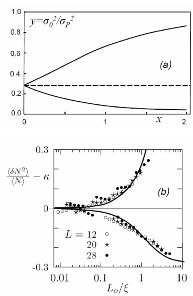
Figure 6: A theoretical dependence for $y=\sigma_{0}^{2}/\sigma_{P}^{2}$ as a function of $x=L/\xi s^{1/d}$ (a) and its comparison with numerical results of the paper [11] (b), where designation $L_{o}=Ls^{-1/3}$ was used.

6.2. Scaling for $\sigma^{2}$ and $A$.

We have established in Sec. 2 that $\sigma^{2}$ and $\sigma_{0}^{2}$ coincide in the order of magnitude. The scaling equations (60) are the same for them, and they differ only by the choice of parameters. The Poisson value for $\sigma^{2}$ is $s/2$ (see (12)) and reproduced by the choice $k_{2}=k_{\sigma}s/2\pi^{2}$, so parameter $B$ is two times less in comparison with (63). Accepting for $\sigma^{2}$ the same behavior in the metallic phase as for $\sigma_{0}^{2}$, we have instead of (63):

$$k_{\sigma}=A_{d}\left[k_{1}^{d/4}\ln\frac{1+k_{1}}{k_{1}}\right]^{-1}\,,$$

$$B=\frac{\pi^{2}k_{1}^{1/2}}{(d-2)k_{\sigma}}\,,$$

$$u_{c}=\frac{1+(1+4B^{2})^{1/2}}{2B^{2}}\,,$$

$$\kappa=\frac{1}{2}k_{1}u_{c}\ln\frac{1/k_{1}+1+u_{c}}{1+u_{c}}\,,$$

Parameter $k_{1}$ is chosen from the critical value $A_{c}=1/2\kappa=1.9$ [12] of the scaling variable $A$ (see (17)), which determines the values of other parameters:

$$k_{1}=0.0366\,,\quad k_{\sigma}=6.74\,,$$

$$B=0.280\,,\quad u_{c}=13.67\,.$$

Due to relation (17), parameter $A$ is reversal to $\sigma^{2}/\sigma_{P}^{2}$ and its scaling is trivially obtained from Eqs.60. Comparison with the Zharekeshev and Kramer data [12] is given in Fig. 7.

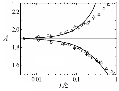
Figure 7: Numerical data by Zharekeshev and Kramer [12] for the scaling parameter $A=\sigma_{P}^{2}/\sigma^{2}$ and their comparison with a theoretical dependence.

The scaling parameter $\alpha(s_{0})$ is also determined by combination $\sigma^{2}/\sigma_{P}^{2}$, as clear from equation (16). The latter is valid for $s_{0}\gg 1$ and its extrapolation to values $s_{0}\sim 1$ cannot be reliable; so instead of $s_{0}$ some effective value $s_{eff}$ should be used.

Next, one should have in mind that for finite $s$ the quantity $\sigma^{2}/\sigma_{P}^{2}$ does not tend to zero in the metallic phase. This point can be taken into account, if the following interpolation formula is accepted for the function $F(x)$ in (37)

$$F(1/x)=1+\tilde{c}_{d}x^{d}\,,$$

which provides the correct limits (38); its substitution into (44) and (59) leads to the change in the second equation (60):

$$\pm\left(\frac{L}{s^{1/d}\xi}\right)^{d-2}=\frac{(1+u)^{1/2}-B(u-u_{0})}{(u-u_{0})^{2/d}}\,,\qquad$$

where $u_{0}\sim 1/s$. Then $u\to u_{0}$ in the metallic phase for $L\to\infty$, and $\sigma^{2}/\sigma_{P}^{2}$ tends to a finite value. If parameters for $\sigma^{2}$ are chosen in correspondence with Sec. 6.2, then the proper choice of $s_{eff}$ and $u_{0}$ allows to provide the correct values of $\alpha$ at the critical point and in the metallic region.

Scaling of parameter $\alpha(s_{0})$ was studied for $s_{0}=2$ in the paper [10] and for $s_{0}=0.473$ in the papers [11]. These results agree with the theoretical dependence, if the choice $s_{eff}=2.22$, $u_{0}=8.67$ is made in the first case (note that $s_{eff}$ is close to $s_{0}$) and $s_{eff}=2.99$, $u_{0}=10.2$ in the second case (Fig. 8). A small shift along the horizontal axis in Fig. 8,a corresponds to addition of the positive value $L_{0}$ to the length $L$, in agreement with corrections to scaling (Sec. 6.4). It should be noted, that finiteness of $u_{0}$ practically does not affect the results beyond the metallic region.

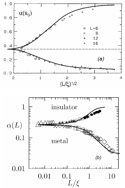
Figure 8: A theoretical dependence of $\alpha(s_{0})$ on $L/\xi$ and its comparison with numerical data of papers [10] (a) and [11] (b). Values $s_{eff}=2.22$, $u_{0}=8.67$ were used in the first case and $s_{eff}=2.99$, $u_{0}=10.2$ in the second one.

6.4. Critical Behavior and Corrections to Scaling

The simplest way to extract the critical behavior from scaling relations of type (7) is based on the possibility to rewrite them in the form ($\tau$ is a distance to the transition)

$$\alpha=F\left(\frac{L^{1/\nu}}{\xi^{1/\nu}}\right)=F\left(\tau L^{1/\nu}\right)\approx\alpha_{c}+C\tau L^{1/\nu}$$

and expand regularly over $\tau$, which is possible due to the absence of phase transitions in finite systems. Then the derivative over $\tau$ behaves as $L^{1/\nu}$ and immediately determines the critical exponent $\nu$ of the correlation length $\xi$.

Such procedure is certainly correct, if relation (7) is exact. In fact, it is not exact due to existence of scaling corrections. To analyze the latter, consider a decomposition of the sum over ${\bf q}$ in (49) suggested in [2]:

$$\frac{1}{L^{d}}\,\frac{1}{m^{2}}+\frac{1}{L^{d}}\sum\limits_{\begin{array}[]{c}{\scriptstyle{\rm q}\neq 0}\\ {\scriptstyle|{\rm q}|<\Lambda}\end{array}}\left(\,\frac{1}{m^{2}+q^{2}}-\,\frac{1}{q^{2}}\right)\,+$$

$$+\,\frac{1}{L^{d}}\sum\limits_{\begin{array}[]{c}{\scriptstyle{\rm q}\neq 0}\\ {\scriptstyle|{\rm q}|<\Lambda}\end{array}}\frac{1}{q^{2}}\,\,\equiv\,I_{1}(m)+I_{2}(m)+I_{3}(0)\,,$$

where we separated the term with ${\bf q}=0$, and rearrange the rest sum by subtraction and addition of the same sum with $m=0$. Setting ${\bf q}=2\pi{\bf s}/L$ in the second term $I_{2}(m)$, we can represent it in the form

$$I_{2}(m)=L^{2-d}H_{0}(mL)+O(m^{2}\Lambda^{d-4})\,,$$

where the first term corresponds to the limit $\Lambda\to\infty$ ($H_{0}(z)$ is a certain function), and the second gives a correction, related with finiteness of $\Lambda$. The third term in (69) can be estimated by the change of summation by integration with restriction $|q|\mathbin{\lower 3.0pt\hbox{$\hbox to0.0pt{\raise 5.0pt\hbox{$\char 62\relax$}\hss}\mathchar 29208\relax$}}1/L$

$$I_{3}(0)=\Lambda^{d-2}\left[b_{0}+b_{1}\left(\frac{a}{L}\right)^{d-2}\right]\,.$$

Then, setting $\tau={\cal E}^{2}/W^{2}-b_{0}\Lambda^{d-2}$, one has deviation of the quantity $y=\xi_{0D}/L$ from its critical value:

$$\frac{\xi_{0D}}{L}-y_{c}=C\left(\frac{L}{a}\right)^{d-2}\left[\tau+O\left(\frac{a^{2}}{\xi_{0D}^{2}}\right)\right]+O\left(\frac{a}{L}\right).$$

Differentiating over $\tau$ and resolving for $(\xi_{0D})^{\prime}_{\tau}$ in the iterational manner, one has

$$\left(\frac{\xi_{0D}}{L}\right)^{\prime}_{\tau}=C_{0}L^{d-2}+C_{1}L^{2d-6}\,.$$

In three dimensions, the main correction to scaling reduces to a constant, and for small $\tau$ we obtain

$$\frac{\xi_{0D}}{L}-y_{c}=C_{0}\tau\left(L+L_{0}\right)\,,$$

neglecting the terms disappearing at $L\to\infty$. All scaling parameters are functions of $\xi_{0D}/L$ and their deviations from critical values behave analogously.

Result (74) was obtained in [1] for other scaling parameter, while its universality was motivated by considerations based on the Wilson renormalization group. Since the results for $L$, lesser than some value $L_{min}$, always fall out of the scaling picture and are rightfully neglected by researches, dependence $L+L_{0}$ with $L_{0}>0$ can be interpreted as $L^{1/\nu}$ with $\nu>1$: such ambiguity of treatment was demonstrated in [1, 3] on a lot of examples. The results for level statistics are illustrated in Fig. 9.

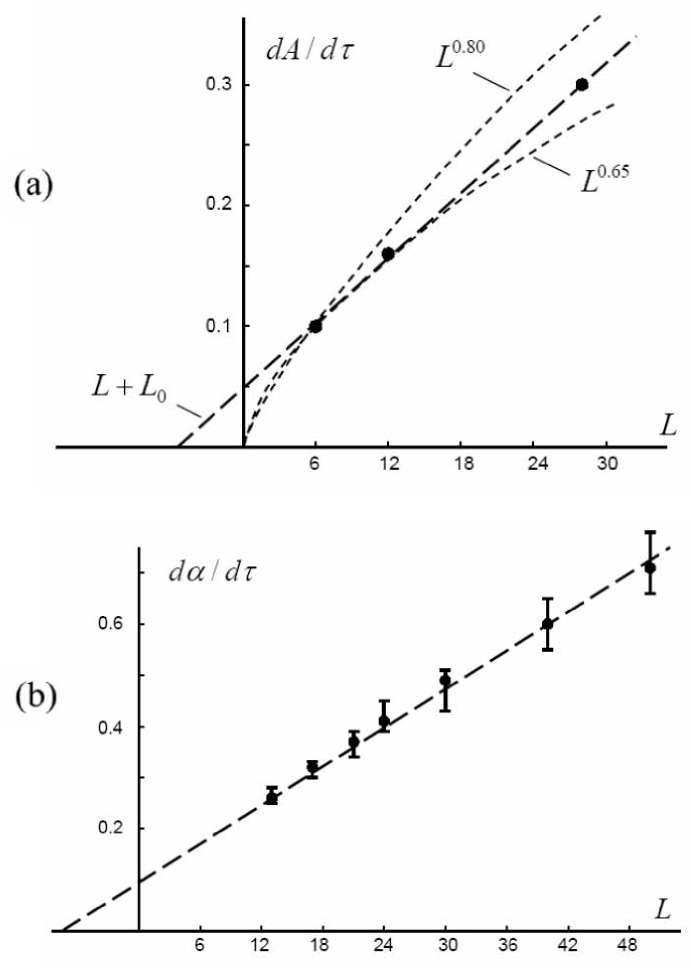
Figure 9: Fitting by dependence $(L+L_{0})$ (dashed line) for numerical data, based on the level statistics: (a) Data by Zharekeshev and Kramer [12]. The points correspond to the average derivatives of the scaling parameter $A$ (arbitrary units), determined from Fig. 4 of [12] in the interval $16<W<17$. A statistical error related with each point can be estimated very conservatively (see Table in [31]) due to the irregular character of curves given in the indicated figure; uncertainty allowed by the authors themselves corresponds to the gap between dependencies $L^{0.80}$ and $L^{0.65}$, determining the upper and lower bound of the result for the critical exponent, $\nu=1.40\pm 0.15$. (b) Data obtained by Schreiber’ group [15]; the points correspond to the derivative of the scaling parameter $\alpha$ (arbitrary units) determined by the slope of solid lines in the inset of Fig. 3 in [15]; their uncertainty is obtained by variation of the slope allowed by the size of experimental points.

7. Two-Dimensional Case

In two dimensions, the power-law function in the second equation (51) is replaced by a logarithmic one [2],

$$-c_{2}\ln\left(L/\xi\right)=\frac{p}{z^{2}}+H\left(z\right)\,,\quad c_{2}=1/2\pi$$

where asymptotics $H(z)=-c_{2}\ln z$ is sufficient for large $p$. Setting as previously $p=\left[k_{1}s^{2}+k_{2}F(1/z)\right]^{1/2}$, accepting $k_{2}=2k_{\sigma}s/\pi^{2}$ in correspondence with the Poisson condition for $\sigma^{2}$ (Sec. 6.2) and excluding $z$, one comes to the following equation

$$-\ln\left(\frac{L}{s^{1/2}\xi}\right)=B\frac{\,\,(1+u)^{1/2}}{u-u_{0}}-\ln\sqrt{u-u_{0}}$$

instead of the second equation (60). Here $u_{0}\sim 1/s$ takes into account the finiteness of $s$ in accordance with Sec. 6.3,

$$B=\frac{k_{\sigma}}{\pi^{2}k_{1}^{1/2}}=\left[\pi k_{1}\ln\frac{1+k_{1}}{k_{1}}\right]^{-1}\,,$$

and the relation between $k_{\sigma}$ and $k_{1}$ is used, obtained from the correspondence with (32). Parameter $k_{1}$ remains free and can be used as a fitting one. For large $s$, the scaling relation (61) remains valid.

In two dimensions, the more complicated scaling parameter was used [13],

$$\gamma(s_{0})={\cal N}^{-1}\int_{0}^{s_{0}}\,\left[\tilde{I}(s)-\tilde{I}_{P}(s)\right]ds\,=$$

$$={\cal N}^{-1}\int_{s_{0}}^{\infty}\,\left[I(s)-I_{P}(s)\right]ds\,,$$

where the normalization factor ${\cal N}$ is fixed by the condition that $\gamma(s_{0})=1$ for $I(s)=I_{W}(s)$. The second equality in (78) follows from the first one due to relation $I(s)=1-\tilde{I}(s)$ and the normalization of $I(s)$:

$$\int_{0}^{\infty}\,I(s)ds\,=\int_{0}^{\infty}\,sP(s)ds=\langle s\rangle=1\,.$$

For large $s_{0}$, the second integral in Eq.78 can be estimated setting $I(s)\sim\exp\{-s\sigma_{P}^{2}/\sigma^{2}\}$ (see (11)) and accepting $\sigma_{P}^{2}/\sigma^{2}$ to be practically constant,

$$\gamma(s_{0})=1-\sigma^{2}/\sigma_{P}^{2}\exp\left\{-s_{0}\frac{\sigma_{P}^{2}-\sigma^{2}}{\sigma^{2}}\right\}\,,$$

so $\gamma(s_{0})$ is determined by the quantity $\sigma^{2}/\sigma_{P}^{2}$.

In paper [13], the following dependence was empirically established for large $L/\xi$:

$$\gamma(s_{0})\sim\sigma^{2}/\sigma_{P}^{2}-1\sim(\xi/L)\,.$$

Such dependence does not take place in the present theory: it is clear from (76, 60) that $\gamma(s_{0})\sim 1/u$, $u\sim(L/\xi)^{2}$ and behavior $(\xi/L)^{2}$ is realized instead of (81). However, such law is valid practically for exponentially large values of $L/\xi$, while the numerical data are satisfactorily fitted for $k_{1}=0.002$ (Fig. 10) (a small value of $k_{1}$ is not surprising, since it was small in the $3D$ case). The reason for it is as follows: for small $k_{1}$, the large values of $u$ and $x=L/\xi s^{1/2}$ are actual, so the left and right hand sides of (76) change slowly and can be linearized near some points $u_{c}$ and $x_{c}$. A freedom in choice of the common scale of $\xi$ allows to compensate the zero term of the linear dependence and provide proportionality $u\propto L/\xi$ in the rather wide region of parameters. Thereby, dependence (81) exists really as an intermediate asymptotics.

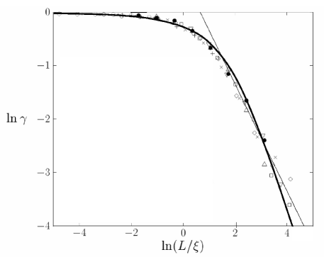
Figure 10: Numerical data of the paper [13] for $\gamma(s_{0})$ as a function of $L/\xi$ (points) in the $2D$ case and its comparison with the theoretical dependence for $k_{1}=0.002$ and $u_{0}=44$ (thick solid line); value $s_{0}=1.25$ was used in the both cases. The thin solid line corresponds to the law (81).

8. Higher Dimensions

8.1. Dimensions $d>4$

For $d>4$, one has for the quantity $I_{2}(m)$ in (69)

$$I_{2}(m)=-c_{d}m^{2}\Lambda^{d-4}\,,\qquad c_{d}=K_{d}/(d-4)$$

and the following equation is valid

$$\pm c_{d}\left(L/\xi\right)^{2}\left(L/a\right)^{d-4}=\frac{p}{z^{2}}-c_{d}z^{2}\left(L/a\right)^{d-4}$$

instead of the second equation (52). It is convenient to introduce variables

$$y=\frac{L}{\xi_{0D}}\left(\frac{L}{a}\right)^{(d-4)/4}\,,\qquad x=\frac{L}{\xi}\left(\frac{L}{a}\right)^{(d-4)/4}\,,$$

and rewrite (83) in the form

$$\pm c_{d}x^{2}=\frac{p}{y^{2}}-c_{d}y^{2}\,.$$

Setting as above $p^{2}=k_{1}s^{2}+k_{2}F(1/z)$ and choosing $k_{2}=2k_{\sigma}s/\pi^{2}$ from the Poisson value for the quantity $\sigma^{2}$ (Sec. 6.2), we have

$$\pm c_{d}x^{2}=\frac{sk_{1}^{1/2}(1+u)^{1/2}}{y^{2}}-c_{d}y^{2}\,,$$

$$u=\frac{2k_{\sigma}}{\pi^{2}k_{1}s}F(\xi_{0D}/L)\,,$$

where function $F(1/z)$ is determined by expression (37) as previously, but has a different behavior in the actual region of large $z$,

$$F(\xi_{0D}/L)=c_{d}(L/\xi_{0D})^{4}(L/a)^{d-4}=c_{d}y^{4}\,.$$

Using (87) and excluding $y$, we have instead of (60)

$$\frac{\sigma_{0}^{2}}{\sigma_{P}^{2}}=k_{1}u\ln\frac{1+k_{1}+k_{1}u}{k_{1}+k_{1}u}\,,$$

$$\pm\frac{x^{2}}{s^{1/2}}=\frac{(1+u)^{1/2}-Bu}{u^{1/2}}\,,$$

where $B=\pi^{2}k_{1}^{1/2}/2k_{\sigma}$. In the metallic phase, equations (88) give

$$\sigma^{2}=\frac{k_{1}k_{\sigma}c_{d}}{\pi^{2}}(L/L_{E})^{4}(L/a)^{d-4}\ln\frac{1+k_{1}}{k_{1}}\,,$$

which should be identified with the result for the Altshuler and Shklovskii regime

$$\sigma^{2}=\frac{c_{d}}{\pi^{2}}(L/L_{E})^{4}(L/a)^{d-4}\,,$$

which follows from (31), but does not coincide with (32). For a choice of parameters, the relations are valid

$$k_{\sigma}=\left[k_{1}\ln\frac{1+k_{1}}{k_{1}}\right]^{-1}\,,\qquad B=\frac{\pi^{2}k_{1}^{1/2}}{2k_{\sigma}}\,,$$

etc., coinciding with (66) for $d=4$.

Equations (88) define in the parametric form the following scaling relation

$$\frac{\sigma^{2}}{\sigma_{P}^{2}}=F_{\sigma}\left(\frac{x}{s^{1/4}}\right)\,,\qquad x=\frac{L}{\xi}\left(\frac{L}{a}\right)^{(d-4)/4}\,,$$

which is different from (61) and contains the atomic scale $a$. The dependence on $x\propto L^{d/4}$ instead of $L$ reduces to the change of the common scale in the logarithmic coordinates, so a construction of scaling curves can be produced in exactly the same manner as in three dimensions; however, their interpretation should be different and correspond to (92).

Let emphasize, that in higher dimensions the general form of the scaling dependence is

$$\frac{\sigma^{2}}{\sigma_{P}^{2}}=F\left(\,\frac{L}{\xi}\,,\,\frac{L}{a}\,\right)\,,$$

since the atomic scale $a$ cannot be excluded from results due to nonrenormalizability of theory [26]. At the critical point, the argument $L/\xi$ turns to zero, but a dependence on $L/a$ preserves in the general case: so the scaling parameters of the standard algorithms are usually not stationary at the critical point [1, 2]. Absence of such a dependence for the quantity $\sigma^{2}/\sigma_{P}^{2}$ (evident from (92)) is a nontrivial result of the theory, which agrees with the existence of the stationary distribution of levels established in numerical experiments [14]. It should be noted, that existence of the ”spectral rigidity” $\kappa_{0}$ was related in [18] with constancy of the conductance $g_{L}$ in the critical point. In higher dimensions, the spectral rigidity still exists, though $g_{L}$ is already not constant [2].

8.2. Four-Dimensional Case.

In four dimensions, we have for the quantity $I_{2}(m)$ in (69)

$$I_{2}(m)=-c_{4}m^{2}\ln\frac{\Lambda}{m}+O(m^{4}/\Lambda^{2})\,,\quad c_{4}=K_{4}\,$$

and come to the following equation instead of (83)

$$\pm c_{4}\left(\frac{L}{\xi}\right)^{2}\ln\frac{\xi}{a}=\frac{p}{z^{2}}-c_{4}z^{2}\ln\frac{\xi_{0D}}{a}\,,$$

which in variables

$$y=\frac{L}{\xi_{0D}}\left(\ln\frac{L}{a}\right)^{1/4}\,,\qquad x=\frac{L}{\xi}\frac{\left[\ln(\xi/a)\right]^{1/2}}{\left[\ln(L/a)\right]^{1/4}}\,$$

coincides with (85). Analogously, equation (86) is obtained with a different behavior of function $F(1/z)$ at large $z$

$$F(\xi_{0D}/L)=c_{4}(L/\xi_{0D})^{4}\ln(\xi_{0D}/a)\approx c_{4}y^{4}\,,$$

where we make use of the estimate $L\sim\xi_{0D}\gg a$ valid in the critical region. As a result, equation (88) is obtained with a different definition of $x$ and the scaling relation holds

$$\frac{\sigma^{2}}{\sigma_{P}^{2}}=F_{\sigma}\left(\frac{x}{s^{1/4}}\right)\,,\qquad x=\frac{L}{\xi}\frac{\left[\ln(\xi/a)\right]^{1/2}}{\left[\ln(L/a)\right]^{1/4}}\,$$

instead of (92). The usual scaling constructions are possible, if the quantity $\sigma^{2}/\sigma_{P}^{2}$ is considered as a function of the ”modified length” $\mu(L)=L[\ln(L/a)]^{-1/4}$.

In the metallic phase, equations (88) give

$$\sigma^{2}=\frac{k_{1}k_{\sigma}c_{4}}{\pi^{2}}\ln\frac{1+k_{1}}{k_{1}}(L/L_{E})^{4}\ln(L_{E}/a)\,,$$

while in the Altshuler and Shklovskii regime

$$\sigma^{2}=\frac{c_{4}}{\pi^{2}}(L/L_{E})^{4}\ln(L_{E}/a)\,,$$

so the previous relations (91) are valid for a choice of parameters. The actual choice corresponds to value $A_{c}=1/2\kappa=1.4$ [14]:

$$k_{1}=0.0652\,,\quad k_{\sigma}=5.49\,,$$

$$B=0.230\,,\quad u_{c}=19.9\,.$$

The main correction to scaling is determined by the term $O(m^{4}/\Lambda^{2})$ in (93), whose presence in the second equation (88) gives for $s=1$

$$b(u-u_{c})=\frac{(L/a)^{2}[\tau+c_{4}a^{4}/2\xi_{0D}^{4}]}{[\ln(\xi_{0D}/a)]^{1/2}}$$

where we have linearized the right hand side of (88) near the critical point. Differentiating over $\tau$ and resolving for $u^{\prime}_{\tau}$ in the iteration manner, one obtains for small $\tau$

$$u=u_{c}+\frac{\tau}{b}\left[\frac{(L/a)^{2})}{[\ln(L/a)]^{1/2}}+\frac{Q}{[\ln(L/a)]^{2}}\right]\,,$$

where

$$Q=\frac{\pi^{2}k_{1}}{4bk_{\sigma}}=\frac{4}{[k_{1}\ln(1/k_{1})]^{1/2}}=9.35\,.$$

In four dimensions, another scaling parameter was used [14]

$$J_{0}={\textstyle\frac{1}{2}}\langle s^{2}\rangle={\textstyle\frac{1}{2}}\int_{0}^{\infty}s^{2}P(s)\,ds=\int_{0}^{\infty}sI(s)\,ds\,.$$

It can be estimated setting $I(s)\sim\exp(-sA)$ with almost constant $A$ and taking the normalization (79) of $I(s)$ into account:

$$J_{0}\approx\left.\frac{\sigma^{2}}{\sigma_{P}^{2}}\right|_{s\sim 1}\,.$$

Such estimate is rather crude, since the integral is determined by the region $s\sim 1$, where $A$ is certainly not constant. It is more adequately to consider $J_{0}$ as a regular function of $\sigma^{2}/\sigma_{P}^{2}$, so deviations of these quantities from the critical values are proportional to each other

$$J_{0}-J_{0c}=const\,\left(\frac{\sigma^{2}}{\sigma_{P}^{2}}-2\kappa\right)\,.$$

The calculated dependence of $y=\sigma^{2}/\sigma_{P}^{2}$ on $x$ is presented in Fig. 11. If a finiteness of $s$ is taken into account, the quantity $y$ accepts a finite value in the metallic phase, and two branches of the dependence become approximately symmetric. From this point of view, the behavior of the upper branch is more representative.

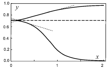
Figure 11: Calculated dependence of $y=\sigma^{2}/\sigma_{P}^{2}$ on $x$ for $d=4$. The linear portion in the interval $0.2<x<1$ is clearly seen.

For the upper branch, one can distinguish three characteristic intervals in Fig. 11: (1) region $x<0.2$ where $y-y_{c}\sim x^{2}$, corresponding to the critical behavior, (2) region $0.2<x<1$ where the dependence is practically linear, and (3) region of saturation $x>1$. The first region corresponds to rather small values of $y-y_{c}$, which are practically unattainable for numerical experiments due to their restricted accuracy . As a result, the observed dependencies (Fig. 12)

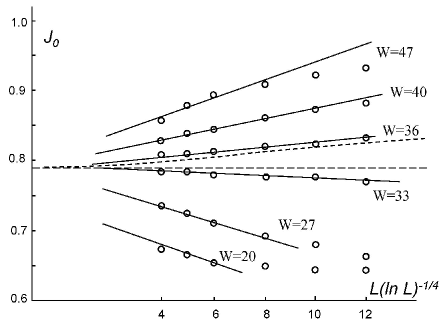
Figure 12: Numerical data for $J_{0}$ taken from Fig.4 of the paper [14] as a function of the modified length $\mu(L)=L(\ln L)^{-1/4}$ and their fitting by the linear dependence; the numbers at the horizontal axis marks the corresponding values of $L$. The dotted line is a theoretical dependence rescaled in correspondence with the slope of the linear dependence for $W=36$; to reach an agreement, the uniform shift is necessary having the order of quantity $J_{0}-J_{0c}$ at $L=4$.

are close to the linear law $y-y_{c}=c_{1}+c_{2}x$, and a small $c_{1}$ value allows to interpret them as $L^{1/\nu}$ with $\nu\approx 1$ [14]. The ratio of $c_{1}$ and $c_{2}$ is different from that in the theoretical dependence (Fig. 11), which can be explained by corrections to scaling. The main correction is given by the second term in the square brackets of Eq. 102, which is a slowly varying (almost constant) function, becoming essential for $L/a\mathbin{\lower 3.0pt\hbox{$\hbox to0.0pt{\raise 5.0pt\hbox{$\char 60\relax$}\hss}\mathchar 29208\relax$}}3$. Approximately the same uniform shift is necessary, in order to provide the correct ratio of $c_{1}$ and $c_{2}$ (Fig. 12).

9. Conclusion.

Accepting validity of self-consistent theory of localization by Vollhardt and W${\rm{\ddot{o}}}$lfle, we have derived the relations of finite-size scaling for different parameters characterizing the level statistics. A comparison with the extensive numerical material shows that on the level of raw data, the results of numerical experiments are perfectly compatible with self-consistent theory, while the opposite statements of the original papers are related with ambiguity of interpretation and existence of small parameters of the Ginzburg number type.

Small deviations, which are present in some figures, can be related with different reasons:

(a) A construction of scaling curves is related with a certain ambiguity (see the discussion in [1]). The whole scaling curve never appears in one experiment but is ”measured by pieces”. It is easy to see (Figs. 6, 7, 8, 10), that the quality of fitting can be essentially improved, if not the whole curve is treated but its separate parts.

(b) Existence of scaling corrections (Secs. 6.4, 8.2) leads to systematic distortions of the empirical scaling curves.

(c) The exploited above parameters $k_{1},\,k_{2},\,k_{\sigma}$ are in fact the slowly varying functions and their replacement by constants is unavoidable approximation related with the absence of information on these functions.

(d) In some cases, results obtained for $s_{0}\gg 1$ are extrapolated into the region $s_{0}\sim 1$.

Thereby, reasons (a,b) have a general character, while (c,d) are specific for the present paper.

In whole, we think it is possible to say on the realization of the ”minimal program”, consisting in elimination of improbably large (and violating general principles) discrepancies between the self-consistent theory and numerical experiments. As for the ”maximal program”, i.e. testing of the statement that the Vollhardt and W${\rm{\ddot{o}}}$lfle theory gives the exact critical behavior [7, 8], it needs a more detailed analysis of the existing small deviations and verification of their significance or insignificance. Such analysis is desirable for the initial raw data, and not for empirical scaling dependencies. It should be noted that in [1, 2, 3] and the present paper we have successfully described about 20 dependencies, relating to different quantities and space dimensions from 2 till 5.

References

[1] I. M. Suslov, Zh. Eksp. Teor. Fiz. 141,
122 (2012) [ JETP 114, 107 (2012)].
[2] I. M. Suslov, Zh. Eksp. Teor. Fiz. 142,
1020 (2012) [ JETP 115, 897 (2012)].
[3] I. M. Suslov, Zh. Eksp. Teor. Fiz. 142, 1230
(2012) [ JETP 1115, 1079 (2012)].
[4] P. Markos, acta physica slovaca 56, 561
(2006); cond-mat/0609580.
[5] D. Vollhardt, P. Wlfle, Phys. Rev. B 22, 4666 (1980).
[6] D. Vollhardt, P. Wlfle,
Phys. Rev. Lett. 48, 699 (1982).
[7] H. Kunz, R. Souillard, J. de Phys. Lett. 44,
L506 (1983).
[8] I. M. Suslov, Zh. Eksp. Teor. Fiz. 108,
1686 (1995) [ JETP 81, 925 (1995)].
[9] N. N. Bogoliubov and D. V. Shirkov, Introduction to the
Theory of Quantized Fields (Nauka, Moscow, 1976;
Wiley, New York, 1980).
[10] B. I. Shklovskii, B. Shapiro, B. R. Sears et al,
Phys. Rev. B 47, 11487 (1993).
[11] I. Kh. Zharekeshev, B. Kramer, in ”Quantum Dynamics
in Submicron Structures”, Ed. by H. Cerdeira et al
(NATO ASI Series, North-Holland, Kluwer Academic Publishers)
Ser. E, 291, 93 (1995);
I. Kh. Zharekeshev, Vestn. Evraziiskogo Nats. Univ. 77,
41 (2010).
[12] I. Kh. Zharekeshev, B. Kramer, Phys. Rev. Lett. 79, 717 (1997).
[13] I. Kh. Zharekeshev, M. Batsch, B. Kramer,
Europhys. Lett. 34, 587 (1996).
[14] I. Kh. Zharekeshev, B. Kramer, Ann. Phys.
(Leipzig) 7, 442 (1998).
[15] F. Milde, R. A. Romer, M. Schreiber,
Phys. Rev. B 61, 6028 (2000).
[16] A. MacKinnon, B. Kramer, Phys. Rev. Lett. 47,
1546 (1981); Z. Phys. 53, 1 (1983).
[17] K. Slevin, T. Ohtsuki, Phys. Rev. Lett. 82, 382
(1999).
[18] B. L. Altshuler, I. Kh. Zharekeshev, S. A.
Kotochigova, B. I. Shklovskii, Zh. Eksp. Teor. Fiz.
94, 343 (1988) [Sov. Phys. JETP 67, 625 (1988)].
[19] F. J. Dyson, J. Math. Phys. 3, 140, 157,
166 (1962).
[20] G. Korn and T. Korn, Mathematical Handbook for
Scientists and Engineers (McGraw-Hill, New York, 1968;
Nauka, Moscow, 1977).
[21] E. Abrahams, P. W. Anderson, D. C. Licciardello, and
T. V. Ramakrishman, Phys. Rev. Lett. 42, 673 (1979).
[22] V. P. Chistyakov, Course of the Probability
Theory, Moscow, Nauka, 1982.
[23] B. L. Altshuler, B. I. Shklovskii, Zh. Eksp. Teor.
Fiz. 91, 220 (1986) [Sov. Phys. JETP 64, 127 (1986)].
[24] L. N. Bulaevskii, M. V. Sadovskii,
Pis’ma Zh. Eksp. Teor. Fiz. 43, 76 (1986)
[JETP Letters, 43, 99 (1986)].
[25] K. B. Efetov, Zh. Eksp. Teor. Fiz.
83, 833 (1982) [Sov. Phys. JETP 56, 467 (1982)].
[26] I. M. Suslov, Usp. Fiz. Nauk 168, 503 (1998)
[Physics – Uspekhi 41, 441 (1998)].
[27] I. M. Suslov, Zh. Eksp. Teor. Fiz. 127, 1350
(2005) [ JETP 100, 1188 (2005)].
[28] E. Z. Kuchinskii, M. V. Sadovskii,
Zh. Eksp. Teor. Fiz. 98, 634 (1990)
[Sov. Phys. JETP 71, 354 (1990)].
[29] B. Shapiro, E. Abrahams, Phys. Rev. B 24,
4889 (1981).