BI-TP 2014/04
arXiv:1402.5302v2
June 2014

Finite size dependence of scaling functions of the
three-dimensional $O(4)$ model in an external field
J. Engels^a and F. Karsch^a,b

^a Fakultät für Physik, Universität Bielefeld, D-33615 Bielefeld, Germany

^b Physics Department Brookhaven National Laboratory, Upton, NY 11973

Abstract

We calculate universal finite-size scaling functions for the order parameter and the longitudinal susceptibility of the three-dimensional $O(4)$ model. The phase transition of this model is supposed to be in the same universality class as the chiral transition of two-flavor QCD. The scaling functions serve as a testing device for QCD simulations on small lattices, where, for example, pseudocritical temperatures are difficult to determine. In addition, we have improved the infinite-volume limit parametrization of the scaling functions by using newly generated high statistics data for the $3d$ $O(4)$ model in the high temperature region on an $L=120$ lattice.

PACS : 64.10.+h; 75.10.Hk; 05.50+q

Keywords: Scaling function; $3d$ $O(4)$ model; finite size scaling; universality

 
E-mail addresses: engels@physik.uni-bielefeld.de, karsch@physik.uni-bielefeld.de, karsch@bnl.gov

1 Introduction

The three-dimensional $O(4)$ spin model plays an important role for our understanding of the low energy limit of Quantumchromodynamics (QCD) as well as its phase structure at non-zero temperature. The almost massless pseudo-scalar particles (pions) of QCD have been considered already early as Goldstone particles, which receive a non-zero mass only due to the presence of a chiral symmetry breaking field, i.e. the non-zero light quark masses. The consequences of this idea for the QCD phase diagram have been worked out in detail in a paper by Pisarski and Wilczek [1]. Their conclusion is that, if QCD undergoes a second-order chiral transition in the limit of vanishing up and down quark masses, this transition is expected to belong to the universality class of the three-dimensional $O(4)$ spin model . Thermodynamics in the vicinity of the QCD transition will then show universal features that are described by $O(4)$ scaling functions. In fact, recent studies of the quark mass dependence of the chiral transition in lattice QCD using the staggered fermion discretization scheme led to good agreement with infinite-volume $O(2)$ or $O(4)$ scaling functions [2].

Lattice QCD calculations with light dynamical quarks are performed in relatively small volumes. This is in particular the case for the computationally demanding chiral fermion formulations, i.e., for studies of QCD thermodynamics performed with domain wall fermions [3] or overlap fermions [4]. A finite volume limits the correlation length and thus, similar to the influence of an external field, it modifies the universal behavior in the vicinity of a second-order phase transition. It has been shown that the finite volume dependence of the chiral condensate close to the QCD transition temperature may be understood in terms of finite-volume scaling functions of the $3d$ $O(4)$ spin model [5].

Calculations performed within the framework of an $O(4)$ symmetric quark-meson model, using an approximation scheme based on the functional renormalization group (FRG) approach [6, 7], suggest as well that finite size effects may influence the determination of the chiral transition temperature, or more generally, the temperature dependence of the chiral susceptibility in QCD. It thus is of interest to arrive at quantitative results for the finite size dependence of the scaling functions of the $3d$ $O(4)$ universality class which can be used in scaling studies of thermodynamic observables determined in lattice QCD. Within the FRG approach [8] these scaling functions have been derived approximately (In Ref. [8] the exponent $\eta$ is zero, unlike in the $O(4)$ class.).

In a recent paper [9], we had derived representations of the scaling functions of the $3d$ $O(4)$ model in the thermodynamic limit. This was done in terms of expansions of the scaling functions in the scaling variable $z=\bar{t}/h^{1/\Delta}$, where $\Delta=\beta\delta$ is the so-called gap exponent and $h=H/H_{0}$ and $\bar{t}=(T-T_{c})/T_{0}$ are the reduced field and temperature. The parameters of the expansions were deduced exclusively from Monte Carlo data with finite external fields. In the paper [9] we discussed in detail the relations, the common features and the differences of the new parametrization to the existing, previous ones, which nearly all used the Widom-Griffiths form [10, 11], where both the scaling function and the scaling variable depend on the magnetization $M\,$. We had also derived in Ref. [9] the corresponding parametrization of the scaling function $f_{f}(z)$ for the singular part of the free energy density. The scaling functions $f_{G}(z)$ and $f_{\chi}(z)$ of the magnetization and the susceptibility are obtained from $f_{f}(z)$ by taking appropriate derivatives with respect to $H$.

In this paper we will determine finite-volume scaling functions of the order parameter and the susceptibility directly from high statistics Monte Carlo simulations of the $3d$ $O(4)$ spin model for varying $L$ and finite external field. The paper is thus a direct extension of Ref. [9] to finite $L$ for a limited region of $z$. For further details which are not dependent on $L$ being finite one should therefore consult Ref. [9]. As far as we know, the only other study of finite-size scaling relations in the presence of an external field for the $3d$ $O(4)$ spin model is that of Ref. [5]. In that paper, however, the finite-size scaling relations were examined only for two fixed values of $z$, namely for $z=0$ and $z=z_{p}$, that is at the critical temperature and on the pseudocritical line, whereas we cover a larger region in $z$.

Our paper is organized as follows. In section 2 we extend the relations for the infinite-volume scaling functions to the case of finite $L=V^{1/d}$. The simulations of the $3d$ $O(4)$ model on lattices with $L=24-120$ and the resulting finite volume dependencies of the scaling functions $f_{G}$ and $f_{\chi}$ are then discussed in section 3. In addition we improve the parametrization of the infinite-volume scaling functions as given in Ref. [9]. We close with a summary and the conclusions.

2 Finite size dependence of scaling functions

In order to introduce the finite size dependence of the scaling functions we reconsider parts of chapter 2 of Ref. [9]. The scaling functions are derived from the reduced (containing a factor ${\beta=1/T}$ ) free energy density,

$$f=-\frac{1}{V}\ln Z(T,H,L)=f_{s}(T,H,L)+f_{ns}(T,H,L)\ .$$ (1)

Here, we have split the free energy density in a singular term $f_{s}$, responsible according to renormalization group (RG) theory for critical behavior, and a regular or non-singular term $f_{ns}$. The scaling laws near the critical point are derived from the RG scaling equation for $f_{s}$. The derivatives of $f_{ns}$ contribute regular terms to the scaling laws, which apart from the cases of the energy density and the specific heat (for $\alpha<0$) are sub-leading near the critical point. The dependence on $L$ or better on $1/L$ can be treated as a correction to leading scaling behavior, that is $l=L_{0}/L$ takes the rôle of an additional relevant scaling field with exponent $y_{L}=1$. The RG equation becomes then

$$f_{s}(u_{t},u_{h},l,u_{4},\dots)=b^{-d}f_{s}(b^{y_{t}}u_{t},b^{y_{h}}u_{h},b\,l,b^{y_{4}}u_{4},\dots)\ .$$ (2)

Here, $b$ is a free positive scale factor and the usual, remaining relevant scaling fields are $u_{t}=c_{t}t$, $u_{h}=c_{h}H$, where $t=(T-T_{c})/T_{c}$. The $c_{t},c_{h}$ and $L_{0}$ are model-dependent (positive) metric scale factors. In addition, there are infinitely many irrelevant scaling fields $u_{j}$ with negative exponents $y_{j}$. By choosing $b=u_{h}^{-1/y_{h}}$ for $H>0$ one obtains from Eq. (2) the form of scaling functions which we want to discuss here

$$f_{s}(u_{t},u_{h},l,u_{j>3})=u_{h}^{d/y_{h}}f_{s}(u_{t}u_{h}^{-y_{t}/y_{h}},1,l\,u_{h}^{-1/y_{h}},u_{j}u_{h}^{-y_{j}/y_{h}})~{}.$$ (3)

The dependence of $f_{s}$ on the irrelevant scaling fields leads to the non-analytic corrections to the scaling functions and is here of the form

$$u_{j}u_{h}^{-y_{j}/y_{h}}=u_{j}(c_{h}H)^{-y_{j}/y_{h}},$$ (4)

and not $\sim L^{y_{j}}$ as in the conventional approach where one chooses $b\sim L$. Hence, we only have a single variable, $lu_{h}^{-1/y_{h}}$, that depends on $L$ and all other variables are $L$-independent. Close to the critical point, when $H$ is small, the contributions of the irrelevant scaling fields become negligible, because the $y_{j}$ are negative. The singular term $f_{s}$ is then a universal function of the scaling fields $u_{t},u_{h}$ and $l$ only and

$$f_{s}\;=\;(c_{h}H)^{d/y_{h}}\Psi_{2}(c_{t}c_{h}^{-y_{t}/y_{h}}tH^{-y_{t}/y_{h}},c_{h}^{-1/y_{h}}l\,H^{-1/y_{h}})~{},$$ (5)

where $\Psi_{2}$ is again a universal function but in contrast to the thermodynamic limit now of two arguments. By comparison with the infinite-volume scaling laws one derives

$$y_{t}\;=\;1/\nu\;,\;y_{h}\;=\;1/\nu_{c}\;=\;\Delta/\nu\;,\;{\rm or~{}}\;\Delta\;=\;y_{h}/y_{t}~{},$$ (6)

and the known hyperscaling relations between the critical exponents.

Instead of working with the metric scale factors $c_{t}$ and $c_{h}$ one introduces usually new temperature and field variables $\bar{t}=tT_{c}/T_{0}$ and $h=H/H_{0}$ in the thermodynamic limit. We stick to this tradition also in the finite volume case. Correspondingly, the scaling functions of the observables which are derivatives of the free energy density will depend (see Eq. (5)) on the two variables

$$z=\bar{t}/h^{1/\Delta}~{},\quad{\rm and}\quad z_{L}=l/h^{\nu_{c}}~{},$$ (7)

and the thermodynamic limit is recovered for $z_{L}=0$ at finite $h$. For example, the order parameter, or magnetization becomes then

$$M=-\frac{\partial f}{\partial H}=h^{1/\delta}f_{G}(z,z_{L})\ .$$ (8)

In order to specify the scaling variables $z$ and $z_{L}$ in a given model calculation one needs to fix the non-universal scales $T_{0}$, $H_{0}$ and $L_{0}$. As already mentioned, the first two are fixed by demanding in the infinite volume limit

$$M(t=0)=h^{1/\delta}\;\;{\rm and}\;\;M(h=0)=(-t)^{\beta}\;.$$ (9)

This implies

$$f_{G}(0,0)\;=\;1~{},\quad{\rm and}\quad f_{G}(z,0){\raisebox{-4.30554pt}{$\stackrel{{\scriptstyle\displaystyle\longrightarrow}}{{\scriptstyle z\rightarrow-\infty}}$}}(-z)^{\beta}~{}.$$ (10)

The scale $L_{0}$ is fixed by a third normalization condition. We choose

$$z_{L}=1\;\;{\rm for}\;\;\frac{M(t=0)_{|L}}{M(t=0)_{|L=\infty}}=f_{G}(0,1)=0.874\;.$$ (11)

That is, on a given lattice of size $V=L^{d}$ we determine at $t=0$ the finite-volume scaling function $f_{G}(0,z_{L})$ by varying the external field $h$. We then assign the value $z_{L}=1$ to that value of $h$ that yields $f_{G}(0,1)=0.874$. This fixes the scale $L_{0}$ to be $L_{0}=Lh^{\nu_{c}}$. Our normalization condition seems arbitrary. In fact, we could have chosen other normalization conditions. However, in the absence of any obvious natural choice the above normalization condition is convenient. As we shall see this condition leads to $L_{0}\equiv 1$ for the $3d$ $O(4)$ spin model studied here.

Due to Eq. (5) and the derivative in Eq. (8) the singular term $f_{s}$ depends on the scaling function $f_{f}(z,z_{L})$

$$f_{s}=H_{0}h^{1+1/\delta}f_{f}(z,z_{L})\ ,$$ (12)

which relates to $f_{G}$ by

$$f_{G}(z,z_{L})=-\left(1+\frac{1}{\delta}\right)f_{f}(z,z_{L})+\frac{z}{\Delta}\frac{\partial f_{f}(z,z_{L})}{\partial z}+\nu_{c}z_{L}\frac{\partial f_{f}(z,z_{L})}{\partial z_{L}}\ .$$ (13)

Fluctuations of the order parameter in the $O(4)$ model, are described by the longitudinal susceptibility,

$$\chi_{L}={\partial M\over\partial H}={h^{1/\delta-1}\over H_{0}}f_{\chi}(z,z_{L})~{},$$ (14)

with

$$f_{\chi}(z,z_{L})={1\over\delta}f_{G}(z,z_{L})-\frac{z}{\Delta}\frac{\partial f_{G}(z,z_{L})}{\partial z}-\nu_{c}z_{L}\frac{\partial f_{G}(z,z_{L})}{\partial z_{L}}~{}.$$ (15)

A further observable of interest is the thermal susceptibility $\chi_{t}$, the mixed second derivative of $f$,

$$\chi_{t}={\partial M\over\partial(1/T)}=-\frac{T^{2}}{T_{0}}h^{(\beta-1)/\Delta}\;\frac{\partial f_{G}(z,z_{L})}{\partial z}~{}.$$ (16)

Both $\chi_{L}$ and $\chi_{t}$ have their counterparts in QCD.

We note that our finite-size scaling functions relate in a simple way to the ones that are commonly used in the literature [5, 8]. In terms of these functions our observables read

$$M\;\; = \;\;L^{-\beta/\nu}Q_{G}(z,z_{L})~{},$$ (17)

$$\chi_{L}\;\; = \;\;\frac{L^{\gamma/\nu}}{H_{0}}Q_{\chi}(z,z_{L})~{},$$ (18)

$$\chi_{t}\;\; = \;\;\frac{T^{2}}{T_{0}}L^{-(\beta-1)/\nu}Q_{t}(z,z_{L})~{},$$ (19)

and the connection to our scaling functions is

$$Q_{G}(z,z_{L})\;\; = \;\;(z_{L}/L_{0})^{-\beta/\nu}f_{G}(z,z_{L})~{},$$ (20)

$$Q_{\chi}(z,z_{L})\;\; = \;\;(z_{L}/L_{0})^{\gamma/\nu}f_{\chi}(z,z_{L})~{},$$ (21)

$$Q_{t}(z,z_{L})\;\; = \;\;(z_{L}/L_{0})^{-(\beta-1)/\nu}\left(-\frac{\partial f_{G}(z,z_{L})}{\partial z}\right)~{}.$$ (22)

Of particular interest for the determination of the infinite-volume scaling functions is the leading (in $L$) or asymptotic form of the $Q$-functions [5]. One obtains for $L\rightarrow\infty$

$$Q_{G}\rightarrow f_{G}(z,0)(hL^{1/\nu_{c}})^{1/\delta}~{},\quad Q_{\chi}\rightarrow f_{\chi}(z,0)(hL^{1/\nu_{c}})^{1/\delta-1}~{},$$ (23)

$$Q_{t}\rightarrow-\frac{\partial f_{G}(z,0)}{\partial z}(hL^{1/\nu_{c}})^{(\beta-1)/\Delta}~{},$$ (24)

that is, at fixed $z$ we have powers of $hL^{1/\nu_{c}}$ with infinite-volume scaling functions as coefficients.

3 Simulation of the 3$d$ $O(4)$ model

We determine the finite-size scaling functions from simulations of the standard $O(4)$-invariant nonlinear $\sigma$-model. It is defined by

$$\beta\,{\cal H}\;=\;-J\,\sum_{<{\vec{x}},{\vec{y}}>}\vec{\phi}_{\vec{x}}\cdot\vec{\phi}_{\vec{y}}\;-\;{\vec{H}}\cdot\,\sum_{{\vec{x}}}\vec{\phi}_{\vec{x}}\;,$$ (25)

where ${\vec{x}}$ and ${\vec{y}}$ are nearest-neighbor sites on a three-dimensional hyper-cubic lattice, $\vec{\phi}_{\vec{x}}$ is a four-component unit vector at site ${\vec{x}}$. The coupling $J$ and the external field $\vec{H}$ are reduced quantities, that is they contain already a factor $\beta=1/T$. That allows us to consider the coupling directly as the inverse temperature, $J\equiv 1/T$. An additional factor on $J$ would just change the scale of $T$. The setup of our calculations and the definition of further observables are given in detail in Ref. [9]. There are two differences to the simulations in Ref. [12], which we used in [9] to calculate the infinite-volume scaling functions $f(z)\equiv f(z,0)\,$. Instead of calculating at fixed $T$ and varying $H$, we fix $z$ and vary $H$ and secondly we use, according to the average clustersize, an appropriate number of cluster updates such as to cover before each measurement the whole volume $V$ of the lattice 5 to 6 times. That becomes relevant in particular with increasing $z>0$ and leads there to much better statistics. For example, on a lattice of size $L=120$ we made between 400 (at $z=0.1$) and 14.000 cluster updates (at $z=4.0$) for each of our 100.000 measurements. In order to define our variables $t,\bar{t},h$ and $z$, we use the same critical amplitudes, temperature and exponent values for the $3d$ $O(4)$ model as in Refs. [12] and [13]. These are

$$J_{c}=0.9359(1),\,\,T_{0}=1.093(18),\,\,H_{0}=4.845(66),\,\,\beta=0.380(2),\,\,\delta=4.824(9)~{}.$$ (26)

From the hyperscaling relations one obtains then

$$\nu=0.7377(41)~{},\quad\gamma=1.4531(104)~{},\quad\Delta=1.8331(103)~{},\quad\nu_{c}=0.4024(2)~{}.$$ (27)

The exponents $\beta$ and $\delta$ were deduced exclusively from Monte Carlo data for the magnetization at finite external fields. In Ref. [14] the spontaneous magnetization on the coexistence line, that is for $T<T_{c}$ and $H=0$, was determined by extrapolating at fixed $T$ from finite fields to $H=0$, exploiting the Goldstone behavior. We wanted to convince ourselves that the value of $\beta$ in Eq. (26) is still in agreement with the high statistics data for the $3d$ $O(4)$ model that had been produced on a lattice with $L=120$ at finite $H$ and $J=0.95,0.97,1.0$ and 1.2 for Ref. [12]. We have extrapolated these data also to $H=0$ in order to improve and to complement the data of Ref. [14]. With the complete data set we have made various fits of the form

$$M(T,H=0)=b_{M}(T_{c}-T)^{\beta}(1+b_{M1}(T_{c}-T)^{\theta})~{},$$ (28)

with and without the correction-to-scaling factor, where $\theta=0.574$ was taken from Table 3 of the paper [15] by Guida and Zinn-Justin. A free fit with corrections resulted in $\beta=0.379(4)$, negligible correction amplitude $b_{M1}=0.0007(228)$ and $\chi^{2}/N_{f}=1.13$. An even better fit was obtained without corrections, $b_{M1}\equiv 0$, with $\chi^{2}/N_{f}=0.85$ and $\beta=0.3792(2)$. Further fits, varying e. g. $T_{c}$ slightly, or omitting the point closest to $T_{c}$ in the fits, led us to our error estimate for $\beta$ in Eq. (26). Our $\beta$-value differs from the value $\beta=0.388(1)$ derived from the exponents $\eta$ and $\nu$ which were determined by Hasenbusch [16] at vanishing external fields on small lattices. A fit to our data with fixed $\beta=0.388$ without corrections is practically excluded, because then $\chi^{2}/N_{f}=263.5$ and half of the data are outside the fit curve. Including a correction factor a reasonable fit with $\chi^{2}/N_{f}=2.44$ is possible, though at the expense of a noticeable correction amplitude $b_{M1}=-0.0514(22)$. That however, contradicts another, well-known result of Ref. [16]: the leading correction-to-scaling amplitude of the $3d$ $O(4)$ nonlinear $\sigma$-model is essentially zero. That is exactly what we found here and in Ref. [9], it was found as well in Ref. [13], where $\delta$ was determined, and confirmed again by Ref. [17]. We note, that our set of exponents has been used as well in the successful determination of the scaling functions of the transverse and even longitudinal (for $z>0$) correlation lengths [12, 13]. The exponents, also our $\nu$-value, are thus consistent with the data.

The main goal of our simulations was, as already explained, to study the finite size dependence of the scaling functions $f_{G}$ and $f_{\chi}$. We have done this by calculating the scaling functions at fixed $z$ and varying $z_{L}=l/h^{\nu_{c}}$. Here, lattices of size $L=24,36,48,72,96$ and external fields $H$ in the range $[0.0005,0.003]$ have been used, supplemented at some $z$-values by results from $L=120$ lattices. The upper limit of the $H$-range, 0.003, was chosen much smaller than that of Ref. [5], 0.10, to suppress correction terms $\sim H^{\omega\nu_{c}}$. Here, $-\omega=y_{4}$ is the largest irrelevant exponent. The $z$-range that we have considered is $[-1.0,2.0]$, that is, we cover the region around the critical point and the high temperature region up to and including the peak area of $f_{\chi}(z,0)\,$. In Ref. [9] we had determined the peak position to $z_{p}=1.374(30)$. It defines the pseudocritical line $z=z_{p}$ in the $(t,h)$-plane where $\chi_{L}$ is at its maximum for fixed $h$ and varying $t$.

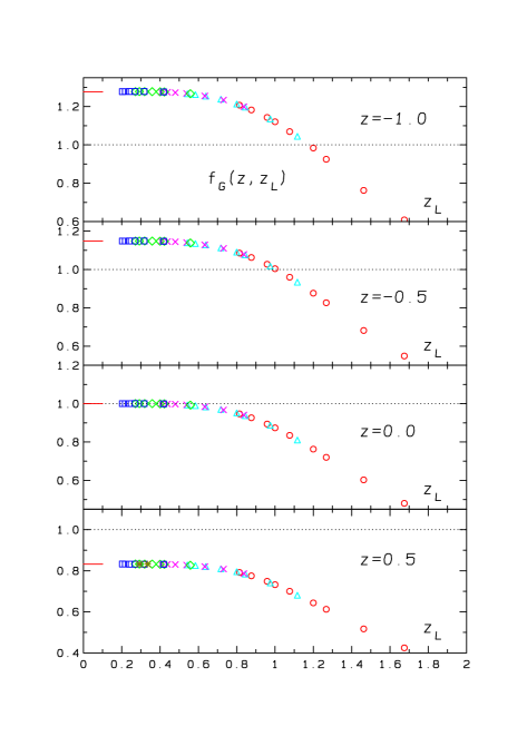
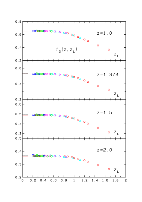
Figure 1: The finite-volume scaling function $f_{G}(z,z_{L})$ for some values of $z$ versus $z_{L}$. For each value of $z$ lattices of size $L=24$ (circles), 36 (triangles), 48 (crosses), 72 (diamonds), 96 (squares) and various values of $h$ have been used. For $z=0.5,1.0,1.5$ and $2.0$ also data for $L=120$ (stars) have been added. Short horizontal lines close to $z_{L}=0$ show the values of the infinite-volume scaling function $f_{G}(z)$, the solid lines denote the new parametrization, the dashed lines the one of Ref. [9].

All our results for the scaling function $f_{G}(z,z_{L})$ are summarized in Fig. 1. In order to plot the data as a function of $z_{L}=L_{0}/Lh^{\nu_{c}}$ we have fixed $L_{0}=1$. As can be seen in the $(z=0)$-part of the plot that amounts to the normalization condition Eq. (11). In Fig. 2 we have used the same data to show the $z$-dependence of $f_{G}(z,z_{L})$ at fixed $z_{L}$-values. We see from the two figures that finite size effects in the scaling function $f_{G}$ are small for $z_{L}\leq 0.5$. The main effects appear in the low temperature region and decrease with increasing $z$. This is in particular evident from Fig. 2 .

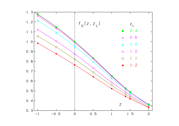
Figure 2: The finite-volume scaling function $f_{G}(z,z_{L})$ for some values of $z_{L}$ versus $z$. Curves shown are spline interpolations of the data, the points for $z_{L}=0.4$ are not connected, the highest line shows $f_{G}(z,0)$ from the new parametrization.

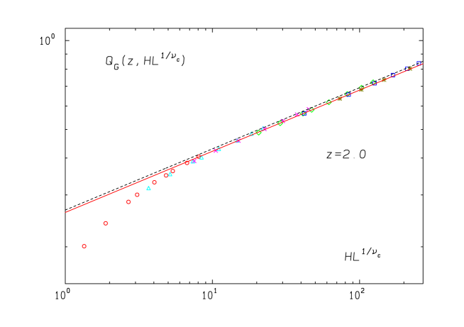
Figure 3: The finite-volume scaling function $Q_{G}$ for $z=2$ versus $HL^{1/\nu_{c}}$. The lines show the asymptotic forms, Eq. (23), calculated from $f_{G}(z)$ using the parametrizations of Ref. [9] (dashed line) and the one given in Appendix A (solid line).

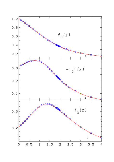
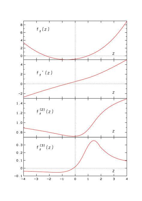
Figure 4: Left part: The infinite-volume scaling functions $f_{G}(z),\,-f_{G}^{\prime}(z)$ and $f_{\chi}(z)$ for $z>0$, $T>T_{c}$ from data (circles) for $M,\chi_{t}$ and $\chi_{L}$ on an $L=120$ lattice. The lines are from the parametrization of the scaling functions in Appendix A. Right part: The scaling function $f_{f}(z)$ and its first three derivatives from the new parametrization.

Another important observation is that we find perfect finite size scaling in $z_{L}$ for $z\leq 1.0$. That means, at fixed $z$, $f_{G}$ is de facto only a function of $z_{L}$ and there is no further significant dependence $\sim H^{\omega\nu_{c}}$. At larger values of $z$, however, the results from different size lattices start to deviate from each other. In addition, the data at fixed $z$ do no longer reach a plateau for $z_{L}\rightarrow 0$, even for the same lattice size. Obviously, one needs here data on larger lattices and/or smaller $H$-values. The effect is known from Ref. [5], where the scaling functions $Q_{G}$ had been calculated for $z=0$ and $z=z_{p}$. In Fig. 4 of Ref. [5], $Q_{G}(z_{p})$ is shown as a function of $HL^{1/\nu_{c}}$, instead of $z_{L}$. One observes, that with increasing $H$ the corresponding data at fixed $L$ overshoot the asymptotic result and this happens the earlier the smaller $L$ is. Only for small $H$ and large $L$ there is a small window, where we have coincidence with the asymptotic behavior expected from Eq. (23). In fact, also our parametrization from Ref. [9], which was based on results from lattices with $L=120$, is apparently affected by the use of data with too large field values in the peak region. In order to check this we have made a logarithmic plot of the scaling function $Q_{G}=ML^{\beta/\nu}$ at $z=2$ versus $HL^{1/\nu_{c}}$ with our new high statistics data. As is clearly seen in Fig. 3, the asymptotic form of $Q_{G}$ predicted by the parametrization in Ref. [9] is slightly too high at $z=2$. In order to remedy the deficiencies we had had in parametrizing the infinite-volume scaling functions for $z>0$ in Ref. [9], namely too low statistics, too high field values and no systematic covering of the necessary $z$-range, we decided to produce new high statistics data on an $L=120$ lattice at fixed $z$-values with two or three low field values. These new data are shown in Fig. 4 for $f_{G}(z),-f_{G}^{\prime}(z)$ and $f_{\chi}(z)$ together with a new parametrization, whose details we list in Appendix A. The new data cover now in particular the peaks with sufficient accuracy. In Figs. 1 and 2 we have already displayed the infinite volume values for $f_{G}$ close to $z_{L}=0$. We see that a difference to the old parametrization is here only visible for $z\raise 1.29167pt\hbox{$>$\kern-7.5pt\raise-4.73611pt\hbox{$\sim$}}1$. In the right part of Fig. 4 we show the scaling function of the free energy density and its first three derivatives. Our results for the finite-volume scaling function of the susceptibility are shown in Figs. 5 and 6. We see again the strongest finite size effects for the smaller values of $z$. In particular, the peak of the susceptibility is washed out completely on small lattices or large $z_{L}$, so that there a pseudocritical temperature cannot be determined safely. We note, that the peak position of $f_{\chi}(z,0)$ has shifted slightly to $z_{p}=1.35(3)$ due to the new parametrization. The value is, however, inside the error bars of the old value $z_{p}=1.374(30)$.

$a_{nm}$		n
		0	1	2	3	4
	3	0.0421332	-0.0782771	0.0546495	-0.0251385	0.0017542
	4	0.0576183	0.3302893	-0.2642637	0.0617961	0.0049618
m	5	-0.6352819	-0.3461722	0.4678005	-0.0453606	-0.0309722
	6	0.5355251	0.1770113	-0.3118316	0.0061252	0.0295072
	7	-0.1247180	-0.0369583	0.0696270	0.0021488	-0.0078913

Table 1: Expansion coefficients

In Figs. 2 and 6 we have shown spline interpolations of our data. When using the scaling functions in the analysis of data for other models, it may be more convenient to use polynomial interpolation formulas. We have fitted simultaneously all our data for $f_{G}(z,z_{L})$ and $f_{\chi}(z,z_{L})$ to a polynomial ansatz for $f_{G}(z,z_{L})$,

$$f_{G}(z,z_{L})=f_{G}(z,0)+\sum_{n=0}^{4}\sum_{m=3}^{7}a_{nm}z^{n}z_{L}^{m}\;.$$ (29)

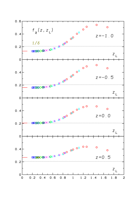
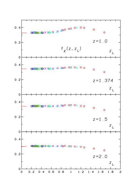
Figure 5: The finite-volume scaling function $f_{\chi}(z,z_{L})$ for some values of $z$ versus $z_{L}$. For each value of $z$ lattices of size $L=24$-$96$ and various values of $h$ have been used. For $z=0.5,1.0,1.5$ and $2.0$ we have also added results from lattices of size $L=120$. The notation for the symbols is as in Fig. 1 . The infinite volume predictions for $f_{\chi}$ are shown as short horizontal lines.

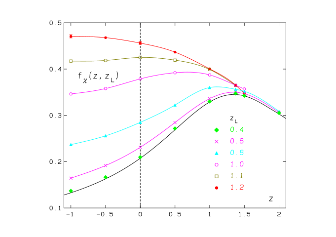
Figure 6: The finite-volume scaling function $f_{\chi}(z,z_{L})$ for some values of $z_{L}$ versus $z$. Curves shown are spline interpolations of the data, the points for $z_{L}=0.4$ are not connected, the lowest line shows $f_{\chi}(z,0)$ from the new parametrization.

We use here of course the new parametrization of the infinite-volume scaling function $f_{G}(z,0)$ as discussed in Appendix A. The ansatz for $f_{\chi}(z,z_{L})$ is obtained from $f_{G}(z,z_{L})$ using Eq. (15). We obtained the expansion coefficients $a_{nm}$ from a simultaneous fit to data for $f_{G}(z,z_{L})$ and $f_{\chi}(z,z_{L})$. As can be seen in Figs. 1 and 5 in the interval $z\in[-1.0,2.0]$ significant finite size effects in $f_{G}$ and $f_{\chi}$ only set in for $z_{L}\geq 0.5$. For this reason we use in Eq. (29) a polynomial ansatz that starts with finite volume corrections at ${\cal O}(z_{L}^{3})$. That is, the leading corrections are proportional to $1/L^{3}$. We also performed fits with smaller powers of $z_{L}$ which, however, did not improve over the current ansatz. Results for the expansion coefficients $a_{nm}$ are given in Table 1. This parametrization is appropriate for $f_{G}$ and $f_{\chi}$ in the intervals $z\in[-1.0,2.0]$ and $z_{L}\in[0.0,1.2]$.

4 Summary and conclusions

In our paper we have investigated the finite-size scaling functions of the universality class of the $3d$ $O(4)$ spin model. Our aim was to provide a suitable form for tests on this universality class of QCD data, which were obtained from simulations on small lattices. In contrast to the commonly studied finite-size scaling functions $Q_{G}$ [5], $Q_{\chi}$ and so forth, we have directly extended the infinite-volume scaling functions to finite-size scaling functions $f(z,z_{L})$, which describe the size dependence as well. The $z$-region, where we have examined these functions, encompasses the vicinity of the critical point and the high temperature region up to and including the peak area of $f_{\chi}(z,0)$. Thereby, we cover the domain where the pseudocritical line obtained from the susceptibility is of interest. In order to actually use the finite-size scaling functions for a test of a model, one has, of course, to determine the four model specific parameters $T_{c},T_{0},H_{0}$ and $L_{0}$.

We have seen from Figs. 1 and 2 for $f_{G}(z,z_{L})$ and Figs. 5 and 6 for $f_{\chi}(z,z_{L})$ that on one hand finite size effects are small for $z_{L}<0.5$ and on the other hand that the main finite size effects appear in the small $z$-region and that they decrease with increasing $z$. In the course of our analysis we found out that the parametrization of the infinite-volume scaling function $f_{G}(z)$ as given in Ref. [9] had to be improved in the region $z\geq 1.0$ . We have therefore generated new high statistics data on an $L=120$ lattice at fixed $z$ in the range $[0.1,4.0]$ at several small field values each. These data enabled us to update the parametrization [9]. Its results are presented in Appendix A. The expansion coefficients given in Table 1 are based on the new parametrization of the infinite-volume scaling function.

As a by-product of our calculations we obtained new values for the universal product $R_{\chi}=d_{0}^{+}=1.0919(14)$ and the universal ratio $A^{+}/A^{-}=1.734(75)$. Also the peak positions of $f_{\chi}$ and $-f_{G}^{\prime}$ changed slightly to $z_{p,\chi}=1.35(3)$ and $z_{p,t}=0.78(4)$, respectively.

Acknowledgment

This work has been supported in part by contract DE-AC02-98CH10886 with the U.S. Department of Energy.

Appendix A Update on the infinite volume form of
the scaling function $f_{G}$

As already shown in Section 3, Fig.  4, we have new data for $z>0$. We have used these data and those of Ref. [9] for $z\leq 0$ to update the parametrization in [9] of the infinite-volume scaling functions. We started with the Taylor series around $z=0$

$$f_{G}(z)\;=\;\sum_{n=0}^{\infty}b_{n}z^{n}~{}.$$ (30)

Like in [9], we have fitted the data from $-f_{G}^{\prime}(z)$ for small $z$. Here, this was done once in the $z$-range $[-2.5,1.0]$ up to $n=7$, and once in the range $[-0.5,2.3]$ up to $n=8$ but with the coefficients $b_{0},\dots,b_{4}$ from the first fit as input. The results of the first fit are to be used for $z\leq 0$, the others for $z>0$. The coincidence of the lowest coefficients guarantees smooth fits at $z=0$ for all the derivatives we need. The final result for the coefficients is

$$b_{0}\equiv 1~{},~{}~{}b_{1}=-0.316123\pm 0.000628~{},~{}~{}b_{2}=-0.0418371\pm 0.000661~{},$$ (31)

$$b_{3}=~{}0.00129543\pm 0.000859~{},~{}~{}b_{4}=~{}0.00582947\pm 0.000345~{}.$$ (32)

The remaining coefficients are different for $z<0$ and $z>0$. We find for $z>0$

$$b_{5}^{+}=~{}0.00201377\pm 0.000887~{},~{}~{}b_{6}^{+}=~{}0.0048998\pm 0.001122~{},$$ (33)

$$b_{7}^{+}=-0.00386218\pm 0.000484~{},~{}~{}b_{8}^{+}=~{}0.00068511\pm 0.000071~{},$$ (34)

and for $z<0$

$$b_{5}^{-}=~{}0.00257848\pm 0.000450~{},~{}~{}b_{6}^{-}=~{}0.00053247\pm 0.000211~{},$$ (35)

$$b_{7}^{-}=~{}0.000044801\pm 0.000030~{}.$$ (36)

We next consider the asymptotic expansions. In the high temperature region, that is for $z\rightarrow\infty$, or for $t>0$ and $h\rightarrow 0$, we use the ansatz

$$f_{G}(z)\;=\;z^{-\gamma}\cdot\sum_{n=0}^{\infty}d_{n}^{+}z^{-2n\Delta}~{}.$$ (37)

In the low temperature region, for $t<0$ and $h\rightarrow 0$, we make the following ansatz for $f_{G}(z)$

$$f_{G}(z)\;=\;(-z)^{\beta}\cdot\sum_{n=0}^{\infty}d_{n}^{-}(-z)^{-n\Delta/2}~{}.$$ (38)

We have fitted $f_{G}$ in the positive $z$-range $[1.5,4]$ with the first four terms of Eq. (37) and found

$$d_{0}^{+}=1.09185\pm 0.00137~{},~{}~{}d_{1}^{+}=-1.48536\pm 0.03995~{},$$ (39)

$$d_{2}^{+}=3.24559\pm 0.3619~{},~{}~{}d_{3}^{+}=-3.65645\pm 0.9676~{}.$$ (40)

For negative $z$ we retain the result of the three-term, asymptotic fit from [9]

$$d_{0}^{-}\equiv 1~{},~{}~{}d_{1}^{-}=0.273651\pm 0.002933~{},~{}~{}d_{2}^{-}=0.0036058\pm 0.004875~{}.$$ (41)

The approximations for the small $z$ and asymptotic expansions, described above, overlap for both $z>0$ and $z<0$ in large $z$-ranges. For $z>0$ we change from the small $z$ to the asymptotic fits at $z=1.85$, for $z<0$ at $z=-2.0$. Now everything is fixed and we can calculate the coefficients of the leading asymptotic terms of $f_{f}(z)$ from Eqs. (59) and (62) of Ref. [9]. We find

$$c_{0}^{+}=0.417756382\pm 0.00656~{},~{}~{}c_{0}^{-}=0.240933670\pm 0.00913~{}.$$ (42)

From the last equation one obtains a new estimate of the universal ratio,

$$\frac{A^{+}}{A^{-}}=1.734\pm 0.075~{}.$$ (43)

The new result for the ratio is slightly lower than the results $1.842(43)$ from [9], the estimates found in Refs. [18], $1.91(10)$, and [19], $1.8(2)$, but still in agreement within the error bars, though our error estimate does not include the systematic error due to a possible variation of the critical exponents used.

References

- [1] R. D. Pisarski and F. Wilczek, Phys. Rev. D 29, 338 (1984).
- [2] S. Ejiri et al., Phys. Rev. D 80, 094505 (2009) [arXiv:0909.5122 [hep-lat]].
- [3] A. Bazavov et al. [HotQCD Collaboration], Phys. Rev. D 86, 094503 (2012) [arXiv:1205.3535 [hep-lat]].
- [4] G. Cossu, S. Aoki, H. Fukaya, S. Hashimoto, T. Kaneko, H. Matsufuru and J.-I. Noaki, Phys. Rev. D 87, 114514 (2013) [arXiv:1304.6145 [hep-lat]].
- [5] J. Engels, S. Holtmann, T. Mendes and T. Schulze, Phys. Lett. B 514, 299 (2001) [hep-lat/0105028].
- [6] J. Braun, B. Klein and P. Piasecki, Eur. Phys. J. C 71, 1576 (2011) [arXiv:1008.2155 [hep-ph]].
- [7] J. Braun, B. Klein and B.-J. Schaefer, Phys. Lett. B 713, 216 (2012) [arXiv:1110.0849 [hep-ph]].
- [8] J. Braun and B. Klein, Eur. Phys. J. C 63, 443 (2009) [arXiv:0810.0857 [hep-ph]].
- [9] J. Engels and F. Karsch, Phys. Rev. D 85, 094506 (2012) [arXiv:1105.0584 [hep-lat]].
- [10] B. Widom, J. Chem. Phys. 43, 3898 (1965).
- [11] R. B. Griffiths, Phys. Rev. 158, 176 (1967).
- [12] J. Engels and O. Vogt, Nucl. Phys. B 832, 538 (2010) [arXiv:0911.1939[hep-lat]].
- [13] J. Engels, L. Fromme and M. Seniuch, Nucl. Phys. B 675, 533 (2003) [hep-lat/0307032].
- [14] J. Engels and T. Mendes, Nucl. Phys. B 572, 289 (2000) [hep-lat/9911028].
- [15] R. Guida and J. Zinn-Justin, J. Phys. A 31, 8103 (1998) [cond-mat/9803240].
- [16] M. Hasenbusch, J. Phys. A 34, 8221 (2001) [arXiv:cond-mat/0010463].
- [17] M. Hasenbusch and E. Vicari, Phys. Rev. B 84, 125136 (2011) [arXiv:1108.0491[cond-mat]].
- [18] F. Parisen Toldin, A. Pelissetto and E. Vicari, JHEP 07, 029 (2003) [arXiv:hep-ph/0305264].
- [19] A. Cucchieri and T. Mendes, J. Phys. A 38, 4561 (2005) [hep-lat/0406005].