Short Gamma Ray Burst Formation Rate from BATSE data using $E_{p}-L_{p}$ correlation and the minimum gravitational wave event rate of coalescing compact binary

Abstract

Using 72 Short Gamma Ray Bursts (SGRBs) with well determined spectral data observed by BATSE, we determine their redshift and the luminosity by applying $E_{p}$–$L_{p}$ correlation for SGRBs found by Tsutsui et al. (2013). For 53 SGRBs with the observed flux brighter than $4\times 10^{-6}~{}{\rm erg~{}cm^{-2}s^{-1}}$, the cumulative redshift distribution up to $z=1$ agrees well with that of 22 Swift SGRBs. This suggests that the redshift determination by the $E_{p}$–$L_{p}$ correlation for SGRBs works well. The minimum event rate at $z=0$ is estimated as $\rho_{SGRB}(0)=6.3_{-3.9}^{+3.1}\times 10^{-10}~{}{\rm events~{}Mpc^{-3}yr^{-1}}$ so that the minimum beaming angle is $0.6^{\circ}-7.8^{\circ}$ assuming the merging rate of $10^{-7}-4\times 10^{-6}~{}{\rm events~{}Mpc^{-3}yr^{-1}}$ suggested from the binary pulsar data. Interestingly, this angle is consistent with that for SGRB130603B of $\sim 4^{\circ}-8^{\circ}$(Fong et al., 2014). On the other hand, if we assume the beaming angle of $\sim 6^{\circ}$ suggested from four SGRBs with the observed value of beaming angle, the minimum event rate including off-axis SGRBs is estimated as $\rho_{SGRB,all}^{min}(0)=1.15_{-0.71}^{+0.57}\times 10^{-7}~{}{\rm events~{}Mpc^{-3}yr^{-1}}$. If SGRBs are induced by coalescence of binary neutron stars (NSs) and/or black holes (BHs), this event rate leads to the minimum gravitational-wave detection rate of $\rm 3.9_{-2.4}^{+1.9}(152_{-94}^{+75})~{}events~{}y^{-1}$ for NS-NS (NS-BH) binary, respectively, by a worldwide network with KAGRA, advanced-LIGO, advanced-Virgo, and GEO.

1. Introduction

Although the number of observed Short Gamma-Ray Bursts (SGRBs) is increasing, their central engine is still a big mystery. A major candidate is coalescence of compact objects such as neutron stars and stellar-mass black holes. One of the keys to confirm this idea is the formation rate of SGRBs as a function of redshift. In fact, if SGRBs are truly induced by coalescence of compact objects, the SGRB formation rate will track the star formation rate with some delay time. Further, if this is the case, SGRBs are expected to be accompanied by substantial gravitational-wave emission. Thus, the local SGRB formation rate is directly related to the expected number of gravitational-wave events for the next-generation gravitational-wave detectors such as KAGRA , advanced-LIGO , advanced-VIRGO and GEO .

However, the number of SGRBs with known redshift is very small ($\sim 20$) so that the formation rate is not easy to estimate. Previous studies have estimated the formation rate assuming the functional form of the formation rate and the luminosity function and fitting the data to derive model parameters (Guetta & Piran, 2005, 2006; Nakar, Gal-Yam & Fox, 2006; Dietz, 2011; Metzger & Berger, 2012; Petrillo, Dietz & Cavaglia, 2013). In this approach, the result depends on the functional form of the model and has large statistical errors due to the small number of SGRBs used to fit the model.

On the other hand, as to Long Gamma-Ray Bursts (LGRBs), the formation rate has been estimated much more precisely and robustly. This is because the correlation between the spectral peak energy and luminosity was found and used to estimate the redshift of LGRBs without known redshift. First, Yonetoku et al. (2004) analyzed data of 16 LGRBs observed by CGRO BATSE and BeppoSAX with known redshifts, and found the $E_{p}-L_{p}$ correlation between the $E_{p}$ and the peak luminosity $L_{p}$ integrated for 1 s time interval at the peak as,

$$L_{p}=\rm 2.34\times 10^{51}erg~{}s^{-1}(\frac{E_{p}}{100keV})^{2}.$$ (1)

The linear correlation coefficient of the $\log E_{p}-\log L_{p}$ correlation is 0.958 and the chance probability is $5.31\times 10^{-9}$. Then Ghirlanda et al. (2005a, b); Krimm et al. (2009); Yonetoku et al. (2010) checked the properties of the correlation and confirmed its reliability. Using this correlation, Yonetoku et al. (2004) estimated the redshift for 689 bright BATSE LGRBs without known redshift and derived the luminosity function and the formation rate.

As to SGRBs, however, due to the small number of the events with known redshifts and the good spectra to determine $E_{p}$, it has been difficult to do a similar analysis. Recently, Tsutsui et al. (2013) succeeded in determining $E_{p}-L_{p}$ correlation for SGRBs. They used 8 secure SGRBs out of 13 candidates and obtained

$$L_{p}=\rm 7.5\times 10^{50}erg~{}s^{-1}(\frac{E_{p}}{100keV})^{1.59},$$ (2)

where $E_{p}$ is from the time integrated spectrum again while $L_{p}$ was taken as the luminosity integrated for 64 ms time intervals at the peak considering the shorter duration of SGRB. The linear correlation coefficient of the $E_{p}-L_{p}$ correlation is 0.98 and the chance probability is $1.5\times 10^{-5}$. Although this is not so tight as that for LGRBs due to the fact that the number of SGRBs is half of that of LGRBs, it is accurate enough to use as a redshift indicator for many SGRB events without known redshifts.

In this article, we determine the redshifts of SGRBs observed by BATSE using the $E_{p}$–$L_{p}$ correlation mentioned above. Then, we obtain a non-parametric estimate of the luminosity function and SGRB formation rate versus redshift based on much more samples compared with previous studies. This article is organized as follows. In §2 , we describe the observations and data analyses. After that, we show the redshifts estimated by $E_{p}$–$L_{p}$ correlation for SGRBs, and obtain the cumulative redshift distribution and compare it with the observed one. We also show the cumulative luminosity function and the SGRB formation rate as a function of redshift with non-parametric method, i.e. without any assumptions on both distributions. §3 is devoted to discussions and implications of the results.

2. Observations & Data Analyses

2.1. Data Selection

We used the BATSE current burst catalog which contains 2704 GRBs during its life time ($\sim 9.2$ years) in orbit. The average fraction of sky coverage of BATSE instruments is 0.483, so the effective life time is $\sim 4.4$ years for the entire sky. We selected events with the short time duration of $T_{90}<2$ sec in the observer frame as SGRB candidates. Here $T_{90}$ is measured as the duration of the time interval during which 90 % of the total observed counts have been detected. After that, we selected the brightest 100 SGRBs in 1,024 ms peak photon flux. The peak flux of all events we selected is brighter than $1~{}{\rm photons~{}cm^{-2}s^{-1}}$. The trigger efficiency of BATSE instrument is almost 100 % (larger than 99.988 %), so we can estimate SGRB rate without any correction in this point.

2.2. Spectral Analyses

We used spectral data detected by the BATSE LAD detectors and performed the standard data reduction method. Then we succeeded in analyzing spectral data for 72 events. The other 28 events are statistically poor or the variable background condition, so we failed to obtain spectral parameters for the standard analyses.

We used the spectral model of the smoothly broken power-law model, so called Band function (Band et al., 1993) as following;

$$N(E)=\left\{\begin{array}[]{ll}A\Bigl{(}\frac{E}{100~{}{\rm keV}}\Bigr{)}^{\alpha}\exp(-\frac{E}{E_{0}})\\ {\rm for}\ E\leq(\alpha-\beta)E_{0},\\ A\Bigl{(}\frac{E}{100~{}{\rm keV}}\Bigr{)}^{\beta}\Bigl{(}\frac{(\alpha-\beta)E_{0}}{100~{}{\rm keV}}\Bigr{)}^{\alpha-\beta}\exp(\beta-\alpha)\\ {\rm for}\ E\geq(\alpha-\beta)E_{0},\end{array}\right.$$ (7)

where, $N(E)$ is in unit of $\rm{photons~{}cm^{-2}s^{-1}keV^{-1}}$. The spectral parameters of $\alpha$, $\beta$ and $E_{0}$ is the low- and high-energy index, and the energy at the spectral break, respectively. For the case of $\beta<-2$ and $\alpha>-2$, the peak energy can be derived as $E_{p}=(2+\alpha)E_{0}$. In previous work, although Ghirlanda et al. (2009) performed spectral analyses for 79 SGRBs with cutoff power-law model, we used the Band function for all events in this work because the $E_{p}$–$L_{p}$ correlation by Tsutsui et al. (2013) is based on the Band function. If we can not determine the high energy spectral index $\beta$, we fixed the parameter as $\beta=-2.25$ which is average value of bright events.

2.3. Redshift Estimation for SGRBs

For long GRBs, there are well known correlations between $E_{p}$ and brightness like Amati – Yonetoku – Ghirlanda correlations (e.g. Amati et al., 2002; Yonetoku et al., 2004; Amati, 2006; Ghirlanda et al., 2004; Yonetoku et al., 2010). Recently Tsutsui et al. (2013) reported the $E_{p}$–luminosity correlation in SGRBs as equation 2. This is $\sim 5$ times dimmer than the $E_{p}$–luminosity correlation of long GRBs (see equation 1). This equation can be rewritten as

$$\frac{d_{L}^{2}}{(1+z)^{1.59}}=\frac{10^{50.88}}{4\pi F_{p}}\Bigl{(}\frac{E_{p}}{100~{}{\rm keV}}\Bigr{)}^{1.59}~{}~{}~{}{\rm erg~{}s^{-1}}.$$ (8)

Here, the right side of the equation is composed by observed values. As Yonetoku et al. (2004) performed, using the observed $E_{p}$ and 64 msec peak flux, we can estimate the pseudo redshift and luminosity distance for each event. Then we used the cosmological parameters of $\Omega_{m}=0.3$, $\Omega_{\Lambda}=0.7$ and Hubble parameters of $H_{0}=71~{}{\rm km~{}s^{-1}Mpc^{-1}}$.

We succeeded in calculating all pseudo redshifts for 72 events. In figure 1, we show the data distribution on the plane of redshift and 64ms peak luminosity. The filled squares and circles are known redshift samples with precious spectral parameters (secure SGRBs by Tsutsui et al., 2013) and pseudo redshift samples, respectively. The error of pseudo redshift is mainly caused by the statistical uncertainty of $E_{p}$, and the one of luminosity depends on the estimated redshift. The solid line is caused by the flux limit which must pass just close to the lowest and the highest data point because of a demand of our method to estimate the SGRB rate and luminosity function. If not, there is a possibility that the algorithm recognize unmeaning stronger luminosity evolution because of the lack of data around the flux limit. In this analyses, we set the flux limit of $4\times 10^{-6}~{}{\rm erg~{}cm^{-2}s^{-1}}$ to hold the number of data as many as possible.

In figure 2, we show the correlation between the $E_{p}$ value of this work (Band function) and the ones of Ghirlanda et al. (2009) (cutoff power-law function: CPL). We confirmed both results strongly correlate with each other while our $E_{p}$ is slightly smaller than their results. This result is recognized as the difference of model function as Kaneko et al. (2006) mentioned. The cutoff power-law tends to have larger $E_{p}$ than the Band function.

To confirm if our redshift determination is consistent with one of the known redshift SGRBs, we compared the cumulative redshift distributions of both samples. In figure 3, we show the cumulative redshift distribution of 22 observed SGRBs of $z\leq 1.13$ (red) (fong13a) and our 45 BATSE SGRBs brighter than the flux limit and with the pseudo redshift of $z\leq 1.14$ (black) in figure 1, respectively. The reason we set upper bound of the redshift comes from the small number (only one) of the known redshift SGRB larger than $z=1.13$.

We performed the Kolmogorv-Smirnov test between the red and black lines in figure 3, and it shows the probability of null-hypothesis is 79.4 %. Moreover we estimate possible error region of the cumulative distribution of 45 pseudo redshift samples. As shown in figure 1, the estimated redshifts have errors mainly come from $E_{p}$ errors, so we performed 100 Monte Carlo simulations for each point and estimated their cumulative redshift distributions. The results are also shown as gray lines in figure 3, and we can see the error region well contains the observed distribution (red line). Therefore we conclude our estimated redshift distribution is the almost same distribution of observed one, and the $E_{p}$–$L_{p}$ correlation for SGRBs (Tsutsui et al., 2013) is a good distance indicator. Hereafter we use 53 SGRBs above the flux truncation of $4\times 10^{-6}~{}{\rm erg~{}cm^{-2}s^{-1}}$ with maximum redshift $z=2.2$ to estimate the SGRB formation rate in the next section.

2.4. Methodology

In general, luminosity function can be written as $\Psi(L,z)=\rho(z)\phi(L/g_{k}(z),\alpha_{s})/g_{k}(z)$. Here we named $\rho(z)$, $\phi(L/g_{k}(z),\alpha_{s})$, and $g_{k}(z)$ are the SGRB formation rate, the local luminosity function, and the luminosity evolution, respectively. The parameter $\alpha_{s}$ means the shape of luminosity function, but we ignore this effect because of the limited number of samples. The goal of this analysis is to estimate the SGRB rate $\rho$ as a function of only $z$, and the local luminosity function $\phi(L/g_{k}(z))$ after removing the luminosity evolution effect.

The statistical problem to estimate the true SGRB formation rate and luminosity functions is how to deal the data set truncated by the flux limit. In many cases, assuming some parametric forms (model functions) for the luminosity function and redshift distribution, all parameters are simultaneously estimated to fit the data distribution of the flux limited samples. However, if we use the model function far from the true distribution, we may obtain unrealistic solutions for each parameters. Especially, we have little knowledge about the functional form of SGRB formation rate and it may be different from the general star formation rate. Therefore it is preferable to use a non-parametric method.

In this paper, we used a non-parametric method by Lynden-Bell (1971); Efron & Petrosian (1992); Petrosian (1993); Maloney & Petrosian (1999) developed to estimate the redshift distribution of distant Quasars. This method is also used in the long GRBs (e.g. Lloyd-Ronning, Petrosian & Mallozzi, 2001; Yonetoku et al., 2004; Dainotti, Petrosian, Singal et al., 2014). The details of methodologies are found in these papers so that we briefly summarized the thread of data analyses to estimate the luminosity function and the SGRB formation rate independently. In this work we follow the notations and terminologies by Yonetoku et al. (2004) to identify the best luminosity function distribution of $\Psi(L,z)$; see their section 4.

2.5. SGRB Formation Rate

First of all, we estimate the correlation between the redshift and the luminosity (luminosity evolution) with the assumption of the functional form of $g_{k}(z)=(1+z)^{k}$. Then we searched the appropriate $k$-value which gives the data distribution on $(z,L/g_{k}(z))$ plane has no correlation between them. Then we calculated the $\tau$-statistical value (similar to Kendall $\tau$ rank correlation coefficient) to measure the correlation degree for the flux truncated data. When the $\tau$ value is zero, it means that the combined luminosity $L/g_{k}(z)$ is independent of the redshift $z$ (no luminosity evolution). We estimated $k=3.3^{+1.7}_{-3.7}$ with 1 $\sigma$ uncertainty, so we can say there is no obvious luminosity evolution ($g_{k}(z)\equiv 1$).

Next, we can separately calculate the local luminosity function for $L/g_{k}(z)$, i.e. $L$ for $g_{k}(z)=1$, and the SGRB formation rate as a function of redshift with non-parametric method. We have already removed the effect of luminosity evolution, a unique formula for the luminosity function can be adopted for all redshift range. Then, we can easily estimate the number of events lower than the flux limit. In the same way, we can also estimate the SGRB formation rate.

In figure 4, we show the cumulative luminosity function of $L/g_{k}(z)$. The red line is the best estimate with the pseudo redshift, and gray lines are results by 100 Monte Carlo simulations as previously shown. For long GRBs, several authors reported the luminosity function can be described as broken power-law (e.g. Yonetoku et al., 2004). However, in this analysis for SGRBs, we can not find obvious break structure in figure 4. We adopt a simple power-law function, and obtained the best fit index of $-0.84_{-0.09}^{+0.07}$ between the luminosity range of $10^{51}$ and $10^{53}~{}{\rm erg~{}s^{-1}}$. We can say the luminosity function is consistent with the pure unbroken power-law for $L>10^{50}~{}{\rm erg~{}s^{-1}}$.

In figure 5, we show the SGRB formation rate per comoving volume and the proper time as a function of $(1+z)$. Again, the red line is the best estimate with the pseudo redshift, and gray lines are results by 100 Monte Carlo simulations. Here, we used the BATSE’s effective observation period of 4.4 years as already explained in section 2.1. This SGRB rate is calculated for the events with the peak luminosity of $L>10^{50}~{}{\rm erg~{}s^{-1}}$ in observer’s frame. The functional form can be described as

$$\rho_{\rm SGRB}(z)\propto\left\{\begin{array}[]{ll}(1+z)^{6.0\pm 1.7}&{\rm for}~{}(1+z)<1.67,\\ {\rm const.}&{\rm for}~{}(1+z)\geq 1.67,\end{array}\right.$$ (11)

in units of ${\rm events~{}Mpc^{-3}yr^{-1}}$. The local minimum event rate at $z=0$ is $\rho_{\rm SGRB}(0)=6.3_{-3.9}^{+3.1}\times 10^{-10}~{}{\rm events~{}Mpc^{-3}yr^{-1}}$. Here, in this figure, we assume that the radiation of SGRB’s prompt emission is isotropic, and we do not include any geometrical correction for the jet opening angle. In this analysis, we treated SGRB samples with the observed flux larger than $4\times 10^{-6}~{}{\rm erg~{}cm^{-2}s^{-1}}$ and dimmer SGRBs are not included. Therefore the SGRB formation rate estimated here is regarded as the minimum value.

Let us assume that progenitor of SGRBs is the merging neutron star-neutron star (NS-NS) binary here. Kalogera et al. (2004a, b) obtained the probability function of the rate of the merging NS-NS binary taking into account the observed NS-NS binary, the beam factor of the pulsar, pulsar search time, the sensitivity and so on. They obtained a merging rate of $R_{\rm m}=10^{-7}-4\times 10^{-6}~{}{\rm events~{}y^{-1}Mpc^{-3}}$ with 99% confidence level. . While O’Shaughnessy & Kim (2010) analyzed the pulsar beaming effect with newly found NS-NS binary to obtain the merger rate of NS-NS binary as $R_{\rm m}=9\times 10^{-7}{\rm events~{}y^{-1}Mpc^{-3}}$ which is within the 99% confidence level of (Kalogera et al., 2004a, b). For a review of various estimation of the merging rate , see Abadie et al. (2010). From $\rho_{\rm SGRB}(0)$ and $R_{\rm m}$, under the hypothesis that every NS-NS merger produces a short GRB, we infer that any beamed emission must be confined to a cone with opening angle greater than $\theta_{j}^{\rm min}$ determined by

$$1-\cos\theta_{j}^{\rm min}=\frac{\rho_{\rm SGRB(0)}}{R_{\rm m}}.$$ (12)

Then we estimated $\theta_{j}^{\rm min}=0.6^{\circ}$–$7.8^{\circ}$.

3. Discussion

Long GRBs(LGRBs) are believed to be caused by relativistic jets since the break of the afterglow light curves are seen for many LGRBs. The typical example is GRB990510 which shows achromatic break of the afterglow light curve (Harrison et al., 1999). The physical reason for the achromatic break of the light curve comes from the jet dynamics after the relativistic $\Gamma$ factor of the jet becomes smaller than the inverse of the jet opening angle (Rhoads, 1999). If SGRBs are also caused by relativistic jets, we can expect a jet break similar to that of LGRBs. However, so far, only GRB 130603B has multi-wavelength data from radio to X-ray to confirm the achromatic jet break of the afterglow. Fong et al. (2014) determined the jet opening angle of GRB 130603B as $4^{\circ}-8^{\circ}$, where the ambiguity comes from the uncertainty in the kinetic energy of the jet and the ambient gas density. Very interestingly, the opening angle of GRB 130603B is compatible with the minimum jet opening angle derived in the previous section.

For GRB 051221, the steepening of the afterglow light curve was observed in X-ray band at $t\sim 5$ days. If we identify this steepening as the jet break, the jet opening angle is determined as $5.7^{\circ}-7.3^{\circ}$ (Soderberg et al., 2006). For GRB111020A, Fong et al. (2012) argued a significant break at $t\sim 2$ days in X-ray band and obtained the jet opening angle of $3^{\circ}-8^{\circ}$. For GRB090426, Nicuesa Guelbenzu et al. (2011) obtained the jet opening angle of $4.4^{\circ}$ from a break at $t=0.4$ day. The other jet opening angle information from SGRBs is lower limits (see section 8.4 of recent review by Berger (2013)) so that we use only these four estimations of the jet opening angles. A simple average of these four angles is $\sim 6^{\circ}$. Taking this value, then, the event rate of SGRB including the off-axis ones becomes $\rho_{SGRB,all}^{min}(0)=1.15_{-0.71}^{+0.57}\times 10^{-7}~{}{\rm events~{}Mpc^{-3}yr^{-1}}$.

Now let us assume that the central engine of SGRB is a coalescence of a neutron star-neutron star (NS-NS) binary. Then, we can obtain an estimate of the event rate of gravitational-wave detection. The detectable range of KAGRA, adv-LIGO, adv-VIRGO and GEO network is $\rm\sim 200~{}Mpc$ so that the minimum gravitational-wave detection rate is obtained as $\rm 3.8_{-2.2}^{+1.8}~{}events~{}y^{-1}$. This is an estimate independent of the one based on pulsar observations (Kalogera et al., 2004a, b). On the other hand, if the central engine of SGRBs is a coalescence of a black hole-neutron star (BH-NS) binary with masses, say $M_{\rm BH}=10M_{\odot}$ and $M_{\rm NS}=1.4M_{\odot}$, the detectable range will become $\sim 3.4$ times larger because it is proportional to $M_{\rm chirp}^{5/6}$, where the chirp mass $M_{\rm chirp}$ of a binary is defined by $M_{\rm chirp}=(M_{1}M_{2})^{3/5}/(M_{1}+M_{2})^{1/5}$ (Seto, Kawamura & Nakamura, 2001) where $M_{1}$ and $M_{2}$ are the masses of each compact object. In this case, the detection rate will be $\rm 146_{-83}^{+71}~{}events~{}y^{-1}$ .

In the above estimation, we used the BATSE SGRBs with a flux larger than $4\times 10^{-6}~{}{\rm erg~{}cm^{-2}s^{-1}}$ which is shown by the solid line in figure 1. As is seen in figure 1, there are 17 events below the flux limit and the event with the lowest fluxes located a factor of $\sim 4$ below the solid line. If we lower the flux limit by a factor of 4, noting that the cumulative luminosity function is proportional to $L^{-1}$ as seen in figure 4, we can expect that the event rate can be a factor $\sim 4$ larger. Then the gravitational-wave detection rate becomes $\rm 15.2_{-8.8}^{+7.2}(584_{-332}^{+284})~{}events~{}y^{-1}$ for NS-NS (NS-BH) binary, respectively. While Abadie et al. (2010) suggested that the likely binary neutron-star detection rate for the Advanced LIGO-Virgo network will be 40 events per year, with a range between 0.4 and 400 per year in their review paper.

Coward et al. (2012) analyzed 14 Swift SGRBs taking into account the ratio of the rate of BATSE to Swift SGRBs, the k-correction, the maximum distance observed by a certain event, the jet opening angle and the probability of the event being SGRB. They obtained the event rate of $8_{-3}^{+5}\times 10^{-9}$–$1.1_{-0.47}^{+0.7}\times 10^{-6}~{}{\rm events~{}Mpc^{-3}yr^{-1}}$ for the case of isotropic emission and beamed emission, respectively. In our analysis the minimum event rate is $\rho_{SGRB,all}^{min}(0)=1.15_{-0.71}^{+0.57}\times 10^{-7}~{}{\rm events~{}Mpc^{-3}yr^{-1}}$ after the geometrical correction of beaming angle, while the realistic one is $4.60_{-2.84}^{+2.28}\times 10^{-7}~{}{\rm events~{}Mpc^{-3}yr^{-1}}$. Although both analysis used completely different methods, they are consistent with each other. For NS-NS binary, the detection range of adv-LIGO will be $\rm\sim 100~{}Mpc$ in 2016-2017 (Abadie et al., 2010; Aasi et al., 2013) so that there is a good chance of the first gravitational wave detection around 2017.

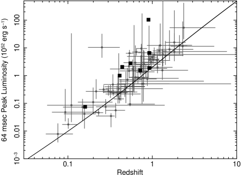
Figure 1.— The redshift distribution of SGRBs estimated by the $E_{p}$–luminosity correlation by (Tsutsui et al., 2013). The solid squares are known redshift samples, and the solid circles are ones of pseudo redshift. The solid line is the flux limit of $4\times 10^{-6}~{}{\rm erg~{}cm^{-2}s^{-1}}$

Figure 2.— The correlation between the $E_{p}$ values of this work (Band function) and the ones of Ghirlanda et al. (2009) (CPL function). The solid line is an equivalent line. Both results strongly correlate with each other, but our results are slightly smaller than the one of Ghirlanda et al. (2009) for almost all samples. This trend comes from the different model function of spectral analyses as Kaneko et al. (2006) pointed out.

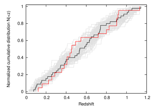
Figure 3.— The cumulative redshift distribution of SGRBs up to $z=1.14$. The black and the red solid lines are for 45 BATSE SGRBs in this paper and 22 known redshift samples observed by HETE-2 and Swift/BAT, respectively. The gray solid lines behind them show possible error regions estimated by 100 Monte Carlo simulations. We can see the good agreement of red, black and gray lines in the entire region. Kolmogorv-Smirnov test between black and red lines shows that the probability that the two curves arise from different distribution is 79.4 %, and the error region shown in gray lines covers the red line. This strongly suggests that the $E_{p}$–$L_{p}$ correlation for SGRB (Tsutsui et al., 2013) is a good distance indicator.

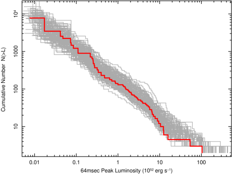
Figure 4.— The luminosity function of SGRBs estimated from data distribution of figure 1. The red solid line shows one of the best estimation, and 100 gray lines are possible error region estimated by the Monte Carlo simulations. We can approximately describe it as a simple power-law function with the index of $-1$, and no obvious break has been found.

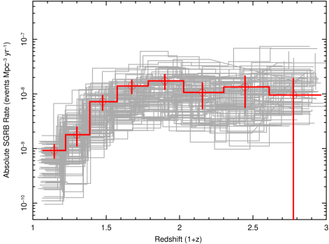
Figure 5.— Absolute formation rate of SGRBs estimated from data distribution of figure 1. Again the red line is the best estimation and 100 gray lines are ones from Monte Carlo simulations. The local event rate at $z=0$ is $\rho_{SGRB}(0)=6.3^{+3.1}_{-3.9}\times 10^{-10}~{}{\rm events~{}Mpc^{-3}yr^{-1}}$.

References

- Aasi et al. (2013) Aasi, J., Abadie, J., Abbott, B. P., et al. 2013, arXiv:1304.0670
- Abadie et al. (2010) Abadie, J., Abbott, B. P., Abbott, R., et al. 2010, Classical and Quantum Gravity, 27, 173001
- Amati et al. (2002) Amati, L., Frontera, F., Tavani, M, et al. 2002, A&A, 390, 81
- Amati (2006) Amati, L., 2006, MNRAS, 372, 233
- Band et al. (1993) Band, D.L., Matteson, J., Ford, L., et al. 1993, ApJ, 413, 281
- Berger (2013) Berger, E. 2013 arXiv:1311.2603
- Coward et al. (2012) Coward, D.M., Howell, E.J., Piran, T. et al. 2012, MNRAS, 425, 2668
- Dainotti, Petrosian, Singal et al. (2014) Dainotti, M. G., Petrosian, V., Singal, J., et al., 2014, ApJ, 774, 157
- Dietz (2011) Dietz, A., 2011, A&A, 529, A97
- Efron & Petrosian (1992) Efron, B. & Petrosian, V., 1992, ApJ, 399, 345
- Fong et al. (2012) Fong, W., Berger, Margutti, R. et al. 2012, ApJ, 756, 189
- Fong et al. (2013) Fong, W., Berger, E.,Chornock, R. et al. 2013, ApJ, 769, 56
- Fong et al. (2014) Fong, W., Berger, E.,Metzger, B.D. et al. 2014, ApJ, 780, 118
- Ghirlanda et al. (2004) Ghirlanda, G., Ghisellini, G., Lazzati, D., 2004, ApJ, 616, 331
- Ghirlanda et al. (2005a) Ghirlanda, G., Ghisellini, G., Firmani, C., 2005a, MNRAS, 361, L10
- Ghirlanda et al. (2005b) Ghirlanda, G. et al., 2005b, MNRAS, 360, L45
- Ghirlanda et al. (2009) Ghirlanda, G., Nava, L., Ghisellini, G., et al. 2009, A&A, 496, 585-595
- Guetta & Piran (2005) Guetta, D., & Piran, T., 2005, A&A, 435, 421
- Guetta & Piran (2006) Guetta, D., & Piran, T., 2006, A&A, 453, 823
- Harrison et al. (1999) Harrison, F. A., Bloom, J. S., Frail, D. A. et al. 1999, ApJ, 523, 121
- Kalogera et al. (2004a) Kalogera, V., Kim, C., Lorimer, D. R. et al. 2004, ApJ, 601, L179
- Kalogera et al. (2004b) Kalogera, V., Kim, C., Lorimer, D. R. et al. 2004, ApJ, 614, L137
- Kaneko et al. (2006) Kaneko, Y., Preece, R. D., Briggs, M. S., et al. 2006, ApJS, 166, 298
- Krimm et al. (2009) Krimm, H. A., et al. 2009, ApJ, 704, 1405
- Lloyd-Ronning, Petrosian & Mallozzi (2001) Lloyd-Ronning, N. M., Petrosian, V. & Mallozzi, R. S., 2001, ApJ, 534, 227
- Lynden-Bell (1971) Lynden-Bell, D., 1971, MNRAS, 155, 95
- Maloney & Petrosian (1999) Maloney, A. & Petrosian, V., 1999, ApJ, 518, 32
- Metzger & Berger (2012) Metzger, B. D., & Berger, E., 2012, ApJ, 746, 48
- Nakar, Gal-Yam & Fox (2006) Nakar, E., Gal-Yam, A., & Fox, D. B., 2006, ApJ, 650, 281
- Nicuesa Guelbenzu et al. (2011) Nicuesa Guelbenzu, A., Klose, S., Rossi, A. et al. 2011, A&A, 531, L6
- O’Shaughnessy & Kim (2010) O’Shaughnessy, R. & Kim, C. 2010, ApJ, 715, 230
- Petrillo, Dietz & Cavaglia (2013) Enrico Petrillo, C.; Dietz, A.; Cavaglia, M., 2013, ApJ, 767, 140
- Petrosian (1993) Petrosian, V., 1993, ApJ, 402, L33
- Rhoads (1999) Rhoads, J. E. 1999, ApJ, 525, 737
- Seto, Kawamura & Nakamura (2001) Seto, N., Kawamura, S., & Nakamura, T. 2001, Physical Review Letters, 87, 221103
- Soderberg et al. (2006) Soderberg, A. M., Berger, E., Kasliwal, M. et al. 2006, ApJ, 650, 261
- Tsutsui et al. (2013) Tsutsui, R., Yonetoku, D., Nakamura, T. et al. 2013, MNRAS, 431, p.1398
- Yonetoku et al. (2004) Yonetoku, D., Murakami, T., Nakamura, T. et al., 2004, ApJ, 609, 935
- Yonetoku et al. (2010) Yonetoku, D., Murakami, T., Tsutsui, R. et al., 2010, PASJ, 62, 1495