Imaging Redshift Estimates for Fermi BL Lacs

Abstract

We have obtained WIYN and SOAR $i^{\prime}$ images of BL Lacertae objects (BL Lacs) and used these to detect or constrain the flux of the host galaxy. Under common standard candle assumptions these data provide estimates of, or lower bounds on, the redshift. Our targets are a set of flat-spectrum radio counterparts of high flux Fermi Large Area Telescope (LAT) sources, with sensitive spectral observations showing them to be continuum-dominated BL Lacs. In this sample 5 of 11 BL Lacs yielded significant host detections, with standard candle redshifts $z=0.13-0.58$. Our estimates and lower bounds are generally in agreement with other redshifts estimates, although our $z=0.374$ estimate for J0543$-$5532 implies a significantly sub-luminous host.

1. Introduction

BL Lac objects are an important, extreme sub-class of AGN. The large numbers of BL Lacs being detected in the gamma-rays by the Fermi LAT (Ackermann et al, 2011) show that these blazars are a dominant contributor to the GeV sky. This flux-limited gamma-ray sample also provides a unique opportunity to probe the evolution of the BL Lac phenomenon over cosmic time (Ajello et al, 2014). BL Lac evolution is controversial, with various authors finding negative (e.g. Rector et al, 2000), positive (e.g. Marcha & Caccianiga, 2013) or negligible evolution (e.g. Caccianiga et al, 2002). Much of this uncertainty stems from the difficulty in determining redshifts; for many BL Lacs the high jet-associated continuum flux dominates emission from any broad-line region and results in very low equivalent width for galactic host absorption features. Despite intensive spectroscopic campaigns (Shaw et al, 2013b) this often precludes direct BL Lac redshift measurement, challenging their utility for population and evolution studies (Ajello et al, 2014). Thus alternate methods of estimating or constraining the source redshift can be quite valuable (Shaw et al, 2013a).

In this paper, we image Fermi BL Lacs to search for host flux in the wings of the nuclear point spread function (PSF). Our targets are drawn from the ‘2LAC’ (Ackermann et al, 2011) LAT blazars for which sensitive spectroscopy, reported in Shaw et al (2013b), shows them to be continuum-dominated BL Lacs at very high significance, but was not able to determine a redshift. Since hosts are increasingly difficult to detect at high redshift, we excluded BL Lacs whose spectra showed intervening absorbers requiring $z>0.7$ or excluded continuum flux from hosts at lower $z$; this left 226 targets. We observed objects from this list when conditions and gaps in other observing programs allowed.

It has been argued that BL Lac hosts are nearly uniform giant ellipticals with $M_{R}$ = $-$22.5 (Sbarufatti et al, 2005). Thus several authors have used such imaging to constrain the source redshift (e.g. Sbarufatti et al, 2005; Meisner & Romani, 2010; Nilsson et al, 2012). One can also search for the elliptical flux in high S/N spectra; when not detected this provides a lower limit on the redshift (e.g. Sbarufatti et al, 2006; Shaw et al, 2013b; Sandrinelli et al, 2013). Conversely, when direct spectroscopic redshifts measurements are in hand (or later become available), the flux measurements can be used to test the standard candle hypothesis and the evolution of the BL Lac hosts. Here, we follow the method described by Meisner & Romani (2010), although we use an updated host magnitude calibration derived from absorption lines features measured in a deep spectroscopic survey (Shaw et al, 2013a).

2. Observation and Data Reduction

Our typical BL Lac has a total magnitude of $i^{\prime}\sim 15-18$. We wish to model our individual image point spread function (PSF), following the wings to well below the sky brightness, and to test the PSF model against a number of stars with flux comparable to that of the BL Lac core. Thus we need moderate field imaging with good natural seeing. For this program we used the Mini-Mosaic (MiniMo) camera at the WIYN 3.6m telescope at Kitt Peak National Observatory and the SOAR Optical Imager (SOI) at the SOAR 4.2m telescope on Cerro Pachon. Individual exposures ($t_{exp}=180$ s$-600$ s) were adjusted to minimize the core saturation; the pointing was dithered between exposures. All data were taken using an SDSS i^′ filter.

2.1. MiniMo

Observations with MiniMo were made on the nights of September 26-27, 2011 and February 17-18, 2012. The mosaic image consists of two $2048\times 4096$ chips, with a plate scale of 0.141^′′/pixel, separated by a 7.8^′′ gap. This gives a field of 9.6 arcmin$\times$9.6 arcmin.

2.2. SOI

Observations with SOI were made on the nights of March 21-23, 2012. The SOI mosaic also has two $2048\times 4096$ chips, again split by a 7.12^′′ gap. Seeing was only moderate quality during the run, so we observed with 2x2 binning, for a plate scale of 0.153^′′/binned pixel and a 5.2 arcmin$\times$5.2 arcmin FoV. We targeted 5 dithered exposures for each object. We generally suffered significant core saturation for the brighter BL Lacs.

Table 1Observations and Fitted Component Amplitudes and Errors

Name	SIMBAD Name	Tel	Exp (s)	DIQ(′′)	$N_{PSF}$	Corea	Hosta	$\sigma_{stat}^{a}$	$\sigma_{sys}^{a}$
J0114+1325	GB6 J0114+1325	W	$3\times 300$	0.72	26	2160	144	5.47	43.8
J0115+2519	RX J0115.7+2519	W	$3\times 300$	0.79	21	1050	377	5.27	18.8
J0222+4302	3C 66A	W	$5\times 300$	0.68	36	13500	229	7.77	315.
J0316+0904	GB6 J0316+0904	W	$5\times 300$	0.63	27	1910	133	4.18	61.5
J0543$-$5532	1RSX 053810.0$-$390839	S	$5\times 300$	0.57	20	3410	638	6.82	108.
J0558$-$7459	PKS 0600-749	S	$5\times 180$	0.69	24	1260	-24	7.29	56.7
J0700$-$6610	PKS 0700-661	S	$4\times 300$	1.06	19	4950	81	6.70	147.
J0721+7120	S5 0716+71	W	$600+3\times 300$	1.34	19	39700	5430	16.0	812.
J1023$-$4336	RX J1023.9$-$4336	S	$5\times 300$	0.62	21	8610	120	10.3	106.
J1026$-$8543	PKS 1029$-$85	S	$1\times 300$	0.83	16	2150	10	6.21	88.6
J1110$-$1835	CRATES J1110$-$1835	S	$5\times 180$	0.61	9	372	9	3.84	20.0

Tabulated quantities: Name, Simbad Name, Telescope, exposure used, final combined image full width at half maximum, number of

PSF stars used, fit core (PSF) count rate, fit host count rate, statistical error on host rate, estimated systematic error on host rate.

^a counts/s.

2.3. Data Processing

All images were reduced using the IRAF mscred package for mosaic image data. Standard zero image bias subtraction and dome flats were applied and cosmic rays were cleaned using the IRAF xzap package. A few bad pixel/cosmic ray events were edited by hand. The $i^{\prime}$ fringing was quite modest, especially for the chip hosting the BL Lac target, so no fringe corrections were made.

After generation of a world coordinate system (WCS) for each frame using the USNO B-1 reference catalog, the dithered frames were stacked to a median combined frame. In general, the PSF varied relatively slowly during the observations. In a few cases, we rejected the worst sub-frames before the final image combination. The final exposures included in the image stack and the stacked image FWHM are listed in Table 1.

3. Image Modeling

Our goal is to measure the unresolved AGN core and surrounding resolved host galaxy, extracting reliable fluxes or flux upper limits for the latter. To this end we model cut-outs around each BL Lac. Typically we treated a $10^{\prime\prime}\times 10^{\prime\prime}$ region, although for 1 object we used a $22^{\prime\prime}\times 22^{\prime\prime}$ region to contain the bulk of the host counts, and for 2 other objects we were able to reduce the region size to $6^{\prime\prime}\times 6^{\prime\prime}$ while containing all the host flux.

3.1. Model Components

Since we are interested in the faint host excess in the wings of the AGN PSF, we need an accurate PSF for each final combined image frame. These PSFs were generated using the IRAF daophot package. Generally over 20 bright isolated stars were available to generate the PSF, although a few fields were more sparse. Saturated stars were not included in the PSF stack. For most cases our PSF model extends to 5^′′, where the host contribution drops well below the sky, however for 2 objects with the best PSF we used 3^′′ and for the target with the worst seeing we extended the PSF model to 11^′′. Since we needed much of the field to include sufficient bright stars, we used a quadratic variation across the image for the analytic PSF core. The accuracy of the PSF model was checked by generating a model (using the quadratic position-dependent PSF) for the precise positions of a set of check stars in each image. The residuals after subtraction were very small well out into the PSF wings, although as expected, poor subtraction was often present for near-saturated cores within 1 FWHM. The target PSF model was generated for the field position of the BL Lac.

Based on previous studies of BL Lac host galaxies (Scarpa et al, 2000; Urry et al, 2000), we assume that our hosts are well modeled by a de Vaucouleurs profile of Sersic index 4. In addition to the integrated model flux we have up to three shape parameters. For bright, well resolved hosts, we can fit the effective angular size $\theta_{e}$. If not fit, we fix this at $\theta_{e}=1.65^{\prime\prime}$, which corresponds to R${}_{e}=$10 kpc at a typical BL Lac $z=0.5$ for our standard approximate concordance cosmology ($\Omega_{m}=0.3$, $\Omega_{\Lambda}=0.7$, $H_{0}=70$km s^-1 Mpc^-1). Occasionally resolved hosts show significant ellipticity; we then fit this along with the position angle. Before fitting the model profile is convolved with the locally generated model PSF for the particular image.

3.2. Fitting Procedure

In all cases, we use the AGN core position (fit with IRAF DAOPHOT) determined at sub-pixel accuracy to generate the normalized templates for the PSF and PSF-convolved host models. The core and host position were not adjusted in the fit. Before fitting we masked saturated pixels (counts $>35,000$DN) which typically excluded $\sim 1$FWHM around the PSF core and for the brightest sources, a modest number of pixels in a bleed trail. We also had the option of masking pixels associated with neighboring sources (companion galaxies and field stars). This was done for 3 sources.

We fit the masked cut-out images with $\chi^{2}$ minimization of the residuals to the model counts in each image pixel, using a Nelder-Mead downhill simplex algorithm (scipy, 2004). Host shape parameters are determined hierarchically. If a statistically significant amplitude is fit ($>3\sigma_{\rm stat}$) using the default spherical host with fixed $\theta_{e}$, we re-fit allowing $\theta_{e}$ to vary. If $\theta_{e}$ is measured with high statistical significance, we re-fit including the ellipticity and position angle of the host. In this data set only three sources had a well measured effective radius and only one had significant ellipticity. The routine returns best fit values for the PSF, host and constant background counts, up to three additional host shape parameters, and statistical errors on each fit quantity.

3.3. Systematic Errors

Inevitably, due to peculiarities of the actual image and imperfections in the model PSF, we expect systematic errors to dominate the simple fit statistical errors. To estimate the systematic errors on the host fitting, we selected $\sim$10 bright stars in each image, generated the local PSF and fit for combined PSF, de Vaucouleurs (fixed $\theta_{e}$) ‘host’ and uniform background counts. Ideally these would be not be drawn from the PSF stars, but we did not always have enough bright stars to avoid overlap. The fit ‘host’ counts give an estimate of the systematic host errors. Figure 1 shows the distribution of fit ‘host’ counts, as a fraction of the stellar (PSF) counts. The mean of zero suggests good model PSFs with no overall bias.

Figure 1.— Distribution of fit ’host’ counts to PSF counts for fits to isolated stars. The symmetric distribution centered on zero shows that, across all fields, there is little overall systematic bias in the PSF model.

In figure 2 we show the absolute value of the individual fit ‘host’ counts plotted as a function of PSF counts. If the errors were purely statistical we would expect a square-root scaling, instead the upper envelope of the distribution is approximately linear (solid line), suggesting that for bright PSFs the dominant errors are indeed systematic. The figure also show the statistical fit errors for the individual BL Lacs, with the expected $\sim$square root trend (dashed line). Note that the distribution of systematic ‘host’ amplitudes fit to stars lies above this trend, with statistical errors significant when the PSF contains less than $\sim 10^{4}$ counts and systematics increasingly dominating for brighter stars.

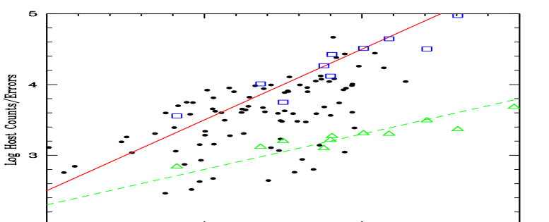
Figure 2.— Here black points show the distribution of the fit ‘host’ counts fit for isolated stars, plotted as a function of the PSF counts. Open triangles show the statistical errors to the BL Lac host fits, while open squares show our estimate of the systematic host error for each BL Lac field (see text).

Since the systematic errors grow linearly with PSF flux, for each BL Lac field we normalize the stellar ‘host’ fits to the PSF flux, take the RMS of this distribution as $f_{rms}$ and compute $\sigma_{sys}=f_{rms}\times N_{AGN}$, where $N_{AGN}$ is the fit core counts, to be our estimate of the systematic error in our host count estimate. These errors (Figure 2) lie $\sim 5-10\times$ above the $\sigma_{\rm stat}$ fitting errors for the corresponding field. We believe that this estimate is conservative, as the resulting errors lie at the upper envelope of the individual stellar ‘host’ errors.

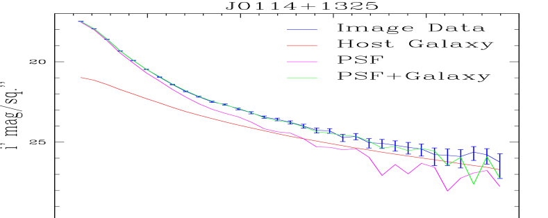
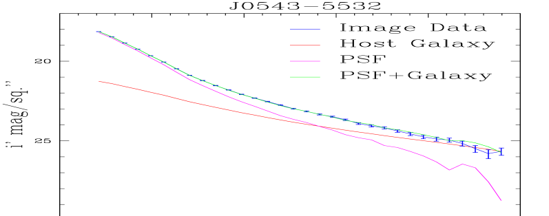
Figure 3.— Two objects with significant host detections. Left: J0114+1325 (WIYN), Right: J0543-5532 (SOAR). The inferred redshifts are $z\approx 0.58$ and $z\approx 0.37$, respectively. The lines show the profile of the best-fit model components, converted to magnitudes/arcsec². For both the host counts dominate the PSF beyond $\sim 2.7^{\prime\prime}$.

3.4. Fitting Results

The final fit component counts and the statistical and systematic errors are listed in Table 1. We also list the calibrated core magnitudes and host flux ratios in Table 2, where we convert $i^{\prime}$ image counts to instrumental band flux using calibration stars from the SDSS.

To claim a significant host detection, we require that the fit counts exceed $\sqrt{3\sigma_{stat}^{2}+\sigma_{sys}^{2}}$. Four of our BL Lac hosts are detected at very high significance. Two are seen with somewhat lower confidence, with J0316+0904 having $\sim 2.2\sigma_{sys}$ significance and J1023$-$4336 appearing at $\sim 1.1\sigma_{sys}$ (although both are of high statistical significance). Visual inspection of the images and the azimuthally average radial profile plots (below) confirm that the former is a very likely detection, but the latter, while a plausible detection, may be more safely treated as an upper limit. When we have no significant host detection, we infer host flux counts to be $<\sqrt{3\sigma_{stat}^{2}+\sigma_{sys}^{2}}$.

Only three sources have significant $R_{e}$ measurements listed. These well measured sizes are all consistent with the standard 10 kpc assumption. J0115+2519 was the only source with a statistically significant ellipticity $e=0.160\pm.043$; this is at major axis position angle $-16.1\pm 3.5^{\circ}$, measured North through East.

It is convenient to display these fits as azimuthally averaged profiles of the surface brightness. In figure 3 we show two sources with well-detected hosts. Figure 4 shows two sources with radial profiles well matched to the PSF, resulting in host upper limits. Error flags on the data curves show the $1\sigma$ fluctuations assuming Poisson statistics.

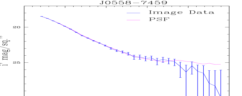
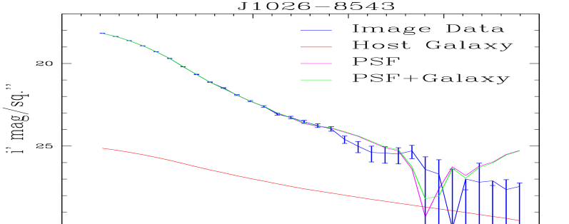
Figure 4.— Two objects providing host upper limits. Left: J0558$-$7459 whose fit amplitude is in fact negative, so no host model is shown; the inferred limit is $z>0.66$. Right: J1026$-$8543 has an insignificant host detection. We infer $z>0.62$

4. Redshift Estimates and Conclusions

A primary goal of this exercise is to use the host fluxes to constrain the source redshift, adopting the standard candle hypothesis. To this end we use the Hubble diagram curve computed in Meisner & Romani (2010). This curve follows an elliptical host formed at $z=2$ and evolving according to the Fioc & Rocca-Volmerange (1997) models to the observed $z$ in our standard cosmology, computing the observed flux by folding through the $i^{\prime}$ filter. However, a recent spectral survey of Fermi BL Lacs (Shaw et al, 2013a) finds that the host luminosity of these $\gamma$-ray sources is 0.4 magnitudes fainter than the $M_{R}$ = -22.9 $\pm$ 0.5 reported by Sbarufatti et al (2005). We thus amend the Hubble diagram by normalizing the evolving models to this decreased luminosity at $z=0$.

Figure 5.— $i^{\prime}$ Hubble diagram for gamma-ray BL Lac hosts, after Meisner & Romani (2010), but normalized to a standard candle magnitude $M_{R}=-22.5$.

Using this curve we translate the host magnitude values and upper and lower statistical and systematic errors to redshift estimates and error ranges. These are reported in Table 2. When only an upper limit on the flux is available, this translated to a redshift lower limit. The redshift estimates for detected hosts varied from 0.13 to 0.58, with lower limits $0.42-0.93$. We consider these limits conservative, in the sense that we use the revised (less luminous) standard candle calibration above. However, insofar as some BL Lacs undoubtedly have substantially sub-luminous hosts, individual sources may indeed appear at lower $z$.

Table 2Fitting Results: Calibrated Magnitudes, Sizes and Redshifts

Name	SEDa	i′nucl	i′Host	$f_{host}/f_{nucl}$	Re (kpc)	$z_{im}$	$z_{sp}$
J0114+1325	H	17.21	20.15${}_{-0.037-0.29}^{+0.038+0.41}$	0.07	8.32$\pm$0.14	0.583${}_{-0.006-0.052}^{+0.007+0.064}$	$0.61-1.63$
J0115+2519	H	17.68	18.80${}_{-0.015-0.05}^{+0.015+0.05}$	0.36	12.53$\pm$0.55	0.358${}_{-0.001-0.006}^{+0.001+0.007}$	$0.37-1.63(>0.268)$
J0222+4302	I	15.13	$>$19.21	$<$0.02	-	$>$0.42	$0.12-1.67$
J0316+0904	H	16.01	18.91${}_{-0.033-0.412}^{+0.035+0.672}$	0.07	-	0.372${}_{-0.004-0.076}^{+0.005+0.103}$	$0.12-1.66$
J0543$-$5532	H	17.10	18.92${}_{-0.012-0.17}^{+0.012+0.20}$	0.19	-	0.374${}_{-0.002-0.023}^{+0.003+0.027}$	$0.27-2.57$[=0.273]
J0558$-$7459	-	17.23	$>$20.52	$<$0.05	-	$>$0.66	$0.29-2.20(>0.475)$
J0700$-$6610	I	16.28	$>$20.08	$<$0.03	-	$>$0.57	$0.39-1.92$
J0721+7120	I	14.01	16.17${}_{-0.0024-0.193}^{+0.0038+0.237}$	0.14	9.54$\pm$0.32	0.127${}_{-0.001-0.073}^{+0.002+0.092}$	$0.14-2.61$
J1023$-$4336	H	15.26	19.90${}_{-0.090-0.689}^{+0.090+2.36}$	0.03	-	b0.534${}_{-0.014-0.115}^{+0.019+0.482}$	$0.34-2.24$
J1026$-$8543	L	16.88	$>$20.31	$<$0.04	-	$>$0.62	$0.32-2.30$
J1110$-$1835	L	18.69	$>$21.70	$<$0.06	-	$>$0.93	$0.51-2.23$

Tabulated quantities: Name, SED class, Core magnitude, host magnitude and errors or limit, host radius,

inferred redshift or limit, spectroscopic constraints on redshift

^a SED class from Ackermann et al (2011), based on the synchrotron peak frequency.

^b Good statistical, but marginal $\sim 1\sigma$ systematic significance. Corresponding lower limit is $z>0.42$

Shaw et al (2013a) analyzed high S/N spectra of a large number of Fermi BL Lacs. In a method parallel to the present imaging host search, they detected or placed limits on the BL Lac host by measuring the flux of a spectral component from a standard candle elliptical. After appropriate k-correction and slit-loss corrections, these measurements provided host redshift estimates or lower bounds. In addition, sometimes intervening metal line absorption systems were detected. These provide firm, model-independent lower bounds on the host redshift. These spectroscopically allowed ranges and lower bounds are listed in the last column of Table 2; we give here the ranges derived for a standard candle magnitude $M_{R}$ = -22.5, for consistency with our imaging results.

Since in this program we targeted BL Lacs without known redshift, none of our sources has a spectroscopic $z$ in Shaw et al (2013a). For the five sources with host detection, two (J0316+0904 and J0543$-$5532) have imaging redshift estimates consistent with the spectra-derived bounds in that paper; the low significance detection of J1023$-$4336 is also consistent. Three (J0114+1325, J0115+2519, and J0721+7120) lie at slightly lower $z$ than the spectral lower bound, but are within 3$\sigma$, and J0115+2519 is fully consistent with the strict lower limit provided by an intervening absorber. However, since completing this study Pita et al (2013) have published new high quality VLT/X-shooter spectra of a number of blazars, including J0543$-$5532, measured here. For this source, they infer $z=0.237$ based on a weak Ca II H/K doublet and a Na I absorption line. This redshift, near the lower bound of Shaw et al (2013a) is well below our imaging estimate, implying a host that is substantially fainter than our standard candle assumption. At this $z$ our measured host flux implies an absolute magnitude $M_{R}=-21.67^{+0.01+0.20}_{-0.01-0.17}$, $0.8$mag ($1.7\sigma$) away from our assumed standard candle luminosity. The host absolute magnitude is consistent with, but more accurate than, the spectroscopically estimated value in Pita et al (2013).

In six cases we derive lower bounds on the redshift; J1023$-$4336 may be interpreted as a lower bound of $z>0.42$. These limits are always more constraining than those extracted from the spectroscopic study. For J0558$-$7459 our new bound is also stronger than that obtained from the intervening absorption line system. Thus these bounds may be useful in BL Lac population studies (e.g. Ajello et al, 2014).

With median $f_{host}/f_{nucl}=0.07$ our sources are very strongly dominated by the non-thermal nuclear core flux. This is in contrast to the HST study of Scarpa et al (2000), where of 69 BL Lacs with resolved hosts, 37 had $f_{host}/f_{nucl}>1$. Our large core dominance is similar to that found in Meisner & Romani (2010) and, as noted there, it may be attributed to the fact that these are gamma-ray selected BL Lacs and thus should have high alignment between the jet axis and the Earth line-of-sight, increasing the core dominance. In addition, these sources were drawn from the BL Lacs lacking redshifts even after extensive spectroscopy with 8 m-class facilities (Shaw et al, 2013a, b). Since sources with brighter hosts allow easier absorption line redshift measurements, the remainder (including the sources studied here) should have an especially high core dominance.

In previous studies (Scarpa et al, 2000; Urry et al, 2000; Meisner & Romani, 2010) the BL Lacs were seen to have an excess of faint galactic companions, indicating that they were located in cluster environments and that they may have recent interaction activity. In general, the relatively poor seeing and modest image depth achieved during this project prevented us from identifying very faint companions. For 2 objects, we did find bright companion galaxies nearby. J0114+1325 had two companions within a 3^′′ ($\sim 20$ kpc) radius. These companions were close enough that they overlap significantly with the BL Lac host wings, making accurate flux measurement difficult; we found their i^′ magnitudes to be roughly 20.5 and 20.8. J0222+4302 had 4 surrounding bright companions located 11$-12^{\prime\prime}$ ($\sim 70$ kpc) from the core, with i^′ magnitudes of 18.9, 19.3, 19.5, and 20.9.

We have detected hosts in the images of 5/11 BL Lacs, plus one marginal detection. Assuming a standard candle host luminosity these provided redshift estimates $z=0.127-0.583$ ($z_{med}$ = 0.37). The minimum redshifts for the remainder are also larger than available spectroscopic lower limits and so are useful, as well. Perhaps unsurprisingly, our host detections were for four HBLs (high spectral peak energy, relatively low luminosity) sources and one intermediate peak source. The other intermediate peak sources and the two LBLs (low peak, higher power) sources in our sample yielded only lower limits on $z$; these include the highest limit, $z>0.93$ in this sample.

When no other redshift estimate is available, these imaging-derived values can be useful for statistical purposes, e.g. in population studies. However, as emphasized by the spectroscopic $z$ recently derived for J0543$-$5532, the standard candle hypothesis is only statistically useful, at best, and should be subject to further study. Indeed Pita et al (2013) estimate that two of their BL Lac hosts have $M_{R}<-24$, even further from the expected standard candle value. Our host flux measurements thus remain useful whenever an independent redshift is derived. The prospects for further spectroscopic redshifts of our imaged hosts are, in fact, good; these are excellent targets for spatially resolved spectroscopy, especially with Integral Field Unit (IFU) feeds, which can isolate host spectral features from the wings of the BL Lac.

References

- Ackermann et al (2011) Ackermann, M. et al. 2011, ApJ, 743, 171
- Ajello et al (2014) Ajello, M. et al. 2014, ApJ, 780, 73
- Caccianiga et al (2002) Caccianiga, A. et al.2002, ApJ, 556, 181
- Fioc & Rocca-Volmerange (1997) Fioc, M. & Rocca-Volmerange, B. 1997, AA, 326, 950
- Marcha & Caccianiga (2013) Marcha, M.J.M. & Caccianiga, A. 2013, MNRAS, 430, 246
- Meisner & Romani (2010) Meisner, A.M. & Romani, R.W. 2010, ApJ, 712, 14
- Nilsson et al (2012) Nilsson, K. et al. 2012, AA, 457, A1
- Pita et al (2013) Pita, S. et al. 2013, AA, in press, arXiv/1311.3809
- Rector et al (2000) Rector, T.A. et al. 2000, AJ, 120, 1626
- scipy (2004) Scipy, docs.scipy.org/scipy.optimize.fmin.html
- Sandrinelli et al (2013) Sandrinelli, A. et al. 2013, AJ, 146, 163
- Sbarufatti et al (2005) Sbarufatti, B. et al. 2005, ApJ, 635, 173
- Sbarufatti et al (2006) Sbarufatti, B. et al. 2006, AA, 457, 35
- Scarpa et al (2000) Scarpa, R. et al. 2000, ApJ, 532, 740
- Shaw et al (2009) Shaw, M.S., et al. 2009, ApJ, 704, 477
- Shaw et al (2013a) Shaw, M.S., et al. 2013, ApJ, 764, 135
- Shaw et al (2013b) Shaw, M.S., et al. 2013, AJ, 146, 127
- Urry et al (2000) Urry, C.M. et al. 2000, ApJ, 532, 816