Crossovers in the dynamics of supercooled liquids probed by an amorphous wall

Abstract

We study the relaxation dynamics of a binary Lennard-Jones liquid in the presence of an amorphous wall generated from equilibrium particle configurations. In qualitative agreement with the results presented in Nature Phys. 8, 164 (2012) for a liquid of harmonic spheres, we find that our binary mixture shows a saturation of the dynamical length scale close to the mode-coupling temperature $T_{c}$. Furthermore we show that, due to the broken symmetry imposed by the wall, signatures of an additional change in dynamics become apparent at a temperature well above $T_{c}$. We provide evidence that this modification in the relaxation dynamics occurs at a recently proposed dynamical crossover temperature $T_{s}>T_{c}$, which is related to the breakdown of the Stokes-Einstein relation. We find that this dynamical crossover at $T_{s}$ is also observed for the harmonic spheres as well as a WCA liquid, showing that it may be a general feature of glass-forming systems.

I Introduction

There has been a great surge in studies which seek to investigate length scales in supercooled liquids through simulation in the presence of quenched amorphous order Biroli et al. (2008); Kim et al. (2009); Kob et al. (2012a); Jack and Berthier (2012); Karmakar et al. (2012); Berthier and Kob (2012); Charbonneau et al. (2012); Hocky et al. (2012); Charbonneau and Tarjus (2013); Kob and Berthier (2013); Jack and Fullerton (2013). This recent interest has been spurred on by the successful computational realization of thought experiments predicting growing static length scales on increased supercooling, as well as the ever-growing availability of CPU time which makes such studies feasible Bouchaud and Biroli (2004); Biroli et al. (2008); Cammarota et al. (2011); Berthier and Kob (2012); Charbonneau et al. (2012); Hocky et al. (2012); Charbonneau and Tarjus (2013); Kob and Berthier (2013); Karmakar et al. (2012); Jack and Fullerton (2013).

Yet, studies seeking to understand growing dynamical length scales by employing simulations with frozen particles go back even earlier Scheidler et al. (2002); Kim (2003). The authors of Ref. Scheidler et al., 2002, in particular, studied the Kob-Andersen binary Lennard-Jones system (KA) in the presence of a rough wall created by fixing the positions of a slab of particles from a bulk equilibrium configuration. They found that the dynamics near the rough wall slowed down substantially and the analysis of the profiles of relaxation times near the wall provided a length scale which grew with decreasing temperature. A recent study revisited these ideas in a supercooled harmonic sphere system (HARM) for larger sample sizes and down to very low temperatures, below the mode-coupling temperature $T_{c}$ Kob et al. (2012a). This study revealed a dynamical length scale that first increased as $T$ approached $T_{c}$ from above, and then surprisingly decreased for $T<T_{c}$ Kob et al. (2012a). This behavior was attributed to a change in the dynamics below $T_{c}$ where collective particle rearrangements become predominant Kob et al. (2012a, b); Kob and Coslovich (2014). Such a change is naturally understood in the framework of the random first order transition (RFOT) theory Stevenson et al. (2006); Berthier and Biroli (2011), where a crossover between non-activated correlated relaxation to thermally activated cooperative dynamics is expected to take place.

It should be noted that the dynamical length scale defined in Ref. Kob et al., 2012a need not correspond to that extracted from study of the bulk four-point correlation function $S_{4}(k,t)$, but simply defines an independent dynamic correlation length scale associated with the spatial extent of the perturbation of dynamic relaxation near an amorphous wall. Although there is a formal connection between bulk correlations and dynamic response to an infinitesimal field in the linear response regime Berthier et al. (2007); Kim et al. (2013), the connection between these different approaches to measure dynamic correlation lengthscales in systems with glassy dynamics will not be addressed in this work, but is a worthy topic for future research.

Since at present the non-monotonic $T-$dependence of the dynamical length scale probed by an amorphous wall has been observed only in one model glass-former, it is important to investigate whether this phenomenon is general or not. In order to address this question we have performed a similar analysis in the widely studied KA system (the same model used in Ref. Scheidler et al., 2002). When taken together, the results of previous studies in Refs. Berthier et al., 2012, 2007; Flenner and Szamel, 2013 may be interpreted as suggesting that a crossover in the relaxation dynamics across the mode-coupling temperature exists but is weaker for the KA than the HARM system. Therefore we anticipate that if the non-monotonic evolution of dynamic profiles near an amorphous wall results from this crossover, then this effect should be less pronounced in the KA model. In the present work, we seek to assess this possibility and to better understand which features of supercooled liquids near an amorphous wall are generic. Given our findings in the KA system, we then extend our study to two other supercooled liquids. Furthermore we demonstrate that indications of an additional crossover at a temperature higher than $T_{c}$ may be uncovered by the investigation of dynamics close to an amorphous wall, therefore showing that there are in fact two crossover temperatures at which the dynamics is changing.

This paper is organized as follows. In Sec. II we discuss the models to be studied, as well as the details of the various calculations we will employ. In Sec. III we present the results of our analyses and comparison with the previous results of Ref. Kob et al., 2012a. In Sec. IV we present results comparing the dynamics in directions perpendicular and parallel to the wall, which reveal further information related to the dynamics of supercooled liquids. Finally, in Sec. V we conclude and discuss the impact of our results in the broader context of recent work on supercooled liquids.

II Models and Methods

In this paper, we present data for three model systems. Our primary system of interest is the Kob-Andersen Lennard-Jones model (KA), an 80:20 binary mixture of particles at density $\rho=1.2$ with very well characterized structural and dynamical properties Kob and Andersen (1995); Kob (1999). All quantities are reported in standard reduced units. In this model, we find the onset of slow dynamics occurs near $T_{o}\approx 1.0$, and the mode-coupling crossover has been previously reported as $T_{c}\approx 0.435$ Berthier and Tarjus (2010). We have fully equilibrated this model for the system size $N=1900$ particles in a cubic box for the temperatures $T=0.9$, 0.8, 0.7, 0.65, 0.625, 0.6, 0.575, 0.56, 0.55, 0.5, 0.48, 0.45, 0.435, and 0.432. Simulations were done with $NVT$ dynamics for $100\tau_{\alpha}^{\rm bulk}$ at each temperature using the LAMMPS package Plimpton (1995); $\tau_{\alpha}^{\rm bulk}$ was determined by calculating the self-intermediate scattering function, $F_{s}(k,t)=\frac{1}{N}\sum_{j=1}^{N}e^{i\mathbf{k}\cdot(\mathbf{x}_{j}(t)-\mathbf{x}_{j}(0))}$, and defining $F_{s}(k=7.25,t\equiv\tau_{\alpha}^{\rm bulk})=1/e$. Each equilibrated configuration was replicated three times along the $z-$axis to make a rectangular box of dimensions approximately $11.655\times 11.655\times 34.966$. The rectangular boxes were again simulated for $100\tau_{\alpha}^{\rm bulk}$ to remove the periodicity introduced by replicating the system. Each configuration was then tested for equilibration by calculating $F_{s}(k,t)$ for the first and second half of yet another $100\tau_{\alpha}^{\rm bulk}$ length trajectory. Only configurations whose dynamics showed no signs of aging (i.e. identical scattering functions for both halves of the trajectory) were used for subsequent steps.

To study these configurations with an amorphous wall, simulations were run where the positions of particles within a slab of width $W=3$ were held fixed. Since we simulate the KA system with a standard cutoff of the potential at $r_{\rm cut}=2.5$, this slab is effectively of infinite thickness as no particle on one side can interact directly or indirectly with those on the other side. This allows to determine the $z-$dependence of the static and dynamic properties of the system for distances up to $z_{max}=(34.966-3)/2\approx 15.98$. At each temperature, we ran molecular dynamics simulations of length $500$-$1000\tau_{\alpha}^{\rm bulk}$ for $30-45$ independent wall realizations to ensure both thermalization of a single realization, and a proper disorder average over the quenched disorder imposed by the frozen wall.

In addition to the KA system, we performed a similar set of studies for two other models. The first is the Weeks-Chandler-Andersen (WCA) version of the KA system Weeks et al. (1971), for which we performed simulations down to $T=0.325$ (the mode-coupling temperature is $T_{c}\approx 0.28$ Berthier and Tarjus (2010), and $T_{o}\approx 0.7$). For this model, identical box sizes were used as for the KA. The third model we study is the harmonic sphere system (HARM) of Ref. Kob et al., 2012a, which had been previously discussed O’Hern et al. (2002); Berthier and Witten (2009) ($T_{c}\approx 5.2$ Kob et al. (2012a), $T_{o}\approx 12$). As in Ref. Kob et al., 2012a, we use $N=4320$, however here we prepare the system analogously to the KA system, first equilibrating a sample containing 1440 particles, then replicating it to construct a box with dimensions approximately $12.873\times 12.873\times 38.620$. In this case, we used a wave vector $k=6.28$ to define the relaxation time of the system and other subsequent quantities, and a wall thickness of $W=2$, due to the very short ranged potential in this model. For the HARM and WCA models we ran simulations with $20-30$ independent wall realizations. For the WCA system we found, by looking at aging behavior in $F_{s}(k,t)$, that some trajectories crystallized after times on the order of several hundred bulk $\tau_{\alpha}$ at $T=0.35$ in the presence of the wall. The tendency to crystallize was more pronounced at $T=0.325$. Crystallization was evident from visual inspection as well as from a drop in the potential energy of samples which crystallized. These trajectories were excluded from our data, and hence our statistical confidence at these temperatures is reduced and a detailed analysis of temperatures close to the mode-coupling crossover was not possible.

For each model and for each trajectory, we have calculated the overlap, $q_{c}(z,t)$, and self-overlap, $q_{s}(z,t)$, as a function of time and distance ($z$) from the face of the wall. These quantities, which contain similar information as the coherent and incoherent intermediate scattering functions, are calculated by tiling the system outside of the wall into small boxes of side-length $l$ small enough such that they have occupation numbers (defined by the number of particle centers in a cell) $n_{j}\in\{0,1\}$. In a previous work it was determined that $l\approx 0.37$ was a good size to enforce this condition in the KA and WCA systems without making $l$ so small as to result in poor statistics Hocky et al. (2012). In the present study we choose $l=0.37597$ which tiles each short dimension of the samples into $\tilde{N}=31$ boxes, but we have checked that changing this parameter does not have any effect on the resulting physics. Similarly, we choose $l\approx 0.45$ for the HARM, and tested that this gives the same results as $l\approx 0.55$, the value used in Ref. Kob et al., 2012a (at that size, $n_{j}>1$ occasionally). We define, at each distance $z$ from the wall,

$$q_{c}(z,t)=\left\langle\frac{1}{\tilde{N}^{2}}\sum_{j=1}^{\tilde{N}^{2}}\frac{n_{j}(t^{\prime}+t)n_{j}(t^{\prime})}{\rho l^{3}}\right\rangle,$$ (1)

and

$$q_{s}(z,t)=\left\langle\frac{1}{\tilde{N}^{2}}\sum_{j=1}^{\tilde{N}^{2}}\frac{p_{j}(t)}{\rho l^{3}}\right\rangle,$$ (2)

where $p_{j}(t)$ is a function which is 1 if box $j$ is occupied by a particle at a reference time $t^{\prime}$ and later by the same particle at $t^{\prime}+t$. In a bulk system with no wall, $n_{j}(t)$ and $n_{j}(0)$ fully decorrelate as $t\to\infty$, so the correlation function $q_{c}(z,t)$ tends to the random value $q_{r}\equiv\rho l^{3}$. Hence we define $\tilde{q}_{c}(z,t)\equiv q_{c}(z,t)-q_{r}$ so that this function decays to zero in the bulk case. With the presence of the wall, this function will decay to a finite value termed $\tilde{q}_{c}(z,\infty)\geq 0$, which quantifies the strength of the static correlations imposed by the presence of the wall. We define the relaxation time of the self-overlap $\tau_{s}(z)$ by $q_{s}(z,\tau_{s}(z))=0.2$ .

We have also investigated a second measure of density relaxation, the self-intermediate scattering of particles found at distance $z$ from the wall,

$$F_{s}(\mathbf{k},z,t)=\left\langle\frac{1}{N(z)}\sum_{j=1}^{N(z)}e^{i\mathbf{k}\cdot(\mathbf{x}_{j}(t)-\mathbf{x}_{j}(0))}\right\rangle,$$ (3)

where this sum extends over the particles which start in a slab of width 1.0 at distance $z$ from the wall, but need not necessarily end in that slab. We then define scattering functions for relaxation parallel and perpendicular to the wall by using wave vectors which are aligned with the unit vectors $\hat{\mathbf{x}}$ and $\hat{\mathbf{z}}$ respectively. Thus, we define $F_{s}^{||}(z,t)\equiv F_{s}(\mathbf{k}=7.25\hat{\mathbf{x}},z,t)$ and $F_{s}^{\perp}(z,t)\equiv F_{s}(\mathbf{k}=7.25\hat{\mathbf{z}},z,t)$, and define $\tau^{||}$ and $\tau^{\perp}$ when the associated correlation functions decay to a value of $1/e$.

III Overlap relaxation times

III.1 Saturating dynamic length scale

The first question we wish to address is whether the non-monotonic growth of the dynamical length scale seen in Ref. Kob et al., 2012a is also found in models other than the HARM system. For this purpose we measure dynamical relaxation profiles by calculating $\tau_{s}(z)$ and $\tau_{c}(z)$ at a series of temperatures in the KA system. As discussed in Ref. Kob et al., 2012a, dynamical properties calculated from the self and collective overlaps give very similar physical results. However, as $q_{c}(z,t)$ decays to a plateau while $q_{s}(z,t)$ always decays to zero, it is easier to measure $\tau_{s}(z)$ with confidence as there is no need to include the long time limit of this correlation function as an additional fitting parameter. We therefore concentrate on properties derived from the self-overlap $q_{s}(z,t)$.

Before discussing these properties we note that, just as in the HARM system, the static overlap $\tilde{q}_{c}(z,\infty)$ decays exponentially with the distance $z$ at all temperatures in the KA system, and that the static length extracted by fitting this decay grows by only a small fraction of its value at high temperatures over the considered temperature range. These properties are discussed in Appendix A.

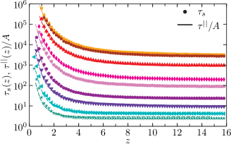
Figure 1: (Color online) Relaxation times in the KA system from self-overlap ($\tau_{s}$, points) and parallel self-intermediate scattering function ($\tau^{||}$, lines) versus the distance $z$ from the wall, shown for all studied temperatures. Error bars as determined from a bootstrap analysis Efron and Tibshirani (1993) are much smaller than the points shown. The second set of relaxation times is rescaled on the first one using a temperature independent rescaling constant $A=0.7$ obtained from $A=\tau^{||}(z=15,T=0.435)/\tau_{s}(z=15,T=0.435)$. From top to bottom: $T=0.432,$ 0.435, 0.45, 0.48, 0.5, 0.55, 0.6, 0.7, and 0.8.

The relaxation times $\tau_{s}(z)$ for different temperatures are shown in Fig. 1. As expected from previous studies, the dynamics slow dramatically near the wall, and relaxation times at a given distance increase with decreasing temperature Scheidler et al. (2002); Kob et al. (2012a). At large $z$ each curve tends to plateau before $z$ reaches a value corresponding to half of the box length. For comparison, we show that the relaxation times $\tau^{||}$ scale directly on top of the data from the self-overlap. demonstrating that the relaxation of the self-overlap is mostly dominated by relaxation in the parallel direction to the wall. This is reasonable since the dynamics in the direction perpendicular to the wall is significantly slower (see Sec. IV below), so that the self-overlap has already decayed by the time perpendicular motion sets in.

Based on earlier results for the KA model and results in the HARM system, we make the ansatz that the logarithm of the relaxation times in the presence of the wall decays exponentially to a plateau Scheidler et al. (2002); Kob et al. (2012a),

$$\ln(\tau_{s}(z))=B\exp\left(-z/\xi^{\rm exp}_{\rm dyn}\right)+\ln(\tau_{s}^{b}),$$ (4)

where $\tau_{s}^{b}$ is the bulk relaxation time, i.e. the relaxation time computed in the same manner but without the presence of the wall.

To extract the temperature dependence of the lengths in Fig. 1 we follow the recipe of Ref. Kob et al., 2012a. At each temperature we divide the data by $\tau_{s}^{b}(T)$ (these data can be found in Appendix B). We then fit the decay of $\ln(\tau_{s}(z)/\tau_{s}^{b})$ to Eq. (4) and extract the length scale $\xi^{\rm exp}_{\rm dyn}$ and the prefactor $B$. The results of this procedure can be seen in Fig. 2.

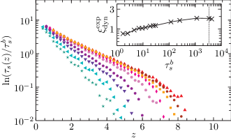
Figure 2: (Color online) Self-overlap relaxation times in the KA system at a distance $z$ from the wall are divided by the bulk relaxation for the given temperature. The temperatures and symbols shown are the same as in Fig. 1. By fitting these curves to Eq. (4), a dynamical length scale $\xi_{\rm dyn}^{\rm exp}$ is extracted, as shown in the inset for all temperatures listed in Sec. II. This length scale grows with decreasing temperature but saturates at a temperature above $T_{c}$, where $\tau_{s}^{b}\approx 3\times 10^{3}$, indicated by a vertical dotted line.

The inset of Fig. 2 shows the growth of the obtained dynamical length scale $\xi^{\rm exp}_{\rm dyn}$ and we recognize that $\xi^{\rm exp}_{\rm dyn}$ saturates for $T>T_{c}$. That this saturation is not just an artifact of the fitting procedure can be easily recognized from the data shown in the main panel of Fig. 2 which, for low temperatures, collapses almost perfectly onto a single master curve which implies that $\xi^{\rm exp}_{\rm dyn}$ depends only weakly on $T$. From this saturation we can conclude that our observed $T-$dependence of $\xi^{\rm exp}_{\rm dyn}$ is compatible with the results obtained for the HARM system Kob et al. (2012a), even if for the KA system there is no strong evidence for a non-monotonic behavior in $\xi^{\rm exp}_{\rm dyn}$ (although the length does appear to decrease very slightly). The absence of such a non-monotonic $T-$dependence in the KA system does not preclude the possibility of a change in behavior of $\xi_{\rm dyn}^{\rm exp}$ at lower temperatures. Indeed, it is expected that at temperatures below $T_{c}$, $\xi_{\rm dyn}^{\rm exp}$ will increase again at a temperature that is system dependent, and this behavior could supersede the non-monotonicity observed in the length scale of the HARM system Kob et al. (2012b).

That the $T-$dependence of $\xi^{\rm exp}_{\rm dyn}$ is less pronounced for the KA model than the HARM is also consistent with the results from Ref. Berthier et al., 2012 in which the relaxation dynamics of both KA and HARM has been studied using periodic boundary conditions. In that work it was shown that finite size effects can lead to a non-monotonic $T-$dependence of the relaxation times for the HARM system, but that in the KA system these effects are much less pronounced, a result that was argued to be related to how sharp the cross-over between mode-coupling like dynamics to activated dynamics is (less sharp for the KA system than for the HARM model), which is reflected directly in the $T-$dependence of the dynamical length scale (less pronounced for the KA than for the HARM). This difference between the two systems is also in agreement with the results from Ref. Flenner and Szamel, 2013 where it was shown that for the HARM system the height of the peak in the dynamical four-point correlation function $\chi_{4}^{NVE}$ has a non-monotonic behavior in $T$ whereas the one for the KA system shows only a saturation Berthier et al. (2007). Finally we mention that the existence of a non-monotonic behavior in $\xi^{\rm exp}_{\rm dyn}$, or its saturation, can be naturally interpreted in the context of RFOT in terms of an underlying change of physical mechanism responsible for structural relaxation occurring at $T_{c}$ Kob et al. (2012a); Stevenson et al. (2006); Kob et al. (2012b); Kob and Coslovich (2014).

III.2 Further analysis of dynamic profiles

While the decay of $\ln(\tau_{s}(z))$ near the wall does indeed appear to match the exponential ansatz well, we observe that the relaxation times $\tau_{s}^{b}$ are larger than the relaxation time at $z=15.98$ (see Appendix B). This suggests that the analysis of the dynamic profiles is in fact not totally straightforward.

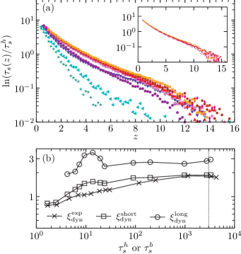
Figure 3: (Color online) (a) Self-overlap relaxation times in the KA system divided by value $\tau_{s}^{h}$, the value of $\tau_{s}(z)$ averaged over the large $z$ range $[15.4:15.8]$. The temperatures shown her are the same as in Fig. 1. The relaxation is exponential at high $T$, becomes very curved at intermediate temperature $T\approx 0.6$, and then evolves very little at low $T$. For all temperatures, there is an exponential decay at short distances, yielding a length $\xi^{\rm short}_{\rm dyn}$. There is also an approximately exponential decay at long distances from which we extract $\xi^{\rm long}_{\rm dyn}$. The inset isolates temperatures $0.432\leq T\leq 0.5$ to emphasize the low-$T$ saturation. (b) Relaxation time dependence of the three dynamic lengths extracted from fitting the profiles plotted against $\tau_{s}^{b}$ for $\xi_{\rm dyn}^{\rm exp}$ and $\tau_{s}^{h}$ for $\xi^{\rm long}_{\rm dyn}$ and $\xi^{\rm short}_{\rm dyn}$. The approximate position of $T_{c}$ is indicated by a vertical dotted line. Lengths are shown for all temperatures listed in Sec. II.

As an alternative approach for analyzing the data, we divide the profiles $\tau_{s}(z)$ by $\tau_{s}^{h}$, the value of the relaxation time measured at large $z$. We show the result in Fig. 3(a). There are several features worthy of discussion when viewed from this perspective. First, except for the highest temperatures, the curves are at $z_{max}$ still decaying which shows that the accuracy of our data allows us to see finite size effects in the dynamics even in the center of the box. Second, while the highest temperatures display exponential decay of $\ln(\tau_{s})$, the curves at the lowest temperatures are somewhat bent in this log-lin representation and it is not clear how to best analyze quantitatively this curvature. As a first attempt, we have tried to describe these data using an exponential decay at short $z$, followed by a second exponential decay at longer $z$. At intermediate supercooling, particularly at $T=0.6$, deviations from a single exponential decay are indeed quite pronounced. Third, the low $T$ curves nearly collapse (except perhaps at very large $z$ values). This is illustrated in the inset of Fig. 3(a) where the curves from the lowest five temperatures are isolated, clearly showing that these profiles are virtually identical over a large range of distances, despite the fact that relaxation times change by nearly two decades over that same temperature regime (see Fig. 1).

Since in this representation the data shows a clear curvature, we have chosen to split it into two parts, one for $z\leq z^{*}$ and one for $z>z^{*}$. From these fits we have extracted two dynamical length scales, $\xi_{\rm dyn}^{\rm short}$ and $\xi_{\rm dyn}^{\rm long}$, respectively. For $T>0.6$ best fits were obtained with $z^{*}=5$ and for $T\leq 0.6$ best fits resulted when using $z^{*}=6$. These lengths are shown in Fig. 3(b), along with the previous $\xi_{\rm dyn}^{\rm exp}$, for reference. We have also fit these data with a sum of exponentials, which provides a fit that matches the raw data quite well. Unfortunately the large number of fit parameters leads to overfitting that results in nonphysical length scales.

It is important to emphasize that even with this refined method of analysis, our previous results concerning the saturation of $\xi_{\rm dyn}^{\rm exp}$ remain robust. Clearly, even without any fitting, there is still a saturation of the dynamic profiles at temperatures close to $T_{c}$, as can be seen from the collapse of the data with the new normalization at low $T$ (see inset of Fig. 3(a)). This shows that the observation that $\xi_{\rm dyn}^{\rm exp}$ saturates as a function of $T$ does not depend on the detail how the length scale has been determined.

This more precise type of analysis permits to detect an unexpected feature in the $T-$dependence of the dynamic length scales. From Fig. 3(b) we see that the absolute value and the $T-$dependence of $\xi^{\rm short}_{\rm dyn}$ are very similar to the ones of $\xi_{\rm dyn}^{\rm exp}$ in that also this length scale grows with decreasing $T$ and then saturates around $T_{c}$. The $T-$dependence of $\xi^{\rm long}_{\rm dyn}$ is somewhat weaker than the one of $\xi^{\rm short}_{\rm dyn}$ in that it increases only by a factor of around 1.5 instead of the factor of two found for the latter. Much more important is, however, the observation that at intermediate temperatures, $T\approx 0.6$, $\xi^{\rm long}_{\rm dyn}$ shows a very pronounced peak. We stress that this peak is in no way a result of the fit and the behavior is clearly evident from inspection of the data in Fig. 3(a).

We note that this temperature is significantly above the mode-coupling temperature of the system, $T_{c}\sim 0.435$, but it coincides with the crossover temperature recently termed “$T_{s}$” in Ref. Flenner et al., 2014. The authors of Ref. Flenner et al., 2014 identify this $T_{s}$ both with the breakdown of the Stokes-Einstein relation as well as a change in the “shape” of dynamical heterogeneities. While a quantitative connection between $\xi_{\rm dyn}^{\rm long}$ and the Stokes-Einstein decoupling is a priori not obvious, we will in the following provide evidence that both types of behavior are indeed correlated.

We emphasize that the non-monotonic evolution of the length $\xi_{\rm dyn}^{\rm long}$ is a qualitatively different phenomenon from the evolution of a dynamic length discussed in Ref. Kob et al., 2012a. Indeed, because of the single exponential fitting protocol used in that paper, the analog crossover at temperature $T_{s}$ was previously not detected in the HARM system. In fact, while $\ln(\tau_{s})$ seems more exponential in the HARM system than in the KA system, we indeed see a signature of this higher temperature crossover around $T\approx 9$, near the putative $T_{s}$ for this model, a temperature not examined in Ref. Kob et al., 2012a (see Appendix C). In particular, it should be noted that fits to obtain $\xi_{\rm dyn}^{\rm exp}$ as shown in Fig. 2 and in Ref. Kob et al., 2012a give relatively little weight to the relaxation times at large $z$, thus making the peak seen in $\xi^{\rm long}_{\rm dyn}$ is hardly noticeable in $\xi_{\rm dyn}^{\rm exp}$ (see Fig. 3). Note that the discovery of this novel crossover phenomenon does not affect any of the conclusions about the dynamical length scale having a maximum at $T_{c}$ in this system because we find, as in the KA system, that $\xi_{\rm dyn}^{\rm exp}\approx\xi_{\rm dyn}^{\rm short}$, and both these length scales have indeed a maximum in the vicinity of the mode-coupling crossover temperature $T_{c}$.

To give further evidence for a relationship between the crossover temperature $T_{s}$ and the evolution of the length $\xi_{\rm dyn}^{\rm long}$, we have repeated our full analysis of dynamic profiles for a third model, namely the WCA system, which again shows this anomalous behavior around $T_{s}\approx 0.425$, as shown in Appendix C.

IV Comparison of transverse and longitudinal relaxation

In this section, we investigate the connection between dynamic profiles and the crossover temperature $T_{s}$ further. Because $T_{s}$ was previously related to a change in the geometry of dynamic heterogeneities Flenner et al. (2014), a possible connection could come from a geometric analysis of dynamic profiles near amorphous walls. To this end, we separately analyze the relaxation into perpendicular and parallel components with respect to the wall.

We analyze the self-intermediate scattering function at different distances from the wall, as defined in Eq. (3). It is simple to resolve the relaxation times for dynamics parallel and perpendicular to the wall, as done for instance in Ref. Scheidler et al., 2004. The relaxation times obtained for wavevectors parallel to the wall are shown in Fig. 1. Here, $\tau^{||}(z)$ has been divided by a constant value corresponding to the ratio $\tau^{||}(z)/\tau_{s}(z)$ at a single distance ($z\approx 15$) and a single temperature ($T=0.435$). The curves and points respectively representing $\tau^{||}(z)$ and $\tau_{s}(z)$ lie perfectly on top of each other except for a small deviation at the highest temperatures, suggesting that $\tau^{||}(z)$ reports on the same physics as $\tau_{s}(z)$ at supercooled temperatures, and does not contain additional physical information about relaxation near the amorphous wall.

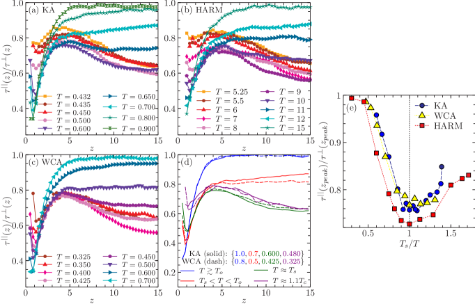
Figure 4: (Color online) (a-c) Distance dependence of the ratio of the parallel to perpendicular relaxation times in the three models studied. Due to the presence of the wall, $\tau^{||}(z)\leq\tau^{\perp}(z)$ at all distances. At high temperatures, the curves tends to unity but for lower temperatures the curves approach a fractional value for the $z$-range accessible. (d) Profiles of the curves in the distinct regimes identified, emphasizing in particular the emergence of a maximum in the ratio at a distance $z_{\rm peak}$. Results for KA are shown with solid lines and for WCA with dashed lines. At $z=15$, from top to bottom the curves are ordered $T\gtrsim T_{o}$, $T_{s}<T<T_{o}$, $T\approx 1.1T_{c}$, and $T\approx T_{s}$. (e) The ratio of relaxation times at $z_{\rm peak}$ as a function of $T_{s}/T$, showing that the peak value is minimized when $T\approx T_{s}$, the crossover temperature analyzed in Ref. Flenner et al., 2014. The values used for $T_{s}$ are 0.6, 9.0, and 0.425 for the KA, HARM and WCA systems, respectively.

In agreement with previous results Scheidler et al. (2004), the relaxation times obtained for wavevectors perpendicular to the wall are always slower than for those parallel to the wall. In Fig. 4(a-c) we show how the perpendicular relaxation times compare to the parallel relaxation times at different distances from the wall via the investigation of the ratio $\tau^{||}(z)/\tau^{\perp}(z)$ in the three different models studied in this work, the HARM, KA and WCA systems.

In each system three temperature regimes can be identified. The qualitative features of these regimes are illustrated by Fig. 4(d), where we select a subset of equivalent temperatures for each system, as being representative of the various regimes, which can be described as follows.

• Above $T_{o}$, the wall suppresses perpendicular more than parallel relaxation at small $z$, but then the ratio tends rapidly towards unity at large distances.

• Near $T_{o}$, the ratio tends to a pseudo-plateau at values less than one for all $z$ values accessible. A dip in the ratio of $\tau^{||}(z)/\tau^{\perp}(z)$ is also observed to develop near $z\approx 1$. This results in a maximum of the ratio at an intermediate distance $z_{\rm peak}\approx 4.0$ as $T$ is lowered.

• At temperatures below $T_{o}$, the curves become more complex in that at large $z$ the values of the ratio decreases whereas at $z_{\rm peak}$ the ratio is at intermediate $T$ basically constant before it increases slightly. Furthermore we see that the dip at $z\approx 1$ also rises slightly with decreasing temperature.

We define $z_{\rm peak}$ as the distance from the wall where the ratio $\tau^{||}/\tau^{\perp}$ peaks and consider the temperature evolution of this peak value, as shown in Fig. 4(e). In all three systems, the temperature where the peak value is minimized falls very close to values of $T_{s}$ given in Ref. Flenner et al., 2014.

This coincidence is robust against finite size effects that are known to affect the dynamics in simulation boxes with an elongated shape Coslovich and Kob (2014). Tests using larger box sizes demonstrate that the precise value of the ratio at large $z$ depends weakly on the box size, but the data up to $z_{\rm peak}$ and just beyond are fairly insensitive to such changes, as demonstrated in Appendix D. Hence the behavior and temperature correspondence appear to be fairly insensitive to finite size effects.

The precise dependence of the ratio $\tau^{||}(z)/\tau^{\perp}(z)$ is complicated, and further microscopic investigations of its behavior would be needed to understand these data in more detail. However, it is interesting to speculate on the connection between the behavior observed in Fig. 4(e) and that reported in Ref. Flenner et al., 2014. The authors of Ref. Flenner et al., 2014 note that the ratio of dynamical heterogeneity length scales associated with parallel and perpendicular displacements markedly changes behavior at $T_{s}$, which they claim to be the temperature at which violation of the Stokes-Einstein relation first occurs. The fact that we observe in the vicinity of $T_{s}$ a significant change in the $T-$dependence of $\tau^{||}(z)/\tau^{\perp}(z)$ is harmonious with the notion that this temperature is associated with a change in directionally resolved relaxation motifs, and gives further impetus for microscopic study of particle motion near the frozen wall as $T$ varies above and below $T_{s}$.

It should also be noted that we observe clear features of altered relaxation in both $\xi_{\rm dyn}^{\rm long}$ as well as $\tau^{||}(z)/\tau^{\perp}(z)$ at $T_{s}$, independent of metrics based on Stokes-Einstein violation, whose onset is not necessarily sharp enough to clearly define a characteristic temperature. In this sense, one can bypass definitions based on transport anomalies and relate $T_{s}$ directly to the change of two-point relaxation behavior provided by the proximity of a frozen interface.

In summary we can conclude that the results of this section and Sec. III above give further evidence in support of the notion, first advanced in Ref. Flenner et al., 2014, of a well-defined characteristic temperature $T_{s}$ below the onset temperature of slow dynamics but above $T_{c}$, which physically relates to a marked crossover in the geometric properties of dynamic heterogeneity.

V Discussion and Conclusions

In this work we have extended previous studies related to the relaxation of supercooled liquids near a wall created from a subset of particles fixed in their equilibrium positions. We find clear evidence that as $T_{c}$ is approached, the dynamical length scale defined in Refs. Kob et al., 2012a and Scheidler et al., 2002 quantitatively saturates in the KA system. This behavior is to be contrasted with the non-monotonic growth of the same length scale in the HARM system. This distinction, namely a saturation as opposed to a decrease in the length scale below $T_{c}$, is in harmony with both the behavior of $\chi_{4}^{NVE}$ Berthier et al. (2007); Flenner and Szamel (2013) as well as trends in the behavior of finite size effects as filtered through relaxation times in these two models Berthier et al. (2012). Taken together, these results all suggest that the crossover between transport mechanisms at $T_{c}$ is qualitatively similar in both systems, but is quantitatively sharper in the HARM, which may therefore be viewed to be closer to the idealized mean-field limit than the KA system.

We have also investigated the behavior of relaxation channels parallel and perpendicular to the wall. While motion parallel to the amorphous wall mirrors the behavior revealed by studies of the self-overlap function, we found that the behavior of the ratio $\tau^{||}(z)/\tau^{\perp}(z)$ shows clear evidence of a change in behavior at a recently identified temperature $T_{s}$, across three different model systems. In Ref. Flenner et al., 2014 it has been argued that $T_{s}$ marks a temperature where the shape of the dynamical heterogeneities changes, in the sense that transverse and longitudinal relative motions of particles become decoupled. Thus it is physically reasonable that close to the wall such a decoupling also affects the relaxation behavior in the parallel direction in a different manner than in the orthogonal one, thus rationalizing our findings regarding the $T-$ and $z-$dependence of $\tau^{||}(z)/\tau^{\perp}(z)$.

While our results place the change of transport mechanisms invoked to account for the dynamics of the HARM model Kob et al. (2012a, b) near an amorphous wall on firmer grounds, we emphasize that the strong saturation of the dynamic lengthscale $\xi_{\rm dyn}^{\rm exp}$ revealed in both HARM and KA models has no clear counterpart in available measurements of dynamic lengthscales from bulk four-point functions Flenner and Szamel (2012); Kob et al. (2012c), which appear to display no obvious saturation in the mode-coupling regime. Although this might indicate that both types of measurements are unrelated, we also note that the crossover temperature $T_{s}$ detected through analysis of four-point functions in Ref. Flenner et al., 2014 is also observed here using measurements near an amorphous wall via two-point quantities, albeit those extracted near an object that breaks spatial symmetry. While this approach is in the same spirit of earlier studies based on measurements of the response of two-point correlators to external fields Berthier et al. (2007, 2005), the present set-up using pinned particles provides a potentially simple means to observe the changes that occur at $T_{s}$ in an experimental setting. Future work should be devoted to real-space dynamical analysis of the behavior of motion parallel and perpendicular to the wall in order to gain deeper insight into the observations presented in this work. Overall, these results reveal that a better understanding of the connection between the various dynamic lengthscales studied in supercooled liquids is needed.

Appendix A Static Overlaps

Although the focus of this work is on the dynamical properties of the KA system near an amorphous wall, it is also useful to investigate the growth of static order. In Fig. 5 we show the static overlaps for comparison with Ref. Kob et al., 2012a. As in that work, we see that the static overlap decays exponentially with distance from the wall, and we remark that these static quantities decay much more quickly than the dynamical profiles shown in Figs. 3. We see a slight “layering” effect which we suspect is more pronounced here than in Ref. Kob et al., 2012a because in the present work we used a completely amorphous wall, while in Ref. Kob et al., 2012a a reflective wall and an amorphous potential were used in combination.

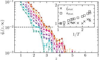
Figure 5: (Color online) Static overlap values extracted from $q_{c}(z,t\to\infty)$ for the temperatures in Fig. 1. The decay is exponential and becomes steadily longer ranged as temperature is lowered. Two static length scales, $\xi_{\rm stat}$, the inverse of the slope of the decay, and $a_{\rm stat}$, the $z$ value where $\tilde{q}_{c}(z,\infty)$ lines cross the value $C=0.01$, as illustrated by a horizontal dashed line may be extracted. $1\sigma$ error bars from a bootstrap analysis are shown Efron and Tibshirani (1993). Inset: The lengths $\hat{a}_{\rm stat}=a_{\rm stat}/a_{\rm stat}^{0}$ and $\hat{\xi}_{\rm stat}=\xi_{\rm stat}/\xi_{\rm stat}^{0}$ where $a_{\rm stat}^{0}$=1.92 and $\xi_{\rm stat}^{0}$=0.56 are the values of the lengths at high temperature, $T=0.9$.

To extract static length scales, we choose to fit these curves to the function

$$\tilde{q}_{c}(z,\infty)=C\exp(-(z-a_{\rm stat})/\xi_{\rm stat}),$$ (5)

with a fixed value of $C=0.01$, shown by a horizontal dashed line in Fig. 5. This fit gives values for $\xi_{\rm stat}$ describing the exponential decay of the static profiles, which are small and grow very slowly. In addition, we can consider the evolution of $a_{\rm stat}$ quantifying the distance $z$ for which the overlap equals $C=0.01$. This is another static length scale, which is slightly larger than $\xi_{\rm stat}$ and also grows quite slowly.

Both are shown in the inset of Fig. 5 and are seen to grow by a much smaller amount than the dynamical length scales measured. Although there are small qualitative differences between the KA and HARM systems with respects to the magnitudes of static and dynamic length scales, both show a pronounced decoupling between static and dynamic properties, in line with other studies showing static length scales which are smaller and grow more slowly than dynamical ones Karmakar et al. (2009); Berthier and Kob (2012); Hocky et al. (2012); Charbonneau and Tarjus (2013).

Appendix B Relaxation times in the KA system

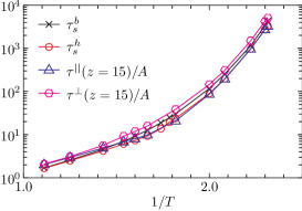
Figure 6: (Color online) Temperature dependence of the various relaxation times discussed in the main text for the KA system. The values of $\tau^{||}$ and $\tau^{\perp}$ have been scaled by the value $A=0.7$ as discussed in Fig. 1.

Fig. 6 compares the four relaxation times used in the main text for the KA system. As discussed previously, the values of $\tau^{||}(z)$ and $\tau_{s}(z)$ can be scaled on top of each other using a temperature independent constant, although there is some deviation at high temperatures. The need for rescaling simply arises because of the choice of the window size $l=0.45$ for the self-overlap calculation and the value $k=7.25$ for the self-intermediate scattering function. In Fig. 6, we have also rescaled the values of $\tau^{\perp}$ showing that relaxation in the perpendicular direction in the middle of the box is slower than in the parallel direction at all temperatures. Finally, we also show the value of the self-overlap relaxation time without the wall, which is larger than the self-overlap relaxation time at all temperatures at the center of the box in the presence of the wall. This origin of this result will be discussed in a forthcoming work Coslovich and Kob (2014).

Appendix C Overlap curves in the HARM and WCA systems

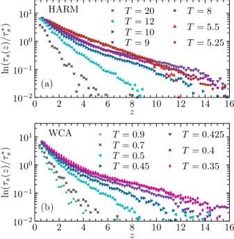
Figure 7: (Color online) Distance dependence of the self-overlap relaxation times for the HARM system (a) and the WCA system (b) in a representation similar to the one of Fig. 3 for the KA model.

For the sake of comparison with the results presented in Fig. 3, we also include the results for the HARM and WCA systems. In Fig. 7(a) the results for the HARM system are plotted. While the curves decay in a completely exponential manner at the highest and lowest temperatures, there is a pronounced curvature or double-exponential character near $T=9$, a temperature not studied in Ref. Kob et al., 2012a. The curvature at $T=8$ is consistent with the data in that work.

Figure 7(b) shows results for the WCA system. Here again the data appears to have double exponential character starting near $T=0.425$. We note for both models that this behavior occurs in the range identified as $T_{s}$ by Ref. Flenner et al., 2014. A more extensive study should test whether there is any difference using a smoothed WCA potential, which has slightly different dynamical properties at low temperatures from those of the standard WCA (see e.g. Ref. Coslovich, 2011).

Appendix D Finite Size Effects

Figure 8: (Color online) Ratio of parallel to perpendicular relaxation times in three different box sizes. The size used in the main text is indicated by a solid line, while data for a larger box size is shown with dotted lines, and for a smaller box at $T=0.6$ by a dashed line, showing that finite size effects do not affect the crossover behavior at $T=T_{s}$ discussed in Sec. IV.

We have performed additional simulations to check that our conclusions are robust with respect to changes in system sizes. As an example of such tests, we consider the behavior of the ratio of perpendicular and parallel relaxation times for the KA system shown in Fig. 4(a).

In Fig. 8 we show the same calculation for the KA system using $N=7600$ in a box with aspect ratio $1:1:4$. We also show at $T=T_{s}=0.6$ the behavior for the $N=5700$ system in an effectively smaller box, generated by freezing a wall of thickness $W=9$ rather than $W=3$ as in the main body of this article. While the large-$z$ behavior seems to depend on the system size, the data up to $z_{\rm peak}$ appear to be independent of the box size considered. Hence we conclude that our approach to analyze the data in Fig. 4(e) to define $T_{s}$ is safe, and that the existence of a correspondence between the crossover $T_{s}$ of Ref. Flenner et al., 2014 and the present comparative study of parallel and perpendicular relaxation times is a robust finding.

Finally, we note that the large-$z$ values of these data change with system size. We believe that this is due to complex hydrodynamic coupling between the dynamics in the two directions. In fact, we found in the bulk that for $T<T_{o}$ in a non-cubic box, the ratio of $\tau^{||}(z)/\tau^{\perp}(z)$ is non-unity due to hydrodynamic effects (data not shown). For example, in the KA system, this ratio is approximately 0.85 for a $3:1:1$ box at temperatures $T\leq 0.8$. Study of the precise origin of this phenomenon is beyond the scope of this work and will require further investigation.

References

- Biroli et al. (2008) G. Biroli, J.-P. Bouchaud, A. Cavagna, T. S. Grigera, and P. Verrocchio, Nature Phys. 4, 771 (2008).
- Kim et al. (2009) K. Kim, K. Miyazaki, and S. Saito, Europhys. Lett. 88, 36002 (2009).
- Kob et al. (2012a) W. Kob, S. Roldán-Vargas, and L. Berthier, Nature Phys. 8, 164 (2012a).
- Jack and Berthier (2012) R. L. Jack and L. Berthier, Phys. Rev. E 85, 021120 (2012).
- Karmakar et al. (2012) S. Karmakar, E. Lerner, and I. Procaccia, Physica A 391, 1001 (2012).
- Berthier and Kob (2012) L. Berthier and W. Kob, Phys. Rev. E 85, 011102 (2012).
- Charbonneau et al. (2012) B. Charbonneau, P. Charbonneau, and G. Tarjus, Phys. Rev. Lett. 108, 035701 (2012).
- Hocky et al. (2012) G. M. Hocky, T. E. Markland, and D. R. Reichman, Phys. Rev. Lett. 108, 225506 (2012).
- Charbonneau and Tarjus (2013) P. Charbonneau and G. Tarjus, Phys. Rev. E 87, 042305 (2013).
- Kob and Berthier (2013) W. Kob and L. Berthier, Phys. Rev. Lett. 110, 245702 (2013).
- Jack and Fullerton (2013) R. L. Jack and C. J. Fullerton, Phys. Rev. E 88, 042304 (2013).
- Bouchaud and Biroli (2004) J.-P. Bouchaud and G. Biroli, J. Chem. Phys. 121, 7347 (2004).
- Cammarota et al. (2011) C. Cammarota, G. Biroli, M. Tarzia, and G. Tarjus, Phys. Rev. Lett. 106, 115705 (2011).
- Scheidler et al. (2002) P. Scheidler, W. Kob, and K. Binder, Europhys. Lett. 59, 701 (2002).
- Kim (2003) K. Kim, Europhys. Lett. 61, 790 (2003).
- Kob et al. (2012b) W. Kob, S. Rold́an-Vargas, and L. Berthier, Physics Procedia 34, 70 (2012b).
- Kob and Coslovich (2014) W. Kob and D. Coslovich, arXiv:1403.3519 (2014).
- Stevenson et al. (2006) J. D. Stevenson, J. Schmalian, and P. G. Wolynes, Nature Phys. 2, 268 (2006).
- Berthier and Biroli (2011) L. Berthier and G. Biroli, Rev. Mod. Phys. 83, 587 (2011).
- Berthier et al. (2007) L. Berthier, G. Biroli, J.-P. Bouchaud, W. Kob, K. Miyazaki, and D. R. Reichman, J. Chem. Phys. 126, 184503 (2007).
- Kim et al. (2013) K. Kim, S. Saito, K. Miyazaki, G. Biroli, and D. R. Reichman, J. Phys. Chem. B 117, 13259 (2013).
- Berthier et al. (2012) L. Berthier, G. Biroli, D. Coslovich, W. Kob, and C. Toninelli, Phys. Rev. E 86, 031502 (2012).
- Flenner and Szamel (2013) E. Flenner and G. Szamel, J. Chem. Phys. 138, 12A523 (2013).
- Kob and Andersen (1995) W. Kob and H. C. Andersen, Phys. Rev. E 51, 4626 (1995).
- Kob (1999) W. Kob, J. Phys. Condens. Matter 11, R85 (1999).
- Berthier and Tarjus (2010) L. Berthier and G. Tarjus, Phys. Rev. E 82, 031502 (2010).
- Plimpton (1995) S. Plimpton, J. Comp. Phys. 117, 1 (1995), URL http://lammps.sandia.gov.
- Weeks et al. (1971) J. D. Weeks, D. Chandler, and H. C. Andersen, J. Chem. Phys. 54, 5237 (1971).
- O’Hern et al. (2002) C. S. O’Hern, S. A. Langer, A. J. Liu, and S. R. Nagel, Phys. Rev. Lett. 88, 075507 (2002).
- Berthier and Witten (2009) L. Berthier and T. A. Witten, Europhys. Lett. 86, 10001 (2009).
- Efron and Tibshirani (1993) B. Efron and R. Tibshirani, An introduction to the bootstrap, vol. 57 of Monographs on statistics and applied probability (Chapman & Hall/CRC, 1993).
- Flenner et al. (2014) E. Flenner, H. Staley, and G. Szamel, Phys. Rev. Lett. 112, 097801 (2014).
- Scheidler et al. (2004) P. Scheidler, W. Kob, and K. Binder, J. Phys. Chem. B 108, 6673 (2004).
- Coslovich and Kob (2014) D. Coslovich and W. Kob, to be published (2014).
- Flenner and Szamel (2012) E. Flenner and G. Szamel, Nature Physics 8, 696 (2012).
- Kob et al. (2012c) W. Kob, S. Roldán-Vargas, and L. Berthier, Nature Physics 8, 697 (2012c).
- Berthier et al. (2005) L. Berthier, G. Biroli, J.-P. Bouchaud, L. Cipelletti, D. El Masri, D. L’Hôte, F. Ladieu, and M. Pierno, Science 310, 1797 (2005).
- Wilde et al. (2011) M. Wilde, M. Hategan, J. M. Wozniak, B. Clifford, D. S. Katz, and I. Foster, Parallel Comput. 37, 633 (2011).
- Karmakar et al. (2009) S. Karmakar, C. Dasgupta, and S. Sastry, Proc. Natl. Acad. Sci. 106, 3675 (2009).
- Coslovich (2011) D. Coslovich, Phys. Rev. E 83, 051505 (2011).