Detecting floating black holes as they traverse the gas disk of the Milky Way

Abstract

A population of intermediate-mass black holes (BHs) is predicted to be freely floating in the Milky Way (MW) halo, due to gravitational wave recoil, ejection from triple BH systems, or tidal stripping in the dwarf galaxies that merged to make the MW. As these BHs traverse the gaseous MW disk, a bow shock forms, producing detectable radio and mm/sub-mm synchrotron emission from accelerated electrons. We calculate the synchrotron flux to be $\sim\rm 0.01-10\,mJy$ at GHz frequency, detectable by Jansky Very Large Array, and $\sim 10-100\,\mu\rm Jy$ at $\sim 10^{10}-10^{12}\,\rm Hz$ frequencies, detectable by Atacama Large Millimeter/sub-millimter Array. The discovery of the floating BH population will provide insights on the formation and merger history of the MW as well as on the evolution of massive BHs in the early Universe.

1 Introduction

Galaxies grow through accretion and hierarchical mergers. During the final phase of the merger of two central black holes, anisotropic emission of gravitational waves (GW) kicks the BH remnant with a velocity up to a few hundreds $\rm km\,s^{-1}$ (Baker et al. 2006; Campanelli et al. 2007; Blecha & Loeb 2008). Additionally, BHs can be ejected from triple systems (Kulkarni & Loeb 2012; Hoffman & Loeb 2007), or result from tidally-stripped cores of dwarf galaxies (Bellovary et al. 2010). For GW recoils, the typical kick velocity is large enough for the BHs to escape the shallow gravitational potential of low-mass galaxies, but smaller than the escape velocity of the MW halo. This is also the case for triple systems as long as the kick velocity is $<500\,\rm km\,s^{-1}$. Consequently, a population of floating BHs formed from mergers of low-mass galaxies are trapped in the region that eventually makes the present-day MW (Madau & Quataert 2004; Volonteri & Perna 2005; Libeskind et al. 2006). Previous studies suggested that more than $\sim$ 100 floating BHs should be in the halo today, based on a large statistical sample of possible merger tree histories for the MW halo today (O’Leary & Loeb 2009, 2012). This population of recoiled BHs is supplemented by BHs from tidally disrupted satellites of the MW (Bellovary et al. 2010). The discovery of this BH population will provide constraints on the formation and merger history of the MW as well as the dynamical evolution of massive BHs in the early Universe.

It has been proposed that a compact cluster of old stars from the original host galaxies is carried by each floating BH (O’Leary & Loeb 2009). In this Letter, we propose an additional observational signature of floating BHs, using the MW gas disk as a detector. As the BHs pass through the MW disk supersonically they generate a bow shock, which results in synchrotron radiation detectable at radio and mm/sub-mm frequencies.

The paper is organized as follows. In § 2, we discuss the interaction between BHs and the gas in the MW disk. In § 3, we calculate the synchrotron radiation from the bow shocks produced as the BHs cross the MW disk, and discuss the detectability of this radiation. Finally, in § 4, we summarize our results and discuss their implications.

2 Interaction between a floating black hole and the MW disk gas

We consider a BH moving at a speed $V_{\bullet}$ relative to the interstellar medium (ISM) of number density $n_{{}_{\rm ISM}}$. The effective radius of influence of the moving black hole is given by the Bondi accretion radius:

$$R_{\rm Bondi}=\frac{GM_{\bullet}}{c_{\rm s}^{2}+V_{\bullet}^{2}}\approx\frac{GM_{\bullet}}{V_{\bullet}^{2}}=0.01\,M_{5}\,V_{200}^{-2}\;\rm pc\;,$$ (1)

where $G$ is Newton’s constant, $M_{5}=\left(M_{\bullet}/10^{5}M_{\odot}\right)$ and $V_{200}=\left(V_{\bullet}/200\,\rm km\,s^{-1}\right)$. The sound speed $c_{\rm s}$ of hydrogen in the ISM is given by $c_{\rm s}=\left(\Gamma P/\rho\right)^{1/2}=11.7\,T_{4}^{1/2}\,\rm km\,s^{-1}$, where $\Gamma=5/3$ is the adiabatic index and $T_{4}=\left(T/10^{4}\,\rm K\right)$. In the case of a supersonic shock with velocity $V_{\rm sh}\gg c_{\rm s}$, the total mass enclosed within the Bondi radius is given by $\Delta M_{\rm ISM}=1.3\times 10^{-7}\,M_{5}^{3}\,V_{200}^{-6}\,n_{0}\;M_{\odot}$, where $n_{0}=\left(n_{{}_{\rm ISM}}/10^{0}\,\rm cm^{-3}\right)$. The rate of fresh mass being shocked in the ISM is $\Delta\dot{M}_{\rm ISM}=3.7\times 10^{-9}\,M_{5}^{2}\,V_{200}^{-3}\,n_{0}\;M_{\odot}\,\rm yr^{-1}$. The total kinetic power can be expressed as,

$$\begin{split}L_{\rm kin}&=\frac{1}{2}\left(2\pi R_{\rm Bondi}^{2}n_{{}_{\rm ISM}}m_{\rm p}V_{\bullet}\right)V_{\bullet}^{2}\\ &=4.7\times 10^{31}M_{5}^{2}\,V_{200}^{-1}\,n_{0}\;\rm erg\,s^{-1}\;,\end{split}$$ (2)

where $m_{\rm p}$ is the proton mass.

3 Observational appearance

As a floating BH travels through the MW disk supersonically, a bow shock is formed with a half opening angle $\theta\sim\mathcal{M}^{-1}$ (Shu 1992; Kim & Kim 2009), where the Mach number is given by $\mathcal{M}=V_{\bullet}/c_{\rm s}\approx 17.0\,V_{200}\,T_{4}^{-1/2}$ (see Fig.1). The electrons accelerated in the shock produce non-thermal radiation that can be detected.

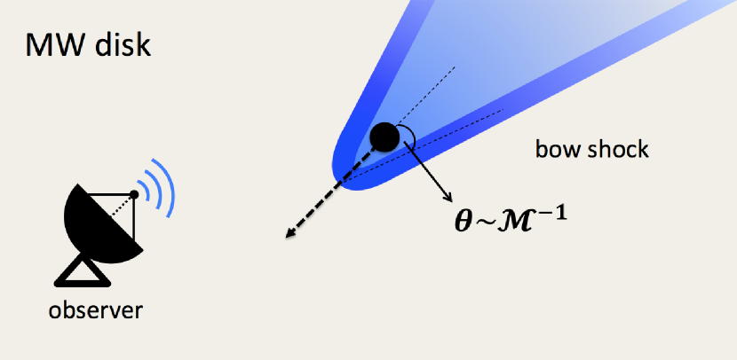
Figure 1: Sketch of the bow shock geometry around a BH crossing the gaseous MW disk.

3.1 Non-thermal spectrum

3.1.1 Single electron

Next, we calculate synchrotron emission from the shock accelerated electrons around the BH. We adopt $n_{0}=1$ and $T_{4}=1$ in the numerical examples that follow. From the Rankine-Hugoniot jump conditions for a strong shock the density of the shocked gas is $n_{\rm s}\approx\left(\Gamma+1\right)\,n_{{}_{\rm ISM}}/\left(\Gamma-1\right)=4\,n_{{}_{\rm ISM}}$, whereas its temperature is, $T_{\rm s}=[(\Gamma+1)+2\Gamma(\mathcal{M}^{2}-1)][(\Gamma+1)+(\Gamma-1)(\mathcal{M}^{2}-1)]T/(\Gamma+1)^{2}\mathcal{M}^{2}$. The magnetic field can by obtained by assuming a near-equipartition of energy $U_{\rm B}=B^{2}/8\pi=\xi_{\rm B}\,n_{\rm s}\,kT_{\rm s}$, where $\xi_{\rm B}$ is the fraction of thermal energy carried by the magnetic field. Thus, the magnetic field behind the shock is given by

$$B\approx 35\,\xi_{\rm B,-1}^{1/2}\,n_{0}^{1/2}\,T_{4}^{1/2}\;\mu\rm G\;,$$ (3)

where $\xi_{\rm B,-1}=\left(\xi_{\rm B}/0.1\right)$. We adopt $\xi_{\rm B,-1}=1$ in what follows in analogy with supernova (SN) remnants (Chevalier 1998).

For a single electron with Lorentz factor $\gamma$, the peak of its synchrotron radiation is at a frequency $\nu_{\rm syn}=4.2\,B_{-5}\,\gamma_{4}^{2}\;\rm GHz$, where $\gamma_{4}=\left(\gamma/10^{4}\right)$ and $B_{-5}=\left(B/10^{-5}\,\rm G\right)$. The total emitted power per unit frequency is given by (Rybicki & Lightman 1979)

$$P(\nu)=\frac{\sqrt{2}\,e^{3}B}{m_{\rm e}c^{2}}F(x)\;,$$ (4)

where $F(x)\equiv x\int^{\infty}_{x}K_{5/3}(\xi)\,d\xi$, $K_{5/3}(x)$ is the modified Bessel function of $5/3$ order, $x=\nu/c_{1}B\gamma^{2}$, $c_{1}=\sqrt{6}\,e/4\pi m_{\rm e}c$, $c$ is the speed of light and $m_{\rm e}$, $e$ are the electron mass and charge respectively. The pitch angle is assumed to be uniformly distributed.

The total power from synchrotron emission of a single electron is given by (Rybicki & Lightman 1979)

$$P_{\rm syn}=\frac{4}{9}r_{\rm 0}^{2}c\beta^{2}\gamma^{2}B^{2}=2.5\times 10^{-18}B_{-5}\,\nu_{{}_{\rm GHz}}\;\rm erg\,s^{-1}\;,$$ (5)

where $r_{\rm 0}=e^{2}/m_{\rm e}c^{2}$ is the classical radius of the electron and $\nu_{{}_{\rm GHz}}=\left(\nu_{\rm syn}\rm/GHz\right)$. We estimate the cooling time to be $t_{\rm cool}=\gamma mc^{2}/P_{\rm syn}=5.0\times 10^{7}B_{-5}^{-3/2}\nu_{{}_{\rm GHz}}^{-1/2}\;\rm yr$ for $V_{200}=1$. Since most of the emission is near the head of the Mach cone, we compare the cooling timescale with the dynamical timescale, which is given by $t_{\rm dyn}=R_{\rm Bondi}/V_{\bullet}\approx 53\,M_{5}V_{200}^{-3}\;\rm yr$. For the emission frequencies of interest, the cooling time is much longer than the lifetime of the shock.

3.1.2 Power-law distribution of electrons

Next we consider a broken power law distribution of electrons generated via Fermi acceleration:

$$N(\gamma)\,d\gamma=K_{0}\gamma^{-p}\left(1+\frac{\gamma}{\gamma_{\rm b}}\right)^{-1}\;(\gamma_{\rm min}\leq\gamma\leq\gamma_{\rm max}),$$ (6)

where $K_{0}$ is the normalization factor in electron density distribution, $p$ is the electron power law distribution index, and $\gamma_{\rm b}$, $\gamma_{\rm min}$, $\gamma_{\rm max}$ are the break, minimum and maximum Lorentz factor respectively. The break in the power law is due to synchrotron cooling. The total synchrotron power can be written as,

$$\begin{split}L_{\rm nt}&=\epsilon_{\rm nt}L_{\rm kin}=\int^{\gamma_{\rm max}}_{\gamma_{\rm min}}P_{\rm syn}N(\gamma)\,d\gamma\\ &=2.3\times 10^{30}\epsilon_{\rm nt,5}\,M_{5}^{2}\,V_{200}^{-1}\,n_{0}\;\rm erg\,s^{-1}\;,\end{split}$$ (7)

where $\epsilon_{\rm nt,5}=(\epsilon_{\rm nt}/5\%)$ is the fraction of electrons accelerated to produce non-thermal radiation. The normalization constant $K_{0}$ is obtained from the relation $K_{0}=L_{\rm nt}/\int^{\gamma_{\rm max}}_{\gamma_{\rm min}}P_{\rm syn}\gamma^{-p}\,d\gamma$. Observations imply that the ISM density distribution in the MW disk midplane can be roughly described by the form (Spitzer 1942; Kalberla & Kerp 2009),

$$n_{{}_{\rm ISM}}(r,z)=n_{\rm c}e^{-(r-R_{\odot})/R_{\rm n}}{\rm sech}^{2}\left[\frac{z}{\sqrt{2}z_{0}(r)}\right]\;,$$ (8)

where $r$ and $z$ are the radial and vertical coordinates relative to the disk midplane, $n_{\rm c}=0.9\,\rm cm^{-3}$, $R_{\rm n}=3.15\,\rm kpc$ and $z_{0}(r)$ is the scale height at $r$, given by $z_{0}(r)=h_{0}\,e^{(r-R_{\odot})/r_{0}}$ with $h_{0}=0.15\,\rm kpc$, $R_{\odot}=8.5\,\rm kpc$ and $r_{0}=9.8\,\rm kpc$ (Kalberla & Kerp 2009). The gas density and non-thermal luminosity as a function of radius in the MW disk midplane are shown in Figure 2.

Figure 2: Gas density, $n_{{}_{\rm ISM}}(z=0)$, and non-thermal luminosity in units of $10^{30}\epsilon_{\rm nt,5}M_{5}^{2}\,V_{200}^{-1}\,n_{0}$ in the midplane of the MW disk.

The electron acceleration time scale is given by $t_{\rm acc}=\xi_{\rm acc}\gamma m_{\rm e}c^{3}/eBV_{\bullet}^{2}$, where $\xi_{\rm acc}$ is a dimensionless constant of order unity (Blandford & Eichler 1987). The upper limit of the Lorentz factor $\gamma_{\rm max}$ can be obtained by equaling the acceleration and cooling timescale of electrons, $t_{\rm acc}=t_{\rm cool}$, giving

$$\gamma_{\rm max}=\frac{3m_{\rm e}cV_{\bullet}}{2\,\xi_{\rm acc}^{1/2}B^{1/2}e^{3/2}}=2.5\times 10^{7}\;V_{200}\,B_{-5}^{-1/2}\;.$$ (9)

Since the time the gas stays in the shocked region for the electrons to be accelerated is roughly the dynamical timescale, an additional constraint on $\gamma_{\rm max}$ can be obtained by equating the acceleration timescale of electrons and the dynamical time, $t_{\rm acc}=t_{\rm dyn}$, giving

$$\gamma_{\rm max}=\frac{eBV_{\bullet}R_{\rm Bondi}}{\xi_{\rm acc}m_{\rm e}c^{3}}=1.2\times 10^{5}\,B_{-5}M_{5}V_{200}^{-1}\;.$$ (10)

We will adopt this tighter constraint on $\gamma_{\rm max}$ in the following calculation. The emission frequency associated with $\gamma_{\rm max}$ is $\nu_{\rm max}=3\,\gamma_{\rm max}^{2}eB/4\pi m_{\rm e}c=4.2\times 10^{11}\,B_{-5}\gamma_{\rm max,5}^{2}\,\rm Hz$, where $\gamma_{\rm max,5}=(\gamma_{\rm max}/10^{5})$. The break Lorentz factor can be obtained by equaling the cooling and the dynamical time, giving $\gamma_{\rm b}=5.0\times 10^{9}B_{-5}^{-2}\,M_{5}^{-1}V_{200}^{3}$ and the corresponding frequency $\nu_{\rm b}=4.2\times 10^{10}\,B_{-5}\gamma_{\rm b,9}^{2}\rm\,GHz$, where $\gamma_{\rm b,9}=(\gamma_{\rm b}/10^{9})$. The value of $\nu_{\rm b}$ is above the frequency range of interest here and does not affect the observable synchrotron spectrum.

The emissivity and absorption coefficients are given by (Rybicki & Lightman 1979)

$$j_{\nu}=c_{2}B\int^{\gamma_{\rm max}}_{\gamma_{\rm min}}F(x)N(\gamma)\,d\gamma\;,$$ (11)

$$\alpha_{\nu}=-c_{3}B\frac{1}{\nu^{2}}\int^{\gamma_{\rm max}}_{\gamma_{\rm min}}\gamma^{2}\frac{d}{d\gamma}\left[\frac{N(\gamma)}{\gamma^{2}}\right]F(x)\,d\gamma\;,$$ (12)

where $c_{2}=\sqrt{2}e^{3}/4\pi m_{\rm e}c^{2}$ and $c_{3}=\sqrt{2}e^{3}/8\pi m_{\rm e}^{2}c^{2}$. From the radiative transfer equation, the specific intensity is given by (Rybicki & Lightman 1979)

$$I_{\nu}=\frac{j_{\nu}}{\alpha_{\nu}}\left(1-e^{-\tau_{\nu}}\right)\;,$$ (13)

where $\tau_{\nu}$ is the optical depth. The synchrotron luminosity and corresponding flux at a distance $d=10\;\rm kpc$ from the observer are plotted in Figure 3.

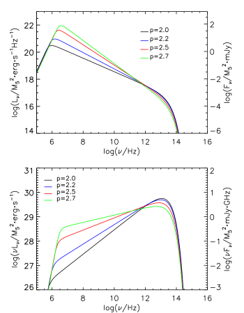
Figure 3: Synchrotron power and flux from non-thermal electrons accelerated by the bow shock of floating BHs, in units of $M_{5}^{2}$, for $n_{0}=1$, $V_{200}=1$, $L_{\rm nt}=3.0\times 10^{30}\;\rm erg\,s^{-1}$, $B_{-5}=3.5$, $\gamma_{\rm min}\sim 1$ and $\gamma_{\rm max}\sim 4.2\times 10^{5}$. The upper panel shows synchrotron flux while the lower panel shows the corresponding power. The left label of the vertical axis marks synchrotron luminosity per unit frequency (upper panel) or power per $\log\nu$ (lower panel) while the right one marks the corresponding flux at a distance of $d=10\rm\;kpc$. The black, blue, red and green lines correspond to power-law indices $p=2.0,\;2.2,\;2.5,\;2.7$ respectively in the electron energy distribution. Synchrotron self-absorption is significant at a frequency $\leq\rm\,MHz$ and the cooling break corresponds to a frequency $\sim 10^{19}\rm\,Hz$, which are outside the frequency range of interest.

3.2 Emission from the vicinity of the BH

Next we estimate the emission from the vicinity of the BH through a hot accretion flow (Narayan & Yi 1994). The Bondi accretion rate is given by $\dot{M}_{\rm Bondi}=9.1\times 10^{17}M_{5}^{2}\,n_{0}V_{200}^{-3}\;\rm g\,s^{-1}$ (Armitage & Natarajan 1999), and the Eddington accretion rate can be expressed as $\dot{M}_{\rm Edd}=L_{\rm Edd}/0.1c^{2}=1.39\times 10^{23}\,M_{5}\;\rm g\,s^{-1}$. We estimate the total luminosity in a radiatively inefficient accretion flow (RIAF) as,

$$L_{\bullet}=\eta\dot{M}c^{2}=5.4\times 10^{31}\zeta_{-1}^{2}\,M_{5}^{3}\,n_{0}^{2}\,V_{200}^{-6}\;\rm erg\,s^{-1}\;,$$ (14)

where $\eta\approx 0.1\left(\dot{M}/0.1\dot{M}_{\rm Edd}\right)$ is the efficiency of converting matter to radiation for $\dot{M}\leq 0.1\dot{M}_{\rm Edd}$ (Narayan & McClintock 2008) and $\zeta=\dot{M}/\dot{M}_{\rm Bondi}=10\,\zeta_{-1}$ is the accretion rate in units of $\dot{M}_{\rm Bondi}$. The BH accretion would produce X-ray emission which is not expected from the bow shock spectrum in Fig.3. Since $L_{\bullet}\propto M_{5}^{3}$, the accretion luminosity from interstellar medium accretion onto stellar mass BHs is negligible compared to our souce (Fujita 1998).

It is possible that an outflow would be formed near the BH. The outflow would produce a shock at a radius $R_{\rm out}$, which can be obtained from $f\dot{M}=\dot{M}_{\rm out}=4\pi R_{\rm out}^{2}n_{{}_{\rm ISM}}m_{\rm p}V_{\rm out}$, where $f\leq 1$ is the fraction of the inflowing mass channelled into the outflow. This gives,

$$\begin{split}R_{\rm out}&=\left(\frac{f\dot{M}}{4\pi n_{{}_{\rm ISM}}m_{\rm p}V_{\rm out}}\right)^{1/2}\\ &=6.8\times 10^{-4}\,f^{1/2}\zeta_{-1}^{1/2}M_{5}V_{200}^{-3/2}V_{\rm out,4}^{-1/2}\;\rm pc\;,\end{split}$$ (15)

where $V_{\rm out,4}=(V_{\rm out}/10^{4}\,\rm km\,s^{-1})$ is the velocity of the outflow. For typical parameters, we find that the outflow would be bounded with $R_{\rm out}\leq R_{\rm Bondi}$.

3.3 Observational signatures and detectability

Observationally, the BH emission cone would appear arc-shaped, with an angular diameter $\theta=R_{\rm Bondi}/d=0.22\,d_{1}^{-1}M_{5}V_{200}^{-2}\,\rm arcsec$, where $d_{1}=\left(d/10\,\rm kpc\right)$. The non-thermal radiation should be detectable at radio and mm/sub-mm bands. At a frequency $\nu\sim 1\rm\,GHz$, the synchrotron flux at a distance of $10\rm\,kpc$ is of order $0.01-10\rm\,mJy$, depending on the choice of $p$. This flux is detectable with the Jansky Very Large Array (JVLA), which has a complete frequency coverage from $1-50$ GHz, with a sensitivity of $\sim 5.5\,\mu\rm Jy/beam$ in a 1-hour integration and a signal to noise ratio $\rm S/N=1$ at $1-2$ GHz (Perley et al. 2011). At a frequency $\nu\sim 10^{10}-10^{12}\rm\,Hz$ in the mm/sub-mm band, the synchrotron flux at a distance of $10\rm\,kpc$ is of order $10-100\,\mu\rm Jy$, which is detectable by the Atacama Large Millimeter/sub-millimeter Array (ALMA), covering a wavelength range of $0.3-9.6\rm\,mm$, with an integration time of roughly $10^{4}\rm\,s$.

Morphologically, it is possible to distinguish the bow shock emission from other radio sources such as SN remnants or HII regions. The bow shock emission is elongated along the direction of the BH’s motion, whereas SN remnants would appear roughly circular on the sky. There are hundreds of cometary HII regions produced by a combination of supersonic motion of an OB-type star through dense gas and ionization of gas down a density gradient (Cyganowski et al. 2003; Immer et al. 2014). The Mach cone’s opening angle can be used to distinguish them from the much faster floating BHs. The ongoing survey of the Galactic plane with JVLA (NRAO 2014) has the potential to separate out these HII regions. There are far fewer confusing HII region sources at larger radius in the disk. Other high-velocity sources are pulsar wind nebulae (Gaensler 2005), hyper-velocity stars (Brown et al. 2006) and runaway stars (del Valle & Romero 2012; del Valle et al. 2013). The first type can be distinguished by observing the pulsar as well as its X-ray emission. The last two types produce less synchrotron radiation (del Valle & Romero 2012; del Valle et al. 2013), and thus can be distinguished as well. Globular clusters crossing the MW disk produce another class of contaminants. Their velocity relative to the disk is much larger than the velocity dispersion of their stars, so their Bondi radius is much smaller than their size. Thus, they should not produce significant synchrotron emission. The floating BHs are also embedded in a star cluster, but the cluster size is more compact and its gravity is dominated by the central BH (O’Leary & Loeb 2009, 2012).

4 Summary and discussion

If a floating BH happens to pass through the MW disk, then the non-thermal emission from the accelerated electrons in the bow shock around the BH should produce detectable signals in the radio and mm/sub-mm bands. The radio flux $\sim 0.01-10\;\rm mJy$ is detectable by JVLA, while the mm/sub-mm flux $\sim 10-100\,\mu\rm Jy$ is detectable by ALMA.

The density distribution of floating BHs in the MW has been studied by O’Leary & Loeb (2009, 2012) and by Rashkov & Madau (2014). High resolution simulations show that there is a BH of mass $\sim 2\times 10^{5}M_{\odot}$ within a few kpc from the Galactic center (Rashkov & Madau 2014).

Observations of the Galactic disk can be used to infer $n_{0}$ and $T_{4}$. The BH speed $V_{\bullet}$ can then be estimated from the Mach cone angle. The maximum Lorentz factor $\gamma_{\rm max}$ can be inferred from the peak of the synchrotron spectrum. This, in turn, yields $B_{-5}$ based on Eq.(3). From the slope of the synchrotron spectrum, the power law index $p$ can be estimated. Finally, with the above parameters constrained, the synchrotron flux can be used to calibrate $M_{\bullet}$. The above interpretation can be verified by observing the properties of the star cluster carried by the floating BHs (O’Leary & Loeb 2009, 2012). The diffuse X-ray emission from the BH and synchrotron emission from the bow shock is supplemented by stellar emission from the star cluster around it. Since the total mass of the star cluster is much smaller than $M_{\bullet}$, gravity is dominated by the BH, and thus the stars do not effect the bow shock. One can measure $M_{\bullet}$ spectroscopically from the velocity dispersion of the stars as a function of distance from the BH, and verify consistency with the synchrotron flux estimate.

References

- Armitage & Natarajan (1999) Armitage, P. J. & Natarajan, P., 1999, ApJ, 523, L7
- Baker et al. (2006) Baker, J. G., et al., 2006, ApJ, 653, L93
- Bellovary et al. (2010) Bellovary, J. et al., 2010, ApJ, 721, L148
- Blandford & Eichler (1987) Blandford, R. & Eichler, D., 1987, Phys. Rev. B, 154, 1
- Blecha & Loeb (2008) Blecha, L. & Loeb, A., 2008, MNRAS, 390, 1311
- Brown et al. (2006) Brown, W. R. et al., 2006, ApJ, 647, 303
- Campanelli et al. (2007) Campanelli, M. et al., 2007, Phys. Rev. Letters, 98, 231102
- Chevalier (1998) Chevalier, R. A., 1998, ApJ, 499, 810
- Cyganowski et al. (2003) Cyganowski, C. et al., 2003, ApJ, 596, 344
- Deason et al. (2011) Deason, A. et al., 2011, MNRAS, 416, 2903
- del Valle & Romero (2012) del Valle, M. V. & Romero, G. E., 2012, A&A, 543, 56
- del Valle et al. (2013) del Valle, M. V. et al., 2013, A&A, 550, 112
- Fujita (1998) Fujita, Y. et al., 1998, ApJ, 495, L85
- Gaensler (2005) Gaensler, B. M., 2005, Adv. Space Research, 35, 1116
- Hoffman & Loeb (2007) Hoffman, L. & Loeb A., 2007, MNRAS, 377, 957
- Immer et al. (2014) Immer, K. et al., 2014, arXiv:1401.1343v1
- Kalberla & Kerp (2009) Kalberla, P. & Kerp J., 2009, ARA&A, 47, 27
- Kim & Kim (2009) Kim, H. & Kim, W.-T., 2009, ApJ, 703, 1278
- Klypin et al. (2002) Klypin, A. et al., 2002, ApJ, 573, 597
- Kulkarni & Loeb (2012) Kulkarni, G. & Loeb, A., 2012, MNRAS, 422, 1306
- Libeskind et al. (2006) Libeskind, N. I. et al., 2006, MNRAS, 368, 1381
- Madau & Quataert (2004) Madau, P. & Quataert, E., 2004, ApJ, 606, L17
- Narayan & McClintock (2008) Narayan, R. & McClintock, J. E., 2008, New. Ast. Reviews, 51, 733
- Narayan & Yi (1994) Narayan, R. & Yi, I., 1994, ApJ, 428, L13
- NRAO (2014) National Radio Astronomy Observatory (NRAO) website, 2014, http://www.science.nrao.edu/facilities/vla
- Navarro et al. (1997) Navarro, J. et al., 1997, ApJ, 490, 493
- O’Leary & Loeb (2009) O’Leary, R. & Loeb, A., 2009, MNRAS, 395, 781
- O’Leary & Loeb (2012) O’Leary, R. & Loeb, A., 2012, MNRAS, 421, 2737
- Perley et al. (2011) Perley, R. A. et al., 2011, ApJ, 739, L1
- Rashkov & Madau (2014) Rashkov, V. & Madau, P., 2014, ApJ, 780, 187
- Rybicki & Lightman (1979) Rybicki, G. B. & Lightman, A. P., 1979, Radiative Processes in Astrophysics (New York: Wiley-Interscience)
- Shu (1992) Shu, F., 1992, The Physics of Astrophysics, Volume II: Gas Dynamics (Sausalito: University Science Books)
- Spitzer (1942) Spitzer, L., 1942, ApJ, 95, 329
- Volonteri & Perna (2005) Volonteri, M. & Perna, R., 2005, MNRAS, 358, 913