Spectral Energy Distributions of QSOs at $z>5$: common AGN-heated dust and occasionally strong star-formation.

Abstract

We present spectral energy distributions (SEDs) of 69 QSOs at $z>5$, covering a rest frame wavelength range of 0.1 $\mu$m to $\sim$80 $\mu$m, and centered on new Spitzer and Herschel observations. The detection rate of the QSOs with Spitzer is very high (97% at $\lambda_{\rm rest}\,\lesssim\,4\,\mu$m), but drops towards the Herschel bands with 30% detected in PACS (rest frame mid-infrared) and 15% additionally in the SPIRE (rest frame far-infrared; FIR). We perform multi-component SED fits for Herschel-detected objects and confirm that to match the observed SEDs, a clumpy torus model needs to be complemented by a hot ($\sim$1300K) component and, in cases with prominent FIR emission, also by a cold ($\sim$50K) component. In the FIR detected cases the luminosity of the cold component is on the order of $10^{13}$ $L_{\odot}$ which is likely heated by star formation. From the SED fits we also determine that the AGN dust-to-accretion disk luminosity ratio declines with UV/optical luminosity. Emission from hot ($\sim$1300K) dust is common in our sample, showing that nuclear dust is ubiquitous in luminous QSOs out to redshift 6. However, about 15% of the objects appear under-luminous in the near infrared compared to their optical emission and seem to be deficient in (but not devoid of) hot dust. Within our full sample, the QSOs detected with Herschel are found at the high luminosity end in $L_{\rm UV/opt}$ and $L_{\rm NIR}$ and show low equivalent widths (EWs) in H$\alpha$ and in Ly$\alpha$. In the distribution of H$\alpha$ EWs, as determined from the Spitzer photometry, the high-redshift QSOs show little difference to low redshift AGN.

I. Introduction

High-redshift quasars are powerful probes for the early evolution of black holes and their host galaxies. Even less than a billion years after the Big Bang they already have inferred black-hole masses of the order of 10⁸ to 10⁹ M_⊙ (e.g., Willott et al., 2003; Kurk et al., 2007; Jiang et al., 2007). The metallicities of their nuclear emission-line gas is about solar, without significant redshift evolution (e.g., Maiolino et al., 2003; Freudling et al., 2003; Jiang et al., 2007; Juarez et al., 2009; De Rosa et al., 2011), which indicates fast metal enrichment of the interstellar gas, at least in the circumnuclear region of the quasar host galaxy.

The remarkable similarity in the rest frame UV spectra with their lower-redshift analogs appears to extend into the near-infrared (NIR): Spitzer observations of a number of high-redshift quasars revealed the presence of hot dust, which indicates that the nuclear structures governing the shape of the optical/NIR spectral energy distribution (SED) of luminous quasars are in place already at $z\sim 6$ (e.g., Hines et al., 2006; Jiang et al., 2006, 2010). At the long wavelength end of the thermal dust emission spectrum, $\sim$30% of the the known quasars at $z\gtrsim 5.7$ show prominent submm/mm emission (e.g., Bertoldi et al., 2003; Wang et al., 2008b, 2010), which has been attributed to dust heated by star formation.

However, comprehensive studies of the dust SED in $z>5$ QSOs, including the diagnostically important rest frame mid-infrared (MIR), have been missing so far. The spectral shape in the NIR and MIR may hold clues on the range of dust temperatures and the dust distribution in the central parsecs of the objects and may provide insight into the heating source of the cooler dust (AGN versus star formation). In order to explore these questions we here present Spitzer (Werner et al., 2004) and Herschel (Pilbratt et al., 2010) observations of 69 quasars at $z>5$. In combination with literature data, these new observations provide comprehensive SEDs of luminous quasars in the early universe covering the rest frame wavelengths from 0.1 $\mu$m to $\sim$80 $\mu$m.

In Section 2 we present our sample and outline the available data as well as the observations and the data reduction. The detection rates in the Spitzer and Herschel bands are described in Section 3. In Section 4 we focus on the analysis and discussion. A summary and conclusions follow in Section 5. Throughout the paper we use a $\Lambda$CDM cosmology with $H_{0}=71$ km s^-1 Mpc^-1, $\Omega_{{\rm m}}=0.27$, and $\Omega_{\Lambda}=0.73$.

Table 1Sample and observation log.

Source	redshift	m1450Å	ref	PACS		SPIRE
		(mag)		OD	OBSIDs	OD	OBSID
(1)	(2)	(3)	(4)	(5)	(6)	(7)	(8)
SDSSJ000239.39+255034.8	5.80	19.0	7	262	1342189945/1342189946	424	1342201376
SDSSJ000552.34$-$000655.8	5.85	20.8	10	615	1342213123/1342213124	411	1342199391
SDSSJ001714.67$-$100055.4	5.01	19.4	14	418	1342199873/1342199874	411	1342199382
SDSSJ005421.42$-$010921.6	5.09	20.5	14	615	1342213061/1342213062	424	1342201381
SDSSJ013326.84+010637.7	5.30	20.7	15	627	1342213530/1342213531	439	1342201322
SDSSJ020332.35+001228.6	5.72	20.9	10	636	1342213950/1342213951	439	1342201319
SDSSJ023137.65$-$072854.5	5.41	19.5	14	636	1342213965/1342213966	626	1342213482
SDSSJ030331.40$-$001912.9	6.08	21.3	10	787	1342223852/1342223853	808	1342224969
SDSSJ033829.31+002156.3	5.00	20.0	1	661	1342216135/1342216136	648	1342214565
SDSSJ035349.72+010404.4	6.07	20.2	10	668	1342215978/1342215979	467	1342203626
SDSSJ073103.12+445949.4	5.01	19.1	14	516	1342206338/1342206339	495	1342204959
SDSSJ075618.14+410408.6	5.09	20.1	11	539	1342208981/1342208982	495	1342204966
SDSSJ081827.40+172251.8	6.00	19.3	8	513	1342206072/1342206073	515	1342206224
SDSSJ083317.66+272629.0	5.02	20.3	15	539	1342208985/1342208986	515	1342206173
SDSSJ083643.85+005453.3	5.81	18.8	4	545	1342208480/1342208481	515	1342206212
SDSSJ084035.09+562419.9	5.84	20.0	8	545	1342208512/1342208513	495	1342204960
SDSSJ084119.52+290504.4	5.96	19.6	9	513	1342206070/1342206071	515	1342206172
SDSSJ084229.23+121848.2	6.06	19.9	13	545	1342208494/1342208495	515	1342206222
SDSSJ084627.85+080051.8	5.04	19.6	14	545	1342208484/1342208485	515	1342206216
BWE910901+6942	5.47	19.8	15	545	1342208518/1342208519	500	1342205085
SDSSJ090245.77+085115.8	5.22	20.6	14	545	1342208490/1342208491	515	1342206218
SDSSJ091316.56+591921.5	5.11	21.5	14	545	1342208514/1342208515	495	1342204961
SDSSJ091543.64+492416.7	5.20	19.3	14	546	1342209364/1342209365	515	1342206183
SDSSJ092216.82+265359.1	5.06	20.4	14	553	1342209457/1342209458	750	1342222126
SDSSJ092721.82+200123.7	5.77	19.9	8	553	1342209461/1342209462	522	1342206688
SDSSJ095707.67+061059.5	5.19	19.0	14	400	1342198559/1342198560	544	1342209293
SDSSJ101336.33+424026.5	5.06	19.4	14	545	1342208508/1342208509	395	1342198250
SDSSJ103027.10+052455.0	6.31	19.7	4	554	1342210454/1342210455	544	1342209290
SDSSJ104433.04$-$012502.2	5.78	19.2	4	415	1342199703/1342199704	411	1342199321
SDSSJ104845.05+463718.3	6.23	19.2	6	554	1342210440/1342210441	402	1342198578
SDSSJ111920.64+345248.2	5.02	20.2	14	554	1342210464/1342210465	411	1342199334
SDSSJ113246.50+120901.7	5.17	19.4	14	418	1342199850/1342199851	411	1342199317
SDSSJ113717.73+354956.9	6.01	19.6	8	414	1342199595/1342199596	411	1342199335
SDSSJ114657.79+403708.7	5.01	19.7	14	414	1342199597/1342199598	411	1342199343
SDSSJ114816.64+525150.3	6.43	19.0	6	403	1342187132/1342187133	395	1342198238
RDJ1148+5253	5.70	23.1	15	403	1342198852/1342198853	395	1342198239
SDSSJ115424.74+134145.8	5.08	20.9	14	418	1342199854/1342199855	411	1342199307
SDSSJ120207.78+323538.8	5.31	18.6	14	418	1342199857/1342199858	411	1342199337
SDSSJ120441.73$-$002149.6	5.03	19.1	2	607	1342212479/1342212480	423	1342200207
SDSSpJ120823.82+001027.7	5.27	20.5	3	757	1342222454/1342222455	393	1342198150
SDSSJ122146.42+444528.0	5.19	20.4	14	418	1342199859/1342199860	395	1342198242
SDSSJ124247.91+521306.8	5.05	20.6	14	554	1342210434/1342210435	395	1342198244
SDSSJ125051.93+313021.9	6.13	19.6	8	554	1342210466/1342210467	411	1342199339
SDSSJ130608.26+035626.3	6.02	19.6	4	615	1342213101/1342213102	438	1342201233
SDSSJ133412.56+122020.7	5.14	19.5	14	615	1342213095/1342213096	438	1342201227
SDSSJ133550.81+353315.8	5.90	19.9	8	554	1342210480/1342210481	411	1342199354
SDSSJ133728.81+415539.9	5.03	19.7	14	547	1342208823/1342208824	411	1342199357
SDSSJ134015.04+392630.8	5.07	19.6	14	554	1342210482/1342210483	411	1342199356
SDSSJ134040.24+281328.2	5.34	19.9	14	614	1342212806/1342212807	438	1342201226
SDSSJ134141.46+461110.3	5.01	21.3	14	547	1342208826/1342208827	411	1342199360
SDSSJ141111.29+121737.4	5.93	20.0	7	628	1342213592/1342213593	438	1342201228
SDSSJ142325.92+130300.7	5.08	19.6	14	629	1342213664/1342213665	586	1342211366
FIRSTJ142738.5+331241	6.12	20.3	12	629	1342213658/1342213659	438	1342201225
SDSSJ143611.74+500706.9	5.83	20.2	8	547	1342208828/1342208829	528	1342207034
SDSSJ144350.67+362315.2	5.29	20.3	14	629	1342213656/1342213657	438	1342201220
SDSSJ151035.29+514841.0	5.11	20.1	14	511	1342206005/1342206006	467	1342203598
SDSSJ152404.10+081639.3	5.08	20.6	15	483	1342204156/1342204157	434	1342201136
SDSSJ160254.18+422822.9	6.07	19.9	7	511	1342205994/1342205995	423	1342200199
SDSSJ161425.13+464028.9	5.31	20.3	14	539	1342208968/1342208969	423	1342200197
SDSSJ162331.81+311200.5	6.25	20.1	7	501	1342205169/1342205170	495	1342204945
SDSSJ162626.50+275132.4	5.30	18.7	14	501	1342205173/1342205174	495	1342204946
SDSSJ162629.19+285857.6	5.02	19.9	14	501	1342205171/1342205172	467	1342203594
SDSSJ163033.90+401209.6	6.07	20.6	6	511	1342205990/1342205991	495	1342204944
SDSSJ165902.12+270935.1	5.32	18.8	14	511	1342205986/1342205987	467	1342203591
SDSSJ205406.49$-$000514.8	6.04	20.6	10	545	1342208454/1342208455	544	1342209311
SDSSJ211928.32+102906.6	5.18	20.6	15	545	1342208450/1342208451	544	1342209314
SDSSJ222845.14$-$075755.2	5.14	20.2	14	555	1342209648/1342209649	544	1342209308
WFSJ2245+0024	5.17	21.8	5	400	1342198517/1342198518	402	1342198588
SDSSJ231546.57$-$002358.1	6.12	21.3	10	400	1342198513/1342198514	411	1342199380

II. Data

II.1. Sample

The parent sample for this study consisted of all quasars with redshift $z>5$ that were known at the time of submission of the original Herschel proposal (early 2007). Due to various factors (e.g. revised sensitivity estimates after the launch of Herschel, sparse supplemental data coverage, revised redshifts, uncertain identifications) a small number of sources was subsequently removed from the target list. The final sample includes 69 quasars at $z>5$, all of which have been observed with Herschel in five bands. For 68 of them we also present Spitzer photometry in five bands.

Most of the quasars in our sample come from the Sloan Digital Sky Survey (SDSS), either from the main survey or from the deeper Stripe 82. A small complement of objects consists of serendipitously discovered high-redshift quasars (Sharp et al., 2001; Romani et al., 2004; Mahabal et al., 2005; McGreer et al., 2006). The final sample is presented in Table 1, along with an observation log for the Herschel data. In this table we give the full name of the source. For the following tables, figures and in the text we use abbreviated source names in the format of J$hhmm\pm ddmm$.

Table 2The Dusty Young Universe: NIR photometry.

Source	z		ref	y		ref	J		ref	H		ref	K		ref
	(mag)			(mag)			(mag)			(mag)			(mag)
(1)	(2)		(3)	(4)		(5)	(6)		(7)	(8)		(9)	(10)		(11)
J0002+2550	18.99$\pm$	0.05	5	19.53$\pm$	0.07	15	$\cdots$		$\cdots$	$\cdots$		$\cdots$	$\cdots$		$\cdots$
J0005$-$0006	20.47$\pm$	0.02	14	20.69$\pm$	0.14	15	20.81$\pm$	0.10	5	20.06$\pm$	0.10	9	$\cdots$		$\cdots$
J0017$-$1000	19.61$\pm$	0.07	16	19.24$\pm$	0.05	15	19.00$\pm$	0.17	17	$\cdots$		$\cdots$	$\cdots$		$\cdots$
J0054$-$0109	19.54$\pm$	0.01	14	19.63$\pm$	0.08	18	19.38$\pm$	0.08	18	19.25$\pm$	0.11	18	19.55$\pm$	0.14	18
J0133+0106	20.60$\pm$	0.27	16	20.27$\pm$	0.11	18	20.28$\pm$	0.22	17	20.04$\pm$	0.16	18	19.77$\pm$	0.16	18
J0203+0012	20.87$\pm$	0.10	11	20.48$\pm$	0.12	18	19.99$\pm$	0.08	11	19.13$\pm$	0.07	18	19.22$\pm$	0.08	18
J0231$-$0728	19.21$\pm$	0.07	16	19.13$\pm$	0.04	15	19.82$\pm$	0.29	17	$\cdots$		$\cdots$	$\cdots$		$\cdots$
J0303$-$0019	20.85$\pm$	0.07	11	20.60$\pm$	0.14	12	21.38$\pm$	0.08	12	21.16$\pm$	0.08	12	20.85$\pm$	0.09	12
J0338+0021	19.60$\pm$	0.01	14	19.77$\pm$	0.06	18	19.79$\pm$	0.08	18	19.57$\pm$	0.07	18	19.17$\pm$	0.09	18
J0353+0104	20.54$\pm$	0.08	11	20.75$\pm$	0.16	18	20.39$\pm$	0.16	18	19.93$\pm$	0.06	11	20.06$\pm$	0.22	18
J0731+4459	19.20$\pm$	0.05	16	18.93$\pm$	0.04	15	$\cdots$		$\cdots$	$\cdots$		$\cdots$	$\cdots$		$\cdots$
J0756+4104	20.12$\pm$	0.12	16	19.78$\pm$	0.07	15	$\cdots$		$\cdots$	$\cdots$		$\cdots$	$\cdots$		$\cdots$
J0818+1722	19.60$\pm$	0.08	8	19.22$\pm$	0.05	15	19.48$\pm$	0.05	8	$\cdots$		$\cdots$	$\cdots$		$\cdots$
J0833+2726	20.16$\pm$	0.11	16	20.74$\pm$	0.22	18	$\cdots$		$\cdots$	20.07$\pm$	0.22	18	19.61$\pm$	0.15	18
J0836+0054	18.74$\pm$	0.05	3	18.90$\pm$	0.03	18	18.64$\pm$	0.03	18	18.40$\pm$	0.03	18	18.08$\pm$	0.03	18
J0840+5624	19.76$\pm$	0.10	8	19.61$\pm$	0.08	15	19.94$\pm$	0.10	8	19.55$\pm$	0.10	9	$\cdots$		$\cdots$
J0841+2905	19.90$\pm$	0.08	16	20.38$\pm$	0.09	18	20.02$\pm$	0.09	18	20.00$\pm$	0.18	18	19.74$\pm$	0.15	18
J0842+1218	19.64$\pm$	0.10	13	$\cdots$		$\cdots$	19.94$\pm$	0.10	13	$\cdots$		$\cdots$	$\cdots$		$\cdots$
J0846+0800	19.50$\pm$	0.07	16	19.72$\pm$	0.05	18	19.57$\pm$	0.07	18	19.35$\pm$	0.06	18	19.39$\pm$	0.09	18
J0901+6942	19.80$\pm$	0.03	15	19.83$\pm$	0.19	15	$\cdots$		$\cdots$	$\cdots$		$\cdots$	$\cdots$		$\cdots$
J0902+0851	20.07$\pm$	0.12	16	20.19$\pm$	0.16	18	19.95$\pm$	0.07	18	19.62$\pm$	0.06	18	19.48$\pm$	0.07	18
J0913+5919	20.74$\pm$	0.24	16	20.32$\pm$	0.10	15	$\cdots$		$\cdots$	$\cdots$		$\cdots$	$\cdots$		$\cdots$
J0915+4924	19.44$\pm$	0.06	16	19.04$\pm$	0.05	15	$\cdots$		$\cdots$	$\cdots$		$\cdots$	$\cdots$		$\cdots$
J0922+2653	19.90$\pm$	0.12	16	19.83$\pm$	0.07	15	$\cdots$		$\cdots$	$\cdots$		$\cdots$	$\cdots$		$\cdots$
J0927+2001	19.88$\pm$	0.08	8	19.88$\pm$	0.11	15	19.95$\pm$	0.10	8	$\cdots$		$\cdots$	$\cdots$		$\cdots$
J0957+0610	18.91$\pm$	0.05	16	19.20$\pm$	0.03	18	19.23$\pm$	0.07	18	18.72$\pm$	0.04	18	18.65$\pm$	0.06	18
J1013+4240	19.68$\pm$	0.08	16	19.62$\pm$	0.10	15	$\cdots$		$\cdots$	$\cdots$		$\cdots$	$\cdots$		$\cdots$
J1030+0524	20.05$\pm$	0.10	3	19.91$\pm$	0.06	18	19.81$\pm$	0.10	3	19.95$\pm$	0.05	6	19.57$\pm$	0.05	6
J1044$-$0125	19.26$\pm$	0.07	16	19.51$\pm$	0.05	18	19.25$\pm$	0.05	18	19.30$\pm$	0.12	18	18.92$\pm$	0.04	1
J1048+4637	19.82$\pm$	0.08	16	19.49$\pm$	0.12	15	19.34$\pm$	0.05	4	19.21$\pm$	0.05	6	19.02$\pm$	0.05	6
J1119+3452	19.75$\pm$	0.07	16	19.57$\pm$	0.12	15	$\cdots$		$\cdots$	$\cdots$		$\cdots$	$\cdots$		$\cdots$
J1132+1209	19.27$\pm$	0.06	16	19.31$\pm$	0.05	18	19.14$\pm$	0.04	18	18.90$\pm$	0.04	18	18.94$\pm$	0.06	18
J1137+3549	19.54$\pm$	0.07	8	19.44$\pm$	0.05	15	19.35$\pm$	0.05	8	$\cdots$		$\cdots$	$\cdots$		$\cdots$
J1146+4037	19.27$\pm$	0.05	16	19.07$\pm$	0.03	15	$\cdots$		$\cdots$	$\cdots$		$\cdots$	$\cdots$		$\cdots$
J1148+5251	20.12$\pm$	0.09	4	19.42$\pm$	0.10	15	19.19$\pm$	0.05	4	19.00$\pm$	0.05	6	18.88$\pm$	0.05	6
J1148+5253	23.00$\pm$	0.30	7	$\cdots$		$\cdots$	22.39$\pm$	0.06	7	$\cdots$		$\cdots$	$\cdots$		$\cdots$
J1154+1341	20.14$\pm$	0.12	16	20.07$\pm$	0.09	18	19.86$\pm$	0.10	18	19.66$\pm$	0.08	18	19.53$\pm$	0.10	18
J1202+3235	18.44$\pm$	0.05	16	18.65$\pm$	0.02	15	$\cdots$		$\cdots$	$\cdots$		$\cdots$	$\cdots$		$\cdots$
J1204$-$0021	18.99$\pm$	0.04	16	19.21$\pm$	0.06	18	18.97$\pm$	0.07	18	18.88$\pm$	0.08	18	18.95$\pm$	0.09	18
J1208+0010	20.13$\pm$	0.11	16	20.42$\pm$	0.15	18	20.37$\pm$	0.10	2	$\cdots$		$\cdots$	20.00$\pm$	0.10	2
J1221+4445	19.97$\pm$	0.07	16	19.61$\pm$	0.05	15	$\cdots$		$\cdots$	$\cdots$		$\cdots$	$\cdots$		$\cdots$
J1242+5213	20.01$\pm$	0.14	16	19.74$\pm$	0.12	15	$\cdots$		$\cdots$	$\cdots$		$\cdots$	$\cdots$		$\cdots$
J1250+3130	19.53$\pm$	0.08	8	20.18$\pm$	0.10	18	19.86$\pm$	0.11	18	19.74$\pm$	0.19	18	19.33$\pm$	0.11	18
J1306+0356	19.47$\pm$	0.05	3	19.88$\pm$	0.09	18	19.71$\pm$	0.10	3	20.07$\pm$	0.21	18	19.24$\pm$	0.10	18
J1334+1220	19.64$\pm$	0.06	16	19.46$\pm$	0.06	18	19.24$\pm$	0.05	18	19.06$\pm$	0.06	18	19.01$\pm$	0.06	18
J1335+3533	20.10$\pm$	0.11	8	20.02$\pm$	0.11	18	19.91$\pm$	0.05	8	$\cdots$		$\cdots$	19.51$\pm$	0.14	18
J1337+4155	19.49$\pm$	0.06	16	19.41$\pm$	0.04	15	$\cdots$		$\cdots$	$\cdots$		$\cdots$	$\cdots$		$\cdots$
J1340+3926	19.27$\pm$	0.04	16	19.32$\pm$	0.04	15	$\cdots$		$\cdots$	$\cdots$		$\cdots$	$\cdots$		$\cdots$
J1340+2813	19.50$\pm$	0.08	16	19.44$\pm$	0.05	18	19.27$\pm$	0.05	18	19.07$\pm$	0.05	18	18.90$\pm$	0.06	18
J1341+4611	20.38$\pm$	0.15	16	20.25$\pm$	0.14	15	$\cdots$		$\cdots$	$\cdots$		$\cdots$	$\cdots$		$\cdots$
J1411+1217	19.63$\pm$	0.07	5	20.10$\pm$	0.07	18	19.89$\pm$	0.05	5	19.65$\pm$	0.09	18	19.35$\pm$	0.08	18
J1423+1303	19.43$\pm$	0.08	16	19.34$\pm$	0.05	18	19.32$\pm$	0.06	18	19.00$\pm$	0.04	18	18.91$\pm$	0.05	18
J1427+3312	21.15$\pm$	0.15	15	$\cdots$		$\cdots$	20.62$\pm$	0.05	10	$\cdots$		$\cdots$	19.78$\pm$	0.16	10
J1436+5007	20.00$\pm$	0.12	8	20.24$\pm$	0.08	15	19.98$\pm$	0.10	8	$\cdots$		$\cdots$	$\cdots$		$\cdots$
J1443+3623	19.49$\pm$	0.06	16	19.08$\pm$	0.03	15	19.15$\pm$	0.25	17	$\cdots$		$\cdots$	$\cdots$		$\cdots$
J1510+5148	20.04$\pm$	0.08	16	19.41$\pm$	0.05	15	19.41$\pm$	0.24	17	$\cdots$		$\cdots$	$\cdots$		$\cdots$
J1524+0816	20.52$\pm$	0.11	16	20.79$\pm$	0.19	18	$\cdots$		$\cdots$	20.33$\pm$	0.18	18	$\cdots$		$\cdots$
J1602+4228	19.89$\pm$	0.10	5	$\cdots$		$\cdots$	19.40$\pm$	0.05	5	$\cdots$		$\cdots$	$\cdots$		$\cdots$
J1614+4640	19.70$\pm$	0.07	16	19.74$\pm$	0.06	15	19.57$\pm$	0.25	17	$\cdots$		$\cdots$	$\cdots$		$\cdots$
J1623+3112	20.09$\pm$	0.10	5	20.35$\pm$	0.18	18	20.09$\pm$	0.10	5	19.83$\pm$	0.11	18	19.76$\pm$	0.13	18
J1626+2751	18.63$\pm$	0.04	16	18.48$\pm$	0.02	18	18.25$\pm$	0.02	18	17.94$\pm$	0.02	18	17.83$\pm$	0.03	18
J1626+2858	19.61$\pm$	0.08	16	19.67$\pm$	0.07	18	19.56$\pm$	0.07	18	19.27$\pm$	0.07	18	19.51$\pm$	0.11	18
J1630+4012	20.42$\pm$	0.12	4	20.58$\pm$	0.12	15	20.32$\pm$	0.10	4	20.56$\pm$	0.05	6	20.30$\pm$	0.05	6
J1659+2709	18.82$\pm$	0.04	16	18.77$\pm$	0.03	15	18.60$\pm$	0.14	17	$\cdots$		$\cdots$	$\cdots$		$\cdots$
J2054$-$0005	20.72$\pm$	0.09	11	20.66$\pm$	0.17	15	20.12$\pm$	0.06	11	$\cdots$		$\cdots$	20.26$\pm$	0.24	18
J2119+1029	20.55$\pm$	0.15	16	20.01$\pm$	0.12	15	20.13$\pm$	0.16	17	$\cdots$		$\cdots$	$\cdots$		$\cdots$
J2228$-$0757	19.66$\pm$	0.12	16	19.77$\pm$	0.06	15	19.49$\pm$	0.25	17	$\cdots$		$\cdots$	$\cdots$		$\cdots$
J2245+0024	21.86$\pm$	0.11	14	20.62$\pm$	0.21	15	22.24$\pm$	0.12	14	$\cdots$		$\cdots$	$\cdots$		$\cdots$
J2315$-$0023	20.88$\pm$	0.08	11	$\cdots$		$\cdots$	20.88$\pm$	0.08	11	$\cdots$		$\cdots$	$\cdots$		$\cdots$

Note. — Col.: (1) Full source name; (2) Redshift; (3) Apparent magnitude at a rest frame wavelength of 1450 Å (see text for details); (4) Reference for apparent magnitude at 1450 Å (SDSS: value was derived from the SDSS spectrum. z-band: value derived from the SDSS QSO template spectrum scaled to the observed z-band flux). See text for details.; (5)-(6) Operational day (OD) and unique IDs of the observations (OBSID) with PACS. (7)-(8) Same for SPIRE.
Additional PACS observations: ^a Re-observed under obsids 1342258790/1/2/3, 1342259270/1; ^b Re-observed under obsids 1342255375/76/77/78/79/80; ^c Also observed under obsid 1342198854/5 at 70 $\mu$m and 160 $\mu$m; ^d Re-observed under obsids 1342261336/37/38/39/40/41; ^e Re-observed under obsids 1342261330/1/2/3/4/5; ^f Re-observed under obsids 1342257397/398/939/400/401/402; ^g Re-observed under obsids 1342257619/20, 1342257767/68/69/70.

References. — (1) Fan et al. 1999; (2) Fan et al. 2000a; (3) Zheng et al. 2000; (4) Fan et al. 2001; (5) Sharp et al. 2001; (6) Fan et al. 2003; (7) Fan et al. 2004; (8) Fan et al. 2006; (9) Goto 2006; (10) Jiang et al. 2008; (11) Wang et al. 2008a; (12) Wang et al. 2008b; (13) Jiang et al. 2010; (14) SDSS; (15) z-band.

Note. — Col.: (1) Source name; (2)-(11) NIR photometry with references. All magnitudes are given in the AB system.

References. — (1) Fan et al. 2000b; (2) Zheng et al. 2000; (3) Fan et al. 2001; (4) Fan et al. 2003; (5) Fan et al. 2004; (6) Iwamuro et al. 2004; (7) Mahabal et al. 2005; (8) Fan et al. 2006; (9) Jiang et al. 2006; (10) McGreer et al. 2006; (11) Jiang et al. 2008; (12) Kurk et al. 2009; (13) Jiang et al. 2010; (14) McGreer et al. 2013; (15) Pan-STARRS; (16) SDSS; (17) This work; (18) UKIDSS.

II.2. UV continuum flux

The UV continuum brightness of high-redshift quasars is typically indicated by their monochromatic flux at a rest frame wavelength of 1450 Å, often expressed in terms of apparent AB magnitudes. We have compiled these values for our quasars from the literature and report them in Table 1. Two objects (J0841+2905 and J2245+0024) had only their absolute magnitude at 1450 Å (rest frame) given (Sharp et al., 2001; Goto, 2006). For these cases we calculated the apparent magnitudes using the world models cited in the respective papers.

For objects that did not have mag(1450Å) available in the literature, we retrieved the spectrum from the SDSS data base, corrected it for galactic foreground extinction using the map of Schlegel et al. (1998) and determined mag(1450Å) from the corrected spectrum following the procedure of Fan et al. (2004). This approach has been adopted for 31 objects with $z\leq 5.41$ (see Table 1).

Where no values for the 1450 Å flux were provided in the literature and no spectra where available in electronic form (6 sources, see Table 1), we scaled a redshifted version of the SDSS quasar template spectrum (Vanden Berk et al., 2001) to match the (extinction corrected) z-band magnitude (taking into account the filter curve). From the redshifted and scaled template spectrum we then determined mag(1450Å) as in Fan et al. (2004).

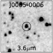
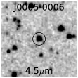
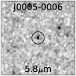
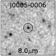
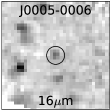
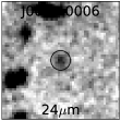
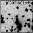
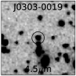
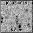
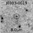
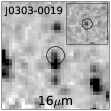
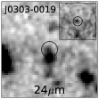
Figure 1.— Spitzer images of the two quasars previously undetected in the longer Spitzer bands: J0005$-$0006 (top) and J0303$-$0019 (bottom). All panels show an area of 1′$\times$1′. The circle indicating the quasar position has a diameter of 10″. For J0303$-$0019 the inset at the two longest wavelengths show a 40″$\times$40″ subimage around the quasar position after subtracting the bright confusing source (see text). This confusing source is also visible in the IRAC frames where it is well separated from the quasar itself.

II.3. Photometry in z and y bands

We also compiled z-band and y-band photometry for the majority of the sample (see Table II.1). For most of the quasars, the z-band photometry is taken from SDSS or from the discovery papers, which sometimes presented deeper observations.

The y-band photometry was mainly provided by Pan-STARRS (Kaiser et al., 2010), complemented by data from UKIDSS (Lawrence et al., 2007). For objects where the NIR photometry (see below) was taken from UKIDSS, we also used the y-band flux from this survey, for consistency. In most cases where y-band data exist from both surveys they agree within the combined errors.

II.4. NIR photometry

An important source of photometry in the $J$, $H$, and/or $K$ bands were the discovery papers (or follow-up work on those). In the majority of cases, magnitudes were given in a Vega-based system and were obtained with a multitude of instruments across our sample. We here consistently use the values given in Hewett et al. (2006) to convert all the Vega-based magnitudes into the AB system. The NIR photometry from the literature was complemented by photometry from UKIDSS for a sizable fraction of our sample. For additional nine objects we obtained $J$-band photometry using Omega2000 at the 3.5m telescope of the Calar Alto observatory. For the data reduction and photometry we followed standard procedures. Magnitudes and the corresponding references are reported in Table II.1.

Table 3Spitzer IRS photometry at 16 $\mu$m.

Source	flux
	$\mu$Jy
(1)	(2)
J0005$-$0006	24$\pm$	8
J0303$-$0019	59$\pm$	20
J0353+0104	225$\pm$	30
J0818+1722	666$\pm$	63
J0842+1218	610$\pm$	66
J1137+3549	306$\pm$	31
J1250+3130	696$\pm$	31
J1411+1217	120$\pm$	26
J1427+3312	128$\pm$	15
J2315$-$0023	107$\pm$	20

II.5. Spitzer

Mid-infrared imaging from Spitzer exists for all Herschel targets, with the exception of J2054$-$0005. These data consist of observations at 3.6, 4.5, 5.8, and 8.0 $\mu$m with IRAC (Fazio et al., 2004) as well as at 24 $\mu$m with MIPS (Rieke et al., 2004). A small number of objects was also observed at 16 $\mu$m with the peak-up array of IRS (Houck et al., 2004).

The Spitzer data were processed in a standard manner using procedures within the MOPEX software package provided by the Spitzer Science Center (SSC). The resulting maps from IRAC and MIPS are presented in the Appendix in Figure A.1. Aperture photometry on the final images was performed in IDL. In most cases we used apertures with a radius of 3.6, 5.4, and 7 arcseconds in IRAC, IRS, and MIPS, respectively. For some objects the aperture size was reduced to avoid contamination from nearby objects. Appropriate aperture corrections were taken from the respective instrument handbooks (also available from the SSC website).

Errors on the photometry were determined by measuring the fluxes in 500 apertures (with sizes identical to the science target aperture) which were randomly placed on source-free regions of the background, avoiding area of low coverage. The distribution of these 500 fluxes was fit by a Gaussian. The sigma of this Gaussian was taken as the 1$\sigma$ uncertainty on the photometry. The measured fluxes and uncertainties are presented in Table II.6.1 for IRAC and MIPS. The additional IRS photometry for a small subset of objects is presented in Table 3. We note that some of the Spitzer data have been published previously (e.g., Hines et al., 2006; Jiang et al., 2006, 2010) and in these cases our photometry is consistent with the earlier results.

For a few objects, direct aperture photometry (even with smaller apertures) was difficult to obtain due to severe blending with neighboring sources. In such cases we used the point source extraction tool APEX in the MOPEX software package to subtract the confusing source from the science image. We then performed aperture photometry as described above on the residual image (i.e. where the confusing source has been removed) for consistency with the rest of the sample.

II.6. Herschel

II.6.1 PACS

We observed all objects at 100 $\mu$m (green channel) and 160 $\mu$m (red channel) with PACS (Poglitsch et al., 2010). We employed the mini-scan map observing template with parameters as recommended in the corresponding Astronomical Observation Template release note, which includes a combination of two scans with different scan directions. For each scan direction, five repetitions were executed. The total on-source integration time was $\sim$ 900 s for each object.

Table 4Millimeter photometry from the literature.

Source	$F_{250\,{\rm GHz}}$		reference
	mJy
(1)	(2)		(3)
J0002+2550	$<2.6$		5
J0005$-$0006	$<1.4$		4
J0203+0012	1.85$\pm$	0.46	1
J0231$-$0728	$<3.5$		3
J0303$-$0019	$<1.5$		4
J0338+0021	3.7$\pm$	0.3	2
J0353+0104	$<1.4$		4
J0756+4104	5.5$\pm$	0.5	3
J0818+1722	1.19$\pm$	0.38	4
J0836+0054	$<2.9$		3
J0840+5624	3.20$\pm$	0.64	5
J0841+2905	$<1.3$		4
J0842+1218	$<1.7$		4
J0913+5919	$<2.8$		3
J0927+2001	4.98$\pm$	0.75	4
J1030+0524	$<3.4$		5
J1044$-$0125	1.82$\pm$	0.43	4
J1048+4637	3.0$\pm$	0.4	6
J1137+3549	$<3.4$		5
J1148+5251	5.0$\pm$	0.6	6
J1204$-$0021	$<1.8$		2
J1208+0010	$<3.1$		3
J1250+3130	$<2.7$		5
J1306+0356	$<3.1$		3
J1335+3533	2.34$\pm$	0.50	5
J1411+1217	$<1.9$		5
J1427+3312	$<2.0$		4
J1436+5007	$<3.4$		5
J1602+4228	$<1.6$		4
J1623+3112	$<2.4$		5
J1630+4012	$<1.8$		4
J2054$-$0005	2.38$\pm$	0.53	4
J2315$-$0023	$<1.8$		4

The data were processed within the Herschel Interactive Processing Environment (HIPE, Ott 2010), version 10. We followed standard procedures for deep field data reduction, including source masking and high-pass filtering. The two scan directions were processed individually and later combined into a final map. The half-width of the high-pass filter was set to 12 and 16 samples in green and red, respectively. Considering the scan speed of 20 ″/s used for our observations and the effective sampling of 10 Hz of the bolometer pixels, this corresponds to a total high-pass filter window of 50″ (green) and 66″ (red) on sky. Source masking was performed via circular masks of typically 6 to 8″ size (or larger if needed given the source structure). The mask was created by hand through visual inspection of the mosaicked maps. For this purpose we first created a map (with both scan directions combined) without source masking. On this map we masked all visible sources and source structures that could lead to artifacts during high-pass filtering. This proved to be more reliable than a strict sigma cut, as it also allowed the masking of fairly faint features which could potentially influence the measured fluxes of our faint science targets, if located nearby. The data were then reprocessed including the source mask. Only in a few cases it was necessary to improve the mask using this new map. The frames contributing to the final map were selected based on the scan speed and we adopted a limit of $\pm$ 5 ″/s around the nominal scan speed of 20 ″/s. During map projection, the pixel fraction parameter (e.g., Fruchter & Hook, 2002) was set to 0.6 to take advantage of the moderate redundancy in our data provided by the repetition factor of five. We show images around the QSOs position at 100 $\mu$m and 160 $\mu$m in the Appendix (Figure A.1).

Table 5Source photometry.

Source	redshift	$F_{3.6\mu{\rm m}}$		$F_{4.5\mu{\rm m}}$		$F_{5.8\mu{\rm m}}$		$F_{8.0\mu{\rm m}}$		$F_{24\mu{\rm m}}$		$F_{100\mu{\rm m}}$		$F_{160\mu{\rm m}}$		$F_{250\mu{\rm m}}$		$F_{350\mu{\rm m}}$		$F_{500\mu{\rm m}}$
		$\mu$Jy		$\mu$Jy		$\mu$Jy		$\mu$Jy		$\mu$Jy		mJy		mJy		mJy		mJy		mJy
(1)	(2)	(3)		(4)		(5)		(6)		(7)		(8)		(9)		(10)		(11)		(12)
J0002+2550	5.80	119$\pm$	2	152$\pm$	2	123$\pm$	6	150$\pm$	7	747$\pm$	31	3.5$\pm$	1.0	8.6$\pm$	1.8	$<13.2$		$<13.8$		$<15.6$
J0005$-$0006	5.85	33$\pm$	1	43$\pm$	1	31$\pm$	5	22$\pm$	3	52$\pm$	17	$<2.4$		$<4.8$		$<14.4$		$<15.6$		$<16.5$
J0017$-$1000	5.01	171$\pm$	2	145$\pm$	2	171$\pm$	6	251$\pm$	6	1580$\pm$	33	3.8$\pm$	0.5	7.3$\pm$	0.9	$<13.5$		$<13.5$		$<15.5$
J0054$-$0109	5.09	70$\pm$	1	59$\pm$	1	69$\pm$	5	85$\pm$	5	376$\pm$	43	4.3$\pm$	1.4	$<6.6$		$<14.4$		$<13.8$		$<16.2$
J0133+0106	5.30	60$\pm$	2	86$\pm$	1	65$\pm$	5	79$\pm$	6	255$\pm$	49	$<3.9$		$<6.6$		$<14.4$		$<14.7$		$<17.4$
J0203+0012	5.72	80$\pm$	2	89$\pm$	2	104$\pm$	5	105$\pm$	7	680$\pm$	49	$<3.0$		$<6.0$		$<15.6$		$<13.5$		$<18.0$
J0231$-$0728	5.41	128$\pm$	2	178$\pm$	1	138$\pm$	6	144$\pm$	7	433$\pm$	42	$<4.2$		$<5.7$		$<13.5$		$<13.8$		$<16.2$
J0303$-$0019	6.08	29$\pm$	1	38$\pm$	1	22$\pm$	5	34$\pm$	6	72$\pm$	24	$<3.0$		$<5.4$		$<14.1$		$<12.6$		$<15.3$
J0338+0021	5.00	80$\pm$	2	70$\pm$	2	81$\pm$	7	156$\pm$	9	1186$\pm$	51	11.4$\pm$	1.1	22.3$\pm$	2.5	19.6$\pm$	5.9	18.5$\pm$	6.2	12.6$\pm$	6.5
J0353+0104	6.07	61$\pm$	2	71$\pm$	2	56$\pm$	9	76$\pm$	14	368$\pm$	92	$<3.6$		$<6.3$		$<18.9$		$<21.9$		$<24.6$
J0731+4459	5.01	165$\pm$	3	133$\pm$	3	138$\pm$	7	226$\pm$	8	1585$\pm$	45	$<3.6$		$<5.7$		$<15.0$		$<14.4$		$<18.3$
J0756+4104	5.09	62$\pm$	2	62$\pm$	2	71$\pm$	5	120$\pm$	5	698$\pm$	45	6.4$\pm$	1.1	10.2$\pm$	2.2	11.4$\pm$	5.3	19.0$\pm$	4.8	19.9$\pm$	5.0
J0818+1722	6.00	166$\pm$	1	202$\pm$	2	166$\pm$	8	212$\pm$	9	1004$\pm$	36	$<4.2$		$<6.3$		$<14.7$		$<13.8$		$<15.3$
J0833+2726	5.02	67$\pm$	2	53$\pm$	2	55$\pm$	7	76$\pm$	6	429$\pm$	48	$<4.2$		$<6.3$		$<13.2$		$<13.8$		$<16.8$
J0836+0054	5.81	258$\pm$	2	418$\pm$	1	282$\pm$	5	303$\pm$	6	929$\pm$	52	6.3$\pm$	1.3	$<6.3$		$<16.2$		$<16.2$		$<16.2$
J0840+5624	5.84	56$\pm$	1	69$\pm$	1	58$\pm$	5	63$\pm$	5	440$\pm$	37	$<3.3$		$<6.9$		$<15.3$		$<13.5$		$<15.3$
J0841+2905	5.96	46$\pm$	2	53$\pm$	2	49$\pm$	7	78$\pm$	8	543$\pm$	39	$<3.6$		$<6.0$		$<14.1$		$<15.3$		$<16.8$
J0842+1218	6.06	81$\pm$	1	98$\pm$	2	88$\pm$	8	128$\pm$	10	1292$\pm$	75	5.9$\pm$	1.3	16.1$\pm$	2.3	$<19.8$		$<29.1$		$<24.6$
J0846+0800	5.04	74$\pm$	2	61$\pm$	2	66$\pm$	6	108$\pm$	9	510$\pm$	56	$<3.6$		$<6.9$		$<16.2$		$<16.2$		$<19.2$
J0901+6942	5.47	61$\pm$	1	79$\pm$	1	71$\pm$	4	89$\pm$	5	532$\pm$	35	$<3.6$		$<5.4$		$<15.6$		$<13.8$		$<17.4$
J0902+0851	5.22	64$\pm$	1	84$\pm$	1	66$\pm$	4	85$\pm$	5	399$\pm$	22	$<3.3$		$<5.4$		$<14.1$		$<15.6$		$<17.4$
J0913+5919	5.11	35$\pm$	1	39$\pm$	1	37$\pm$	1	53$\pm$	2	280$\pm$	32	$<3.0$		$<6.6$		$<14.4$		$<13.8$		$<15.9$
J0915+4924	5.20	87$\pm$	2	108$\pm$	2	89$\pm$	6	115$\pm$	7	583$\pm$	53	$<3.0$		$<7.5$		$<14.1$		$<13.8$		$<15.6$
J0922+2653	5.06	57$\pm$	2	51$\pm$	2	49$\pm$	6	82$\pm$	7	388$\pm$	27	$<3.3$		$<6.9$		$<14.7$		$<15.3$		$<18.0$
J0927+2001	5.77	47$\pm$	2	50$\pm$	2	43$\pm$	7	74$\pm$	7	639$\pm$	47	$<3.6$		7.3$\pm$	2.3	13.1$\pm$	5.3	15.3$\pm$	5.0	19.5$\pm$	5.8
J0957+0610	5.19	115$\pm$	2	142$\pm$	1	136$\pm$	8	247$\pm$	9	1148$\pm$	51	5.0$\pm$	1.3	11.3$\pm$	2.1	14.0$\pm$	5.0	$<15.3$		$<16.8$
J1013+4240	5.06	61$\pm$	2	53$\pm$	2	51$\pm$	6	70$\pm$	6	302$\pm$	36	$<3.3$		$<5.4$		$<14.4$		$<12.9$		$<13.8$
J1030+0524	6.31	74$\pm$	3	90$\pm$	2	52$\pm$	7	84$\pm$	9	425$\pm$	60	$<3.6$		$<6.6$		$<14.7$		$<14.7$		$<17.7$
J1044$-$0125	5.78	106$\pm$	2	125$\pm$	2	109$\pm$	7	190$\pm$	8	1436$\pm$	45	6.3$\pm$	1.2	7.7$\pm$	1.8	$<15.3$		$<12.6$		$<16.5$
J1048+4637	6.23	110$\pm$	1	122$\pm$	2	95$\pm$	6	127$\pm$	7	818$\pm$	35	2.8$\pm$	0.5	5.7$\pm$	1.0	$<14.4$		$<14.1$		$<18.6$
J1119+3452	5.02	76$\pm$	1	63$\pm$	1	69$\pm$	5	125$\pm$	5	578$\pm$	40	$<3.3$		$<6.9$		$<14.7$		$<13.2$		$<17.4$
J1132+1209	5.17	145$\pm$	2	175$\pm$	2	171$\pm$	7	281$\pm$	8	1176$\pm$	49	7.0$\pm$	1.0	$<7.2$		$<12.9$		$<12.9$		$<15.6$
J1137+3549	6.01	84$\pm$	2	99$\pm$	2	90$\pm$	9	89$\pm$	10	579$\pm$	34	$<3.9$		$<6.3$		$<13.8$		$<12.6$		$<17.1$
J1146+4037	5.01	184$\pm$	2	157$\pm$	2	172$\pm$	6	217$\pm$	6	779$\pm$	33	$<3.0$		$<6.3$		$<14.7$		$<16.8$		$<17.7$
J1148+5251	6.43	136$\pm$	2	143$\pm$	2	145$\pm$	7	208$\pm$	8	1349$\pm$	49	4.1$\pm$	0.9	7.4$\pm$	1.9	21.0$\pm$	5.3	21.8$\pm$	4.9	12.4$\pm$	5.7
J1148+5253	5.70	11$\pm$	1	13$\pm$	1	$<15$		$<15$		$<105$		$<3.3$		$<5.4$		$<15.0$		$<14.7$		$<15.9$
J1154+1341	5.08	77$\pm$	1	64$\pm$	1	68$\pm$	4	107$\pm$	5	470$\pm$	47	$<3.3$		$<7.5$		$<12.6$		$<13.2$		$<19.8$
J1202+3235	5.31	125$\pm$	2	147$\pm$	2	150$\pm$	6	233$\pm$	7	1609$\pm$	49	8.3$\pm$	1.1	16.3$\pm$	2.2	18.4$\pm$	5.2	24.6$\pm$	5.2	13.7$\pm$	5.6
J1204$-$0021	5.03	110$\pm$	1	109$\pm$	1	122$\pm$	5	209$\pm$	7	1312$\pm$	28	11.6$\pm$	1.2	14.7$\pm$	2.3	30.8$\pm$	4.6	40.0$\pm$	4.6	29.1$\pm$	5.8
J1208+0010	5.27	23$\pm$	1	30$\pm$	1	23$\pm$	4	23$\pm$	4	$<78$		$<3.0$		$<6.0$		$<12.9$		$<12.0$		$<15.3$
J1221+4445	5.19	97$\pm$	1	127$\pm$	1	106$\pm$	5	163$\pm$	5	689$\pm$	37	$<3.3$		$<6.0$		$<13.2$		$<13.5$		$<18.3$
J1242+5213	5.05	114$\pm$	1	92$\pm$	1	92$\pm$	5	84$\pm$	6	291$\pm$	31	$<3.0$		$<4.8$		$<14.1$		$<14.1$		$<16.2$
J1250+3130	6.13	84$\pm$	1	108$\pm$	1	92$\pm$	7	140$\pm$	7	1366$\pm$	25	$<3.6$		$<5.4$		$<14.1$		$<14.4$		$<20.7$
J1306+0356	6.02	73$\pm$	3	81$\pm$	3	54$\pm$	7	57$\pm$	7	365$\pm$	55	$<3.3$		$<5.4$		$<13.5$		$<13.2$		$<18.3$
J1334+1220	5.14	87$\pm$	1	94$\pm$	1	93$\pm$	4	165$\pm$	5	1089$\pm$	56	5.4$\pm$	1.0	6.5$\pm$	1.7	$<14.4$		$<12.6$		$<15.6$
J1335+3533	5.90	66$\pm$	1	70$\pm$	1	55$\pm$	4	58$\pm$	5	456$\pm$	19	$<3.3$		$<6.6$		$<13.5$		$<14.1$		$<18.6$
J1337+4155	5.03	95$\pm$	1	68$\pm$	1	66$\pm$	5	99$\pm$	5	564$\pm$	45	$<3.6$		5.4$\pm$	1.7	$<13.5$		$<14.1$		$<18.6$
J1340+3926	5.07	112$\pm$	1	107$\pm$	1	109$\pm$	4	176$\pm$	5	1267$\pm$	36	6.1$\pm$	1.1	7.5$\pm$	1.9	$<13.8$		$<13.2$		$<15.9$
J1340+2813	5.34	129$\pm$	1	169$\pm$	1	171$\pm$	6	250$\pm$	6	1485$\pm$	43	9.8$\pm$	1.2	16.2$\pm$	2.2	21.8$\pm$	5.0	22.4$\pm$	4.9	$<16.5$
J1341+4611	5.01	68$\pm$	1	53$\pm$	1	55$\pm$	4	81$\pm$	4	492$\pm$	44	$<4.2$		$<5.4$		$<14.4$		$<12.9$		$<17.1$
J1411+1217	5.93	87$\pm$	2	137$\pm$	2	88$\pm$	6	97$\pm$	7	168$\pm$	52	$<3.6$		$<6.3$		$<14.1$		$<15.0$		$<17.1$
J1423+1303	5.08	118$\pm$	1	104$\pm$	1	104$\pm$	5	167$\pm$	6	947$\pm$	23	$<3.0$		$<7.2$		$<15.0$		$<14.7$		$<16.2$
J1427+3312	6.12	58$\pm$	1	71$\pm$	2	75$\pm$	6	62$\pm$	7	411$\pm$	58	$<3.6$		$<5.4$		$<16.2$		$<15.0$		$<16.8$
J1436+5007	5.83	44$\pm$	1	49$\pm$	1	35$\pm$	5	59$\pm$	12	365$\pm$	35	$<3.3$		$<7.2$		$<12.6$		$<13.8$		$<15.3$
J1443+3623	5.29	146$\pm$	2	191$\pm$	2	204$\pm$	6	396$\pm$	6	3029$\pm$	36	9.4$\pm$	1.0	12.6$\pm$	1.9	15.3$\pm$	4.6	$<12.9$		$<18.9$
J1510+5148	5.11	124$\pm$	2	113$\pm$	1	109$\pm$	4	137$\pm$	5	770$\pm$	34	$<3.6$		$<5.7$		$<14.7$		$<13.5$		$<15.6$
J1524+0816	5.08	39$\pm$	2	45$\pm$	2	27$\pm$	6	61$\pm$	11	343$\pm$	43	$<3.6$		$<6.3$		$<14.1$		$<14.1$		$<18.9$
J1602+4228	6.07	135$\pm$	2	157$\pm$	2	126$\pm$	5	159$\pm$	6	840$\pm$	35	7.7$\pm$	1.1	13.8$\pm$	2.4	10.9$\pm$	4.5	10.5$\pm$	4.6	$<17.7$
J1614+4640	5.31	138$\pm$	1	184$\pm$	1	161$\pm$	5	228$\pm$	5	998$\pm$	51	5.1$\pm$	1.4	$<7.2$		$<15.3$		$<15.6$		$<21.0$
J1623+3112	6.25	74$\pm$	2	97$\pm$	2	71$\pm$	5	89$\pm$	6	623$\pm$	34	2.4$\pm$	0.6	$<3.6$		$<15.6$		$<14.7$		$<16.8$
J1626+2751	5.30	325$\pm$	1	395$\pm$	1	367$\pm$	6	498$\pm$	6	2672$\pm$	56	8.5$\pm$	1.3	13.1$\pm$	2.0	19.9$\pm$	4.6	28.4$\pm$	5.7	19.9$\pm$	6.2
J1626+2858	5.02	81$\pm$	2	70$\pm$	2	72$\pm$	6	110$\pm$	6	717$\pm$	44	2.3$\pm$	0.6	$<3.0$		$<15.9$		$<15.3$		$<15.9$
J1630+4012	6.07	37$\pm$	2	43$\pm$	2	26$\pm$	5	37$\pm$	6	148$\pm$	21	$<4.2$		$<7.2$		$<14.4$		$<15.0$		$<17.4$
J1659+2709	5.32	135$\pm$	3	163$\pm$	2	163$\pm$	6	234$\pm$	8	1858$\pm$	48	6.8$\pm$	1.2	7.2$\pm$	2.1	$<17.9$		$<19.8$		$<20.1$
J2054$-$0005	6.04	$\cdots$		$\cdots$		$\cdots$		$\cdots$		$\cdots$		3.1$\pm$	1.0	10.5$\pm$	2.0	15.2$\pm$	5.4	12.0$\pm$	4.9	$<19.5$
J2119+1029	5.18	53$\pm$	1	65$\pm$	3	63$\pm$	5	88$\pm$	5	586$\pm$	24	2.0$\pm$	0.5	$<3.3$		$<14.4$		$<13.6$		$<17.1$
J2228$-$0757	5.14	93$\pm$	2	120$\pm$	2	90$\pm$	7	88$\pm$	7	250$\pm$	22	$<1.5$		$<3.9$		$<13.8$		$<14.4$		$<15.0$
J2245+0024	5.17	23$\pm$	2	29$\pm$	1	27$\pm$	5	36$\pm$	5	96$\pm$	24	$<3.9$		$<6.6$		$<13.8$		$<15.0$		$<15.6$
J2315$-$0023	6.12	33$\pm$	1	40$\pm$	1	32$\pm$	5	37$\pm$	4	158$\pm$	22	4.9$\pm$	1.2	$<6.3$		$<14.4$		$<14.4$		$<18.3$

Note. — (1) source name; (2) observed 250 GHz flux in mJy. Errors are 1$\sigma$, upper limits are 3$\sigma$; (3) references for column (2)

References. — (1) Wang et al. 2011; (2) Carilli et al. 2001; (3) Petric et al. 2003; (4) Wang et al. 2008b; (5) Wang et al. 2007; (6) Bertoldi et al. 2003

Note. — Col.: (1) Source name; (2) Redshift; (3)-(7) Photometry in the Spitzer bands in $\mu$mJy. (8)-(12) Photometry in the Herschel bands in mJy.

Source fluxes or upper limits were determined via aperture photometry in IDL. We used apertures of 6″ and 9″ radius in green and red, respectively. A residual sky was measured in a sky annulus between 20″ and 25″ (green) or 24″ and 28″ (red). Appropriate aperture corrections were determined from the encircled energy fraction of unresolved sources provided as part of the calibration data.

The uncertainties of the Herschel maps was determined in a similar fashion as for the Spitzer data: For a given map we performed aperture photometry at 500 random positions across the map. The placement of the apertures was limited to regions in the scan map with at least 75 % of the coverage compared to the science target. The aperture radius was fixed to the value used for the quasar photometry. The distribution of these 500 flux measurements was then fitted with a Gaussian, the sigma of which we take as the 1$\sigma$ uncertainty on the photometry (e.g., Lutz et al., 2011; Popesso et al., 2012). For a few objects, slight changes in the photometry scripts resulted in revised error estimates compared to Leipski et al. (2013).

We have also re-observed six sources with unusual MIR ($\sim$4–15 $\mu$m rest frame) SEDs during Herschel’s second open time cycle. These targets were undetected in our standard Herschel observations and we selected sources with unusually small 100 $\mu$m/24 $\mu$m flux limits for deeper observations. The observational layout and data reduction procedure was similar to that of the standard observations. We executed additional three visits for each source with the same parameters as before, essentially quadrupling the on-source integration time. The new fluxes and deeper flux limits are included and marked in Table II.6.1 where we report the full Herschel photometry results. Note that the error estimates in Table II.6.1 do not include the $\sim$5% uncertainty on the absolute flux calibration (Balog et al., 2013).

II.6.2 SPIRE

The SPIRE (Griffin et al., 2010) instrument on board Herschel was used to observe all quasars in our sample at 250, 350, and 500 $\mu$m. The observations were carried out in small scan map mode with five repetitions for each objects, totaling $\sim$ 190 s on-source integration time per source. This observational set-up ensured that our maps are dominated by confusion noise which is on the order of $6-7$ mJy beam^-1 in the SPIRE photometric bands (Nguyen et al., 2010).

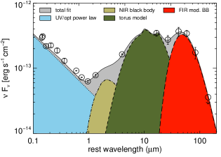
Figure 2.— Schematic representation of the components used for SED fitting. As an example we use the observed photometry of the $z=5.03$ QSO J1204$-$0021.

Table 6Results of the SED fitting.

Source	$L_{\rm UV/opt}$		$L_{\rm MIR}$		$T_{\rm FIR}$		$L_{\rm FIR}$		SFR
	($10^{46}$ erg s-1)		($10^{46}$ erg s-1)		(K)		($10^{13}$ $L_{\odot}$)		($10^{3}M_{\odot}$ yr-1)
(1)	(2)		(3)		(3)		(5)		(6)
J0002+2550	10.1$\pm$	0.3	10.7$\pm$	0.8	47		$<$0.9		$<$1.5
J0017$-$1000	10.2$\pm$	0.2	10.5$\pm$	0.3	47		$<$0.7		$<$1.2
J0338+0021	6.2$\pm$	0.2	19.8$\pm$	1.1	51$\pm$	6	1.2$\pm$	0.5	2.1$\pm$	0.6
J0756+4104	5.7$\pm$	0.2	11.2$\pm$	0.4	40$\pm$	2	1.0$\pm$	0.2	1.7$\pm$	0.3
J0842+1218	9.5$\pm$	0.4	23.6$\pm$	1.6	47		$<$1.3		$<$2.2
J0927+2001	5.8$\pm$	0.2	$<$9.9		49$\pm$	2	1.1$\pm$	0.2	1.9$\pm$	0.3
J0957+0610	10.4$\pm$	0.2	13.4$\pm$	0.7	47		$<$0.7		$<$1.2
J1044$-$0125	9.6$\pm$	0.3	18.4$\pm$	1.3	53$\pm$	3	1.1$\pm$	0.2	1.9$\pm$	0.3
J1048+4637	11.0$\pm$	0.2	11.8$\pm$	0.6	47		$<$1.3		$<$2.2
J1148+5251	14.5$\pm$	0.2	18.2$\pm$	0.8	60$\pm$	3	3.5$\pm$	0.5	6.0$\pm$	0.6
J1202+3235	16.9$\pm$	0.3	20.9$\pm$	0.7	47		$<$0.9		$<$1.5
J1204$-$0021	9.4$\pm$	0.2	18.1$\pm$	0.7	51$\pm$	5	2.4$\pm$	0.3	4.1$\pm$	0.5
J1334+1220	7.8$\pm$	0.2	11.5$\pm$	0.6	47		$<$0.8		$<$1.3
J1340+3926	8.8$\pm$	0.2	20.3$\pm$	0.8	47		$<$0.7		$<$1.2
J1340+2813	9.8$\pm$	0.3	12.3$\pm$	0.5	47		$<$0.8		$<$1.3
J1443+3623	13.1$\pm$	0.4	27.2$\pm$	1.0	47		$<$0.8		$<$1.3
J1602+4228	9.1$\pm$	0.4	21.0$\pm$	1.8	47		$<$0.6		$<$1.0
J1626+2751	23.2$\pm$	0.4	22.9$\pm$	1.5	47		1.9$\pm$	0.3	3.2$\pm$	0.5
J1659+2709	15.6$\pm$	0.2	17.3$\pm$	1.3	47		$<$1.3		$<$2.2

Data reduction was performed in HIPE (version 10) following standard procedures as recommended by the SPIRE instrument team. The SPIRE final maps are shown alongside the Spitzer and PACS images in the Appendix (Figure A.1). The HIPE build-in source extractor ’sourceExtractorSussextractor’ (Savage & Oliver, 2007) was used to locate sources and determine source fluxes, including a pixelisation correction. Instead of using global average confusion noise limits (Nguyen et al., 2010), we estimated these uncertainties specifically for our target fields in the following manner (see also, Elbaz et al., 2011; Pascale et al., 2011): First, the source extractor was run over the full calibrated maps. An artificial source image including all the sources found by the source extractor was created and subtracted from the observed map. On this “residual map” we determined the pixel-to-pixel rms in a box with a size of 8 times the FWHM (FWHM size: 18.2″, 24.9″, and 36.3″ for default map pixel sizes of 6, 10, and 14″ at 250, 350, and 500 $\mu$m, respectively), centered on the nominal position of the QSO. The size of this box was chosen large enough to allow an appropriate sampling of the surroundings of the source, but small enough to avoid including the lower coverage areas at the edges of the map even for the longest wavelengths. In addition, the number of pixels per FWHM is approximately constant for the three wavelengths in the final maps ($2.5-3.0$ px/FWHM) which translates into a similar number of pixels used for determining the rms in the background box. The resulting estimates for the noise (limited by confusion) are comparable to the global average values given in Nguyen et al. (2010), but have a tendency to be slightly lower. Detections from the source extraction located within less than half the FWHM from the nominal target position were tentatively considered to belong to the quasar. The measured source flux was then compared to the estimated confusion noise in the map. We also checked for confusion with nearby FIR bright sources using our multi-wavelength data to avoid mis-identifications. The final source photometry is presented in Table II.6.1. Similar to PACS, the SPIRE errors in Table II.6.1 do not include the $\sim$4% uncertainty on the absolute flux calibration (Bendo et al., 2013).

We note that a number of SPIRE flux measurements in Table II.6.1 are nominally below the estimated 3$\sigma$ value of the noise. In such cases, the images reveal a clear excess of flux at the position of the quasar and comparison with other wavelengths (e.g. Spitzer/24 $\mu$m or PACS) shows no clear indication for possible confusion issues. The use of positional priors can reduce the effect of confusion noise by 20-30 % (Roseboom et al., 2010), and our data set provides accurate (relative and absolute) positional information as well as information on the SEDs of the quasar and potential confusing sources in the field. Therefore, we here include these flux measurements in our study, although they have to be treated with caution. Similarly, fluxes at 500 $\mu$m should be considered tentative because at this wavelength the beam is large ($\sim$ 36 ″ FWHM), the confusion noise is high, and the significance of the detections is often low.

II.6.3 Millimeter regime

In total, 33 objects of our Herschel sample have published observations in the millimeter regime from the ground, typically at 250 GHz (see Tab. 4). The 11 millimeter detections among those have been presented in detail in Leipski et al. (2013), but are also included here. The remaining 22 objects are undetected at millimeter wavelengths. Among those 22, five sources (J0002+2550, J0842+1218, J1048+4637, J1204$-$0021, J1602+4228) have Herschel detections in two or more bands, while the rest is also undetected with Herschel. A number of the millimeter observed objects have also been targeted in the sub-millimeter from the ground (Priddey et al., 2003, 2008; Robson et al., 2004; Wang et al., 2008a, 2010; Beelen et al., 2006) and recently with ALMA (Wang et al., 2013).

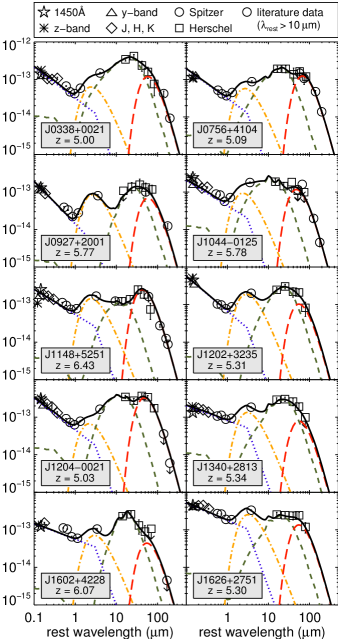
Figure 3.— The SEDs of the 10 quasars detected in at least four Herschel bands. The plots shows $\nu F_{\nu}$ in units of erg s^-1 cm^-2 over the rest frame wavelength. The colored lines indicate the results of a multi-component SED fit as described in Section IV.1. They consist of a power-law (blue dotted), a black body of T $\sim$ 1200 K (yellow dash-dotted), a torus model (green dashed), and a modified black body of $\sim$47 K (see Table 6; red long dashed). The black solid line shows the total fit as the sum of the individual components.

III. Detection rates

Most of the objects in our sample had previously only been observed in the optical or NIR. These data sample the rest frame UV/optical regime and typically provide spatial resolution of $\sim$1″ or higher. Therefore caution has to be exercised when matching such objects with data in the FIR where often only (much) lower spatial resolution is achievable and sources faint in the optical but bright in the FIR could be mistaken as a counterpart. For a reliable source matching, the multi-wavelength nature of our data set provided a powerful tool for determining the exact position of the quasar in the Herschel bands. In particular the Spitzer 24 $\mu$m images were very valuable in this regard. They provide spatial resolution bridging the gap between the optical/NIR and FIR observations and strong detections for most quasars in our sample. In many cases we can identify several sources per field that are visible both at Spitzer and at Herschel wavelengths and the exact location of the quasar in the Herschel maps can be determined from the relative positional information. With this procedure we can robustly identify faint Herschel detections with the quasars as well as avoid mis-identifications due to nearby objects. During this exercise we observe absolute spatial offsets between Spitzer and Herschel of typically $\lesssim$ 2″, in line with expectations from the absolute pointing accuracies (Sánchez-Portal et al. 2014, submitted).

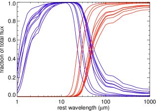
Figure 4.— For the ten objects where the FIR component could be well constrained due to additional millimeter data (see Figure 3) we here show its relative contributions (red) compared to the presumably AGN-heated dust (NIR black body plus torus model; blue) as a function of wavelength. For these FIR-bright sources, the FIR component dominates the total infrared emission at $\lambda_{\rm rest}$ $\gtrsim$ 50 $\mu$m.

In almost all cases we detect the observed quasars in the available Spitzer bands at high significance (see Table II.6.1). One exception is J1148+5253 which is neither detected with IRAC at 5.8 and 8 $\mu$m nor with MIPS at 24 $\mu$m. However, this object is almost 3 magnitudes fainter in z-band than the majority of the sample. The only other exception is J1208+0010 which we do not detect in MIPS at 24 $\mu$m. Our detections include those quasars which have previously been dubbed ’dust-free’ (Jiang et al., 2010). In our analysis we see both sources (J0005$-$0006 and J0303$-$0019) at all Spitzer wavelengths (Figure 1). While J0005$-$0006 is fairly isolated and can be identified readily, the other object (J0303$-$0019) suffers from blending issues with a nearby source. In the higher spatial resolution IRAC observations the two objects can be well separated, but with IRS and MIPS the blending becomes severe. In these cases we subtracted the confusing source as described in Section II.5. In both bands we see significant residual flux at the position of the quasar. The new detections of these two objects, however, do not change the basic conclusion of Jiang et al. (2010) that these quasars are clearly deficient of hot dust compared to the majority of the sample.

With PACS we only see 22 (100 $\mu$m) and 19 (160 $\mu$m) objects at greater than 3$\sigma$ significance in our standard observations. In a number of objects the exactly determined position (see above) was crucial to avoid misidentifications. With SPIRE the detection rate is even lower and we identify only 10 objects which are bright enough in the observed FIR/sub-mm range to be detected systematically (i.e., at 250 $\mu$m as well as at 350 $\mu$m) above the confusion noise.

The additional deep PACS observations for six objects undetected by our standard Herschel program result in two quasars detected in both bands and three sources detected only at 100 $\mu$m at faint flux levels. One source remained undetected with an upper limit more than a factor of 2 below our standard limit.

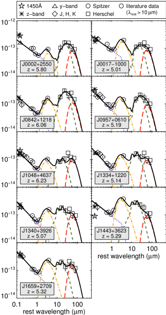
Figure 5.— The SEDs of the 9 quasars detected in 2 or 3 Herschel bands shown in $\nu F_{\nu}$ in units of erg s^-1 cm^-2 over the rest frame wavelength. Color coding of the fitted components as in Figure 3.

IV. Analysis and dicussion

IV.1. SED fitting

Ten quasars in our sample have been detected in at least four of the five Herschel bands (Table II.6.1). In combination with their Spitzer fluxes and using supplemental NIR data, the combined photometry provides SEDs covering the rest frame wavelengths from 0.1 to $\sim$80 $\mu$m. To assess some basic physical properties of these objects, we perform SED fitting, following the approach presented in Leipski et al. (2013). To summarize briefly, the SEDs are fitted with four components: a power-law in the UV/optical mainly representing emission from the accretion disk, a black body from hot ($\sim$1200 K) dust, a torus model from the library of Hönig & Kishimoto (2010), and an additional cool dust component in the form of a modified black body ($\beta$ = 1.6). We illustrate this approach and the arrangement of the fitted components schematically in Figure 2.

In Leipski et al. (2013) we already presented five of the ten FIR detected quasars, all of which had millimeter detections. The five additional sources presented here do not have mm detections and sub-millimeter/millimeter upper limits exist only for two of the five newly presented objects. In the case of J1204$-$0021 (Carilli et al., 2001; Priddey et al., 2003) those data points can be used to provide additional constraints on the temperature which is consequently treated as a free parameter. For J1602+4228 (Wang et al., 2008b) the 250 GHz upper limit does not strongly constrain the temperature of the fitted FIR component and we fix $T_{\rm FIR}$ to a value of 47 K for this object (Beelen et al., 2006; Wang et al., 2007; Leipski et al., 2013). For the remaining three objects, the temperature of the FIR component was also fixed to 47 K. Due to the lack of mm data which would help to anchor the Rayleigh-Jeans tail of the FIR component, the fits would otherwise predict artificially increased dust temperatures (Leipski et al., 2013).

Figure 6.— The ratio of the AGN-dominated dust-to-accretion disk emission decreases with UV/optical luminosity. The data are taken from Table 6 and correspond to the UV/optical luminosity between 0.1 $\mu$m and 1 $\mu$m and the AGN-heated dust emission between 1 $\mu$m and 1000 $\mu$m (NIR bump plus torus, but excluding the additional FIR component). All wavelengths refer to the rest frame of the source. Errorbars correspond to $\pm$3 $\sigma$.

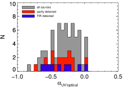
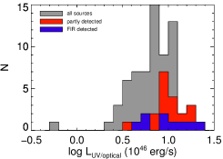
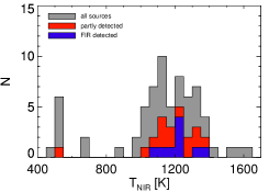
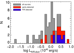
Figure 7.— Parameter value distributions from the UV/optical plus NIR fits (Section IV.2). Top, left: UV/optical power-law index $\alpha$ ($F_{\nu}$ $\propto$ ${\nu}^{\alpha}$). Top, right: luminosity of the power-law component integrated between 0.1 $\mu$m and 1 $\mu$m. Bottom, left: temperature of the hot dust component. Bottom, right: luminosity of the hot dust component integrated between 1 $\mu$m and 3 $\mu$m. The Herschel detected objects (blue and red histograms) are preferentially found at the high-luminosity end in $L_{\rm UV/opt}$ as well as in $L_{\rm NIR}$ but show no particular trends in $\alpha$ or $T_{\rm NIR}$.

The rest frame UV/optical and infrared SEDs of these ten objects can be fitted well with a combination of these four components. The best fitting model combinations are shown in Figure 3 and Table 6 summarizes some basic properties determined from the fitting. Using these fits we also determine the relative contributions of the different components to the total infrared SED. For this we combine the dust component in the NIR and the torus model, both of which are likely to be powered by the AGN. We compare this AGN related emission to the additional FIR component and show their relative contributions to the total infrared emission as a function of wavelength in Figure 4. We see that in the presence of luminous FIR emission ($L_{\rm FIR}$ $\sim$ 10¹³ $L_{\odot}$), this component dominates the total infrared SED at rest frame wavelengths above $\sim$50 $\mu$m for all ten objects. This means that in such cases of strong FIR/sub-millimeter emission, rest frame wavelengths $\gtrsim$50 $\mu$m isolate the additional FIR component without the need for full SED fits (at least in our modeling approach). The possible heating source for the additional FIR component (AGN versus star formation) is further discussed in section IV.4.

We also extend a similar SED fitting approach to objects with fewer Herschel detections. In cases where two PACS detections are available (9 sources), these data provide sufficient constraints for the torus model, while the upper limits in the SPIRE bands (and in the millimeter where avilable, se Tab. 4) limit the contribution of the additional FIR component (fixed to a temperature of 47 K). These fits are presented in Figure 5 and some basic properties derived from the fitted components are presented in Table 6. From this table we use the UV/optical luminosity and the AGN-dominated dust luminosity to show that the ratio of the AGN-dominated dust-to-accretion disk emission decreases with increasing UV/optical luminosity (Figure 6). This behavior may reflect the increase of the dust sublimation radius for more luminous UV/optical continuum emitters (e.g., Barvainis, 1987) which, under the assumption of a constant scale height, is often explained in terms of a decreasing dust covering factor with increasing luminosity in the context of the so-called receding torus model (Lawrence, 1991).

The measured FIR fluxes for our 10 FIR detected objects fall only moderatly above the 3$\sigma$ confusion noise limit (Table II.6.1). Thus, the photometric upper limits for the 9 FIR non-detections (i.e. only detected in PACS) yield upper limits on $L_{\rm FIR}$ that do not differ significantly from the detection on an individual basis (Table 6). Further constraints on the average FIR properties of the PACS-only sources are provided by a stacking analysis as presented in Section IV.4.

IV.2. The SEDs at $\lambda_{\rm rest}$ $<$ 4 $\mu$m

For two thirds of the sample, the upper limits in the Herschel observations do not provide strong constraints to MIR or FIR components to allow full SED fitting. We therefore chose to limit the fitting to rest frame wavelengths corresponding to the MIPS 24 $\mu$m band ($\sim$3-4 $\mu$m rest frame) and shorter where the majority of the sources is well detected. For these data we fit a combination of a power-law in the UV/optical and a hot black body in the NIR. To minimize the influence from emission lines (e.g., Ly$\alpha$, H$\alpha$) and the small blue bump on the fitted power-law slope, we limit the data points to Spitzer bands at $\lambda_{\rm obs}$ $\geq$ 5.8 $\mu$m and only using the y-band photometry in the rest frame UV. In those cases where no y-band photometry is available (5 objects), we use the z-band instead. For selected sources the UV part of the rest frame SEDs was excluded from the fitting to avoid broad absorption line features (e.g. J0203+0012, J1427+3312). The resulting fits are shown in Figure 14.

We derive UV/optical luminosities for the quasars by integrating the fitted power-law between 0.1 $\mu$m and 1 $\mu$m. Similarly, for the hot dust component, the NIR dust luminosity is provided by integrating the fitted black body between 1 $\mu$m and 3 $\mu$m. The fitted values for $\alpha_{\rm UV/opt}$ ($F_{\nu}$ $\propto$ ${\nu}^{\alpha}$) and $T_{\rm NIR}$, as well as the integrated luminosities for the two components, are given in Table 7 and their distributions are shown in Figure 7.

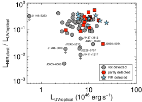
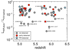
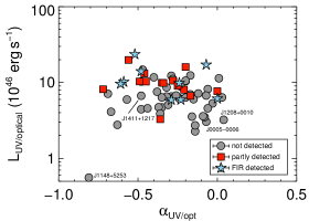
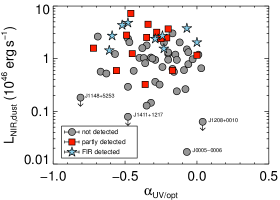
Figure 8.— Results from the UV/optical plus NIR fits (Section IV.2). Error bars in the legend indicate typical errors in the respective panels. Top, left: UV/optical to NIR luminosity ratio as a function of UV/optical luminosity. The luminosity ratio does not show any obvious trend over the UV/optical luminosity range we sample, indicating that both luminosity measures are correlated. There is also no trend with redshift seen (top right) which could indicate either redshift evolution or possible artifacts from sampling SEDs at different redshifts with fairly broad filters. Both panels show a group of objects which have low luminosity ratio compared to the majority of sources. Bottom row: Both luminosity measures do not show any obvious trends with the UV/optical power-law index $\alpha$ ($F_{\nu}$ $\propto$ ${\nu}^{\alpha}$).

In the distributions in Figure 7 we also indicate the Herschel FIR detected objects (blue) and the partly detected objects (red; see Section IV.4 for the definition of these samples). While no specific trends can be identified for $\alpha_{\rm UV/opt}$ or $T_{\rm NIR}$, Figure 7 reveals that Herschel detections are preferentially found at the high end of the UV/optical luminosity distribution (see also, Netzer et al., 2013). This is even more pronounced for the NIR luminosity $L_{\rm NIR,dust}$ (Figure 7, bottom right).

We also find a group of objects which have very low temperatures of the hot dust component in our fitting approach (Figure 7, bottom left). We caution that the actual temperature values provided by our fitting are not well defined in these cases because the data only poorly constrain $T_{\rm NIR}$. Nevertheless, the SEDs clearly demonstrate that these objects have a dearth of very hot dust compared to their UV/optical luminosity, and compared to the remainder of the sample. The reduced contributions from hot dust to the SEDs is also reflected in their lower values for $L_{\rm NIR,dust}$. In the individual SED plots (Figure 14) these objects can be identified from their shallow rise in flux between the observed bands at 8 $\mu$m and 24 $\mu$m (Figure 9). Often, the observed IRAC 8 $\mu$m data point is still dominated by the power law and not by the onset of the hot dust emission as traced by the MIPS 24 $\mu$m photometry. In such cases the 24 $\mu$m photometry itself only very moderately exceeds the predictions from the power law.

Altogether we find that $\sim$12–16% of the sample have NIR to UV/optical properties that are quite different from the rest of the sample. Such sources have been found in similar proportions in other samples (e.g., Jiang et al., 2010; Hao et al., 2011; Mor & Netzer, 2012). Jun & Im (2013) show that the fraction of dust-poor quasars increases with optical luminosity and redshift, and our numbers are consistent with their trends. These authors suggest that the dust-poor phase is a transient phenomenon during the evolution of the quasar (e.g., Jiang et al., 2010), rather than a distinct population of quasars with low covering factors (e.g., Hao et al., 2011).

The rest of our objects has $L_{\rm NIR,dust}$/$L_{\rm UV/opt}$ between $\sim$0.08 $-$ 0.5 and we see no trends in this ratio with redshift or $L_{\rm UV/opt}$ (Figure 8). The latter implies that the luminosities in the UV/optical and NIR are well correlated for most objects (see also, Mor & Netzer, 2012). This is not surprising considering that the accretion disk emission, here traced by the UV/optical luminosity, is expected to be the primary heating source of the hot dust. Neither $L_{\rm UV/opt}$ nor $L_{\rm NIR}$ show any trend with $\alpha_{\rm UV/opt}$ (Figure 8). Similarly, $T_{\rm NIR}$ shows no obvious trends with $\alpha_{\rm UV/opt}$ or $L_{\rm UV/opt}$, while $\alpha_{\rm UV/opt}$ is uncorrelated with redshift.

Table 7UV/optical and NIR properties.

Source	$\alpha$		$L_{\rm UV/opt}$		${\nu}L_{\nu,{\rm 5100\AA}}$		$T_{\rm NIR}$	$L_{\rm NIR}$		${\nu}L_{\nu,6.7\mu{\rm m}}$		EW Ly$\alpha$	reference	EW H$\alpha$	Fν,cont
			($10^{46}$erg s-1)		($10^{46}$erg s-1)		(K)	($10^{46}$erg s-1)		($10^{46}$erg s-1)		Å		Å
(1)	(2)		(3)		(4)		(5)	(6)		(7)		(8)	(9)	(10)	(11)
J0002+2550	-0.	45	10.	29	3.	23	1076	1.	25	3.	78	60.0	6	336	12.	1
J0005$-$0006	-0.	07	3.	04	0.	70	500	0.	02	$<$0.	76	81.5	10	455	3.	2
J0017$-$1000	-0.	48	10.	29	3.	28	1110	2.	41	4.	41	55.2	11	$\cdots$	$\cdots$
J0054$-$0109	-0.	17	6.	67	1.	68	1127	0.	60	1.	93	12.3	11	$\cdots$	$\cdots$
J0133+0106	-0.	48	4.	44	1.	42	1036	0.	29	$<$1.	66	$\cdots$	$\cdots$	689	6.	2
J0203+0012	-0.	20	10.	40	2.	68	1079	1.	23	$<$3.	24	35.9	10	-21	9.	0
J0231$-$0728	-0.	29	12.	25	3.	40	500	0.	36	$<$2.	49	83.8	11	500	13.	3
J0303$-$0019	-0.	08	3.	50	0.	81	1600	0.	26	$<$1.	16	139.4	10	714	2.	5
J0338+0021	-0.	29	5.	90	1.	64	1205	2.	38	5.	43	42.5	11	$\cdots$	$\cdots$
J0353+0104	-0.	67	4.	11	1.	49	1042	0.	57	$<$2.	95	$\cdots$	10	307	5.	9
J0731+4459	-0.	17	12.	39	3.	12	1184	3.	02	$<$4.	33	57.4	11	$\cdots$	$\cdots$
J0756+4104	-0.	23	5.	92	1.	57	1251	1.	55	3.	31	30.5	11	$\cdots$	$\cdots$
J0818+1722	-0.	47	14.	70	4.	66	1156	2.	05	$<$5.	23	10.0	8	309	16.	6
J0833+2726	-0.	63	2.	76	0.	98	1039	0.	52	$<$2.	00	$\cdots$	$\cdots$	$\cdots$	$\cdots$
J0836+0054	-0.	56	19.	84	6.	67	500	0.	59	5.	58	70.0	2	724	26.	9
J0840+5624	-0.	06	8.	19	1.	88	1040	0.	78	$<$3.	91	$\cdots$	$\cdots$	281	5.	7
J0841+2905	-0.	35	4.	71	1.	37	1344	1.	79	$<$3.	45	58.0	9	166	4.	7
J0842+1218	-0.	35	9.	93	2.	89	1042	2.	53	7.	18	$\cdots$	$\cdots$	238	8.	4
J0846+0800	-0.	15	6.	02	1.	50	1291	1.	19	$<$2.	14	28.4	11	$\cdots$	$\cdots$
J0901+6942	-0.	29	6.	54	1.	82	1115	0.	95	$<$2.	72	55.0	5	301	6.	5
J0902+0851	-0.	44	4.	57	1.	42	1093	0.	59	$<$1.	95	109.6	11	598	6.	5
J0913+5919	-0.	16	3.	55	0.	89	1210	0.	56	$<$1.	42	110.9	11	$\cdots$	$\cdots$
J0915+4924	0.	01	11.	36	2.	46	1203	1.	19	$<$2.	35	78.1	11	462	8.	8
J0922+2653	-0.	03	5.	31	1.	19	1316	0.	97	$<$1.	76	57.8	11	$\cdots$	$\cdots$
J0927+2001	0.	00	6.	13	1.	33	1321	2.	04	$<$3.	47	$\cdots$	$\cdots$	141	4.	5
J0957+0610	-0.	28	10.	60	2.	91	1360	3.	17	4.	32	51.4	11	$\cdots$	$\cdots$
J1013+4240	0.	03	6.	36	1.	35	1256	0.	66	$<$1.	50	41.5	11	$\cdots$	$\cdots$
J1030+0524	-0.	12	7.	17	1.	73	1550	2.	04	$<$3.	54	70.0	2	670	6.	3
J1044$-$0125	-0.	34	9.	88	2.	85	1329	4.	49	7.	00	26.0	1	213	10.	7
J1048+4637	-0.	28	11.	11	3.	05	1311	2.	67	4.	21	40.0	4	275	10.	3
J1119+3452	-0.	07	6.	73	1.	57	1339	1.	50	$<$2.	22	33.8	11	$\cdots$	$\cdots$
J1132+1209	-0.	49	10.	32	3.	33	1315	2.	79	4.	94	40.8	11	$\cdots$	$\cdots$
J1137+3549	-0.	20	10.	58	2.	72	994	0.	96	$<$3.	79	$\cdots$	$\cdots$	202	8.	7
J1146+4037	-0.	40	11.	69	3.	52	1098	1.	04	$<$2.	58	58.6	11	$\cdots$	$\cdots$
J1148+5251	-0.	48	14.	04	4.	48	1362	4.	80	7.	01	25.0	4	33	14.	0
J1148+5253	-0.	81	0.	56	0.	22	1100	$<$0.	18	$<$1.	17	$\cdots$	$\cdots$	29	1.	3
J1154+1341	-0.	37	4.	73	1.	39	1273	1.	03	$<$2.	01	51.9	11	$\cdots$	$\cdots$
J1202+3235	-0.	07	17.	16	3.	98	1238	3.	78	6.	84	16.1	11	141	13.	6
J1204$-$0021	-0.	24	9.	83	2.	63	1224	2.	72	5.	93	53.9	11	$\cdots$	$\cdots$
J1208+0010	0.	04	3.	23	0.	68	869	$<$0.	06	$<$0.	72	$\cdots$	$\cdots$	592	2.	3
J1221+4445	-0.	38	7.	55	2.	25	1292	1.	59	$<$2.	69	105.8	11	$\cdots$	$\cdots$
J1242+5213	-0.	32	6.	53	1.	85	500	0.	15	$<$1.	41	49.3	11	$\cdots$	$\cdots$
J1250+3130	-0.	69	7.	10	2.	61	1043	2.	63	$<$5.	99	$\cdots$	$\cdots$	334	8.	8
J1306+0356	-0.	17	6.	97	1.	75	692	0.	64	$<$2.	75	60.0	2	399	6.	3
J1334+1220	-0.	21	8.	04	2.	10	1250	2.	48	4.	20	49.7	11	$\cdots$	$\cdots$
J1335+3533	-0.	24	6.	15	1.	64	537	0.	69	$<$2.	94	-5.0	8	212	6.	1
J1337+4155	-0.	00	7.	70	1.	68	1220	1.	16	$<$2.	26	78.8	11	$\cdots$	$\cdots$
J1340+3926	-0.	25	9.	02	2.	42	1177	2.	41	4.	68	59.6	11	$\cdots$	$\cdots$
J1340+2813	-0.	59	10.	18	3.	50	1159	2.	72	7.	06	69.3	11	241	14.	7
J1341+4611	-0.	36	3.	89	1.	13	1142	0.	82	$<$2.	17	110.7	11	$\cdots$	$\cdots$
J1411+1217	-0.	48	6.	69	2.	14	500	$<$0.	08	$<$1.	81	100.0	6	783	8.	7
J1423+1303	-0.	23	8.	83	2.	33	1235	2.	01	$<$3.	01	48.4	11	$\cdots$	$\cdots$
J1427+3312	-0.	26	6.	73	1.	82	694	0.	32	$<$3.	20	$\cdots$	7	123	6.	5
J1436+5007	-0.	06	4.	57	1.	05	1407	1.	33	$<$2.	52	$\cdots$	$\cdots$	316	4.	0
J1443+3623	-0.	46	13.	16	4.	15	1253	7.	22	10.	43	28.3	11	221	17.	1
J1510+5148	-0.	32	8.	61	2.	44	1056	1.	05	$<$2.	87	72.4	11	$\cdots$	$\cdots$
J1524+0816	-0.	14	2.	27	0.	56	1351	0.	95	$<$1.	70	$\cdots$	$\cdots$	$\cdots$	$\cdots$
J1602+4228	-0.	61	9.	60	3.	35	1067	1.	44	6.	53	$\cdots$	$\cdots$	292	13.	1
J1614+4640	-0.	72	8.	15	3.	04	1147	1.	58	4.	22	61.7	11	424	14.	8
J1623+3112	-0.	57	5.	97	2.	03	1063	1.	22	3.	43	150.0	6	499	7.	3
J1626+2751	-0.	52	23.	54	7.	74	1117	4.	34	9.	33	45.6	11	268	34.	4
J1626+2858	-0.	20	6.	33	1.	63	1171	1.	32	2.	23	18.9	11	$\cdots$	$\cdots$
J1630+4012	-0.	09	3.	59	0.	84	1505	0.	61	$<$1.	97	70.0	4	539	3.	1
J1659+2709	-0.	20	16.	00	4.	13	1157	3.	67	6.	92	30.3	11	181	14.	7
J2054$-$0005	$\cdots$		$\cdots$		$\cdots$		$\cdots$	$\cdots$		$\cdots$		17.0	10	$\cdots$	$\cdots$
J2119+1029	-0.	31	5.	07	1.	43	1130	1.	01	2.	00	$\cdots$	$\cdots$	$\cdots$	$\cdots$
J2228$-$0757	-0.	35	6.	36	1.	85	500	0.	13	$<$1.	04	115.7	11	$\cdots$	$\cdots$
J2245+0024	-0.	14	2.	72	0.	67	1371	0.	24	$<$0.	84	115.0	3	$\cdots$	$\cdots$
J2315$-$0023	-0.	36	3.	29	0.	96	1145	0.	32	2.	26	126.8	10	332	3.	3

By including the PACS 100 $\mu$m band, we extend the analysis to slightly longer infrared wavelengths and determine the flux at a rest frame wavelength of 6.7 $\mu$m through interpolation of the observed photometry at 24 $\mu$m and 100 $\mu$m using a power law in $\nu F_{\nu}$. In combination with the monochromatic luminosity at 5100Å (rest frame) as provided by our UV/optical power-law fits, we can study the monochromatic ratio of MIR-to-optical emission as a function of (monochromatic) optical luminosity (Figure 10). Under the assumption that the infrared-to-optical luminosity ratio is a proxy of the dust covering factor in (type 1) AGN, a plot as in Figure 10 has been used by Maiolino et al. (2007) to identify a trend where the dust covering factor decreases with increasing optical luminosity. Such a general behavior of the dust covering factor (or obscured fraction of AGN) has been detected for many different samples and using various techniques (e.g. Treister et al., 2008; Hasinger, 2008; Lusso et al., 2013, and references therein) and is also seen in our sample for the Herschel detected objects (Figure 6). However, the question whether the covering factor also changes with redshift remains controversial, with claims for (Treister & Urry, 2006; Hasinger, 2008) and against (Ueda et al., 2003; Lusso et al., 2013) significant redshift evolution.

In this context, our high-redshift QSOs show a systematic, albeit very moderate offset in the MIR-to-optical luminosity ratio with respect to $2.0\lesssim z\lesssim 3.5$ QSOs (Figure 10). Much of the observed offset is currently driven by the Herschel detections where the 6.7 $\mu$m flux is determined as the interpolation between two significantly detected data points at $\lambda_{\rm obs}$ of 24 $\mu$m and 100 $\mu$m. However, about 60% of the $z>5$ objects have only upper limits on the MIR-to-optical ratio, mostly due to non-detections in the 100 $\mu$m band. While in Figure 10 these objects currently populate the same area as the Herschel 100 $\mu$m detected objects (colored symbols), their effect on the observed trends remain unclear. This is in particular emphasized when considering the wide range of intrinsic SED shapes that may be present among the Herschel non-detected sources (see Section IV.4), which could potentially result in a wider range of luminosity ratios than seen currently for the Herschel detected objects. For example, if the $z>5$ objects intrinsically showed the same spread in the MIR-to-optical ratio as the $2.0\lesssim z\lesssim 3.5$ sample (almost 1 dex in Figure 10) then the resulting distribution would be roughly consistent with the observed trends at lower redshift.

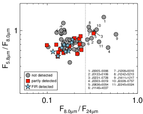
Figure 9.— Observed flux ratios for three Spitzer bands demonstrating the selection of sources deficient in hot dust emission on observational grounds alone. Most of the QSOs in our sample that fall to the right of the dotted line (which indicates $F_{8\mu{\rm m}}/F_{24\mu{\rm m}}=0.25$) also have low $L_{\rm NIR,dust}/L_{\rm UV/opt}$ $<$ 0.05 (Figure 8 and Table 7).

On the other hand Figure 10 reveals that the data points and upper limits with the lowest MIR-to-optical ratio among our sample in Figure 10 almost exclusively belong to the group of objects where the SEDs indicate a dearth of hot dust. These objects may be of different nature or reside in a different evolutionary state (e.g., Jiang et al., 2010; Hao et al., 2011; Mor & Trakhtenbrot, 2011; Jun & Im, 2013) and possibly cannot be directly compared with the other QSOs from either sample.

IV.3. H$\alpha$ equivalent widths

H$\alpha$ is one of the most prominent emission lines in the UV/optical spectra of common quasars (e.g., Vanden Berk et al., 2001). For our high-redshift objects ($z>5$), this emission line is redshifted into the observed mid infrared, largely precluding direct spectroscopic observations with current facilities. However, we can use our high signal-to-noise Spitzer photometry to estimate H$\alpha$ fluxes. For redshifts greater than $z\sim 5.2$, the influence of this line can be seen in the individual SEDs (Figure 14) where H$\alpha$ emission boosts the flux in the 4.5 $\mu$m IRAC band compared to a power-law continuum (e.g., J0840+5624). At lower redshift ($z<5.2$), H$\alpha$ falls onto the flanks of the filter transmission or largely into the small gap between the 3.6 $\mu$m and 4.5 $\mu$m IRAC filter. This makes it difficult to extract reliable emission-line flux estimates from the observed photometry. At $z\gtrsim 5.2$ and up to our maximum redshift ($z=6.42$), the H$\alpha$ emission line is fully covered by the filter transmission window and peaks within the plateau region of the 4.5 $\mu$m filter.

For the purpose of estimating H$\alpha$ line fluxes we fit the SEDs slightly differently as compared to Section IV.2 or as shown in Figure 14. Instead of considering the full UV/optical continuum for a power-law fit we now limit the fit to the neighboring photometric points in order to isolate the local continuum. This means that for an H$\alpha$ line falling into the 4.5 $\mu$m band we fit the power law to the 3.6 $\mu$m and 5.8 $\mu$m bands only. From the offset of the measured flux in the 4.5 $\mu$m filter compared to the local estimate of the power-law continuum we then calculate the H$\alpha$ emission-line flux and equivalent width (EW). We show the distribution of the estimated H$\alpha$ EWs in Figure 11 and the derived values are also provided in Table 7. When comparing our high-$z$ results to spectroscopic H$\alpha$ EWs from low redshift ($z\lesssim 0.4$) SDSS quasars (Shen et al., 2011), we see that the two distributions are quite similar in width and shape. This similarity between low and high-redshift quasars indicates a lack of redshift evolution in the H$\alpha$ EWs, which agrees with similar results for rest-frame UV emission lines (Iwamuro et al., 2004; Juarez et al., 2009; De Rosa et al., 2011).

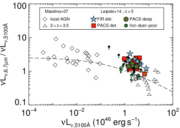
Figure 10.— The ratio of the MIR luminosity at 6.7 $\mu$m and the optical luminosity at 5100Å (all in the rest frame) as a proxy for the dust covering factor plotted over the optical luminosity. Open symbols as well as the dashed trend line are taken from Maiolino et al. (2007). Filled symbols refer to all 68 high-redshift QSOs from this work for which the relevant luminosities could be determined. The dark green circles show the five quasars for which the deep re-observations resulted in a 100 $\mu$m detection. Data points marked with bright green dots represent objects with a dearth of hot dust as determined from Figure 4. Many of the sources with 3$\sigma$ upper limits in the plotted luminosity ratio populate the same area as (and are concealed by) the Herschel detections (i.e., by the filled colored symbols).

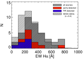
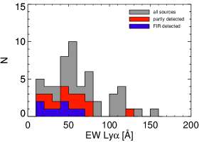
Figure 11.— Left: Distribution of H$\alpha$ equivalent widths in the sample (grey filled area, estimated as outlined in Section IV.3. As a hashed region we show the histogram of the H$\alpha$ equivalent widths of $\sim$4800 SDSS quasars taken from Shen et al. (2011). Right: Distribution of Ly$\alpha$ equivalent widths for our high-$z$ sample, taken from the literature.

From Figure 11 (left) we can also see that the Herschel detected objects, and in particular the FIR detected objects, have preferentially low H$\alpha$ EWs. This trend is also seen in the Ly$\alpha$ EWs (Figure 11, top right) as taken from the literature (Table 7). Such a prevalence of FIR bright objects among sources with low Ly$\alpha$ EW has previously been indicated for mm-detected high-redshift quasars (e.g., Omont et al., 1996; Bertoldi et al., 2003; Wang et al., 2008b). Wang et al. (2008b) speculated that in these objects a special dust geometry that only affects the broad emission line clouds (and not the continuum) could in principle lead to such an effect. Because the impact of dust obscuration on H$\alpha$ would be much smaller than for Ly$\alpha$, the persisting trend of Herschel FIR detected objects to be found at low H$\alpha$ EW values questions such a scenario. However, while the effects of obscuration are indeed reduced for H$\alpha$ compared to Ly$\alpha$, they can still be non-negligible. A more definite answer requires higher precision direct spectroscopic measurements, preferably of (rest frame) NIR emission lines, to further reduce the effect of possible dust obscuration.

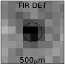
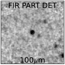
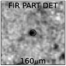
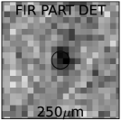
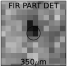
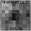
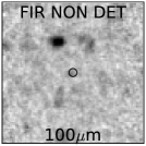
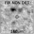
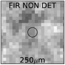
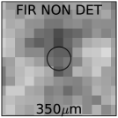
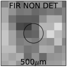
Figure 12.— Stacked images in the Herschel bands for the three subsamples outlined in section IV.4. The images have a size of 2′on a side, the circle indicating the central position has a diameter corresponding to the FWHM at the respective wavelength.

IV.4. Stacking

Due to the large number of Herschel non-detections in our sample, we have used a stacking approach to study the average infrared properties of the high-redshift quasars. For this purpose we divided the full sample into three subsamples:

1. 10 FIR-detected objects with detections in at least three Herschel bands (160 $\mu$m, 250 $\mu$m, and 350 $\mu$m).

2. 14 partly (Herschel) detected objects with significant PACS 100 $\mu$m and/or 160 $\mu$m flux. We refer to this subsample also as the PACS-only objects.

3. 33 (Herschel) non-detections.

The remaining objects have been excluded from the stacking analysis on various grounds: 10 objects suffer from confusion with nearby FIR bright sources which would influence the stacked fluxes. The science targets on these images are not detected with Herschel individually. Two additional sources, J1148+5253 and J2245+0024, have been excluded because they are significantly fainter in the optical/UV than the rest of the sample. Both are also Herschel non-detections.

The stacking was performed in flux in the observed frame and the resulting mean SEDs were shifted into rest frame using the median redshift in the respective subsamples. In the y-band and in the Spitzer bands (where virtually all objects in all three subsamples are individually detected) we used the observed photometry as input. For Herschel the final images where stacked pixel by pixel centered on the position of the quasar. Photometry on the resulting stacks was performed as described for the individual images (Sections II.6.1 and II.6.2). The mean stacks in the Herschel bands for the three subsamples are presented in Figure 12. To estimate the variation present within these subsamples we followed a bootstrapping approach. For a given subsample we randomly selected as many objects as there are members in that subsample, allowing for replacements, created a new stack and performed photometry. This was done for 1000 random combinations of objects in each subsample. The centroid of the distribution of these 1000 individual stacked photometry values was then taken as the final average flux of the subsample. We use the standard deviation of this distribution, which can be considered a measure for the variety of intrinsic SED shapes present in the subsample, as the uncertainty on the average flux. The overall significance of the final stacked mean value in the Herschel bands was determined as follows: we stacked the images at random positions on the background, following a similar procedure as for the quasar positions. If the mean value of the source stack distribution is larger than three times the mean value of the background stack distribution we consider the stacked quasar signal to be significant.

In Figure 13 (left) we compare the average SEDs of the FIR-detected objects (blue SED) with that of the partly detected objects (red SED). The SEDs are very similar in absolute scaling and spectral shape up to and including the observed 100 $\mu$m band ($\sim$15 $\mu$m rest frame). At longer wavelengths, however, the SEDs are very different. In the $\nu F_{\nu}$ representation of Figure 13 (left), the PACS-only objects show a steep drop above $\sim$20 $\mu$m rest frame while the FIR detected objects display an additional component towards the FIR. This behavior is emphasized in Figure 13 (right) where we show the average SEDs normalized by the shape of the mean SED of the partly-detected objects.

The partly Herschel detected sources (red SED in Figure 13) are optically luminous AGN with powerful NIR and MIR emission, but without exceptional FIR brightness, at least on average. The shape of the SED is very similar to the average SDSS quasar SED and beyond $\sim$20 $\mu$m broadly resembles the shape of typical torus models (e.g., Schartmann et al., 2008; Nenkova et al., 2008; Hönig & Kishimoto, 2010; Stalevski et al., 2012). In these cases the AGN is likely contributing significantly or even dominantly to the FIR emission (Netzer et al., 2007; Lutz et al., 2008; Wang et al., 2008b). However, the upper limits in the SPIRE bands are not very stringent and would still be consistent with a FIR component of $\sim$10¹² $L_{\odot}$ (assuming a modified black body of T = 47 K and $\beta$ = 1.6). Therefore, it cannot be ruled out that star formation contributes FIR emission on levels of a few tens to a few hundred solar masses per year as found for other high-redshift QSOs (Wang et al., 2008b; Venemans et al., 2012; Willott et al., 2013; Netzer et al., 2013). We note that for some combinations of objects the bootstrapping indeed reveals significant detections in the SPIRE bands, indicating that some sources in this subsample were just below the individual detection limit. In the global mean, however, the partly Herschel detected subsample only reaches $\sim$2$\sigma$ significance in the stacked values at 250 $\mu$m and 350 $\mu$m.

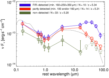
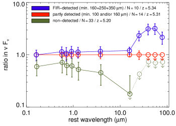
Figure 13.— Left: Average SEDs for three subsamples as defined in Section IV.4. The dashed line is the SDSS quasar template (Richards et al., 2006). Right: The average SEDs divided by the SED of the partly Herschel detected sample (red). This emphasizes the differences in the SED shape between the three samples.

The comparison of the average SEDs of the two Herschel-detected subsamples emphasizes that AGN with strong emission in the UV/optical (from the accretion disk) throughout the NIR and MIR (from AGN-powered hot and warm dust) do not necessarily show considerable FIR emission as well (both panels in Figure 13; see also Dai et al. 2012). The fact that some optical and MIR luminous QSOs show strong FIR emission and others do not may indicate that star formation is the dominant driver for the additional FIR component observed in the Herschel FIR detected QSOs. This is consistent with the results of Lutz et al. (2008) who show that for a sample of millimeter bright QSOs at $z\sim 2$ the PAH and FIR luminosities correlate, which also supports star formation as the source of the FIR emission in powerful FIR bright AGN (these objects have optical luminosities comparable to our sources). For some high-redshift millimeter bright QSOs it has been shown that the potentially star-formation dominated FIR continuum and line emission (e.g. of [CII]) is concentrated in the innermost kiloparsecs (e.g., Walter et al., 2009; Wang et al., 2013). At the highest luminosities, the close proximity to the AGN may thus still lead to significant contributions from the AGN to the FIR emission (e.g., Dai et al. 2012, see also Valiante et al. 2011). For such sources future observation at high resolution may provide additional clues on the relative AGN-to-SF contributions to the dust heating from the spatial distribution of the cold dust emission.

The average SED of the Herschel non-detections (green SEDs in Figure 13) differs from the SEDs of the Herschel detected sources in several aspects. Even at 100 $\mu$m (observed) we only find a barely significant detection in the maximum flux case (as provided by the bootstraping), and non-detections for most realizations as well as for the mean of this subsample. No detection was obtained for any combination of objects at longer wavelengths. A significant difference between the average SED of this subsample and those of objects with individual Herschel detections is that the UV/optical and NIR/MIR fluxes are systematically smaller, and accordingly also the luminosities because the median redshifts of the three subsamples are very similar. This has already been indicated by the UV/optical and NIR luminosity distributions of the full sample (Figure 7) where the Herschel detected sources are found to be clustered at the high luminosity end. This flux difference in the mean increases towards longer wavelengths (factor of 1.4 at $\sim$0.5 $\mu$m rest frame and factor of 5 at $\sim$15 $\mu$m rest frame; see also Blain et al. 2013). From Figure 13 it appears that on average the shape of the infrared SED is changing for fainter QSOs, even though taking into account the full errors bars shown in that figure could reduce the trend seen for the mean. This behavior is in principle supported by the individual objects that have deeper re-observations. These were drawn from the Herschel non-detected subsample, and by selection correspond to sources with high observed 24 $\mu$m fluxes in this sample (above the average for all but one of the six sources). Individually they also show a decline in $\nu F_{\nu}$ between 24 $\mu$m and 100 $\mu$m, but shallower than the average SED.

The flux levels of the Herschel/PACS 100 $\mu$m detections for these deeper data show that they were not far below the sensitivity limit of our standard observations. Even though a number of objects apparently only barely avoided detection in our standard data, the final average SED of the Herschel non-detections (which includes these objects just below the detection limit) shows steeper 24 $\mu$m to 100 $\mu$m slopes and remains Herschel PACS non-detected in most cases. This supports the idea that the Herschel non-detected subsample includes objects with a wide range of intrinsic SED shapes and that many of the sources in this sub sample are much fainter in the 100 $\mu$m band than our detection limit.

We note that four objects in this Herschel non-detected subsample have individual millimeter detections (Bertoldi et al., 2003; Wang et al., 2007, 2011) and were discussed in Leipski et al. (2013). Considering the shape of the SED in the (AGN dominated) MIR, we can speculate that the cold dust emission responsible for the millimeter flux (typically $\sim$$2-3$ mJy at 1.2 mm observed) is probably powered by star formation in these cases (see also Wang et al., 2008b; Leipski et al., 2013).

Figure 14.— The SEDs of the 52 quasars with only one (6 sources) or no (45 sources) Herschel detection, or where no SED fitting could be performed (J2054$-$0005) due to missing Spitzer data, shown in $\nu F_{\nu}$ in units of erg s^-1 cm^-2 over the rest frame wavelength. Photometry symbols as in Figures 3 and 5. The solid line shows a combined power-law (dotted line) and black body (dashed line) fit as outlined in section IV.2.

Figure 14.— continued

V. Summary and Conclusions

We studied the spectral energy distributions of 69 QSOs at redshift $z>5$, covering rest frame wavelengths from 0.1 to $\sim$80 $\mu$m. For this purpose we presented new Herschel observations in five bands between 100 $\mu$m and 500 $\mu$m which we combined with mostly unpublished Spitzer data, also in five bands (3.6 $\mu$m to 24 $\mu$m). Photometry from the literature and large area surveys in the optical and near infrared completed the wavelength coverage. Our main results are:

1. The detection rate with Spitzer is very high, with only two objects lacking detections in the longest bands. The detection rate decreases towards the (observed) far infrared where Herschel detected $\sim$30% in PACS (100/160 $\mu$m) and $\sim$15% in SPIRE (250/350 $\mu$m).

2. All objects with a sufficient number of Herschel detections (typically in at least two bands) were subject to multi-component SED fitting using the full wavelength range. All of them required a hot dust component (T $\sim$ 1200 K) in addition to an AGN torus model to fit the near and mid-infrared emission. The objects with rest frame FIR detections (i.e. in the SPIRE bands) also needed an additional cold (T $\sim$ 50 K) component with $L_{\rm FIR}$ on the order of 10¹³ $L_{\odot}$.

3. At shorter wavelengths ($\lambda_{\rm obs}$ $\leq$ 24 $\mu$m, $\lambda_{\rm rest}$ $\lesssim$ 4 $\mu$m, ), the high detection rate facilitated the study of the UV/optical and NIR properties of most objects in our sample. For this purpose we fitted a power-law in the rest frame UV/optical in combination with a black body in the NIR to the observed photometry. The distribution of the resulting parameters shows that the Herschel detected objects are preferentially found at the high luminosity end of our sample (for $L_{\rm UV/opt}$ and in particular for $L_{\rm NIR}$). No such trends are seen for the UV/optical power-law index or the temperature of the NIR black body. $L_{\rm UV/opt}$ and $L_{\rm NIR}$ are correlated and their luminosity ratio does not show significant trends with optical luminosity or redshift. We identify a group of objects corresponding to $\sim$15% of the full sample that shows low $L_{\rm NIR}/L_{\rm UV/opt}$ ratios. Such objects seem to be deficient in hot dust compared to most of the other quasars.

4. We determined the monochromatic luminosities at a rest frame wavelength of 6.7 $\mu$m (from the observed photometry in the 24 $\mu$m and 100 $\mu$m bands) and at 5100Å (from the UV/optical power-law fit). The resulting MIR-to-optical luminosity ratio tends to be higher at $z>5$ than for redshift $2-3$ QSOs of comparable optical luminosity, at least for the objects with Herschel detections at 100 $\mu$m. However, about 60% of the $z>5$ sample have only upper limits on the MIR-to-optical luminosity ratio. Depending on the intrinsic SED shape of these Herschel non-detected objects, the high-$z$ sample could still be consistent with the trends observed at lower redshift.

5. At $z>5.2$ we derived the equivalent width of the H$\alpha$ emission line from the Spitzer photometry using the offset of the 4.5 $\mu$m band compared to a continuum fit using the 3.6 $\mu$m and 5.8 $\mu$m bands. The distribution of the EWs is similar to that of local ($z<0.4$) SDSS QSOs, suggesting little evolution over cosmic time, as previously seen for rest frame UV emission lines. Among the full sample, the Herschel detected objects (and in particular the FIR detected objects) show low EWs in H$\alpha$ as well as in Ly$\alpha$.

6. We studied the average SEDs by stacking the observed data in the Spitzer and Herschel bands. This was performed for three subsamples: objects detected in the FIR with Herschel, objects only detected in the shorter Herschel bands, and those not detected with Herschel. The strong similarity in the optical and MIR for the two samples with Herschel detections is taken as an indication that star formation powers the additional FIR component in the FIR-detected subsample. The average SED of the Herschel non-detections is fainter (factor $\sim$1.5) in the rest frame optical than the Herschel detected SEDs, and this discrepancy increases towards the MIR (factor $\sim$5 at 15 $\mu$m, rest frame). This possibly indicates that these objects on average have a stronger emphasis on hotter dust, i.e. higher NIR-to-MIR luminosity ratios in their rest frame SEDs, when compared to the (optically slightly more luminous) average SEDs of the Herschel detected objects.

Appendix A Appendix material

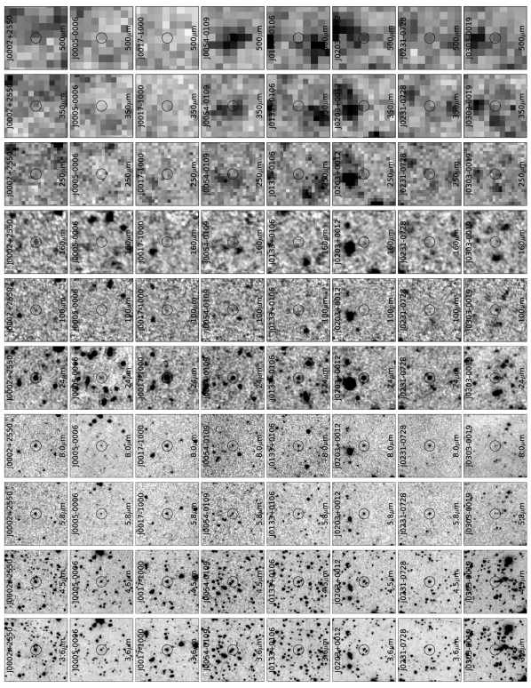
Figure A.1.— The Spitzer and Herschel images for all objects in this paper. Depicted are from left to right: 3.6 $\mu$m, 4.5 $\mu$m, 5.8 $\mu$m, 8 $\mu$m, 24 $\mu$m, 100 $\mu$m, 160 $\mu$m, 250 $\mu$m, 350 $\mu$m, and 500 $\mu$m. The individual panels show an area of 2′ $\times$ 2′ and the circle indicating the quasar position has a diameter of 20″. This excerpt is shown for guidance. See the online version of the journal for the remaining objects.

References

- Balog et al. (2013) Balog, Z., Müller, T., Nielbock, M., et al. 2013, Experimental Astronomy, 38
- Barvainis (1987) Barvainis, R. 1987, ApJ, 320, 537
- Beelen et al. (2006) Beelen, A., Cox, P., Benford, D. J., et al. 2006, ApJ, 642, 694
- Bendo et al. (2013) Bendo, G. J., Griffin, M. J., Bock, J. J., et al. 2013, MNRAS, 433, 3062
- Berta et al. (2011) Berta, S., Magnelli, B., Nordon, R., et al. 2011, A&A, 532, A49
- Bertoldi et al. (2003) Bertoldi, F., Carilli, C. L., Cox, P., et al. 2003, A&A, 406, L55
- Blain et al. (2013) Blain, A. W., Assef, R., Stern, D., et al. 2013, ApJ, 778, 113
- Carilli et al. (2001) Carilli, C. L., Bertoldi, F., Rupen, M. P., et al. 2001, ApJ, 555, 625
- Dai et al. (2012) Dai, Y. S., Bergeron, J., Elvis, M., et al. 2012, ApJ, 753, 33
- De Rosa et al. (2011) De Rosa, G., Decarli, R., Walter, F., et al. 2011, ApJ, 739, 56
- Diamond-Stanic et al. (2009) Diamond-Stanic, A. M., Fan, X., Brandt, W. N., et al. 2009, ApJ, 699, 782
- Elbaz et al. (2011) Elbaz, D., Dickinson, M., Hwang, H. S., et al. 2011, A&A, 533, A119
- Fan et al. (1999) Fan, X., Strauss, M. A., Schneider, D. P., et al. 1999, AJ, 118, 1
- Fan et al. (2000a) Fan, X., Strauss, M. A., Schneider, D. P., et al. 2000, AJ, 119, 1
- Fan et al. (2000b) Fan, X., White, R. L., Davis, M., et al. 2000, AJ, 120, 1167
- Fan et al. (2001) Fan, X., Narayanan, V. K., Lupton, R. H., et al. 2001, AJ, 122, 2833
- Fan et al. (2003) Fan, X., Strauss, M. A., Schneider, D. P., et al. 2003, AJ, 125, 1649
- Fan et al. (2004) Fan, X., Hennawi, J. F., Richards, G. T., et al. 2004, AJ, 128, 515
- Fan et al. (2006) Fan, X., Strauss, M. A., Richards, G. T., et al. 2006, AJ, 131, 1203
- Fazio et al. (2004) Fazio, G. G., Hora, J. L., Allen, L. E., et al. 2004, ApJS, 154, 10
- Freudling et al. (2003) Freudling, W., Corbin, M. R., & Korista, K. T. 2003, ApJ, 587, L67
- Fruchter & Hook (2002) Fruchter, A. S., & Hook, R. N. 2002, PASP, 114, 144
- Goto (2006) Goto, T. 2006, MNRAS, 371, 769
- Griffin et al. (2010) Griffin, M. J., Abergel, A., Abreu, A., et al. 2010, A&A, 518, L3
- Hao et al. (2011) Hao, H., Elvis, M., Civano, F., & Lawrence, A. 2011, ApJ, 733, 108
- Hasinger (2008) Hasinger, G. 2008, A&A, 490, 905
- Hewett et al. (2006) Hewett, P. C., Warren, S. J., Leggett, S. K., & Hodgkin, S. T. 2006, MNRAS, 367, 454
- Hines et al. (2006) Hines, D. C., Backman, D. E., Bouwman, J., et al. 2006, ApJ, 638, 1070
- Hönig & Kishimoto (2010) Hönig, S. F., & Kishimoto, M. 2010, A&A, 523, A27
- Houck et al. (2004) Houck, J. R., Roellig, T. L., van Cleve, J., Forrest, W. J., Herter, T., Lawrence, C. R., Matthews, K., et al. 2004, ApJS, 154, 18
- Isobe et al. (1986) Isobe, T., Feigelson, E. D., & Nelson, P. I. 1986, ApJ, 306, 490
- Iwamuro et al. (2004) Iwamuro, F., Kimura, M., Eto, S., et al. 2004, ApJ, 614, 69
- Jiang et al. (2006) Jiang, L., Fan, X., Hines, D. C., et al. 2006, AJ, 132, 2127
- Jiang et al. (2007) Jiang, L., Fan, X., Vestergaard, M., et al. 2007, AJ, 134, 1150
- Jiang et al. (2008) Jiang, L., Fan, X., Annis, J., et al. 2008, AJ, 135, 1057
- Jiang et al. (2010) Jiang, L., Fan, X., Brandt, W. N., et al. 2010, Nature, 464, 380
- Juarez et al. (2009) Juarez, Y., Maiolino, R., Mujica, R., et al. 2009, A&A, 494, L25
- Jun & Im (2013) Jun, H. D., & Im, M. 2013, arXiv:1310.3034
- Kaiser et al. (2010) Kaiser, N., Burgett, W., Chambers, K., et al. 2010, Proc. SPIE, 7733,
- Kennicutt (1998) Kennicutt, R. C., Jr. 1998, ARA&A, 36, 189
- Kurk et al. (2007) Kurk, J. D., Walter, F., Fan, X., et al. 2007, ApJ, 669, 32
- Kurk et al. (2009) Kurk, J. D., Walter, F., Fan, X., et al. 2009, ApJ, 702, 833
- Lawrence (1991) Lawrence, A. 1991, MNRAS, 252, 586
- Lawrence et al. (2007) Lawrence, A., Warren, S. J., Almaini, O., et al. 2007, MNRAS, 379, 1599
- Leipski et al. (2013) Leipski, C., Meisenheimer, K., Walter, F., et al. 2013, ApJ, 772, 103
- Lusso et al. (2013) Lusso, E., Hennawi, J. F., Comastri, A., et al. 2013, ApJ, 777, 86
- Lutz et al. (2008) Lutz, D., Sturm, E., Tacconi, L. J., et al. 2008, ApJ, 684, 853
- Lutz et al. (2011) Lutz, D., Poglitsch, A., Altieri, B., et al. 2011, A&A, 532, A90
- Mahabal et al. (2005) Mahabal, A., Stern, D., Bogosavljević, M., Djorgovski, S. G., & Thompson, D. 2005, ApJ, 634, L9
- Maiolino et al. (2003) Maiolino, R., Juarez, Y., Mujica, R., Nagar, N. M., & Oliva, E. 2003, ApJ, 596, L155
- Maiolino et al. (2007) Maiolino, R., Shemmer, O., Imanishi, M., et al. 2007, A&A, 468, 979
- McGreer et al. (2006) McGreer, I. D., Becker, R. H., Helfand, D. J., & White, R. L. 2006, ApJ, 652, 157
- McGreer et al. (2013) McGreer, I. D., Jiang, L., Fan, X., et al. 2013, ApJ, 768, 105
- Mor et al. (2009) Mor, R., Netzer, H., & Elitzur, M. 2009, ApJ, 705, 298
- Mor & Trakhtenbrot (2011) Mor, R., & Trakhtenbrot, B. 2011, ApJ, 737, L36
- Mor & Netzer (2012) Mor, R., & Netzer, H. 2012, MNRAS, 420, 526
- Nenkova et al. (2008) Nenkova, M., Sirocky, M. M., Nikutta, R., Ivezić, Ž., & Elitzur, M. 2008, ApJ, 685, 160
- Netzer et al. (2007) Netzer, H., Lutz, D., Schweitzer, M., et al. 2007, ApJ, 666, 806
- Netzer et al. (2013) Netzer, H., Mor, R., Trakhtenbrot, B., Shemmer, O., & Lira, P. 2013, arXiv:1308.0012
- Nguyen et al. (2010) Nguyen, H. T., Schulz, B., Levenson, L., et al. 2010, A&A, 518, L5
- Omont et al. (1996) Omont, A., McMahon, R. G., Cox, P., et al. 1996, A&A, 315, 1
- Ott (2010) Ott, S. 2010, Astronomical Data Analysis Software and Systems XIX, 434, 139
- Pascale et al. (2011) Pascale, E., Auld, R., Dariush, A., et al. 2011, MNRAS, 415, 911
- Petric et al. (2003) Petric, A. O., Carilli, C. L., Bertoldi, F., et al. 2003, AJ, 126, 15
- Pilbratt et al. (2010) Pilbratt, G. L., Riedinger, J. R., Passvogel, T., et al. 2010, A&A, 518, L1
- Priddey et al. (2003) Priddey, R. S., Isaak, K. G., McMahon, R. G., Robson, E. I., & Pearson, C. P. 2003, MNRAS, 344, L74
- Priddey et al. (2008) Priddey, R. S., Ivison, R. J., & Isaak, K. G. 2008, MNRAS, 383, 289
- Poglitsch et al. (2010) Poglitsch, A., Waelkens, C., Geis, N., et al. 2010, A&A, 518, L2
- Popesso et al. (2012) Popesso, P., Magnelli, B., Buttiglione, S., et al. 2012, arXiv:1211.4257
- Richards et al. (2006) Richards, G. T., Lacy, M., Storrie-Lombardi, L. J., et al. 2006, ApJS, 166, 470
- Rieke et al. (2004) Rieke, G. H., Young, E. T., Engelbracht, C. W., et al. 2004, ApJS, 154, 25
- Robson et al. (2004) Robson, I., Priddey, R. S., Isaak, K. G., & McMahon, R. G. 2004, MNRAS, 351, L29
- Romani et al. (2004) Romani, R. W., Sowards-Emmerd, D., Greenhill, L., & Michelson, P. 2004, ApJ, 610, L9
- Roseboom et al. (2010) Roseboom, I. G., Oliver, S. J., Kunz, M., et al. 2010, MNRAS, 409, 48
- Sanders et al. (1989) Sanders, D. B., Phinney, E. S., Neugebauer, G., Soifer, B. T., & Matthews, K. 1989, ApJ, 347, 29
- Savage & Oliver (2007) Savage, R. S., & Oliver, S. 2007, ApJ, 661, 1339
- Schartmann et al. (2008) Schartmann, M., Meisenheimer, K., Camenzind, M., et al. 2008, A&A, 482, 67
- Schlegel et al. (1998) Schlegel, D. J., Finkbeiner, D. P., & Davis, M. 1998, ApJ, 500, 525
- Sharp et al. (2001) Sharp, R. G., McMahon, R. G., Irwin, M. J., & Hodgkin, S. T. 2001, MNRAS, 326, L45
- Shen et al. (2011) Shen, Y., Richards, G. T., Strauss, M. A., et al. 2011, ApJS, 194, 45
- Stalevski et al. (2012) Stalevski, M., Fritz, J., Baes, M., Nakos, T., & Popović, L. Č. 2012, MNRAS, 420, 2756
- Treister & Urry (2006) Treister, E., & Urry, C. M. 2006, ApJ, 652, L79
- Treister et al. (2008) Treister, E., Krolik, J. H., & Dullemond, C. 2008, ApJ, 679, 140
- Ueda et al. (2003) Ueda, Y., Akiyama, M., Ohta, K., & Miyaji, T. 2003, ApJ, 598, 886
- Valiante et al. (2011) Valiante, R., Schneider, R., Salvadori, S., & Bianchi, S. 2011, MNRAS, 416, 1916
- Vanden Berk et al. (2001) Vanden Berk, D. E., Richards, G. T., Bauer, A., et al. 2001, AJ, 122, 549
- Venemans et al. (2012) Venemans, B. P., McMahon, R. G., Walter, F., et al. 2012, ApJ, 751, L25
- Walter et al. (2009) Walter, F., Riechers, D., Cox, P., et al. 2009, Nature, 457, 699
- Wang et al. (2007) Wang, R., Carilli, C. L., Beelen, A., et al. 2007, AJ, 134, 617
- Wang et al. (2008a) Wang, R., Wagg, J., Carilli, C. L., et al. 2008a, AJ, 135, 1201
- Wang et al. (2008b) Wang, R., Carilli, C. L., Wagg, J., et al. 2008b, ApJ, 687, 848
- Wang et al. (2010) Wang, R., Carilli, C. L., Neri, R., et al. 2010, ApJ, 714, 699
- Wang et al. (2011) Wang, R., Wagg, J., Carilli, C. L., et al. 2011, AJ, 142, 101
- Wang et al. (2013) Wang, R., Wagg, J., Carilli, C. L., et al. 2013, ApJ, 773, 44
- Werner et al. (2004) Werner, M. W., Roellig, T. L., Low, F. J., et al. 2004, ApJS, 154, 1
- Willott et al. (2003) Willott, C. J., McLure, R. J., & Jarvis, M. J. 2003, ApJ, 587, L15
- Willott et al. (2013) Willott, C. J., Omont, A., & Bergeron, J. 2013, ApJ, 770, 13
- Zheng et al. (2000) Zheng, W., Tsvetanov, Z. I., Schneider, D. P., et al. 2000, AJ, 120, 1607