Level density and $\gamma$-ray strength function in the odd-odd ²³⁸Np nucleus

Abstract

The level density and $\gamma$-ray strength function in the quasi-continuum of ²³⁸Np have been measured using the Oslo method. The level density function follows closely the constant-temperature level density formula and reaches 43 million levels per MeV at $S_{n}=5.488$ MeV of excitation energy. The $\gamma$-ray strength function displays a two-humped resonance at low-energy as also seen in previous investigations of Th, Pa and U isotopes. The structure is interpreted as the scissors resonance and has an average centroid of $\omega_{\rm SR}=2.26(5)$ MeV and a total strength of $B_{\rm SR}=10.8(12)\mu_{N}^{2}$, which is in excellent agreement with sum-rule estimates. The scissors resonance is shown to have an impact on the ²³⁷Np$(n,\gamma)^{238}$Np cross section.

I Introduction

Atomic nuclei in the actinide region are believed to be synthesized in explosive stellar environments purely by the rapid neutron-capture process. Therefore, to predict their abundances found on Earth ar07 ; kaeppler2011 , one has to know the various reaction rates for all isotopes including the ones with extreme neutron excess. Reaction rates are also vital for the modeling of future and existing nuclear reactors aliberti2006 ; chadwick2011 . It is particularly important to ensure a reliable extrapolation in cases where measured data are insufficient or lacking.

The ²³⁷Np isotope with a half-life of 2.14 million years is one of the main constituents in nuclear spent fuel. In the former US high-level waste repository in the Yucca Mountain, Nevada, about 40 tons of ²³⁷Np are stored esch2008 , and it is of great interest to find methods for transmuting this type of radioactive waste. In order to obtain high transmutation efficiency, the neutron fission-to-capture ratio should be determined for the particular isotope as function of neutron energy. Hence, accurate fission and capture cross sections are necessary to make reliable predictions aliberti2004 .

The nuclear level density and $\gamma$-ray strength function ($\gamma$SF) are important inputs in statistical Hauser-Feshbach reaction-rate calculations. These functions describe the average properties of excited nuclei in the quasi-continuum region, where the number of levels is too high to study individual states and their transitions. Here, the Oslo method Schiller00 ; Lars11 has been shown to be an excellent tool to determine simultaneously the level density and the $\gamma$-ray strength function ($\gamma$SF).

Recently, the Oslo method was applied to the ^231-233Th, ^232,233Pa and ^237-239U isotopes guttormsen2012 ; nld2013 ; gsf2014 . The level densities of all eight actinides follow closely the constant-temperature level density formula. Furthermore, a large scissors resonance (SR) was observed in the $\gamma$SF with a $\gamma$-energy centroid at $\omega_{\rm SR}\approx 2.4$ MeV. This extra $\gamma$ strength enhances the decay with $\gamma$ rays relative to other decay branches such as particle emission or fission.

One would expect that the SR is present throughout the region of well-deformed actinides. The n_TOF collaboration ntof2011 has recently reported on $(n,\gamma)$ experiments on the ²³⁴U, ²³⁷Np and ²⁴⁰Pu isotopes. They verify a low-energy structure in ²³⁵U and ²⁴¹Pu, but not in ²³⁸Np, a result which is rather surprising. The odd-odd ²³⁸Np nucleus has the same gross properties as other actinides, and the Oslo group has confirmed that the structure also appears in the odd-odd ²³²Pa nucleus gsf2014 . Thus, the n_TOF results on ²³⁸Np have triggered us to investigate this case further.

The main purpose of the present work is to search for the SR in ²³⁸Np and to determine the total level density and $\gamma$SF. Furthermore, we present for the first time $(n,\gamma$) cross-section from Hauser-Feshbach calculations using the measured level density and $\gamma$SF as inputs. The calculations are compared with known $(n,\gamma$) data from literature.

The manuscript is organized as follows. Section II describes briefly the experimental methods, and in Sect. III the extraction and normalization of the level density and $\gamma$SF are discussed. In Sect. IV the SR is presented, and extracted resonance parameters are compared to previous results and sum-rules estimates. In Sect. V the measured level density and $\gamma$SF are used as inputs to Hauser-Feshbach calculations in order to estimate $(n,\gamma)$ cross sections. Conclusions are drawn in Sect. VI.

II Experiment

The experiment was performed with the MC-35 Scanditronix cyclotron at the Oslo Cyclotron Laboratory (OCL). The ²³⁷Np target (thickness 0.200 mg/cm² and enrichment 99%), which had a carbon backing (thickness 0.020 mg/cm²), was bombarded with a 13.5 MeV deuteron beam. Particle-$\gamma$ coincidences were measured with the SiRi particle telescope and the CACTUS $\gamma$-detector system siri ; CACTUS .

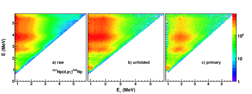
Figure 1: (Color online) Initial excitation energy $E$ versus $\gamma$-ray energy $E_{\gamma}$ from particle-$\gamma$ coincidences recorded with the ²³⁷Np$(d,p\gamma)^{238}$Np reaction. The raw $\gamma$-ray spectra (a) are first unfolded by the NaI response function (b) and finally the primary or first-generation $\gamma$-ray spectra (c) are extracted as function of excitation energy $E$. The excitation and $\gamma$ energy axis have dispersions of 14.0 keV/ch and 30.4 keV/ch, respectively.

The 64 SiRi telescopes were placed in backward direction covering eight angles from $\theta=126^{\circ}$ to $140^{\circ}$ relative to the beam axis. This configuration was chosen to reduce the intense elastically scattered deuterons and to obtain a broad and rather high spin distribution that matches better to the spin distribution of available states in the quasi-continuum. The front and back detectors have thicknesses of $130$ $\mu$m and $1550$ $\mu$m, respectively. The CACTUS array consists of 28 collimated $5^{\prime\prime}\times 5^{\prime\prime}$ NaI(Tl) detectors with a total efficiency of $15.2$% at $E_{\gamma}=1.33$ MeV.

The $E$ back detectors were used as master gates and the start for the time-to-digital-converter (TDC). One or more of the NaI detectors were used as individual TDC stops. In this way, prompt particle-$\gamma$ coincidences with background subtraction could be sorted event by event. The proton events were selected by setting proper 2-dimensional gates on the 64 $\Delta$E-E matrices. From the kinematics of the reaction, the proton energies deposited in the telescopes were translated into initial excitation energy $E$ in the residual ²³⁸Np nucleus.

Figure 1 shows the first main steps of the Oslo method. After sorting the data into a raw matrix of initial excitation energy versus the NaI energy signal (a), the matrix is unfolded Gutt96 using the NaI response function for each excitation bin (b). In panel (c) the first-generation (primary) $\gamma$-ray matrix $P(E,E_{\gamma})$ is shown. Here, an iterative subtraction technique was applied to separate out the distribution of the first-generation $\gamma$s from the total $\gamma$ cascade Gutt87 . The technique is based on the assumption that the $\gamma$ distribution is the same whether the levels were populated directly by the nuclear reaction or by $\gamma$ decay from higher-lying states. This assumption is necessarily fulfilled when states have the same relative probability to be populated by the two processes, since $\gamma$-branching ratios are properties of the levels themselves.

The first generation matrix $P$ is built from the total matrix $P_{{\rm gen}>0}$ of Fig. 1 (b), where all $\gamma$s of all cascade are included. The matrix with higher generations $P_{{\rm gen}>1}$ is obtained by weighting and summing the spectra at lower excitation energy. In principle, the first-generation matrix $P_{{\rm gen}=1}$ is identical to the proper weighting function and obtained by an iterative procedure described in detail in Ref. Gutt87 .

The number of counts in the second or higher-generation spectra $A_{{\rm gen}>1}$ has to relate to the counts of the total spectrum $A_{{\rm gen}>0}$. Since the $\gamma$ multiplicity of the first-generation spectra equals unity, we find

$$A_{{\rm gen}>1}=\frac{M_{\gamma}(E)-1}{M_{\gamma}(E)}A_{{\rm gen}>0}.$$ (1)

Provided, that we have a correct normalization of the counts in the $P_{{\rm gen}>1}$ matrix, the primary matrix is given by $P=P_{{\rm gen}>0}-P_{{\rm gen}>1}$. The average $\gamma$ multiplicity from initial excitation energy $E$ is given by

$$M_{\gamma}(E)=\frac{E}{\langle E_{\gamma}(E)\rangle},$$ (2)

where $\langle E_{\gamma}(E)\rangle$ is the centroid of the total $\gamma$ spectrum [Fig. 1 (b)] at $E$.

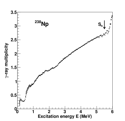
Figure 2: Gamma-ray multiplicity for $E_{\gamma}>0.45$ MeV as function of excitation energy $E$ in ²³⁸Np.

Figure 2 shows the $\gamma$ multiplicity for $E_{\gamma}>0.45$ MeV as function of initial excitation energy $E$. At the lower excitation energies, the multiplicity is seen to fluctuate since the decay routes become increasingly dependent on available levels of certain spin/parity and structure when approaching the ground state. Above $E=2-3$ MeV, the decay seems to reveal a statistical behavior. To proceed with the Oslo method, we use only the region $E=3.0-5.7$ MeV of the first generation matrix of Fig. 1 (c).

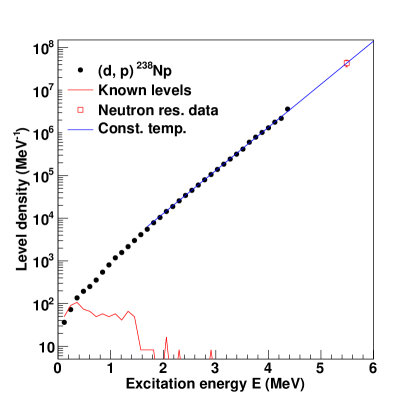
Figure 3: (Color online) Level density for ²³⁸Np. The experimental data are normalized to the level density of known discrete levels at low excitation energy $E$ (red solid line) and the level density extracted from known neutron resonance spacings $D_{0}$ at the neutron separation energy $S_{n}$. The connection between $\rho(S_{n})$ (the upper right data points) and our experimental data are made with a constant-temperature formula with $T_{\rm CT}=0.43$ MeV. The odd-odd ²³⁸Np nucleus has an extreme high level density of $\approx$ 43 million levels per MeV at the neutron separation energy of $S_{n}=5.488$ MeV.

According to the Brink hypothesis brink , the $\gamma$-ray transmission coefficient ${\cal{T}}$ is approximately independent of excitation energy. Thus, the first-generation matrix $P(E,E_{\gamma})$ may be factorized as follows:

$$P(E,E_{\gamma})\propto{\cal{T}}(E_{\gamma})\rho(E-E_{\gamma}),\$$ (3)

where $\rho(E-E_{\gamma})$ is the level density at the excitation energy after the first $\gamma$-ray has been emitted in the cascades. This factorization allows the disentanglement of the level density and $\gamma$-ray transmission coefficient. Note that no initial assumptions are made regarding to the functional form of ${\cal{T}}$ and $\rho$. However, the least-square fit of ${\cal{T}}\rho$ to the measured matrix $P$ [see Eq. (3)] determines only the functional form of ${\cal{T}}$ and $\rho$; if one solution of the functions ${\cal{T}}$ and $\rho$ is known, one may construct infinitely many identical fits to the $P(E,E_{\gamma})$ matrix by

$$\tilde{\rho}(E-E_{\gamma}) = A\exp[\alpha(E-E_{\gamma})]\,\rho(E-E_{\gamma}),$$ (4)

$$\tilde{{\mathcal{T}}}(E_{\gamma}) = B\exp(\alpha E_{\gamma}){\mathcal{T}}(E_{\gamma}).$$ (5)

The transformation parameters $A$, $\alpha$ and $B$ have then to be determined from other data, which is discussed in the next section.

Table 1: Parameters used to extract level density and $\gamma$SF (see text).

$S_{n}$	a	$E_{1}$	$\sigma(S_{n})$	$D_{0}$	$\rho(S_{n})$	$\rho(S_{n})_{\rm red}$	$\langle\Gamma_{\gamma}(S_{n})\rangle$
(MeV)	(MeV${}^{-1})$	(MeV)		(eV)	(106MeV-1)	(106MeV-1)	(meV)
5.488	25.96	-0.84	8.28	0.57(3)	43.0(78)	22	40.8(12)

III Normalization

We need to find the $A$ and $\alpha$ parameters of Eq. (4) in order to determine the level density. The two normalization points are determined at low excitation energy from the known level scheme ENSDF and at high energy from the density of neutron resonances following thermal ($n$, $\gamma$) capture at the neutron separation energy $S_{n}$. Here, the upper data point $\rho(S_{n})$ is estimated from $\ell=0$ neutron resonance spacings $D_{0}$ taken from RIPL-3 RIPL3 assuming a spin distribution GC

$$g(E=S_{n},I)\simeq\frac{2I+1}{2\sigma^{2}}\exp\left[-(I+1/2)^{2}/2\sigma^{2}\right].$$ (6)

The spin-cutoff parameter was determined from the global systematic study of level-density parameters by von Egidy and Bucurescu, who use a rigid-body moment of inertia approach egidy2 :

$$\sigma^{2}=0.0146A^{5/3}\frac{1+\sqrt{1+4aU}}{2a},$$ (7)

where $A$ is the mass number, $a$ is the level density parameter, $U=E-E_{1}$ is the intrinsic excitation energy, and $E_{1}$ is the back-shift parameter. Table 1 lists the $D_{0}$, $\sigma$ and $\rho$ values at $S_{n}$ used to determine the level density. The $a$ and $E_{1}$ parameters are taken from Ref. egidy2 . One should note that the spin distribution at such high excitation energies is not well known, and thus imposes a systematic uncertainty on our results.

Figure 3 demonstrates how the level density is normalized to the anchor points at low and high excitation energies. The level density follows closely the constant temperature formula with $\ln\rho\propto E/T_{\rm CT}$ as also measured for other Th, Pa and U isotopes nld2013 . It is interesting to see that only a small fraction of the levels, even at low excitation energies, have been observed in the odd-odd ²³⁸Np. The reason is of course the very high level density, e.g. at 1 MeV of excitation energy the average distance between levels is $\approx 1$ keV, only.

The level density is closely related to the entropy of the system, from which thermodynamic quantities such as temperature and heat capacity can be extracted. This will not be further elaborated here since the properties of the level density function observed for ²³⁸Np are very similar to those observed for ^237-239U  nld2013 .

The light-ion $(d,p)$ reaction used in this work may not populate the highest spins levels available in the nucleus, which in turn could influence the shape of the observed primary $\gamma$ spectra $P$. Since the transmission coefficient ${\cal{T}}$ is assumed to be independent of spin, the observed $P$ matrix should be fitted with the product ${\cal{T}}\rho_{\rm red}$, where the reduced level density is extracted by assuming a lower value of $\rho$ at $S_{n}$. Since there are uncertainties in the total $\rho(S_{n})$ through the estimate of $\sigma$ and also the actual spin distribution brought into the nuclear system by the specific reaction, the extracted slope of ${\cal{T}}$ becomes rather uncertain.

The parameter $B$ controls the scaling of the transmission coefficient ${\cal{T}}(E_{\gamma})$. Here we use the average, total radiative width $\langle\Gamma_{\gamma}\rangle$ at $S_{n}$ assuming that the $\gamma$-decay is dominated by dipole transitions. For initial spin $I$ and parity $\pi$, the width is given by ko90

$$\langle\Gamma_{\gamma}\rangle=\frac{1}{2\pi\rho(S_{n},I,\pi)}\sum_{I_{f}} \int_{0}^{S_{n}}{\mathrm{d}}E_{\gamma}B{\mathcal{T}}(E_{\gamma})$$ (8)

$$\times\rho(S_{n}-E_{\gamma},I_{f}),$$

where the summation and integration run over all final levels with spin $I_{f}$ that are accessible by $E1$ or $M1$ transitions with energy $E_{\gamma}$.

Since our spin distribution for the reaction is likely to be lower than the spin distribution of the available levels, the standard normalization procedure of the Oslo method Schiller00 ; voin1 to determine the $\alpha$ parameter for the transmission coefficient in Eq. (5) is not reliable. Instead we compare the $\gamma$SF with the extrapolation of known data from photo-nuclear reactions.

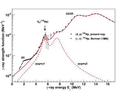
Figure 4: (Color online) Experimental $\gamma$SF from the present $(d,p)^{238}$Np experiment (black filled squares) compared with the estimated underlying $\gamma$SF (red curve), which represents the strength expected without the SR. The ($\gamma$, x) data (black filled triangles) are taken from Berman et al. berman1986 .

Table 2: Resonance parameters used for the $\gamma$SF extrapolation.

$\omega_{E1,1}$	$\sigma_{E1,1}$	$\Gamma_{E1,1}$	$\omega_{E1,2}$	$\sigma_{E1,2}$	$\Gamma_{E1,2}$	$T_{f}$	$\omega_{\rm pyg1}$	$\sigma_{\rm pyg1}$	$\Gamma_{\rm pyg1}$	$\omega_{\rm pyg2}$	$\sigma_{\rm pyg2}$	$\Gamma_{\rm pyg2}$
(MeV)	(mb)	(MeV)	(MeV)	(mb)	(MeV)	(MeV)	(MeV)	(mb)	(MeV)	(MeV)	(mb)	(MeV)
11.3	970	3.0	14.6	1520	4.4	0.2	5.5	50	0.7	7.5	60	1.4

The $\gamma$SF for dipole radiation can be calculated from the transmission coefficient ${\cal{T}}(E_{\gamma})$ by RIPL3

$$f(E_{\gamma})=\frac{1}{2\pi}\frac{{\mathcal{T}}(E_{\gamma})}{E_{\gamma}^{3}}.$$ (9)

These data are compared with the strength function derived from the cross section $\sigma$ of photo-nuclear reactions by RIPL3

$$f(E_{\gamma})=\frac{1}{3\pi^{2}\hbar^{2}c^{2}}\frac{\sigma(E_{\gamma})}{E_{\gamma}},$$ (10)

where the factor $1/3\pi^{2}\hbar^{2}c^{2}$ takes the value $8.6737\times 10^{-8}$ mb^-1MeV^-2. In Fig. 4 the $\gamma$SF derived from ²³⁷Np($\gamma$, x) cross section by Berman et al. berman1986 is shown (x means all possible ejectiles, as well as fission fragments). We assume that this strength do not vary much from ²³⁷Np to ²³⁸Np, as pointed out for the two ^236,238U isotopes gsf2014 .

Since our data cover $\gamma$ energies below $S_{n}$, we have to extrapolate the ($\gamma$, x) data to lower energies. For the double-humped giant electric dipole resonance (GEDR) we fit the data with two enhanced generalized Lorentzians (EGLO) as defined in RIPL RIPL3 , but with a constant temperature parameter of the final states $T_{f}$, in accordance with the Brink hypothesis. In addition the ($\gamma$, x) data berman1986 reveal a knee at around 7.5 MeV indicating a resonance-like structure (labeled pygmy2 in Fig. 4). We also note the steep flank of our $\gamma$SF data from 4 to 5 MeV of $\gamma$ energy. In order to match this increase in the $\gamma$SF another pygmy is postulated at around 5.5 MeV. The two pygmy resonances are described by simple Lorentzians:

$$f_{\rm pyg}=\frac{1}{3\pi^{2}\hbar^{2}c^{2}}\frac{\sigma_{\rm pyg}\Gamma_{\rm pyg}^{2}E_{\gamma}}{(E_{\gamma}^{2}-\omega_{\rm pyg}^{2})^{2}+\Gamma_{\rm pyg}^{2}E_{\gamma}^{2}}.$$ (11)

The sum of the two GEDR and the two pygmy $\gamma$SFs are shown as a solid red curve in Fig. 4. The four sets of resonance parameters are listed in Table 2.

We have also tested another approach of modeling the $\gamma$SF in the 4 - 8 MeV region. One broad Gaussian shape at 6.5 MeV gives approximatelly the same fit to the available data. However, we feel that there are no arguments to adopt a Gaussian shape for a resonance structure. Since the choice of one broad Lorentzian fails to reproduce the data, we keep to the assumption of two narrow pygmys as shown in Fig. 4.

Provided that the extrapolation in Fig. 4 (red solid curve) is reliable, we may assume that this $\gamma$SF represents the ”base line” with no additional strength from other resonances. Thus, we normalize the measured $\gamma$SF to this underlying background. Here, the $\alpha$ parameter is adjusted to obtain the right slope of the observed $\gamma$SF; the level density at $S_{n}$ had to be reduced from 43 to 22 million levels per MeV. The $B$ parameter was determined by use of Eq. (8) in order to reproduce the experimental $\gamma$ width $\langle\Gamma_{\gamma}\rangle$ listed in Table 1.

IV The scissors resonance

Figure 5 shows the $\gamma$SF where the assumed Lorentzian shape line of Fig. 4 has been subtracted. The observed structure, which is interpreted as the SR, is in accordance with previous observations in the ^231-233Th, ^232,233Pa and ^237-239U isotopes guttormsen2012 ; nld2013 ; gsf2014 . Thus, our findings is in strong disagreement with the $(n,\gamma)^{238}$Np results of the n_TOF group that found no evidence for the SR structure ntof2011 .

The SR is split into two components where the strengths of each component is given by a set of resonance parameters:

$$B=\frac{9\hbar c}{32\pi^{2}}\left(\frac{\sigma\Gamma}{\omega}\right).$$ (12)

The resonance parameters of the lower and upper component, as well as the total strength and average energy centroid are listed in Table 3.

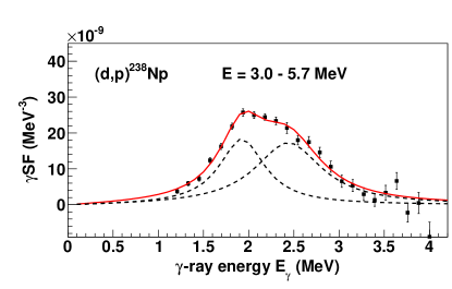
Figure 5: (Color online) The extracted $\gamma$SF for the scissors resonance in the quasi-continuum of ²³⁸Np.

We find that the separation in energy between the two components is much smaller than previously seen for Th, Pa and U gsf2014 ; $\Delta\omega_{\rm SR}=0.89(15)$ compared to $0.53(6)$ MeV for ²³⁸Np. In addition the higher lying component takes the main strength contrary to the other actinides where the low lying strength carried almost 2/3 of the strength. The total strength is the same as for the other actinides within the uncertainties.

Recent high quality measurements at the High-Intensity $\gamma$-ray Source (HI$\gamma$S) at the Triangle Universities Nuclear Laboratory (TUNL) has discovered more strength than for previous ($\gamma,\gamma^{\prime}$) measurements in this mass region heil1988 ; margraf1990 ; yevetska2010 . In ²³²Th a strength of $B_{\rm SR}=4.3(6)\mu_{N}^{2}$ at $\omega_{\rm SR}=2.5(4)$ MeV has been reported adekola2011 and for ²³⁸U there has been measured $B_{\rm SR}=8(1)\mu_{N}^{2}$ at $\omega_{\rm SR}=2.6(6)$ MeV hammond2012 .

Table 3: Scissors resonance parameters of ²³⁸Np and its sum-rule estimates [Eqs. (15) and (16), see text].

Deformation	Lower resonance				Upper resonance				Total		Sum rule
$\delta$	$\omega_{\rm SR,1}$	$\sigma_{\rm SR,1}$	$\Gamma_{\rm SR,1}$	$B_{\rm SR,1}$	$\omega_{\rm SR,2}$	$\sigma_{\rm SR,2}$	$\Gamma_{\rm SR,2}$	$B_{\rm SR,2}$	$\omega_{\rm SR}$	$B_{\rm SR}$	$\omega_{\rm SR}$	$B_{\rm SR}$
	(MeV)	(mb)	(MeV)	($\mu_{N}^{2}$)	(MeV)	(mb)	(MeV)	($\mu_{N}^{2}$)	(MeV)	($\mu_{N}^{2}$)	(MeV)	($\mu_{N}^{2}$)
0.25	1.95(4)	0.41(4)	0.61(5)	4.5(6)	2.48(6)	0.49(6)	0.90(10)	6.3(10)	2.26(5)	10.8(12)	2.2	9.9

During the last decades several SR models have been launched to explain the results of the ($\gamma$, ${\gamma}^{\prime}$) and ($e,e^{\prime}$) reactions heyde2011 . Very recent theoretical work on the scissors mode by Balbutsev, Molodtsova, and Schuck balbutsev2013 postulates a new additional mode, the isovector spin scissors mode, that may explain the appearent splitting of the scissors structure. However, the results of these calculations are rather qualitative at the present stage as pairing correlations are not taken into account. Furthermore, an important challenge is to explain why the splitting appears in the actinides and not in the rare-earth region.

In this work we have chosen the sum-rule approach lipparini1989 , which is a rather fundamental way to predict both $\omega_{\rm SR}$ and $B_{\rm SR}$ consistently. We follow the description of Enders et al. enders2005 with the exception that the ground-state moment of inertia will be replaced by the rigid-body moment of inertia. The outline for the quasi-continuum was recently presented gsf2014 , and we only give a summary of the formulas here.

The inversely and linearly energy-weighted sum rules are given by gsf2014

$$S_{+1} = \frac{3}{2\pi}\Theta_{\rm rigid}\delta^{2}\omega_{D}^{2}\left(\frac{Z}{A}\right)^{2}\xi~{}\left[\mu^{2}_{N}{\rm MeV}\right],$$ (13)

$$S_{-1} = \frac{3}{16\pi}\Theta_{\rm rigid}\left(\frac{2Z}{A}\right)^{2}~{}\left[\mu^{2}_{N}{\rm MeV}^{-1}\right].$$ (14)

The two sum rules can now be utilized to extract the SR centroid and strength:

$$\omega_{\rm SR} = \sqrt{S_{+1}/S_{-1}}$$ (15)

$$= |\delta|\omega_{D}\sqrt{2\xi},$$

$$B_{\rm SR} = \sqrt{S_{+1}S_{-1}}$$ (16)

$$= \frac{3}{4\pi}\left(\frac{Z}{A}\right)^{2}\Theta_{\rm rigid}|\delta|\omega_{D}\sqrt{2\xi}$$

$$= \frac{3}{4\pi}\left(\frac{Z}{A}\right)^{2}\Theta_{\rm rigid}\omega_{\rm SR}.$$

The rigid-body moment of inertia is taken as

$$\Theta_{\rm rigid}=\frac{2}{5}m_{N}r_{0}^{2}A^{5/3}(1+0.31\delta),$$ (17)

with $r_{0}=1.15$ fm and $\delta$ is the nuclear quadrupole deformation taken from goriely2009 . The reduction factor

$$\xi=\frac{\omega_{Q}^{2}}{\omega_{Q}^{2}+2\omega_{D}^{2}}$$ (18)

depends on the IVGDR and ISGQR frequencies of

$$\omega_{D} \approx (31.2A^{-1/3}+20.6A^{-1/6})(1-0.61\delta){\rm MeV},$$ (19)

$$\omega_{Q} \approx 64.7A^{-1/3}(1-0.3\delta){\rm MeV}.$$ (20)

The location of the IVGDR from systematics [Eq. (19)] gives $\omega_{D}=11.3$ MeV. However, the GEDR structures of Fig. 4 have clearly a higher average centroid. From the GEDR resonance parameters of Table 2 we find $\omega_{D}=13.4$ MeV, which we adopt for the sum-rule estimates.

The two last columns of Table 3 show the predicted $\omega_{\rm SR}$ and $B_{\rm SR}$ from the sum-rule estimates. Both values are in excellent agreement with our measurements.

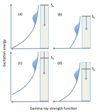
Figure 6: (Color online) Schematic view of how the SR (blue bump) influences the $\gamma$-decay rates. The scenarios are: (a) $E\approx S_{n}$ and high $S_{n}$, (b) $E\approx S_{n}$ and low $S_{n}$, (c) $E>S_{n}$ and high $S_{n}$, and (d) $E>S_{n}$ and low $S_{n}$. If the centroid of the $\gamma$ energies (arrow) overlaps with the centroid of the SR, the $\gamma$ branch may increase significantly (up to a factor of two). The ²³⁸Np nucleus with a relative high separation energy of $S_{n}=5.488$ MeV, corresponds to case (a). With neutron energies of several MeV, the influence of the SR will diminish.

V Calculations of the ($n,\gamma$) cross section

The $\gamma$SF in the quasi-continuum is the quantity that directly relates to the reaction rates in e.g. astrophysical environments. For example for the r-process, which involves nuclei with extreme $N/Z$ ratios, the decrease in neutron-separation energy with neutron number is expected to give an increasing impact from the SR on the reaction rates. The SR represents also an important ingredient for the simulations of fuel cycles for fast nuclear reactors.

In Fig. 6 the influence of the SR is schematically shown for four cases. It is obvious that if the initial state ”see” much of the high-energy tail of the $\gamma$SF, the low-lying SR strength will have less importance. This happens in panels (a) and (c). The higher overlap of the SR with the first-generations $\gamma$s appears in cases (b) and (d). In ²³⁸Np the binding energy is relatively high with $S_{n}=5.488$ MeV [case (a)], which means that only the high-energy part of the SR strength distribution comes into play.

In order to study the impact of the SR for ²³⁸Np, we have performed calculations of the $(n,\gamma)$ cross section with the TALYS code koning2008 . Experimental $(n,\gamma)$ cross sections are rather well known for ²³⁸Np, making this a good test ground for such calculations. In particular, a recent experiment at the DANCE facility esch2008 has provided data with small statistical errors for incoming neutron energies up to $\approx 300$ keV.

For the TALYS input we have used functions that decribe the observed level density and $\gamma$SF (data from Figs. 3 and 4, respectively). For the neutron optical-model potential, we have used the global parameterization of Koning and Delaroche koning2003 , but with adjusted values for the parameter $a_{V}$ using a scaling factor of $0.65$ to obtain agreement with the evaluated $s-$wave neutron strength function of $S_{0}=1.02(6)\times 10^{-4}$ mughabghab2006 .

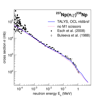
Figure 7: (Color online) Calculated ²³⁷Np$(n,\gamma)^{238}$Np cross section using level density and $\gamma$SF models in accordance with the data of this work. The predictions including the $M1$ scissors mode (blue curve) and without (dashed line) are compared with measured data from Esch et al. esch2008 (black squares) and Buleeva et al. buleeva1988 (open diamonds).

Figure 7 shows the results of the cross-section calculations. The TALYS output (blue curve) is in excellent agreement with the experimentally measured $(n,\gamma)$ cross sections from Refs. esch2008 ; buleeva1988 . The agreements for all neutron energies above the resonance region of $E_{n}\geq 300$ eV give confidence to the observed $\gamma$SF as well as the level density. The increase in cross section due to the SR reaches a maximum of $\approx 25$ % for 1-MeV incoming neutrons. The reason for the rather small influence of the $M1$ scissors resonance on the $(n,\gamma)$ cross section for this case is discussed in connection with Fig. 6; the inclusion of the SR has less impact because the high-energy part of the $\gamma$SF dominates the $\gamma$-decay probability. For the highest neutron energies in Fig. 7 ($E_{n}\geq 5$ MeV), the SR has no practical impact on the cross-section.

VI Conclusions

The level density and $\gamma$SF of ²³⁸Np have been determined using the Oslo method. The level density shows a constant-temperature behavior similar to other actinides as recently reported for ^231-233Th, ^232,233Pa and ^237-239U nld2013 ; gsf2014 .

We observe an excess in the $\gamma$SFs in the $E_{\gamma}=1-4$ MeV region, which is interpreted as the SR in the quasi-continuum. These findings are in contradiction with the n_TOF results from the $(n,\gamma)^{238}$Np reaction, but in agreement with expectations for the actinide region. The underlying strength of the SR has been subtracted by extrapolating the assumed strength from the tails of other resonances; the double humped GEDR and the two pygmy resonances. The SR shows a splitting into two components, however the two components are closer in energy than observed for the other actinides. The sum-rule applied to the quasi-continuum assuming a rigid-body moment of inertia, describes very well the centroid and strength of the SR.

The observed level density and $\gamma$SF have been used as inputs in Hauser-Feshbach calculations with the TALYS code. The agreement with previously measured $(n,\gamma)$ cross sections is very gratifying. The SR strength gives a maximum increase of 25 % on the calculated cross section for 1-MeV neutrons.

- (1) M. Arnould, S. Goriely, and K. Takahashi, Phys. Rep. 450, 97 (2007).
- (2) F. Käppeler et al., Rev. of Mod. Phys. 83, 157 (2011).
- (3) M.B. Chadwick et al., Nucl. Data Sheets 112, 2887 (2011).
- (4) G. Aliberti, G. Palmiotti, M. Salvatores, T.K. Kim, T.A. Taiwo, M. Anitescu, I. Kodeli, E. Sartori, J.C. Bosq, and J. Tommasi, Annals of Nuclear Energy 33, 700 (2006).
- (5) E-.I. Esch, R. Reifarth, E.M. Bond, T.A. Bredeweg, A. Couture, S.E. Glover, U. Greife, R.C. Haight, A.M. Hatarik, R. Hatarik, M. Jandel, T. Kawano, A. Mertz, J.M. O‘Donnell, R.S. Rundberg, J.M. Schwantes, J.L. Ullmann, D.J. Vieira, J.B. Wilhelmy, J.M. Wouters, and A.Alpizar-Vicente, Phys. Rev. C 77, 034309 (2008).
- (6) G. Aliberti, G. Palmiotti, M. Salvatores, and C.G. Stenberg, Nuclear Science and Engineering, 146, 13 (2004).
- (7) A. Schiller et al., Instrum. Methods Phys. Res. A 447, 498 (2000).
- (8) A.C. Larsen et al., Phys. Rev. C 83, 034315 (2011).
- (9) M. Guttormsen et al., Phys. Rev. Lett. 109, 162503 (2012).
- (10) M. Guttormsen et al., Phys. Rev. C 88, 024307 (2013).
- (11) M. Guttormsen et al., Phys. Rev. C 89, 014302 (2014).
- (12) C. Guerrero et al., Journal of the Korean Physical Society, 59, 1510 (2011).
- (13) M. Guttormsen, A. Bürger, T.E. Hansen, and N. Lietaer, Nucl. Instrum. Methods Phys. Res. A 648, 168 (2011).
- (14) M. Guttormsen et al., Phys. Scr. T 32, 54 (1990).
- (15) M. Guttormsen, T. S. Tveter, L. Bergholt, F. Ingebretsen, and J. Rekstad, Nucl. Instrum. Methods Phys. Res. A 374, 371 (1996).
- (16) M. Guttormsen, T. Ramsøy, and J. Rekstad, Nucl. Instrum. Methods Phys. Res. A 255, 518 (1987).
- (17) D.M. Brink, Ph.D. thesis, Oxford University, 1955.
- (18) Data extracted using the NNDC On-Line Data Service from the ENSDF database.
- (19) R. Capote et al., Reference Input Library, RIPL-2 and RIPL-3, available online at http://www-nds.iaea.org/RIPL-3/
- (20) A. Gilbert and A.G.W. Cameron, Can. J. Phys. 43, 1446 (1965).
- (21) T. von Egidy and D. Bucurescu, Phys. Rev. C 72, 044311 (2005); Phys. Rev. C 73, 049901(E) (2006).
- (22) J. Kopecky and M. Uhl, Phys. Rev. C 41 1941 (1990).
- (23) A. Voinov, M. Guttormsen, E. Melby, J. Rekstad, A. Schiller, and S. Siem, Phys. Rev. C 63, 044313 (2001).
- (24) B.L. Berman, J.T. Caldwell, E.J. Dowdy, S.S. Dietrich, P. Meyer, R.A. Alvarez, Phys. Rev. C 34, 2201 (1988); available at http://cdfe.sinp.msu.ru/services/unifsys/index.html.
- (25) R.D. Heil, H.H. Pitz, U.E.P. Berg, U. Kneissl, K.D. Hummel, G. Kilgus, D. Bohle, A. Richter, C. Wesselborg, P. von Brentano, Nucl. Phys. A 476, 39 (1988).
- (26) J. Margraf, A. Degener, H. Friedrichs, R.D. Heil, A. Jung, U. Kneissl, S. Lindenstruth, H.H. Pitz, H. Schacht, U. Seemann, R. Stock, C. Wesselborg, P. von Brentano, A. Zilges, Phys. Rev. C 42, 771 (1990).
- (27) O. Yevetska, J. Enders, M. Fritzsche, P. von Neumann-Cosel, S. Oberstedt, A. Richter, C. Romig, D. Savran, K. Sonnabend, Phys. Rev. C 81, 044309 (2010).
- (28) A.S. Adekola, C.T. Angell, S.L. Hammond, A. Hill, C.R. Howell, H.J. Karwowski, J.H. Kelley, and E. Kwan, Phys. Rev. C 83, 034615 (2011).
- (29) S.L. Hammond, A.S. Adekola, C.T. Angell, H.J. Karwowski E. Kwan, G. Rusev, A.P. Tonchev, W. Tornow, C.R. Howell, and J.H. Kelley, Phys. Rev. C 85, 044302 (2012).
- (30) K. Heyde, P. von Neumann-Cosel, A. Richter, Rev. Mod. Phys. 82, 2365 (2010), and references therein.
- (31) E.B. Balbutsev, I.V. Molodtsova, and P. Schuck, Phys. Rev. C 88, 014306 (2013).
- (32) E. Lipparini and S. Stringari, Phys. Rep. 175, 103 (1989).
- (33) J. Enders, P. von Neumann-Cosel, C. Rangacharyulu, and A. Richter, Phys. Rev. C 71, 014306 (2005).
- (34) S. Goriely, N. Chamel and J.M. Pearson, Phys. Rev. Lett. 102, 152503 (2009).
- (35) A.J. Koning, S. Hilaire, and M.C. Duijvestijn, TALYS-1.0, in Proceedings of the International Conference on Nuclear Data for Science and Technology, 22–27 April 2007, Nice, France, edited by O. Bersillon, F. Gunsing, E. Bauge, R. Jacqmin, and S. Leray (EDP Sciences, 2008), p. 211.
- (36) S. Goriely, S. Hilaire, and A.J. Koning, Astron. Astrophys. 487, 767 (2008).
- (37) A. J. Koning and J. P. Delaroche, Nucl. Phys. A713, 231 (2003).
- (38) S. F. Mughabghab, Atlas of Neutron Resonances, Fifth Edition, Elsevier Science (2006).
- (39) N.N. Buleeva, A.N. Davletshin, O.A. Tipunkov, S.V. Tikhonov, and V.A. Tolstikov, Atomnaya Energiya 65, 348 (1988).