Ground-based detection of the near-infrared emission from the dayside of WASP-5b ^,

Abstract

Context. Observations of secondary eclipses of hot Jupiters allow one to measure the dayside thermal emission from the planets’ atmospheres. The combination of ground-based near-infrared observations and space-based observations at longer wavelengths constrains the atmospheric temperature structure and chemical composition.

Aims. This work aims at detecting the thermal emission of WASP-5b, a highly irradiated dense hot Jupiter orbiting a G4V star every 1.6 days, in the $J$, $H$ and $K$ near-infrared photometric bands. The spectral energy distribution is used to constrain the temperature-pressure profile and to study the energy budget of WASP-5b.

Methods. We observed two secondary-eclipse events of WASP-5b in the $J$, $H$, $K$ bands simultaneously using the GROND instrument on the MPG/ESO 2.2 meter telescope. The telescope was in nodding mode for the first observation and in staring mode for the second observation. The occultation light curves were modeled to obtain the flux ratios in each band, which were then compared with atmospheric models.

Results. Thermal emission of WASP-5b is detected in the $J$ and $K$ bands in staring mode. The retrieved planet-to-star flux ratios are $0.168^{+0.050}_{-0.052}$% in the $J$ band and $0.269\pm 0.062$% in the $K$ band, corresponding to brightness temperatures of $2996^{+212}_{-261}$ K and $2890^{+246}_{-269}$ K, respectively. No thermal emission is detected in the $H$ band, with a 3-$\sigma$ upper limit of 0.166% on the planet-to-star flux ratio, corresponding to a maximum temperature of 2779 K. On the whole, our $J$, $H$, $K$ results can be explained by a roughly isothermal temperature profile of $\sim$2700 K in the deep layers of the planetary dayside atmosphere that are probed at these wavelengths. Together with Spitzer observations, which probe higher layers that are found to be at $\sim$1900 K, a temperature inversion is ruled out in the range of pressures probed by the combined data set. While an oxygen-rich model is unable to explain all the data, a carbon-rich model provides a reasonable fit but violates energy balance. The nodding-mode observation was not used for the analysis because of unremovable systematics. Our experience reconfirms that of previous authors: staring-mode observations are better suited for exoplanet observations than nodding-mode observations.

1 Introduction

Currently, the most fruitful results on the characterization of exoplanetary atmospheres come from transiting planets. Since the first transiting planet HD 209458b was discovered in 1999 (Charbonneau et al., 2000), more than 400 are confirmed. The orbital parameters of these planets are well constrained when transit observations were combined with radial velocity measurements. Precise planetary parameters such as mass and radius can be determined as well, which leads to a preliminary view of the internal structure of a planet, and thus to constrain the formation and evolutionary history of the planet (Guillot, 2005; Fortney et al., 2007). Furthermore, transiting planets provide unprecedented opportunities to probe their atmospheres, not only from wavelength-dependent effective radius variations determined from the transit (e.g.: Charbonneau et al., 2002), but also from differential planetary photon measurements from occultation (e.g.: Deming et al., 2005). In the latter case, the planet passes behind the star, which leaves us only stellar emission during a total eclipse.

As a subset of transiting planets that are exposed to high irradiation in close orbits around their host stars, hot Jupiters are the most favorable targets for thermal emission detection through secondary-eclipse observation. Their close orbits translate into a high occultation probability and frequency, while their high temperatures and large sizes make the planet-to-star flux ratio favorable. The first thermal emission detections of hot Jupiters have been achieved with the Spitzer Space Telescope (Deming et al., 2005; Charbonneau et al., 2005), which operates in the mid-infrared (MIR) wavelength range. Since then, a flood of such detections have been made with Spitzer observations, resulting in better knowledge of the chemical composition and thermal structure of the planetary atmosphere. Compared with the MIR, the near-infrared (NIR) wavelength range covers the peak of the spectral energy distribution (SED) of a planet and probes deeper into the atmosphere, therefore it can be used to constrain the atmosphere’s temperature structure and energy budget. While the Hubble Space Telescope has contributed much to the NIR observation on planetary secondary eclipses (e.g.: Swain et al., 2009a, b), now more observations with high precision are starting to come from ground-based mid-to-large aperture telescopes thanks to the atmospheric window in the NIR (e.g.: Croll et al., 2010a, b, 2011; Cáceres et al., 2011; Gillon et al., 2012). As shown for example by Madhusudhan (2012), these ground-based NIR measurements play a crucial role in determining the C/O ratio when combined with measurements from Spitzer observations.

WASP-5b was first detected by Anderson et al. (2008) as a hot Jupiter orbiting a 12.3 mag G4V type star every 1.628 days. Its mass and radius are derived to be 1.58 and 1.09 times of the Jovian values, respectively, which places it among the relatively dense hot Jupiters. Several follow-up transit observations have refined its density to be nearly the same as our Jupiter (Southworth et al., 2009; Fukui et al., 2011). Its host star has a slightly supersolar metallicity ([Fe/H]=+0.09$\pm$0.09), according to the high-resolution VLT/UVES spectroscopy of Gillon et al. (2009). The planetary orbit might have a marginally nonezero eccentricity based on the joint analysis of RV and photometric measurements (Gillon et al., 2009; Triaud et al., 2010; Husnoo et al., 2012). Triaud et al. (2010) studied the Rossiter-McLaughlin effect in the WASP-5 system and found a sky-projected spin-orbit angle compatible with zero ($\lambda$=12.1${}^{+10.0\circ}_{-8.0}$), indicating an orbit aligned with the stellar rotation axis. Furthermore, several studies focused on the potential transit-timing variations (TTVs) of this system. Gillon et al. (2009) first noticed that a linear fit cannot explain the transit ephemeris very well, which was later suspected to be caused by the poor quality of one timing (Southworth et al., 2009). Fukui et al. (2011) studied its TTVs in detail with an additional seven new transit observations and calculated a TTV rms of 68 s, only marginally larger than their mean timing uncertainty of 41 s. Hoyer et al. (2012) revisited this TTV signal by combining their nine new epochs and suggested that this TTV might be introduced by data uncertainties and systematics and not by gravitational perturbations.

From these intensive previous studies, WASP-5b has become an intriguing target for atmospheric characterization. It is not bloated, although it receives a relatively high irradiation of $\sim$2.1$\times$10⁹ erg s^-1 cm^-2 from its 5700 K (Gillon et al., 2009) host star (assuming a scaled major-axis $a/R_{*}$=5.37, Fukui et al., 2011), which would place it in the pM class in the scheme proposed by Fortney et al. (2008). Its proximity to the host star results in an equilibrium temperature of 1739 K assuming zero albedo and isotropic redistribution of heat across the whole planet, which could be as high as 2223 K in the extreme case of zero heat-redistribution. Its Ca II H and K line strength ($\log R^{\prime}_{\rm{HK}}$=$-$4.72$\pm$0.07, Triaud et al., 2010) suggests that the activity of the host star might prevent it from having an inverted atmosphere, given the correlation proposed by Knutson et al. (2010). Recently, Baskin et al. (2013) reported thermal detections from the Warm Spitzer mission, suggesting a weak thermal inversion or no inversion at all, with poor day-to-night energy redistribution.

In this paper, we present the first ground-based detections of thermal emission from the atmosphere of WASP-5b in the $J$ and $K$ bands through observations of secondary eclipse. Section 2 describes our observations of two secondary-eclipse events and the process of data reduction. Section 3 summarizes the approaches that we employed to remove the systematics and to optimally retrieve the flux ratios. In Sect. 4, we discuss remaining systematic uncertainties and orbital eccentricity, and we also offer explanations for the thermal emission of WASP-5b with planetary atmosphere models. Finally, we conclude in Sect. 5.

2 Observations and data reduction

We observed two secondary-eclipse events of WASP-5b with the GROND instrument mounted on the MPG/ESO 2.2 meter telescope at La Silla, Chile. This imaging instrument was designed primarily for the simultaneous observation of gamma-ray burst afterglows and other transients in seven filters: the Sloan $g^{\prime}$, $r^{\prime}$, $i^{\prime}$, $z^{\prime}$ and the NIR $J$, $H$, $K$ (Greiner et al., 2008). Dichroics are used to split the incident light into seven optical and NIR channels. Photons of the four optical channels are recorded by backside-illuminated $2048\times 2048$ E2V CCDs and stored in FITS files with four extensions. Photons of the three NIR channels are recorded by Rockwell HAWAII-1 arrays ($1024\times 1024$) and stored in a single FITS file with a size of $3072\times 1024$. The optical arm has a field of view (FOV) of $5.4\times 5.4$ arcmin² with a pixel scale of $0\aas@@fstack{\prime\prime}158$, while the NIR arm has an FOV of $10\times 10$ arcmin² with a pixel scale of $0\aas@@fstack{\prime\prime}60$. The guiding system employs a camera placed outside the main GROND vessel, $23^{\prime}$ south of the scientific FOV, which has a crucial impact on the choice of science pointing especially in the case of defocused observations. The capability of simultaneous optical-to-NIR multiband observation makes GROND a potentially good instrument for transit and occultation observations. For secondary-eclipse observations, the optical arm provides the opportunity to detect scattered light in favorable cases, while the NIR arm allows one to construct an SED for the thermal emission of a planetary atmosphere. In both of our observations, we only used the NIR arm (i.e. WASP-5 was not in the optical FOV) to include as many potential reference stars as possible in the NIR FOV.

The first secondary-eclipse event was observed continuously for four hours on UT July 26 2011, from 04:13 to 08:16. The observation was performed in an ABAB nodding pattern. Four exposures were taken on each nodding position during the first one third of the observing time, and 12 exposures each were taken in the remaining time. Each exposure was composed of two integrations of 3 seconds each (DIT=3 s), which were averaged together. However, the actual nodding pattern was far more complicated. The telescope operation GUI software crashed several times, and a new ABAB pattern was re-started on each crashed position. The resulting time series of each band was full of red noise, which is difficult to correct since systematic effects affect the recorded signals differently depending on location on the detector. Time series of each location did not cover the whole occultation duration, which makes the systematic correction problem even worse. Therefore we decided to discard this dataset in our further analysis. Only the result in the $K$ band is shown for comparison in Sect. 3 and Fig. 1.

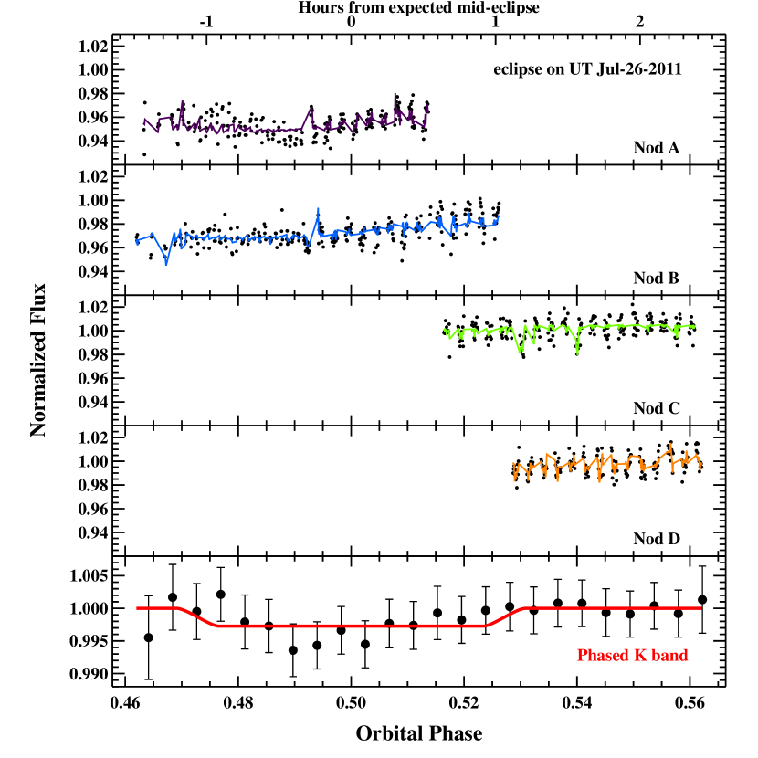
Figure 1: $K$-band occultation light-curve of WASP-5 observed on UT July 26 2011 (in nodding mode). As described in the text, instrumental crashes led to four groups of nods, none of which covered the whole eclipse. The top four panels show the raw light-curve for each nod, overplotted with the best-fit model. Bottom panel shows the phase-folded $K$-band light curve, which has been corrected for baseline trend and binned every 10 minutes for display purposes.

The second event of the secondary eclipse was observed continuously for 4.6 hours on UT September 8 2011, from 02:41 to 07:17 in staring mode. Before and after the science time series, the sky around the scientific FOV was measured using a 20-position dither pattern, which was used to construct the sky emission model in the subsequent reduction. During the science observation, four integrations of 3 seconds each were averaged into one exposure, resulting in 707 frames recorded and a duty cycle of $\sim$53%. The peak count level of the target star is well below the saturation level. The airmass started at 1.22, decreased to 1.02, and rose to 1.11 in the end; the seeing was unstable during the eclipse, ranging from $1^{\prime\prime}$ to $3^{\prime\prime}$ as measured from the point spread functions (PSFs) of the stars. The moon was illuminated around 82%, and had a minimum distance of 55^∘ to WASP-5 at the end of the observation. In the following text, we always refer to this second dataset unless specified otherwise.

We reduced the acquired data with our IDL pipeline in a standard way, which mainly makes use of NASA IDL Astronomy User’s Library. General image calibration steps include dark subtraction, read-out pattern removal, flat division, and sky subtraction. We made DARK master files by median-combining 20 individual dark-current measurements and subtracted them from all the raw images. To correct the electronic odd-even readout pattern along the X-axis, each dark-subtracted image was smoothed with a boxcar median filter and compared with the unsmoothed one. The amplitudes of readout patterns were obtained from the resulting difference image and were corrected in the unsmoothed dark-subtracted image. Finally, SKYFLAT master files were generated by median-combining 48 individual twilight sky flat measurements, which first had the star masked out and were then normalized and combined. The dark- and pattern-corrected images were divided by these SKYFLAT files for flat-field correction.

To eliminate the sky contribution in our staring-mode data, we constructed a sky emission model for each science image using the 20-position dithering sky measurements. These sky images were star-masked and normalized and then dark- and flat-calibrated in the same way as the science images. We median-combined on the sky stack images to generate basic sky emission models. The pre- and post-science sky models were scaled to the background level of each science image. A final sky model was created by combining the pre- and post-science sky models while taking the inverse square of the fitted $\chi^{2}$ as the weight. The final sky model was later subtracted from the corresponding science image. Due to the long time-scale of our observation, the sky is expected to be variable. Thus this sky correction is only a first-order correction. Nevertheless, it results in light curves of slightly better precision than the approach without sky subtraction, according to our experiment.

We performed aperture photometry on the calibrated images with the IDL DAOPHOT package. We first determined the locations of WASP-5 as well as several nearby comparison stars of similar brightness using IDL/FIND, which calculates the centroids by fitting Gaussians to the marginal $x$ and $y$ distributions. The FWHMs for each star, which were used to indicate the seeing during our observation, were calculated in a similar way. We carefully chose the best comparison-star ensemble to normalize the WASP-5 time series as follows: various combinations of comparison stars were tried. For each ensemble, time series of chosen comparison stars (as well as WASP-5) were individually normalized by the median of their out-of-eclipse flux levels, and then weighted-combined according to the inverse square of uncertainties. The ensemble that made the normalized WASP-5 light curve show the smallest scatter was considered as the optimal reference. We also experimented to find the best photometric results by placing 30 apertures on each star in a step of 0.5 pixel, each aperture again with 10 annuli of different sizes in a step of 1 pixel. The aperture and annulus that made reference-corrected WASP-5 light curve behave with the smallest scatter was chosen as the optimal aperture setting. As a result, we used six comparison stars for the $J$ band, three for the $H$ band, and four for the $K$ band. The aperture settings for the $J$, $H$, $K$ bands are (6.5, 13.5-22.0) pixels, (6.0, 6.0-19.0) pixels, (5.0, 7.0-19.0) pixels in the format of (aperture size, sky annulus inner/outer sizes), respectively.

Finally, we extracted the time stamp stored in the header of the FITS file. The default time stamp was the starting UTC time of each frame. We took into account the readout time and the arm-waiting time to make the final time stamp centered on the central point of each total integration. We converted this UTC time stamp into Barycentric Julian Date in the Barycentric Dynamical Time standard (BJD_TDB) using the IDL procedure written by Eastman et al. (2010).

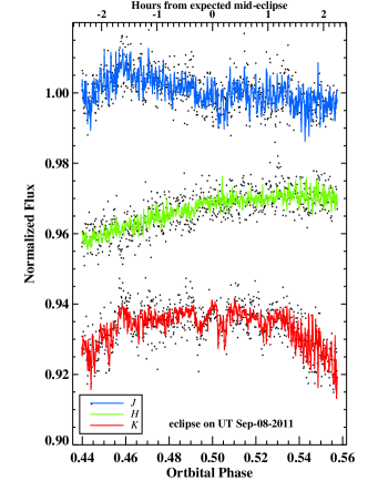
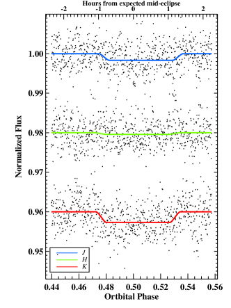
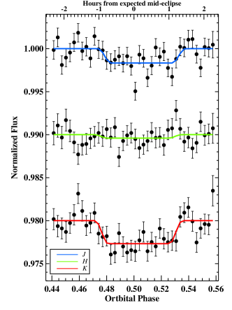
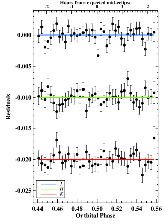
Figure 2: Near-infrared occultation light-curves of WASP-5 observed on UT Sep 08 2011 (in staring mode). Each panel from top to bottom shows for the $J$, $H$ and $K$ bands. Top left: raw light-curves overplotted with the best-fit models, which consist of a theoretical light-curve multiplied with a decorrelation function. Top right: light curves after baseline correction. Bottom left: light curves binned every seven minutes for display purposes. Bottom right: residuals of light-curve fitting.

Table 1: Results of the MCMC analysis on the secondary eclipse (Sep-08-2011) of WASP-5b

Parameter	Units	$J$ band	$H$ band	$K$ band
$T_{\rm{mid,occ}}$	BJD${}_{\rm{TDB}}-$2450000	5812.7249 ${}^{+0.0032}_{-0.0031}$	5812.7207 ${}^{+0.0031}_{-0.0031}$	5812.7215 ${}^{+0.0029}_{-0.0030}$
$\phi_{\rm{mid,occ}}$	…	0.5054 ${}^{+0.0020}_{-0.0019}$	0.5028 ${}^{+0.0019}_{-0.0019}$	0.5033 ${}^{+0.0018}_{-0.0018}$
$T_{\rm{offset}}$	minutes	12.6 ${}^{+4.7}_{-4.5}$	6.5 ${}^{+4.5}_{-4.5}$	7.7 ${}^{+4.2}_{-4.3}$
$F_{p}/F_{*}$	%	0.168 ${}^{+0.050}_{-0.052}$	0.041 ${}^{+0.039}_{-0.028}$, ¡0.166 (3$\sigma$)	0.269 ${}^{+0.062}_{-0.062}$
$T_{B}$	K	2996 ${}^{+212}_{-261}$	¡2779 (3$\sigma$)	2890 ${}^{+246}_{-269}$
$T_{58}$	days	0.1001 ${}^{+0.0063}_{-0.0070}$	…	0.1026 ${}^{+0.0054}_{-0.0058}$
$e\cos\omega$	…	0.0085 ${}^{+0.0030}_{-0.0029}$	…	0.0052 ${}^{+0.0028}_{-0.0029}$
$e\sin\omega$	…	-0.002 ${}^{+0.036}_{-0.044}$	…	0.013 ${}^{+0.030}_{-0.035}$
$e$	…	0.027 ${}^{+0.032}_{-0.015}$	…	0.025 ${}^{+0.024}_{-0.015}$
$|\omega|$	∘	72 ${}^{+11}_{-32}$	…	79 ${}^{+7}_{-24}$
Baseline	…	Equation (4)	Equation (5)	Equation (6)
$c_{0}$	…	1.00145 ${}^{+0.00031}_{-0.00033}$	1.00343 ${}^{+0.00022}_{-0.00015}$	1.00916 ${}^{+0.00052}_{-0.00053}$
$c_{1}$	…	0.01158 ${}^{+0.00012}_{-0.00012}$	0.004669 ${}^{+0.000053}_{-0.000077}$	-0.00173 ${}^{+0.00024}_{-0.00022}$
$c_{2}$	…	0.00808 ${}^{+0.00052}_{-0.00049}$	-0.009248 ${}^{+0.000027}_{-0.000048}$	-0.00450 ${}^{+0.00022}_{-0.00023}$
$c_{3}$	…	-0.00233 ${}^{+0.00027}_{-0.00028}$	0.00067 ${}^{+0.00015}_{-0.00010}$	-0.001958 ${}^{+0.00010}_{-0.00011}$
$c_{4}$	…	0.00715 ${}^{+0.00028}_{-0.00027}$	0.001877 ${}^{+0.000044}_{-0.000092}$	-0.00864 ${}^{+0.00012}_{-0.00011}$
$c_{5}$	…	-0.00760 ${}^{+0.00015}_{-0.00015}$	-0.000941 ${}^{+0.00010}_{-0.00014}$	0.0265 ${}^{+0.0046}_{-0.0043}$
$c_{6}$	…	-0.00209 ${}^{+0.00033}_{-0.00031}$	…	…
$c_{7}$	…	-0.00459 ${}^{+0.00014}_{-0.00014}$	…	…
$c_{8}$	…	-0.0246 ${}^{+0.0027}_{-0.0027}$	…	…

3 Light-curve analysis

As shown in the top left panel of Fig. 2, the WASP-5 light curves exhibited obvious red noise even after normalization by the composite reference light-curve as described above. Part of this red noise arises from instrumental systematics, such as different star locations on the detector, seeing variation (thus different number of pixels within the volume of the star’s FWHM), which can be inferred from the correlation between each parameter and the normalized flux (see Fig. 8–9 in the appendix). In the literature, some authors chose to construct a systematics model using out-of-eclipse data and applied these relationships to the whole light curve for correction (e.g. Croll et al., 2010a). This requires that the range of instrumental parameters during in-eclipse is repeatable in the out-of-eclipse data, otherwise it would lead to extrapolation. Since most of our instrumental parameters were not necessarily repeatable between in-eclipse and out-of-eclipse (e.g. slow drift of star location on the detector, variation of seeing), we decided to fit the whole light curve with an analytic occultation model multiplied by a baseline correction model.

We adopted the Mandel & Agol (2002) formulae without limb-darkening as our occultation model. System parameters such as period $P$, planet-to-star radius ratio $R_{p}/R_{*}$, inclination $i$, and scaled semi-major axis $a/R_{*}$ were obtained from Fukui et al. (2011) and were fixed in the formulae, while mid-occultation time $T_{\rm{mid}}$ and flux ratio $F_{p}/F_{*}$ were set as free parameters. The baseline detrending model was a sum of polynomials of star positions ($x$, $y$), seeings ($s$), airmass ($z$), and time ($t$). We varied the combination of these instrumental and atmospheric terms to generate different baseline models. We searched for the best-fit solutions by minimizing the chi-square:

$$\chi^{2}=\sum\limits_{i=1}^{N}\frac{[f_{i}(\mathrm{obs})-f_{i}(\mathrm{mod})]^{2}}{\sigma_{f,i}^{2}},$$ (1)

in which $f_{i}(\rm{obs})$ and $\sigma_{f,i}$ are the light-curve data and its uncertainty, while $f_{i}(\rm{mod})$ is the light-curve model, in the form of

$$f(\mathrm{mod})=E(T_{\mathrm{mid}},F_{p}/F_{*})B(x,y,s,z,t),$$ (2)

We experimented with a set of baseline models to find the model that can best remove the instrumental systematics. We calculated the Bayesian information criterion (BIC, Schwarz, 1978) for the results from different baseline models:

$$BIC=\chi^{2}+k\log(N),$$ (3)

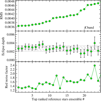
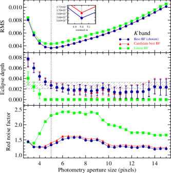
Figure 6: Dependence of $rms$, measured eclipse depth, and red noise factor on aperture size and reference ensemble for the $K$ band. The left panel shows the dependence on aperture size. The top subpanel displays the $rms$ of light-curve O–C residuals. The middle subpanel displays corresponding eclipse depths. The bottom subpanel displays the time-averaging red noise factor (i.e. $\beta_{2}$ as denoted in Sect. 3). The results derived from three cases of baseline functions (BF) are shown for comparison: the chosen best BF, a candidate BF that results in similar BIC to the best BF, and a linear BF that produces a poor fit. The vertical dotted line refers to the chosen aperture size, while the dash-shaded area refers to the 1-$\sigma$ confidence level of our reported result. The right panel shows the dependence of $rms$, measured eclipse depth, and red noise factor on different reference star ensembles. These ensembles have been sorted according to $rms$ for display purposes, with the best one being #1. The subpanels on the right are organized in the same manner as for the left.

where $k$ is the number of free parameters and $N$ is the number of data points. The baseline model that generated the smallest BIC value was considered as our final choice. With this approach, we used as few free parameters as possible to prevent overinterpreting the baseline function. In our experiments, linear baseline functions in most cases failed to fit the eclipse depth and produced very large BIC values. Among the baseline functions that have BICs similar to that of the chosen one, the measured eclipse depths agree well with each other (see e.g. Fig. 6 and 7). The final adopted baseline functions are

$$B_{J}=c_{0}+c_{1}x+c_{2}y+c_{3}xy+c_{4}x^{2}+c_{5}y^{2}+c_{6}s_{x}+c_{7}s_{y}+c_{8}t,$$ (4)

$$B_{H}=c_{0}+c_{1}x+c_{2}y+c_{3}xy+c_{4}y^{2}+c_{5}s_{x},$$ (5)

and

$$B_{K}=c_{0}+c_{1}xy+c_{2}x^{2}+c_{3}y^{2}+c_{4}s+c_{5}t,$$ (6)

where $s_{x}$ and $s_{y}$ refer to the FWHMs of marginal $x$ and $y$ distributions, respectively, while $s$ is their quadratic mean.

We employed the Markov chain Monte Carlo (MCMC) technique with the Metropolis-Hastings algorithm with Gibbs sampling to determine the posterior probability distribution function (PDF) for each parameter (see e.g. Ford, 2005, 2006). Following the approach of Gillon et al. (2010), only parameters in the analytic occultation model $E(T_{\rm{mid}},F_{p}/F_{*})$ are perturbed, while the coefficients of baseline function are solved using the singular value decomposition (SVD, Press et al., 1992) algorithm. At each MCMC step, a jump parameter was randomly selected, and the light curve was divided by the resulting analytic occultation model. The coefficients in the baseline function were then solved by linear least-squares minimization using the SVD. This jump was accepted if the resulting $\chi^{2}$ is lower than the previous $\chi^{2}$, or accepted according to the probability $\exp{(-\Delta\chi^{2}/2)}$ if the resulting $\chi^{2}$ is higher. We optimized the step scale so that the acceptance rate was $\sim$0.44 before a chain starts (Ford, 2006). After running a chain of MCMC, the first 10% links were discarded and the remaining were used to determine the best-fit values and uncertainties of jump parameters (as well as the baseline coefficients). Several chains were run to check that they were well mixed and converged using the Gelman & Rubin (1992) statistics. We adopted the median values of the marginalized distributions as the final parameter values and the 15.865%/84.135% values of the distributions as the 1-$\sigma$ lower/upper uncertainties, respectively.

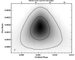
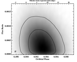
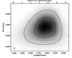
Figure 3: Joint probability distributions between mid-eclipse time and flux ratio from our MCMC analysis for the $J$ (left), $H$ (middle), and $K$ bands (right). The mid-eclipse time has been converted to phase in these plots. The contour lines mark the 68.3% ($1\sigma$) and 95.5% ($2\sigma$) confidence regions of the joint posterior distributions, respectively. The gray scale indicates the density of distributions.

We performed the MCMC-based light-curve modeling in three scenarios. In the first scenario, we tried to find the best-fit mid-occultation times and flux ratios. $T_{\rm{mid}}$ and $F_{p}/F_{*}$ were allowed to vary freely for the $J$ and $K$ bands. Since there was no detection in the $H$ band, we chose to adopt the PDF of $T_{\rm{mid}}$ coming from the $K$ band as a Gaussian prior. We first ran a chain of 1 000 000 links to find the scaling factors, since the photometric uncertainties might not represent the real uncertainties in the light curves well. We calculated the reduced chi-square ($\chi^{2}_{\nu}$) for the best-fit model and recorded the scaling factor $\beta_{1}$=$\sqrt{\chi^{2}_{v}}$. We then calculated the standard deviations for the best-fit residuals without binning, also for those with time bins ranging from 10 minutes to the ingress/egress duration of WASP-5b. The median value of the factor

$$\beta_{2}=\frac{\sigma_{N}}{\sigma_{1}}\sqrt{\frac{N(M-1)}{M}}$$ (7)

was recorded as the second scaling factor, where $N$ is the number of individual binned points, $M$ is the number of bins, $\sigma_{N}$ is the standard deviation of $N$-point binned residuals, and $\sigma_{1}$ is the un-binned version. These two scaling factors were multiplied with the original uncertainties to account for the under-/overestimated noise. Normally, the first scaling factor would make the fitting to have a reduced chi-square close to 1, while the second would take into account the time-correlated red noise. This approach has been widely applied in transit light-curve modeling (see e.g.: Pont et al., 2006; Winn et al., 2008). The derived ($\beta_{1}$, $\beta_{2}$) for the $J$, $H$, $K$ bands were (1.79, 1.28), (1.25, 1.46), (1.05,1.33), respectively. After rescaling the uncertainties, we ran another five chains of 1 000 000 links to finalize the modeling. The $J$-band flux ratio changed from 0.175$\pm$0.021% to 0.168${}^{+0.050}_{-0.052}$%, while the $K$-band flux ratio changed from 0.272$\pm$0.044% to 0.269$\pm$0.062%. The achieved light-curve quality for the $J$, $H$ and $K$ bands are 1847, 1813 and 1777 ppm per two-minute interval in terms of $rms$ of O–C (observed minus calculated) residuals. The estimated photon noise limits in the $J$, $H$, $K$ bands are 2.3$\times$10^-4, 2.4$\times$10^-4, and 3.7$\times$10^-4 per two-minute interval, respectively. This uncertainties rescaling has barely changed the best-fit values, but enlarged their uncertainties, thus decreased the detection significance. The derived jump parameters and coefficients for each band are listed in Table 1, while the posterior joint probability distributions between $T_{\rm{mid}}$ and $F_{p}/F_{*}$ are shown in Fig. 3.

In the second scenario, we changed the form of occultation model to $E(T_{58},T_{\rm{mid}},F_{p}/F_{*})$ so that we could fit the occultation duration $T_{58}$. Since our light curves are of poor quality, we decided to adopt the PDFs of $T_{\rm{mid}}$ and $F_{p}/F_{*}$ from the light-curve modeling in the first scenario as Gaussian priors input to the light-curve modeling in the second scenario. Another five chains of 1 000 000 links were run in search for the best-fit occultation duration of the $J$ and $K$ light curves. The $H$ band was not fitted because there was no detection. We obtained an occultation duration of $0.1001^{+0.0063}_{-0.0070}$ days for the $J$ band and $0.1026^{+0.0054}_{-0.0058}$ days for the $K$ band. They are both consistent with the primary transit duration $T_{14}$=0.1004 days (derived using parameters of Fukui et al., 2011) within their large uncertainties.

In the third scenario, we tried to model the light curves from the nodding observation (the Jul-26-2011 dataset) to directly compare the staring and nodding mode observations. The $J$ and $H$ bands in the nodding mode could fail to be fitted because of their extremely poor data quality. Thus we only modeled the $K$ band. The light curve was divided into four groups of nods according to their nodding positions. In the modeling, all four sub-light-curves share the same $F_{p}/F_{*}$ and have the mid-eclipse time fixed on the expected mid-point assuming zero eccentricity, while they are allowed to have different coefficients in the baseline from nod to nod. The adopted baseline function is

$$B_{K}=c_{0}+c_{1}x+c_{2}y+c_{3}xy+c_{4}x^{2}+c_{5}y^{2}.$$ (8)

We performed the MCMC-based modeling in the same manner as in the first scenario to find the scaling factors ($\beta_{1}$=1.47 and $\beta_{2}$=1.49) and to determine the flux ratio. This resulted in a flux ratio of 0.268$\pm$0.076% and $0.27^{+0.16}_{-0.15}$% for the unscaled and rescaled versions, respectively. The $rms$ of O–C residuals for this nodding light-curve is 4214 ppm per two-minute interval, twice as high as the staring mode. Considering that the nodding observations featured crashes, a better comparison would be using the un-crashed nodding pair. The $rms$ for the first 2-hour parts of nod A and B is 4738 ppm, while for the last 1-hour parts of nod C and D it is 2638 ppm. The main difference between these two un-crashed nodding pairs is their nodding pattern, that is, the locations of the same star on the detector are different, which results in instrumental systematics of very different levels. A location change also exists within one nodding pair. In contrast, the star’s location on the detector is relatively stable in the staring observation. Without the risk of introducing unexpected systematics from a different location, it is easier to model the light curve, which results in higher precision. This reconfirms that the staring mode is a better suited strategy than the nodding mode in exoplanet observations, which has been noted in several previous observations (e.g. for TrES-3b: de Mooij & Snellen, 2009; Croll et al., 2010b).

In addition to this analysis, we also examined our light curves to determine the correlations between measured eclipse depth and the choices of aperture size and reference ensemble (see Fig. 6 and 7 in the appendix). As the aperture radius increases, the $rms$ of light-curve O–C residuals first decreases to a minimum and then rises, which is expected because smaller apertures might lose partial stellar flux while larger apertures would include more sky noise. Correspondingly, the measured eclipse depth first changes greatly with the aperture size and then stabilizes when the aperture size approaches our chosen value. For aperture sizes that result in $rms$ similar to that of the chosen aperture, the measured eclipse depths agree well with our reported result within 1-$\sigma$ error bars. Furthermore, the measured eclipse depths derived from different combinations of reference stars are consistent with each other when they produce light curves with relatively low red noise. Therefore, we confirm that our choices of photometry and reference ensemble are ideal, in contrast, the measured eclipse depths are relatively insensitive to the choice of aperture size and reference ensemble.

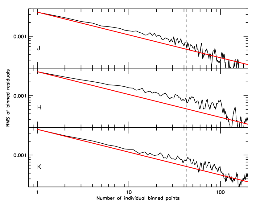
Figure 4: $RMS$ of the binned residuals v.s. bin size for the $J$, $H$ and $K$ occultation light-curves. The red lines shows the prediction for Gaussian white noise ($1/\sqrt{N}$). The vertical dashed line show the corresponding ingress/egress duration time. We can still see the strong effect of correlated noise in all three bands even after the baseline correction.

Table 2: Adopted parameters in the modeling process

Parameter	Units	Value	Ref.
Tmid,tran	BJDTDB	2454375.62510	a
Period	days	1.62843142	a
Inclination	degree	85.58	a
$a/R_{*}$	…	5.37	a
$R_{\rm{p}}/R_{*}$	…	0.1108	a
Eccentricity	…	0.	a
$\omega$	…	0.	a
$\log g_{*}$	cgs	4.395 ${}^{+0.043}_{-0.040}$	b
$T_{\rm{eff}}$	K	5700$\pm$100	b
$[$Fe/H$]$	dex	+0.09$\pm$0.09	b

4 Results and discussions

We list the derived jump parameters of our MCMC analysis in Table 1, along with the coefficients of the baseline functions from the modeling in the first scenario. Figure 1 shows the $K$-band light curve from the nodding observation (Jul-26-2011), while Fig. 2 shows all three light curves from the staring observation (Sep-08-2011). The adopted parameters that were used in our MCMC analysis are given in Table 2.

4.1 Correlated noise

In our MCMC analysis, we have propagated the uncertainties of the baseline detrending function into the PDFs of jump parameters by solving its coefficients at each MCMC step. We also tried to account for the red noise by rescaling the photometric uncertainties with the $\beta$ factors. The time averaging processes are shown in Fig.4. The $rms$ of the binned residuals clearly deviates from the predicted Gaussian white noise, as shown by the red lines, indicating the presence of correlated noise in our light curves. Here we employed another commonly used method (e.g.: Southworth, 2008), the ”prayer-bead” residual permutation method, which preserves the shape of time-correlated noise, to investigate whether there is still excess red noise that is not included in our MCMC analysis. Firstly, the best-fit model was removed from the light curve. The residuals were cyclically shifted from the $i$th to the $i$+1th positions (of the $N$ data points), while off-position data points in the end were wrapped at the beginning. Then the best-fit model was added back to the permuted residuals to form a new synthetic light curve. This synthetic light curve was then fitted in the same way as the real light curve, as described in Sect. 3. We inverted the light-curve sequence to perform another series of cycling, thus achieving 2$N$$-$1 synthetic light curves in total. We also calculated the median and 68.3% confidence level of the resulting distribution as the best-fit value and $1\sigma$ uncertainties.

This residual-permutation (RP)-based analysis leads to a flux ratio of $0.268^{+0.062}_{-0.054}$% for the $K$ band and $0.167^{+0.033}_{-0.038}$% for the $J$ band. The RP-based flux ratios have smaller uncertainties than those of the $\beta$-based MCMC analysis (0.269$\pm$0.062% and $0.168^{+0.050}_{-0.052}$%, correspondingly). The differences in best-fit values are very small. This indicates that our $\beta$-based MCMC analysis has included the potential impact from the time-correlated noise. We adopted the $\beta$-based MCMC results as our final results.

4.2 Orbital eccentricity

We obtain an average mid-occultation offset time of 10.5$\pm$3.1 minutes and an average occultation duration time of $0.1016^{+0.0041}_{-0.0045}$ days by combining values of the $J$ and $K$ bands with weights according to the inverse square of their uncertainties. The secondary eclipse of WASP-5b is expected to occur at phase $\phi$=0.5002 if it is in a circular orbit. This value has taken into account the delayed light travel time of $\sim$27 s (Loeb, 2005). However, our average mid-occultation time occurs at a delayed offset of 10.1$\pm$3.1 minutes to this expected phase, which might indicate a nonzero eccentricity. We used equations from Ragozzine & Wolf (2009) to derive the values of $e\cos\omega$ and $e\sin\omega$:

$$e\cos\omega\simeq\pi\Delta\phi/2$$ (9)

$$e\sin\omega=\frac{D_{\mathrm{II}}-D_{\mathrm{I}}}{D_{\mathrm{II}}+D_{\mathrm{I}}}\frac{\alpha^{2}-\cos^{2}i}{\alpha^{2}-2\cos^{2}i},$$ (10)

where $\alpha$=$(R_{*}/a+R_{\rm{p}}/a)/\sqrt{1-e^{2}}$, while $D_{\rm{II}}$ and $D_{\rm{I}}$ refer to the durations of secondary eclipse and primary transit. Thus $e\cos\omega$ and $e\sin\omega$ can be constrained if we can measure the mid-eclipse time and duration of a secondary eclipse with sufficient precision. We calculated an $e\cos\omega$=0.0067$\pm$0.0021 and an $e\sin\omega$=0.007$\pm$0.026. While the former parameter barely deviates from zero by $3\sigma$, the latter is consistent with zero within its large uncertainty. The 68.3% confidence level for eccentricity is $e$=0.020${}^{+0.019}_{-0.011}$, with corresponding argument of periastron $|\omega|$=71${}^{+11\circ}_{-31}$. Our derived eccentricity is only slightly larger than zero at a significance lower than $2\sigma$. From the previous radial velocity studies, Gillon et al. (2009) found a tentatively nonzero value of $e$=0.038${}^{+0.026}_{-0.018}$, while Husnoo et al. (2012) claimed that its eccentricity is compatible with zero ($e$=0.012$\pm$0.007) based on more RV measurements. Our result, derived from a different approach, lies between them and is consistent with both results within their errorbars. Recent Warm Spitzer measurements resulted in a mean value of $e\cos\omega$=0.0025$\pm$0.0012 (Baskin et al., 2013), which is 1.74$\sigma$ lower than our average value (c.f. 0.86$\sigma$ lower than our $K$-band result, see Table 1). However, we are cautious to draw any conclusion on nonzero eccentricity here. The shapes of our light curves are complicated due to the existence of instrumental and atmospheric systematics, as can be seen in Fig.2. It is very likely that these systematic effects bias the mid-eclipse time. Furthermore, the occultation duration is poorly constrained by our measurements.

4.3 Eclipse depths and brightness temperatures

To preliminarily probe the atmosphere, we first calculated the brightness temperatures corresponding to the measured flux ratios. We assumed blackbody emission for the planet and interpolated the stellar spectrum in the Kurucz stellar models (Kurucz, 1979) for the host star (using $T_{\rm{eff}}$=5700 K, $\log g$=4.395 and [Fe/H]=0.0). The blackbody spectrum and the stellar spectrum were both integrated over the bandpass of our three NIR bands individually. The blackbody temperature that yields the resulting flux ratio best-fit was adopted as the corresponding brightness temperature in each band. For the Sep-08-2011 secondary eclipse, the measured flux ratios are $0.168^{+0.050}_{-0.052}$% and 0.269$\pm$0.062% in the $J$ and $K$ band, and a $3\sigma$ upper limit of 0.166% in the $H$ band, which translates to brightness temperatures of $2996^{+212}_{-261}$ K, $2890^{+246}_{-269}$ K and $<2779$ K ($3\sigma$), respectively.

We used the same approach to calculate the brightness temperature of the Warm Spitzer data, where Baskin et al. (2013) reported 0.197$\pm$0.028% at 3.6 $\mu$m and 0.237$\pm$0.024% at 4.5 $\mu$m. In this way, the temperatures in the NIR and MIR were derived with the same stellar atmosphere models and parameters (c.f. Baskin et al., 2013). As a result, the Spitzer eclipse depths translate into brightness temperatures of 1982${}^{+117}_{-122}$ K and 1900${}^{+92}_{-94}$ K, respectively. The temperature derived from our NIR data ($\sim$2700 K) completely disagrees with that derived from the Warm Spitzer data ($\sim$1900 K).

4.4 Constraints on atmospheric properties

4.4.1 Atmospheric models

To investigate possible scenarios of the atmospheric properties, we modeled the emerging spectrum of the dayside atmosphere of WASP-5b using the exoplanetary atmospheric modeling and retrieval method of Madhusudhan & Seager (2009, 2010). Our model performs line-by-line radiative transfer in a plane-parallel atmosphere, with constraints on local thermodynamic equilibrium, hydrostatic equilibrium, and global energy balance. The pressure-temperature ($P$-$T$) profile and the molecular composition are free parameters of the model, allowing exploration of models with and without thermal inversions, and with oxygen-rich as well as carbon-rich compositions (Madhusudhan, 2012). The model includes all the primary sources of opacity expected in hydrogen-dominated atmospheres in the temperature regimes of hot Jupiters, such as molecular line absorption due to various molecules (H₂O, CO, CH₄, CO₂, HCN, C₂H₂, TiO, VO) and collision-induced absorption (CIA) due to H₂ (see Madhusudhan, 2012, for more details). The volume-mixing ratios of all the molecules are free parameters in the model. Given that the number of model parameters ($N$=10-14, depending on the C/O ratio) is much higher than the number of available data points, our goal is to nominally constrain the regions of model space favored by the data rather than determine a unique fit.

4.4.2 Constraints from our NIR data

Our observations place a stringent constraint on the temperature structure of the lower atmosphere of the planetary dayside. The $J$, $H$, and $K$ bands contain only weak molecular features due to spectroscopically dominant molecules in hot-Jupiter atmospheres. As such, photometric observations in these bands probe deep into the lower regions of the planetary atmosphere until the high pressures make the atmosphere optically thick (around $P\sim 0.1-1$ bar) due to H₂-H₂ CIA continuum absorption (Madhusudhan, 2012). Our observed brightness temperatures in the $J$, $H$, and $K$ bands can be explained by a roughly isothermal temperature profile of $\sim$2700 K in the lower atmosphere of WASP-5b, consistent with the fact that for highly irradiated hot Jupiters the dayside temperature structure at $\tau$$\sim$1 tends to be isothermal (Hansen, 2008; Madhusudhan & Seager, 2009; Guillot, 2010). In principle, our $J$ and $K$ band data allow for significantly higher temperatures, up to $\sim$3200 K, but our $H$-band observation rules out temperatures above $\sim$2700 K. As shown in Fig. 5, a blackbody spectrum of 2700 K representing the continuum blackbody of the lower atmosphere provides a reasonable fit to the $J$, $H$, $K$ data.

However, an isothermal temperature profile at $\sim$2700 K over the entire vertical extent of the atmosphere is unlikely. This would violate global energy balance since the planet would radiate substantially more energy than it receives. We assume that the internal source of energy is negligible compared to the incident irradiation (Burrows et al., 2008).

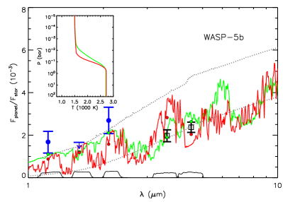
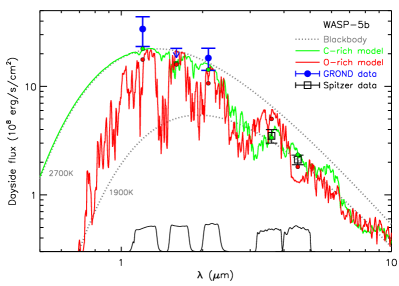
Figure 5: Dayside thermal emission spectrum from the hot Jupiter WASP-5b in terms of planet-to-star flux ratios (left) and planetary dayside flux (right). The blue circles with error bars at 1.26 $\mu$m and 2.15 $\mu$m and the upper-limit at 1.65 $\mu$m, show our measured planet-star flux ratios in the photometric $J$, $H$, and $K$ bands. The Spitzer photometric observations reported by Baskin et al. (2013) are shown at 3.6 $\mu$m and 4.5 $\mu$m (black squares). The dotted gray curves show two planetary blackbody spectra with temperatures of 1900 K and 2700 K. While our $J$, $H$, $K$ band data can be fit with a $\sim$2700 K blackbody spectrum, the Spitzer data is consistent with a $\sim$1900 K blackbody. The red and green curves show two model spectra of the dayside atmosphere of WASP-5b with oxygen-rich and carbon-rich compositions, respectively. The inset shows the corresponding pressure-temperature profiles without thermal inversions; a thermal inversion in the dayside atmosphere of WASP-5b is ruled out by the data. An oxygen-rich model is unable to explain all the data. On the other hand, while a carbon-rich model provides a good fit to the data, it radiates 70% more energy than the incident irradiation, which may be unphysical unless there are additional absorbing species in the atmosphere that are not accounted for in the current C-rich model. See Sect. 4.4 for discussion.

4.4.3 Constraints from NIR and Spitzer data

Additional constraints on the temperature profile and on the chemical composition of the dayside atmosphere of WASP-5b are obtained by combining our data with new photometric observations obtained with the Spitzer Space Telescope at 3.6 $\mu$m and 4.5 $\mu$m (Baskin et al., 2013).

Our data together with the Spitzer data rule out a thermal inversion in WASP-5b irrespective of its chemical composition, consistent with the finding of Baskin et al. (2013) based on the Spitzer data alone. The Spitzer data probe higher atmospheric layers than the ground-based data due to strong molecular absorption in the two Spitzer bands, and are consistent with brightness temperatures of $\sim$1900 K, which is much lower than the $\sim$2700 K temperatures in the ground-based channels. Consequently, the two data sets suggest temperatures decreasing outward in the atmosphere.

Previous work has shown that the Spitzer data also provide good diagnostics of the C/O ratio of the atmosphere as the bandpasses overlap with broad spectroscopic features of several dominant C- and O-bearing molecules (Madhusudhan, 2012). Chemical compositions of hot-Jupiter atmospheres can be extremely different depending on whether they are oxygen-rich (C/O $<$ 1) or carbon-rich (C/O$\geq$1). Whereas in O-rich atmospheres (e.g. of solar composition, with C/O = 0.5), H₂O and CO, and possibly TiO and VO, are the dominant sources of opacity, C-rich atmospheres are depleted in H₂O and abundant in CO, CH₄, HCN, and C₂H₂ (Madhusudhan et al., 2011b; Kopparapu et al., 2012; Madhusudhan, 2012; Moses et al., 2013).

We investigated both O-rich and C-rich scenarios in the present work and found that neither composition simultaneously provides a good fit to the data and satisfies energy balance, as shown in Fig. 5. However, the chemical composition is poorly constrained by the current data. First, we found that an O-rich solar composition atmosphere can neither fit all the data to within the 1-$\sigma$ errors nor satisfy energy balance; it radiates more energy than it receives. A composition with enhanced metallicity ($5\times$solar), but still O-rich, can satisfy energy balance, but still does not fit all the data, predicting the planet-star flux contrast at 3.6 $\mu$m to be $\gtrsim$3-$\sigma$ higher than the observed value, as shown in Fig. 5. On the other hand, a C-rich model can fit all the data reasonably well, but radiates 70% more energy than it receives from incident radiation, thereby violating global energy balance.

Both the O-rich and C-rich models were consistent with the lack of a thermal inversion in the planet. While the high chromospheric activity of the host star could destroy inversion-causing species in the atmosphere irrespective of its C/O ratio (Knutson et al., 2010; Baskin et al., 2013), a C-rich atmosphere would be naturally depleted in oxygen-rich inversion-causing compounds such as TiO and VO, which designates WASP-5b as a C2-class hot Jupiter in the classification of Madhusudhan (2012).

4.4.4 Possible scenarios and future prospects

Our data agree with two possible scenarios for WASP-5b: a carbon-rich and an oxygen-rich atmosphere. However, we caution that new observations are required to conclusively constrain its chemical composition.

The C-rich scenario, while providing a good fit to all available data, requires an explanation for the apparent energy excess in the emergent spectrum. This could be mitigated by an additional absorber in the atmosphere, which has high opacity blueward of the $J$ band ($\lesssim$1.1 $\mu$m) and/or a strong feature in the $H$ band ($\sim$1.5–1.8 $\mu$m). The presence of such a component is currently merely speculative, but could be seen or ruled out using follow-up spectroscopic observations, for instance with HST/WFC3. Such observations would additionally constrain the energy budget of the dayside atmosphere of WASP-5b.

The O-rich model satisfies global energy balance but does less well at simultaneously fitting the $J$, $H$, $K$ data and the Spitzer 3.6 $\mu$m point. One explanation is that the planet shows substantial temporal variability in its emerging spectrum, but the magnitude of the inferred variability seems implausibly high. Another possibility is that different systematic effects between the ground-based and Spitzer data bias the derived thermal emission measurements.

Spectroscopy with HST/WFC3 in the 1.1–1.7 $\mu$m bandpass would allow us to conclusively constrain the chemical composition of the atmosphere, since our two model spectra in Fig. 5 predict very different spectral shapes in that bandpass. In addition, observations of thermal phase curves with warm Spitzer (e.g. Knutson et al., 2009) will also allow us to place stringent constraints on the day-to-night energy redistribution, since all models fitting our current data predict extremely low redistributions implying strong day-to-night thermal contrasts.

5 Conclusions

We observed two secondary eclipses of WASP-5b simultaneously in the $J$, $H$ and $K$ bands with GROND on the MPG/ESO 2.2 meter telescope, one in nodding mode and the other in staring mode. Although we failed to extract useful results from the nodding-mode observation due to the associated complicated systematics, we did measure the occultation dips from the staring-mode observation with reasonable precision, reconfirming that the staring mode is more suited than the nodding mode for exoplanet observations.

We have successfully detected the thermal emission from the dayside of WASP-5b in the $J$ and $K$ bands, with flux ratios of $0.168^{+0.050}_{-0.052}$% and 0.269$\pm$0.062%, respectively. In the $H$ band we derived a 3-$\sigma$ upper limit of 0.166%. The brightness temperatures inferred from the $J$ and $K$ bands are consistent with each other ($2996^{+212}_{-261}$ K and $2890^{+246}_{-269}$ K, respectively), but the upper limit in the $H$ band rules out temperatures above 2779 K at $3\sigma$ level. While a slight difference might exist, together they indicate a roughly isothermal lower atmosphere of $\sim$2700 K. We modeled the GROND data together with the Warm Spitzer data using the spectral retrieval technique, ruling out a thermal inversion. We fit our data with two different models: an oxygen-rich atmosphere and a carbon-rich atmosphere. The O-rich model requires a very low day-to-night-side heat redistribution but satisfies energy balance. The C-rich model fits our data better, but violates energy balance in that it radiates 70% more energy than it receives. To constrain the chemical composition of WASP-5b and to distinguish atmospheric models, more observations in the NIR, in particular spectroscopy, are required.

Appendix A Additional figures

In this appendix, we present figures that show the dependence of measured eclipse depth on the choice of aperture radii and on the choice of different reference star combinations. We also display the correlations between raw light-curve flux and detrending parameters.

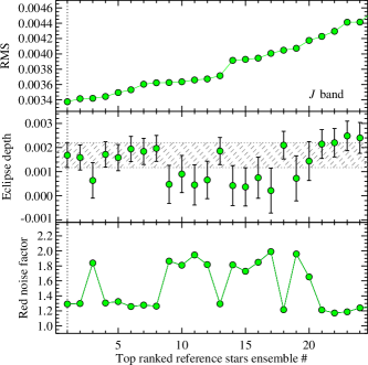
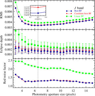
Figure 7: Dependence of $rms$, measured eclipse depth, and red noise factor on aperture size and reference ensemble for the $J$ band. The subpanels in this figure are organized in the same manner as Fig. 6.

Figure 8: Correlation between instrumental parameters (i.e. variables in the baseline function) and the normalized flux for the $K$ band. The first row shows the flux before baseline correction, while the second row shows the flux after baseline correction as a comparison. In these plots, $x$ and $y$ refer to the relative positions, and FWHM_x and FHWM_y refer to the full-width at half maximum of the marginalized PSF, both in pixels.

Figure 9: Correlation between instrumental parameters and the normalized flux for the $J$ band. The figure is displayed in the same manner as Fig. 8.