Radial and vertical flows induced by galactic spiral arms: likely contributors to our “wobbly Galaxy”

Abstract

In an equilibrium axisymmetric galactic disc, the mean galactocentric radial and vertical velocities are expected to be zero everywhere. In recent years, various large spectroscopic surveys have however shown that stars of the Milky Way disc exhibit non-zero mean velocities outside of the Galactic plane in both the Galactocentric radial and vertical velocity components. While radial velocity structures are commonly assumed to be associated with non-axisymmetric components of the potential such as spiral arms or bars, non-zero vertical velocity structures are usually attributed to excitations by external sources such as a passing satellite galaxy or a small dark matter substructure crossing the Galactic disc. Here, we use a three-dimensional test-particle simulation to show that the global stellar response to a spiral perturbation induces both a radial velocity flow and non-zero vertical motions. The resulting structure of the mean velocity field is qualitatively similar to what is observed across the Milky Way disc. We show that such a pattern also naturally emerges from an analytic toy model based on linearized Euler equations. We conclude that an external perturbation of the disc might not be a requirement to explain all of the observed structures in the vertical velocity of stars across the Galactic disc. Non-axisymmetric internal perturbations can also be the source of the observed mean velocity patterns.

1 Introduction

The Milky Way has long been known to possess spiral structure, but studying the nature and the dynamical effects of this structure has proven to be elusive for decades. Even though its fundamental nature is still under debate today, it has nevertheless started to be recently considered as a key player in galactic dynamics and evolution (e.g., Antoja et al. 2009; Quillen et al. 2011; Lépine et al. 2011; Minchev et al. 2012; Roskar et al. 2012 for recent works, or Sellwood 2013 for a review). However, zeroth order dynamical models of the Galaxy still mostly rely on the assumptions of a smooth time-independent and axisymmetric gravitational potential. For instance, recent determinations of the circular velocity at the Sun’s position and of the peculiar motion of the Sun itself all rely on the assumption of axisymmetry and on minimizing the non-axisymmetric residuals in the velocity field (Reid et al. 2009; McMillan & Binney 2010; Bovy et al. 2012; Schönrich 2012). Such zeroth order assumptions are handy since they allow us to develop dynamical models based on a phase-space distribution function depending only on three isolating integrals of motion, such as the action integrals (e.g., Binney 2013; Bovy & Rix 2013). Actually, an action-based approach does not necessarily have to rely on the axisymmetric assumption, as it is also possible to take into account the main non-axisymmetric component (e.g., the bar, see Kaasalainen & Binney 1994) by modelling the system in its rotating frame (e.g., Kaasalainen 1995). However the other non-axisymmetric components such as spiral arms rotating with a different pattern speed should then nevertheless be treated through perturbations (e.g., Kaasalainen 1994; McMillan 2013).

The main problem with such current determinations of Galactic parameters, through zeroth order axisymmetric models, is that it is not clear that assuming axisymmetry and dynamical equilibrium to fit a benchmark model does not bias the results, by e.g. forcing this benchmark model to fit non-axisymmetric features in the observations that are not present in the axisymmetric model itself. This means that the residuals from the fitted model are not necessarily representative of the true amplitude of non-axisymmetric motions. In this respect, it is thus extremely useful to explore the full range of possible effects of non-axisymmetric features such as spiral arms in both fully controlled test-particle simulations as well as self-consistent simulations, and to compare these with observations.

With the advent of spectroscopic and astrometric surveys, observational phase-space information for stars in an increasingly large volume around the Sun have allowed us to see more and more of these dynamical effect of non-axisymmetric components emerge in the data. Until recently, the most striking features were found in the solar neighbourhood in the form of moving groups, i.e. local velocity-space substructures shown to be made of stars of very different ages and chemical compositions (e.g., Chereul et al. 1998, 1999; Dehnen 1998; Famaey et al. 2005, 2007, 2008; Pompéia et al. 2011). Various non-axisymmetric models have been argued to be able to represent these velocity structures equally well, using transient (e.g., De Simone et al. 2004) or quasi-static spirals (e.g., Quillen & Minchev 2005; Antoja et al. 2011), with or without the help of the outer Lindblad resonance from the central bar (e.g., Dehnen 2000; Antoja et al. 2009; Minchev et al. 2010; McMillan 2013; Monari et al. 2013). The effects of non-axisymmetric components have also been analyzed a bit less locally by Taylor expanding to first order the planar velocity field in the cartesian frame of the Local Standard of Rest, i.e. measuring the Oort constants $A$, $B$, $C$ and $K$ (Kuijken & Tremaine 1994; Olling & Dehnen 2003), a procedure valid up to distances of less than 2 kpc. While old data were compatible with the axisymmetric values $C=K=0$ (Kuijken & Tremaine 1994), a more recent analysis of ACT/Tycho2 proper motions of red giants yielded $C=-10\,{\rm km}\,{\rm s}^{-1}\,{\rm kpc}^{-1}$ (Olling & Dehnen 2003). Using line-of-sight velocities of 213713 stars from the RAVE survey (Steinmetz et al. 2006; Zwitter et al. 2008; Siebert et al. 2011a; Kordopatis et al. 2013), with distances $d<2\,$kpc in the longitude interval $-140^{\circ}<l<10^{\circ}$, Siebert et al. (2011b) confirmed this value of $C$, and estimated a value of $K=+6\,{\rm km}\,{\rm s}^{-1}\,{\rm kpc}^{-1}$, implying a Galactocentric radial velocity gradient of $C+K=\partial V_{R}/\partial R\simeq-4\,{\rm km}\,{\rm s}^{-1}\,{\rm kpc}^{-1}$ in the solar suburb (extended solar neighbourhood, see also Williams et al. 2013). The projection onto the plane of the mean line-of-sight velocity as a function of distance towards the Galactic centre ($|l|<5^{\circ}$) was also examined by Siebert et al. (2011b) both for the full RAVE sample and for red clump candidates (with an independent method of distance estimation), and clearly confirmed that the RAVE data are not compatible with a purely axisymmetric rotating disc. This result is not owing to systematic distance errors as considered in Binney et al. (2013), because the geometry of the radial velocity flow cannot be reproduced by systematic distance errors alone (Siebert et al. 2011b; Binney et al. 2013). Assuming, to first order, that the observed radial velocity map in the solar suburb is representative of what would happen in a razor-thin disc, and that the spiral arms are long-lived, Siebert et al. (2012) applied the classical density wave description of spiral arms (Lin & Shu 1964; Binney & Tremaine 2008) to constrain their parameters in the Milky Way. They found that the best-fit was obtained for a two-armed perturbation with an amplitude corresponding to $\sim 15$% of the background density and a pattern speed $\Omega_{P}\simeq 19\,{\rm Gyr}^{-1}$, with the Sun close to the 4:1 inner ultra-harmonic resonance (IUHR). This result is in agreement with studies based on the location of moving groups in local velocity space (Quillen & Minchev 2005; Antoja et al. 2011; Pompéia et al. 2011). This study was advocated to be a useful first order benchmark model to then study the effect of spirals in three dimensions.

In three dimensions, observations of the solar suburb from recent spectroscopic surveys actually look even more complicated. Using the same red clump giants from RAVE, it was shown that the mean vertical velocity was also non-zero and showed clear structure suggestive of a wave-like behaviour (Williams et al. 2013). Measurements of line-of-sight velocities for 11000 stars with SEGUE also revealed that the mean vertical motion of stars reaches up to 10 km/s at heights of 1.5 kpc (Widrow et al. 2012), echoing previous similar results by Smith et al. (2012). This is accompanied by a significant wave-like North-South asymmetry in SDSS (Widrow et al. 2012; Yanny & Gardner 2013). Observations from LAMOST in the outer Galactic disc (within 2 kpc outside the Solar radius and 2 kpc above and below the Galactic plane) also recently revealed (Carlin et al. 2013) that stars above the plane exhibit a net outward motion with downward mean vertical velocities, whilst stars below the plane exhibit the opposite behaviour in terms of vertical velocities (moving upwards, i.e. towards the plane too), but not so much in terms of radial velocities, although slight differences are also noted. There is thus a growing body of evidence that Milky Way disc stars exhibit velocity structures across the Galactic plane in both the Galactocentric radial and vertical components. While a global radial velocity gradient such as that found in Siebert et al. (2011b) can naturally be explained with non-axisymmetric components of the potential such as spiral arms, such an explanation is a priori less self-evident for vertical velocity structures. For instance, it was recently shown that the central bar cannot produce such vertical features in the solar suburb (Monari et al. 2014). For this reason, such non-zero vertical motions are generally attributed to vertical excitations of the disc by external means such as a passing satellite galaxy (Widrow et al. 2012). The Sagittarius dwarf has been pinpointed as a likely culprit for creating these vertical density waves as it plunged through the Galactic disc (Gomez et al. 2013), while other authors have argued that these could be due to interaction of the disc with small starless dark matter subhalos (Feldmann & Spolyar 2013).

Here, we rather investigate whether such vertical velocity structures can be expected as the response to disc non-axisymmetries, especially spiral arms, in the absence of external perturbations. As a first step in this direction, we propose to qualitatively investigate the response of a typical old thin disc stellar population to a spiral perturbation in controlled test particle orbit integrations. Such test-particle simulations have revealed useful in 2D to understand the effects of non-axisymmetries and their resonances on the disc stellar velocity field, including moving groups (e.g., Antoja et al. 2009, 2011; Pompéia et al. 2011), Oort constants (e.g., Minchev et al. 2007), radial migrations (e.g., Minchev & Famaey 2010), or the dip of stellar density around corotation (e.g., Barros et al. 2013). Recent test-particle simulations in 3D have rather concentrated on the effects of the central bar (Monari et al. 2013, 2014), while we concentrate here on the effect of spiral arms, with special attention to mean vertical motions. In Sect. 2, we give details on the model potential, the initial conditions and the simulation technique, while results are presented in Sect. 3, and discussed in comparison with solutions of linearized Euler equations. Conclusions are drawn in Sect. 4.

2 Model

To pursue our goal, we use a standard test-particle method where orbits of massless particles are integrated in a time-varying potential. We start with an axisymmetric background potential representative of the Milky Way (Sect. 2.1), and we adiabatically grow a spiral perturbation on it within $\sim 3.5$ Gyr. Once settled, the spiral perturbation is kept at its full amplitude. This is not supposed to be representative of the actual complexity of spiral structure in real galaxies, where self-consistent simulations indicate that it is often coupled to a central bar and/or a transient nature with a lifetime of the order of only a few rotations. Nevertheless, it allows us to investigate the stable response to an old enough spiral perturbation ($\sim 600\,$Myr to $1\,$Gyr in the self-consistent simulations of Minchev et al. 2012). The adiabatic growth of this spiral structure is not meant to be realistic, as we are only interested in the orbital structure of the old thin disk test population once the perturbation is stable.

We generate initial conditions for our test stellar population from a discrete realization of a realistic phase-space distribution function for the thin disc defined in integral-space (Sect 2.2), and integrate these initial conditions forward in time within a given time-evolving background+spiral potential (Sect. 2.3). We then analyze the mean velocity patterns seen in configuration space, both radially and vertically, and check whether such patterns are stable within the rotating frame of the spiral.

2.1 Axisymmetric background potential

The axisymmetric part of the Galactic potential is taken to be Model I of Binney & Tremaine (2008). Its main parameters are summarized in Table 1 for convenience. The central bulge has a truncated power-law density of the form

$$\rho_{b}(R,z)=\rho_{b0}\times\left(\frac{\sqrt{R^{2}+(z/q_{b})^{2}}}{a_{b}}\right)^{-\alpha_{b}}{\rm exp}\left(-\frac{R^{2}+(z/q_{b})^{2}}{r_{b}^{2}}\right)$$ (1)

where $R$ is the Galactocentric radius within the midplane, $z$ the height above the plane, $\rho_{b0}$ the central density, $r_{b}$ the truncation radius, and $q_{b}$ the flattening. The total mass of the bulge is $M_{b}=5.18\times 10^{9}{\rm M}_{\odot}$.

The stellar disc is a sum of two exponential profiles (for the thin and thick discs):

$$\rho_{d}(R,z)=\Sigma_{d0}\times\left(\sum_{i=1}^{i=2}\frac{\alpha_{d,i}}{2z_{d,i}}{\rm exp}\left(-\frac{|z|}{z_{d,i}}\right)\right){\rm exp}\left(-\frac{R}{R_{d}}\right)$$ (2)

where $\Sigma_{d0}$ is the central surface density, $\alpha_{d,1}$ and $\alpha_{d,2}$ the relative contributions of the thin and thick discs, $z_{d,1}$ and $z_{d,2}$ their respective scale-heights, and $R_{d}$ the scale-length. The total mass of the disc is $M_{d}=5.13\times 10^{10}{\rm M}_{\odot}$.The disc potential also includes a contribution from the interstellar medium of the form

$$\rho_{g}(R,z)=\frac{\Sigma_{g}}{2z_{g}}\times{\rm exp}\left(-\frac{R}{R_{g}}-\frac{R_{m}}{R}-\frac{|z|}{z_{g}}\right)$$ (3)

where $R_{m}$ is the radius within which there is a hole close to the bulge region, $R_{g}$ is the scale-length, $z_{g}$ the scale-height, and $\Sigma_{g}$ is such that it contributes to 25% of the disc surface density at the galactocentric radius of the Sun.

Finally, the dark halo is represented by an oblate two-power-law model with flattening $q_{h}$, of the form

$$\rho_{h}(R,z) = \rho_{h0}\times\left(\frac{\sqrt{R^{2}+(z/q_{h})^{2}}}{a_{h}}\right)^{-\alpha_{h}}\times$$ (4)

$$\left(1+\frac{\sqrt{R^{2}+(z/q_{h})^{2}}}{a_{h}}\right)^{\alpha_{h}-\beta_{h}}.$$

Table 1: Parameters of the axisymmetric background model potential (Binney & Tremaine 2008)

Parameter	Axisymmetric potential
$M_{b}({\rm M}_{\odot})$	$5.18\times 10^{9}$
$M_{d}({\rm M}_{\odot})$	$5.13\times 10^{10}$
$M_{h,<100\ \mathrm{kpc}}({\rm M}_{\odot})$	$6.\times 10^{11}$
$\rho_{b0}({\rm M}_{\odot}\,{\rm pc}^{-3})$	$0.427$
$a_{\mathrm{b}}(\ \mathrm{kpc})$	$1.$
$r_{b}(\ \mathrm{kpc})$	$1.9$
$\alpha_{b}$	$1.8$
$q_{b}$	$0.6$
$\Sigma_{d0}+\Sigma_{g}({\rm M}_{\odot}\,{\rm pc}^{-2})$	1905.
$R_{d}(\ \mathrm{kpc})$	2.
$R_{g}(\ \mathrm{kpc})$	4.
$R_{m}(\ \mathrm{kpc})$	4.
$\alpha_{d,1}$	$14/15$
$\alpha_{d,2}$	$1/15$
$z_{d,1}(\ \mathrm{kpc})$	0.3
$z_{d,2}(\ \mathrm{kpc})$	1.
$z_{g}(\ \mathrm{kpc})$	0.08
$\rho_{h0}({\rm M}_{\odot}\,{\rm pc}^{-3})$	0.711
$a_{h}(\ \mathrm{kpc})$	$3.83$
$\alpha_{h}$	$-2.$
$\beta_{h}$	$2.96$
$q_{h}$	$0.8$

The potential is calculcated using the GalPot routine (Dehnen & Binney 1998). The rotation curve corresponding to this background axisymmetric potential is displayed in Fig. 1. For radii smaller than $11$ kpc, the total rotation curve (black line) is mostely infuenced by the disc (blue dashed line) and above by the halo (red dotted line).

Figure 1: Rotation curve corresponding to the background axisymmetric potential

2.2 Initial conditions

The initial conditions for the test stellar population are set from a discrete realization of a phase-space distribution function (Shu 1969, Bienaymé & Séchaud 1997) which can be written in integral space as:

$$f(E_{R},L_{z},E_{z})=\frac{\Omega\,\rho_{d}}{\sqrt{2}\kappa\pi^{\frac{3}{2}}\sigma^{2}_{R}\sigma_{z}}\exp\left(\frac{-(E_{R}-E_{c})}{\sigma^{2}_{R}}-\frac{E_{z}}{\sigma^{2}_{z}}\right)$$ (5)

in which the angular velocity $\Omega$, the radial epicyclic frequency $\kappa$ and the disc density in the plane $\rho_{d}$ are all functions of $L_{z}$, being taken at the radius $R_{c}(L_{z})$ of a circular orbit of angular momentum $L_{z}$. The scale-length of the disc is taken to be 2 kpc as for the background potential. The energy $E_{c}(L_{z})$ is the energy of the circular orbit of angular momentum $L_{z}$ at the radius $R_{c}$. Finally, the radial and vertical dispersions $\sigma^{2}_{R}$ and $\sigma^{2}_{z}$ are also function of $L_{z}$ and are expressed as:

$$\sigma^{2}_{R}=\sigma^{2}_{R_{\odot}}\exp\left(\frac{2R_{\odot}-2R_{c}}{R_{\sigma_{R}}}\right),$$ (6)

$$\sigma^{2}_{z}=\sigma^{2}_{z_{\odot}}\exp\left(\frac{2R_{\odot}-2R_{c}}{R_{\sigma_{z}}}\right)$$ (7)

where $R_{\sigma_{R}}/R_{d}=R_{\sigma_{z}}/R_{d}=5$. The initial velocity dispersions thus decline exponentially with radius but at each radius, it is isothermal as a function of height. These initial values are set in such a way as to be representative of the old thin disc of the Milky Way after the response to the spiral perturbation. Indeed, the old thin disc is the test population we want to investigate the response of.

From this distribution function, $4\times 10^{7}$ test particle initial conditions are generated in a 3D polar grid between $R=4$ kpc and $R=15$ kpc (see Fig. 2). This allows a good resolution in the solar suburb. Before adding the spiral perturbation, the simulation is run in the axisymmetric potential for two rotations ($\sim 500$ Myr), and is indeed stable.

Figure 2: Initial conditions. Left panel: Number of stars per ${\rm kpc}^{2}$ (surface density) within the Galactic plane as a function of $R$. Right panel: Stellar density as a function of $z$ at $R=8$ kpc.

Figure 3: Positions of the main radial resonances of the spiral potential. $\Omega(R)=v_{c}(R)/r$ is the local circular frequency, and $v_{c}(R)$ is the circular velocity. The $2:1$ ILR occurs along the curve $\Omega(R)-\kappa/2$, where $\kappa$ is the local radial epicyclic frequency. The inner $4:1$ IUHR occurs along the curve $\Omega(R)-\kappa/4$.

Figure 4: Positions of the 4:1, 6:1 and 8:1 vertical resonances. When $\Omega-\Omega_{P}=\nu/n$, where $\nu$ is the vertical epicyclic frequency, the star makes precisely $n$ vertical oscillations along one rotation within the rotating frame of the spiral.

2.3 Spiral perturbation and orbit integration

In 3D, we consider a spiral arm perturbation of the Lin-Shu type (Lin & Shu 1964; see also Siebert et al. 2012) with a sech² vertical profile (a pattern that can be supported by three-dimensional periodic orbits, see e.g. Patsis & Grosbøl 1996) and a small ($\sim 100$ pc) scale-height:

$$\Phi_{s}(R,\theta,z)=-A\cos\left[m\left(\Omega_{P}t-\theta+\frac{\ln(R)}{\tan p}\right)\right]{\rm sech}^{2}\left(\frac{z}{z_{0}}\right)$$ (8)

in which $A$ is the amplitude of the perturbation, $m$ is the spiral pattern mode ($m=2$ for a 2-armed spiral), $\Omega_{P}$ is the pattern speed, $p$ the pitch angle, and $z_{0}$ is the spiral scale-height. The edge-on shapes of orbits of these thick spirals are determined by the vertical resonances existing in the potential.

The parameters of the spiral potential used in our simulation are inspired by the analytic solution found in Siebert et al. (2012) using the classical 2D Lin-Shu formalism to fit the radial velocity gradient observed with RAVE (Siebert et al. 2011b). The parameters used here are summarized in Table 2. The amplitude $A$ which we use corresponds to 1% of the background axisymmetric potential at the Solar radius (3% of the disc potential). The positions of the main radial resonances, i.e. the 2:1 inner Lindblad resonance (ILR) and 4:1 IUHR, are illustrated in Fig. 3. The presence of the 4:1 IUHR close to the Sun is responsible for the presence of the Hyades and Sirius moving groups in the local velocity space at the Solar radius (see Pompéia et al. 2011), associated to square-shaped resonant orbital families in the rotating spiral frame. Vertical resonances are also displayed in Fig. 4.

Such a spiral perturbation can grow naturally in self-consistent simulations of isolated discs without the help of any external perturber (e.g. Minchev et al. 2012). As we are interested hereafter in the global response of the thin disc stellar population to a quasi-static spiral perturbation, we make sure to grow the perturbation adiabatically by multiplying the above potential perturbation by a growth factor starting at $t\approx 0.5$ Gyr and finishing at $t\approx 3.5$ Gyr: $\epsilon(t)=\frac{1}{2}(\tanh(1.7\times t-3.4)+1)$. The integration of orbits is performed using a fourth order Runge-Kutta algorithm run on Graphics Processing Units (GPUs). The growth of this spiral is not meant to be realistic, as we are only interested in the orbital structure of the old thin disk once the perturbation is stable.

Table 2: Parameters of the spiral potential and location of the main resonances

Parameter	Spiral potential
$m$	2
$A$ (km2 s-2)	1000
$p$ (deg)	-9.9
$z_{0}(\ \mathrm{kpc})$	0.1
$\Omega_{P}(\,{\rm km}{\rm s}^{-1}\ \mathrm{kpc}^{-1})$	18.6
$R_{\rm ILR}(\ \mathrm{kpc})$	1.94
$R_{\rm IUHR}(\ \mathrm{kpc})$	7.92
$R_{\mathrm{CR}}(\ \mathrm{kpc})$	11.97

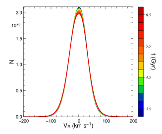
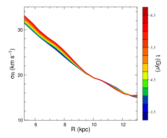
Figure 5: Left panel: Histogram of galactocentric radial velocities as a function of time. Right panel: time evolution of the $\sigma_{R}(R)$ profile averaged over all azimuths. The colour-scale indicates the time-steps in Gyr.

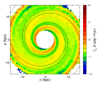
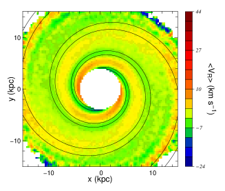
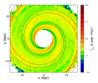
Figure 6: Top-left panel: Mean galactocentric radial velocity $\langle v_{R}\rangle$ as a function of position in the Galactic plane soon after the adiabatic growth of the spiral ($t=4\,$Gyr). Isocontours of the spiral potential are overplotted, corresponding to 80% of the minimum of the perturber potential, and thus delimiting the region where the spiral potential is between 80% and 100% of its minimum (or maximum in absolute value). Top right: Same at $t=5\,$Gyr. Everything is plotted here within the rotating frame of the spiral, so that the spiral does not move from one snapshot to the other. Bottom left: Same at $t=6\,$Gyr. Bottom right: Same at the final time-step $t=6.5\,$Gyr.

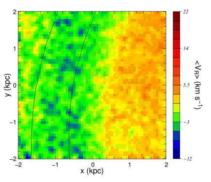
Figure 7: Galactocentric radial velocities in the solar suburb, centered at $(R,\theta)=(8\,{\rm kpc},26^{\circ})$ at $t=4\,$Gyr. On this plot, the Sun is centered on $(x,y)=(0,0)$, positive $x$ indicates the direction of the Galactic centre, and positive $y$ the direction of galactic rotation (as well as the sense of rotation of the spiral pattern). The spiral potential contours overplotted (same as on Fig. 6, delimiting the region where the spiral potential is between 80% and 100% of its absolute maximum) would correspond to the location of the Perseus spiral arm in the outer Galaxy. This Figure can be qualitatively compared to Fig. 4 of Siebert et al. (2011b) and Fig. 3 of Siebert et al. (2012).

3 Results

3.1 Radial velocity flow

The histogram of individual galactocentric radial velocities, $v_{R}$, as well as the time-evolution of the radial velocity dispersion profile starting from $t=3.5\,$Gyr (once the steady spiral pattern is settled) are plotted on Fig. 5. It can be seen that these are reasonably stable, and that the mean radial motion of stars is very close to zero (albeit slightly positive). Our test population is thus almost in perfect equilibrium.

However, due to the presence of spiral arms, the mean galactocentric radial velocity $\langle v_{R}\rangle$ of our test population is non-zero at given positions within the frame of the spiral arms. The map of $\langle v_{R}\rangle$ as a function of position in the plane is plotted on Fig. 6, for different time-steps (4 Gyr, 5 Gyr, 6 Gyr and 6.5 Gyr). Within the rotating frame of the spiral pattern, the locations of these non-zero mean radial velocities are stable over time: this means that the response to the spiral perturbation is stable, even though the amplitude of the non-zero velocities might slightly decrease with time. Within corotation, the mean $\langle v_{R}\rangle$ is negative within the arms (mean radial motion towards the Galactic centre) and positive (radial motion towards the anticentre) between the arms. Outside corotation, the pattern is reversed. This is exactly what is expected from the Lin-Shu density wave theory (see, e.g., Eq. 3 in Siebert et al. 2012).

If we place the Sun at $(R,\theta)=(8\,{\rm kpc},26^{\circ})$ in the frame of the spiral, we can plot the expected radial velocity field in the Solar suburb (Fig. 7). We see that the galactocentric radial velocity is positive in the inner Galaxy, as observed by Siebert et al. (2011b), because the inner Galaxy in the local suburb corresponds to an inter-arm region located within the corotation of the spiral. Observations towards the outer arm (which should correspond to the Perseus arm in the Milky Way) should reveal negative galactocentric radial velocities.

An important aspect of the present study is the behaviour of the response to a spiral perturbation away from the Galactic plane. The spiral perturbation of the potential is very thin in our model ($z_{0}=100\,$pc) but as we can see on Figs. 8 and 9, the radial velocity flow is not varying much as a function of $z$ up to five times the scale-height of the spiral perturber. This justifies the assumption made in Siebert et al. (2012) that the flow observed at $\sim 500\,$pc above the plane was representative of what was happening in the plane. Nevertheless, above these heights, the trend seems to be reversed, probably due to the higher eccentrities of stars, corresponding to different guiding radii. This could potentially provide a useful observational constraint on the scale height of the spiral potential, a test that could be conducted with the forthcoming surveys.

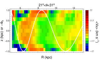
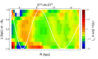
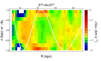
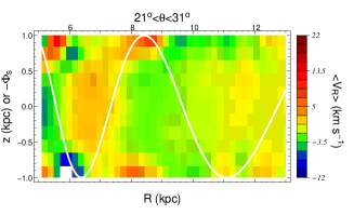
Figure 8: Top left panel: Mean galactocentric radial velocity at $t=4\,$Gyr in the meridional $(R,z)$-plane for $21^{\circ}<\theta<31^{\circ}$ (within the frame of the spiral). The white line indicates the location of spiral arms, in terms of overdensities and underdensities generating the spiral potential (normalized $-\Phi_{s}$, i.e. spiral arms are located at the peaks). Top right: Same at $t=5\,$Gyr. Bottom left: Same at $t=6\,$Gyr. Bottom right: Same at the final time-step $t=6.5\,$Gyr.

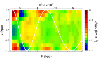
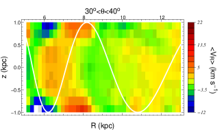
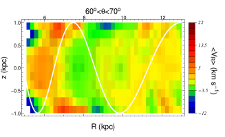
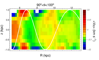
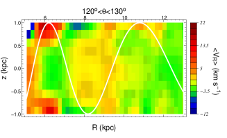
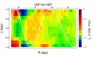
Figure 9: Same as Fig. 8, but for six different azimuths at a fixed time ($t=6\,$Gyr).

3.2 Non-zero mean vertical motions

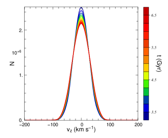
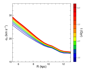
Figure 10: Left panel: Histogram of vertical velocities as a function of time . Right panel: time evolution of the $\sigma_{z}(R)$ profile averaged over all azimuths.

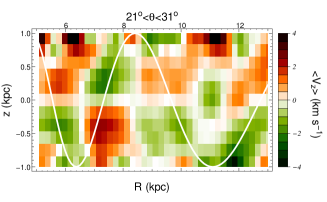
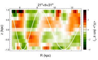
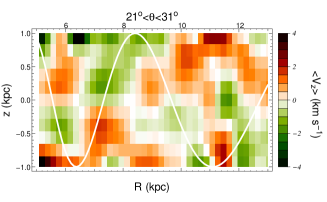
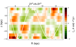
Figure 11: Top-left panel: Mean vertical velocity $\langle v_{z}\rangle$ at $t=4\,$Gyr in the meridional $(R,z)$-plane for $21^{\circ}<\theta<31^{\circ}$ (within the frame of the spiral). Top right: Same at $t=5\,$Gyr. Bottom left: Same at $t=6\,$Gyr. Bottom right: Same at the final time-step $t=6.5\,$Gyr. This figure can be compared at the qualitative level to Fig. 13 of Williams et al. (2013).

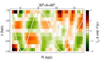
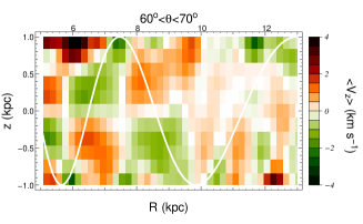
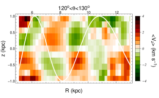
Figure 12: Same as Fig. 11, but for six different azimuths at a fixed time ($t=6\,$Gyr).

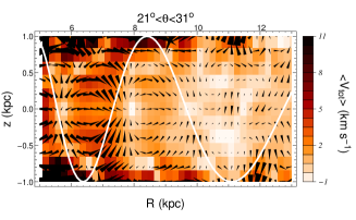
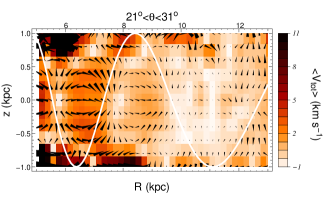
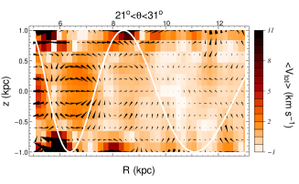
Figure 13: Top-left panel: “Total” velocity flow in the meridional $(R,z)$-plane $\sqrt{\langle v_{R}\rangle^{2}+\langle v_{z}\rangle^{2}}$ at $t=4\,$Gyr for $21^{\circ}<\theta<31^{\circ}$. Arrows indicate the direction of the velocity flow $\vec{\langle v\rangle}=\langle v_{R}\rangle\vec{1}_{R}+\langle v_{z}\rangle\vec{1}_{z}$. Top right: Same at $t=5\,$Gyr. Bottom left: Same at $t=6\,$Gyr. Bottom right: Same at the final time-step $t=6.5\,$Gyr.

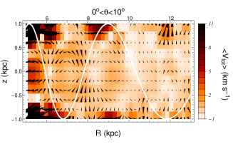
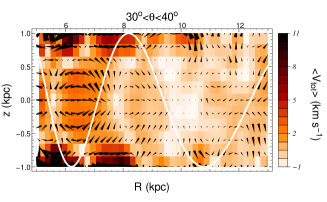
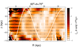
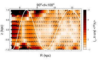
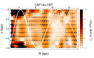
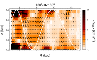
Figure 14: Same as Fig. 13, but for six different azimuths at a fixed time ($t=6\,$Gyr).

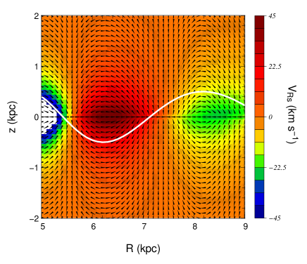
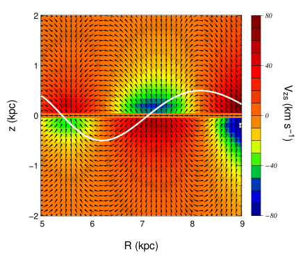
Figure 15: Analytical calculation of the response of a cold fluid to a spiral perturbation (Eq. 9) in terms of radial velocity $v_{Rs}$ (left panel) and vertical velocity $v_{zs}$ (right panel). This velocity flow is computed at $\theta=30^{\circ}$ and $t=0$ from the solution of linearized Euler equations in Eqs. 11 and 12. Arrows indicate the direction of the fluid velocity vector in the meridional plane. The white line indicates the absolute value of the spiral potential. The shape of the pattern is the same as in the simulation, and similar to Fig. 13 of Williams et al. (2013).

If we now turn our attention to the vertical motion of stars, we see on Fig. 10 that the total mean vertical motion of stars remains zero at all times, but that there is still a slight, but reasonable, vertical heating going on in the inner Galaxy.

What is most interesting is to concentrate on the mean vertical motion $\langle v_{z}\rangle$ as a function of position above or below the Galactic disc. As can be seen on Fig. 11 and Fig. 12, while the vertical velocities are generally close to zero right within the plane, they are non-zero outside of it. At a given azimuth within the frame of the spiral, these non-zero vertical velocity patterns are extremely stable over time (Fig. 11). Within corotation the mean vertical motion is directed away from the plane at the outer edge of the arm and towards the plane at the inner edge of the arm. The pattern of $\langle v_{z}\rangle$ above and below the plane are thus mirror-images, and the direction of the mean motion changes roughly in the middle of the interarm region. This produces diagonal features in terms of isocontours of a given $\langle v_{z}\rangle$, corresponding precisely to the observation using RAVE by Williams et al. (2013, see especially their Fig. 13), where the change of sign of $\langle v_{z}\rangle$ precisely occurs in between the Perseus and Scutum main arms.

Our simulation predicts that the $\langle v_{z}\rangle$ pattern is reversed outside of corotation (beyond 12 kpc), where stars move towards the plane on the outer edge of the arm (rather than moving away from the plane): this can indeed be seen, e.g., on the right panel of the second row of our Fig. 12. If we now combine the information on $\langle v_{R}\rangle$ and $\langle v_{z}\rangle$, we can plot the global meridional velocity flow $\vec{\langle v\rangle}=\langle v_{R}\rangle\vec{1}_{R}+\langle v_{z}\rangle\vec{1}_{z}$ on Fig. 13 and Fig. 14. The picture that emerges is the following: in the interarm regions located within corotation, stars move on average from the inner arm to the outer arm by going outside of the plane, and then coming back towards the plane at mid-distance between the two arms, to finally arrive back on the inner edge of the outer arm. For each azimuth, there are thus “source” points, preferentially on the outer edge of the arms (inside corotation, whilst on the inner edge outside corotation), out of which the mean velocity vector flows, while there are “sink” points, preferentially on the inner edge of the arms (inside corotation), towards which the mean velocity flows. This supports the interpretation of the observed RAVE velocity field of Williams et al. (2013) as “compression/rarefaction” waves.

3.3 Interpretation from linearized Euler equations

In order to understand these features found in the meridional velocity flow of our test-particle simulation, we now turn to the fluid approximation based on linearized Euler equations, developed, e.g., in Binney & Tremaine (2008, Sect. 6.2). A rigorous analytical treatment of a quasi-static spiral perturbation in a three-dimensional stellar disk should rely on the linearized Boltzmann equations, which we plan to do in full in a forthcoming paper, but the fluid approximation can already give important insights on the shape of the velocity flow expected in the meridional plane. In the full Boltzmann-based treatment, the velocity flow will be tempered by reduction factors both in the radial (see, e.g., Binney & Tremaine 2008, Appendix K) and vertical directions.

Let us rewrite our perturber potential of Eq. 8 as

$$\Phi_{s}=\mathbf{Re}\{\Phi_{a}(R,z)\exp[i\,m(\Omega_{P}t-\theta)]\}$$ (9)

with

$$\Phi_{a}=-A\,{\mathrm{s}ech}^{2}\left(\frac{z}{z_{0}}\right)\exp\Big{(}i\frac{m\ln(R)}{\tan p}\Big{)}.$$ (10)

Then if we write solutions to the linearized Euler equations for the response of a cold fluid as

$$\left\{\begin{array}[]{l}v_{Rs}=\mathbf{Re}\{v_{Ra}(R,z)\exp[i\,m(\Omega_{P}t-\theta)]\}\\ \\ v_{zs}=\mathbf{Re}\{v_{za}(R,z))\exp[i\,m(\Omega_{P}t-\theta)]\}\\ \end{array}\right.$$ (11)

we find, following the same steps as in Binney & Tremaine (2008, Sect. 6.2)

$$\left\{\begin{array}[]{l l}v_{Ra}=&-\frac{m(\Omega-\Omega_{P})}{\Delta}k\Phi_{a}\\ &+i\frac{2\Phi_{a}}{\Delta}\left(\frac{2\Omega{\rm tanh}(z/z_{0})}{m(\Omega-\Omega_{P})z_{0}}+\frac{m\Omega}{R}\right)\\ \\ v_{za}=&-\frac{2i}{m(\Omega-\Omega_{P})z_{0}}{\rm tanh}\Big{(}\frac{z}{z_{0}}\Big{)}\Phi_{a}\\ \end{array}\right.$$ (12)

where $k=m/(R\,{\rm tan\,}p)$ is the radial wavenumber and $\Delta=\kappa^{2}-m^{2}(\Omega-\Omega_{P})^{2}$.

If we plot these solutions for $v_{Rs}$ and $v_{zs}$ at a given angle (for instance $\theta=30^{\circ}$) we get the same pattern as in the simulation (Fig. 15). Of course, the velocity flow plotted on Fig. 15 would in fact be damped by a reduction factor depending on both radial and vertical velocity dispersions when treating the full linearized Boltzmann equation, which will be the topic of a forthcoming paper. Nevertheless, this qualitative consistency between analytical results and our simulations is an indication that the velocity pattern observed by Williams et al. (2013) is likely linked to the potential perturbation by spiral arms. Interestingly, this analytical model also predicts that the radial velocity gradient should become noticeably North/South asymmetric close to corotation.

4 Discussion and conclusions

In recent years, various large spectroscopic surveys have shown that stars of the Milky Way disc exhibit non-zero mean velocities outside of the Galactic plane in both the Galactocentric radial component and vertical component of the mean velocity field (e.g., Siebert et al. 2011b; Williams et al. 2013; Carlin et al. 2013). While it is clear that such a behaviour could be due to a large combination of factors, we investigated here whether spiral arms are able to play a role in these observed patterns. For this purpose, we investigated the orbital response of a test population of stars representative of the old thin disc to a stable spiral perturbation. This is done using a test-particle simulation with a background potential representative of the Milky Way.

We found non-zero velocities both in the Galactocentric radial and vertical velocity components. Within the rotating frame of the spiral pattern, the location of these non-zero mean velocities in both components are stable over time, meaning that the response to the spiral perturbation is stable. Within corotation, the mean $\langle v_{R}\rangle$ is negative within the arms (mean radial motion towards the Galactic centre) and positive (radial motion towards the anticentre) between the arms. Outside corotation, the pattern is reversed, as expected from the Lin-Shu density wave theory (Lin & Shu 1964). On the other hand, even though the spiral perturbation of the potential is very thin, the radial velocity flow is still strongly affected above the Galactic plane. Up to five times the scale-height of the spiral potential, there are no strong asymmetries in terms of radial velocity, but above these heights, the trend in the radial velocity flow is reversed. This means that asymmetries could be observed in surveys covering different volumes above and below the Galactic plane. Also, forthcoming surveys like Gaia, 4MOST, WEAVE will be able to map this region of the disc of the Milky Way and measure the height at which the reversal occurs. Provided this measurement is successful, it would give a measurement of the scale height of the spiral potential.

In terms of vertical velocities, within corotation, the mean vertical motion is directed away from the plane at the outer edge of the arms and towards the plane at the inner edge of the arms. The patterns of $\langle v_{z}\rangle$ above and below the plane are thus mirror-images (see e.g. Carlin et al. 2013). The direction of the mean vertical motion changes roughly in the middle of the interam region. This produces diagonal features in terms of isocontours of a given $\langle v_{z}\rangle$, as observed by Williams et al. (2013). The picture that emerges from our simulation is one of “source” points of the velocity flow in the meridional plane, preferentially on the outer edge of the arms (inside corotation, whilst on the inner edge outside corotation), and of “sink” points, preferentially on the inner edge of the arms (inside corotation), towards which the mean velocity flows.

We have then shown that this qualitative structure of the mean velocity field is also the behaviour of the analytic solution to linearized Euler equations for a toy model of a cold fluid in response to a spiral perturbation. In a more realistic analytic model, this fluid velocity would in fact be damped by a reduction factor depending on both radial and vertical velocity dispersions when treating the full linearized Boltzmann equation.

In a next step, the features found in the present test-particle simulations will also be checked for in fully self-consistent simulations with transient spiral arms, to check whether non-zero mean vertical motions as found here are indeed generic. The response of the gravitational potential itself to these non-zero motions should also have an influence on the long-term evolution of the velocity patterns found here, in the form of e.g. bending and corrugation waves. The effects of multiple spiral patterns (e.g., Quillen et al. 2011) and of the bar (e.g., Monari et al. 2013, 2014) should also have an influence on the global velocity fiel and on its amplitude. Once all these different dynamical effects and their combination will be fully understood, a full quantitative comparison with present and future datasets in 3D will be the next step.

The present work on the orbital response of the thin disc to a small spiral perturbation by no means implies that no external perturbation of the Milky Way disc happened in the recent past, by e.g. the Sagittarius dwarf (e.g., Gomez et al. 2013). Such a perturbation could of course be responsible for parts of the velocity structures observed in various recent large spectrosocpic surveys. For instance, concerning the important north-south asymmetry spotted in stellar densities at relatively large heights above the disc, spiral arms are less likely to play an important role. Nevertheless, any external perturbation will also excite a spiral wave, so that understanding the dynamics of spirals is also fundamental to understanding the effects of an external perturber. The qualitative similarity between our simulation (e.g., Fig. 11), as well as our analytical estimates for the fluid approximation (Fig. 15), and the velocity pattern observed by Williams et al. (2013, their Fig. 13) indicates that spiral arms are likely to play a non-negligible role in the observed velocity pattern of our “wobbly Galaxy”.

References

- (1) Antoja T., Valenzuela O., Pichardo B., et al., 2009, ApJ, 700, L78
- (2) Antoja T., Figueras F., Romero-Gómez M., et al., 2011, MNRAS, 418, 1423
- (3) Barros D., Lépine J., Junqueira T., 2013, MNRAS, 435, 2299
- (4) Bienaymé O., Séchaud N., 1997, A&A, 323, 781
- (5) Binney J., Tremaine S., 2008, Galactic Dynamics, Princeton University Press
- (6) Binney J., 2013, New Astronomy Reviews, 57, 29
- (7) Binney J., Burnett B., Kordopatis G., et al., 2013, arXiv:1309.4285
- (8) Bovy J., Allende Prieto C., Beers T., et al., 2012, ApJ, 759, 131
- (9) Bovy J., Rix H.-W., 2013, arXiv:1309.0809
- (10) Carlin J.L., DeLaunay J., Newberg H. J., et al., 2013, ApJ, 777, L5
- (11) Chereul E., Crézé M., Bienaymé O., 1998, A&A, 340,384
- (12) Chereul E., Crézé M., Bienaymé O., 1999, A&AS, 135, 5
- (13) Dehnen W., 1998, AJ, 115, 2384
- (14) Dehnen W., Binney J., 1998, MNRAS, 294, 429
- (15) Dehnen W., 2000, AJ, 119, 800
- (16) De Simone R., Wu X., Tremaine S., 2004, MNRAS, 350, 627
- (17) Famaey B., Jorissen A., Luri X., et al., 2005, A&A, 430, 165
- (18) Famaey B., Pont F., Luri X., et al., 2007, A&A 461, 957
- (19) Famaey B., Siebert A., Jorissen A., 2008, A&A, 483, 453
- (20) Feldmann R., Spolyar D., 2013, arXiv:1310.2243
- (21) Gomez F., Minchev I., O’Shea B., et al., 2013, MNRAS, 429, 159
- (22) Kaasalainen M., Binney J., 1994, MNRAS, 268, 1033
- (23) Kaasalainen M., 1994, MNRAS, 268, 1041
- (24) Kaasalainen M., 1995, Phys. Rev. E, 52, 1193
- (25) Kordopatis G., Gilmore G., Steinmetz M., et al., 2013, 146, 134
- (26) Kuijken K., Tremaine S., 1994, ApJ, 421, 178
- (27) Lépine J., Cruz P., Scarano S., et al., 2011, MNRAS, 417, 698
- (28) Lin C.C., Shu F.H., 1964, ApJ, 140, 646
- (29) McMillan P.J., Binney J., 2010, MNRAS, 402, 934
- (30) McMillan P.J., 2013, MNRAS, 430, 3276
- (31) Minchev I., Nordhaus J., Quillen A., 2007, ApJ, 664, L31
- (32) Minchev I., Famaey B., 2010, ApJ, 722, 112
- (33) Minchev I., Boily C., Siebert A., Bienaymé O., 2010, MNRAS, 407, 2122
- (34) Minchev I., Famaey B., Quillen A., et al., 2012, A&A, 548, A126
- (35) Monari G., Antoja T., Helmi A., 2013, arXiv:1306.2632
- (36) Monari G., Helmi A., Antoja T., Steinmetz M., 2014, arXiv:1402.4479
- (37) Olling R., Dehnen W., 2003, ApJ, 599, 275
- (38) Patsis P.A., Grosbøl P., 1996, A&A, 315, 371
- (39) Pompéia L., Masseron T., Famaey B., et al., 2011, MNRAS, 415, 1138
- (40) Quillen A., Minchev I., 2005, AJ, 130, 576
- (41) Quillen A., Dougherty J., Bagley M., et al., 2011, MNRAS, 417, 762
- (42) Reid M., Menten K., Zheng X., et al. 2009, ApJ, 700, 137
- (43) Roskar R., Debattista V., Quinn T., Wadsley J., 2012, MNRAS, 426, 2089
- (44) Schönrich R., 2012, MNRAS, 427, 274
- (45) Sellwood J., 2013, Rev. Mod. Phys., arXiv:1310.0403
- (46) Shu F.H., 1969, ApJ, 158, 505
- (47) Siebert A., Williams M.E.K., Siviero A., et al., 2011a, AJ, 141, 187
- (48) Siebert A., Famaey B., Minchev I., et al., 2011b, MNRAS, 412, 2026
- (49) Siebert A., Famaey B., Binney J., et al., 2012, MNRAS, 425, 2335
- (50) Smith M., Whiteoak S. H., Evans N. W., 2012, ApJ, 746, 181
- (51) Steinmetz M., Zwitter T., Siebert A., et al., 2006, AJ, 132, 1645
- (52) Widrow L., Gardner S., Yanny B., et al., 2012, ApJ, 750, L41
- (53) Williams M., Steinmetz M., Binney J., et al., 2013, MNRAS, 436, 101
- (54) Yanny B., Gardner S., 2013, ApJ, 777, 91
- (55) Zwitter T., Siebert A., Munari U., et al., 2008, AJ, 136, 421