Numerical methods for one-dimensional aggregation equations

Abstract

We focus in this work on the numerical discretization of the one dimensional aggregation equation $\partial_{t}\rho+\partial_{x}(v\rho)=0$, $v=a(W^{\prime}*\rho)$, in the attractive case. Finite time blow up of smooth initial data occurs for potential $W$ having a Lipschitz singularity at the origin. A numerical discretization is proposed for which the convergence towards duality solutions of the aggregation equation is proved. It relies on a careful choice of the discretized macroscopic velocity $v$ in order to give a sense to the product $v\rho$. Moreover, using the same idea, we propose an asymptotic preserving scheme for a kinetic system in hyperbolic scaling converging towards the aggregation equation in hydrodynamical limit. Finally numerical simulations are provided to illustrate the results.

Keywords.  aggregation equation, duality solutions, finite volume schemes, asymptotic preserving schemes, weak measure solutions, hydrodynamical limit.

2010 AMS classifications.  35B40, 35D30, 35L60, 35Q92, 65M08.

1 Introduction

This paper is devoted to the numerical approximation of the so-called aggregation equation which writes in one space dimension

$$\partial_{t}\rho+\partial_{x}\big{(}a(W^{\prime}*\rho)\rho\big{)}=0.$$ (1.1)

This equation is complemented with some initial data $\rho(0,x)=\rho^{ini}(x)$. This nonlocal and nonlinear conservation equation is involved in many applications in physics and biology (see e.g. [3, 11, 32, 33, 35, 31] in the case $a$ linear. It describes the behaviour of a population of particles (in physical applications) or cells (in biological applications) interacting under a continuous interaction potential $W$. The quantity $\rho$ denotes the density of these particles or cells. The function $a$ is often linear ($a(u)=\pm u$), but in several applications, such as pedestrian motion [14, 15] or chemotaxis (see [22] and Section 4.2 below) a specific nonlinearity has to be considered. Depending on the choice of the potential $W$ and the function $a$, one can be in the repulsive or in the attractive case, which leads to aggregation phenomena.

In this work we mainly focus on the case involving attractive forces. Individuals attract one another under the action of the potential $W$, assumed to be smooth away of $0$ and bounded from below. More precisely, $W$ satisfies the following properties:

Definition 1.1

We say that $W\in C^{1}(\mathbb{R}\setminus\{0\})$ is a pointy attractive potential if

$$W^{\prime\prime}=-\delta_{0}+w,\quad w\in C_{b}(\mathbb{R}),\quad\mbox{ with }\ \|w\|_{L^{1}(\mathbb{R})}=w_{0}<\infty,$$ (1.2)

in the distributional sense, where $\delta_{0}$ is the Dirac measure at $0$.

Attractivity in the nonlinear case is ensured provided the function $a$ satisfies

$$a\in C^{1}(\mathbb{R}),\qquad 0\leq a^{\prime}(x)\leq\alpha,\quad\forall\,x\in\mathbb{R}.$$ (1.3)

This case has been extensively studied in the linear case $a=\mbox{id}$ [4, 5, 6] and it is known that if the potential $W$ has a Lipschitz singularity then weak solutions blow up in finite time (see e.g. [4, 22]), so that measure valued solutions arise. At the theoretical level, global in time existence has been obtained in the linear case $a=\mbox{id}$ and in any space dimension by Carrillo et al. [13], in the space ${\mathcal{P}}_{2}$ of probability measures with finite second moment, using the geometrical approach of gradient flows. In the nonlinear case, but in one space dimension, global existence of measure solutions has been obtained by completely different means in [25], namely thanks to the notion of duality solutions. It has also been proved in [25] that in the linear case $a=\mbox{id}$, both notions coincide. The key point leading to both uniqueness of solutions and equivalence between the two notions is the definition of the macroscopic velocity. In the framework of gradient flows, it is defined as the unique element with minimal norm in the subdifferential of the interaction energy associated to $W$, where ${\mathcal{P}}_{2}$ is endowed with the Wasserstein distance (see [2, 13] for more details). In [25], the macroscopic velocity is defined using the chain rule for BV functions, and this is the viewpoint adopted for numerical analysis.

In some applications, the aggregation equation is the hydrodynamic limit of some kinetic sytem (see [16, 17, 22] for examples in chemotaxis). We consider here the following kinetic model with relaxation in hyperbolic scaling

$$\partial_{t}f_{\varepsilon}+v\partial_{x}f_{\varepsilon}=\frac{1}{\varepsilon}(\rho_{\varepsilon}E(v,W^{\prime}*\rho_{\varepsilon})-f_{\varepsilon}),$$ (1.4)

where $f_{\varepsilon}$ is the ditribution function of cells at time $t$, position $x$ and velocity $v$, $\rho_{\varepsilon}=\int f_{\varepsilon}\,dv$ and the equilibrium function $E$ is normalized so that $\int E\,dv=1$. Existence of global in time $L^{\infty}$ weak solutions for such a kinetic equation with fixed $\varepsilon>0$ is well-known (see e.g. [10, 36]). However taking the limit $\varepsilon\to 0$, we recover the aggregation equation (1.1) (see Theorem 3.1 below), for which solutions blow up in finite time. Then an interesting issue consists in providing a numerical scheme for the kinetic system (1.4) which allows to recover the asymptotic limit when $\varepsilon\to 0$. Such schemes are usually called asymptotic preserving (AP) [27]. They are of great interest for kinetic equations since letting $\varepsilon\to 0$ with the mesh size and time step fixed, the scheme becomes a scheme for the macroscopic limit (see e.g. [18, 28, 30]). In other words, AP schemes allow a numerical discretization whose time step is not constrained by some constant depending on $\varepsilon$. We refer to [26] for a review on AP schemes.

The aim of this work is precisely to design numerical methods for (1.1) and (1.4) that are able to capture the measure solutions after blow-up. The main difficulty is that after blow up the velocity $a(W^{\prime}*\rho)$ is discontinuous, so that the definition of the flux has to be considered with great care. Following the principle that holds at the continuous level, the numerical velocity is obtained thanks a careful discretization of the Vol’pert calculus for BV functions. We emphasize that the numerical solution may depend upon the way of discretizing the velocity. For equation (1.1) we work directly on the definition of $a(W^{\prime}*\rho)$, for the kinetic model, the discretization is defined through the right-hand side of equation (1.4). The final scheme is obtained by a splitting technique, as in for instance [28, 29], which is in this particular case very easy to implement. A more sophisticated technique consists in using well-balanced schemes [21] as it has been successfully used for chemotaxis models in [20, 19]. However, it is not clear that such schemes allow to recover the solutions after blow up.

The outline of the paper is as follows. Section 2 is devoted to the aggregation equation (1.1). After recalling existence and uniqueness result for this system, we provide a numerical scheme and prove its convergence. In Section 3, we consider the kinetic equation (1.4). We first establish the rigorous derivation of the aggregation equation thanks to a hyperbolic limit $\varepsilon\to 0$. Then we propose an asymptotic preserving scheme and prove its convergence. Finally, Section 4 is devoted to some numerical simulations.

Part of these results were announced in [24].

2 Aggregation equation

2.1 Existence of duality solutions

For $Y$ and $Z$ two metric spaces we denote $C_{b}(Y,Z)$ the set of continuous and bounded functions from $Y$ to $Z$, $C_{0}(Y,Z)$ the set of those that vanish at infinity and $C_{c}(Y,Z)$ the set of continuous functions with compact support. Let ${\cal M}_{b}(\mathbb{R})$ be the set of bounded Radon measures and by ${\cal P}_{1}(\mathbb{R})$ the set of positive measure in ${\cal M}_{b}(\mathbb{R})$ such that $\int_{\mathbb{R}}|x|d\mu(x)<\infty$. From now on, the space ${\cal M}_{b}(\mathbb{R}^{N})$ is always endowed with the weak topology $\sigma({\cal M}_{b},C_{0})$. We denote ${\cal S}_{\cal M}:=C([0,T];{\cal M}_{b}(\mathbb{R}^{N})-\sigma({\cal M}_{b},C_{0}))$.

Duality solutions have been introduced in [8] to solve scalar conservation laws with discontinuous coefficients. More precisely, it gives sense to measure valued solutions of the scalar conservation law

$$\partial_{t}\rho(t,x)+\partial_{x}(b(t,x)\rho(t,x))=0,$$

where $b\in L^{\infty}((0,T)\times\mathbb{R})$ satisfies the so-called one-sided Lipschitz condition

$$\partial_{x}b(t,.)\leq\beta(t)\qquad\mbox{for $\beta\in L^{1}(0,T)$, in the distributional sense}.$$ (2.1)

This key point suggests that the velocity field should be compressive. We refer to [8] for the precise definition and general properties of these solutions.

Let us first define a notion of duality solution for the aggreagation equation (1.1) in the spirit of [9, 23]:

Definition 2.1

We say that $\rho\in C([0,T];{\cal M}_{b}(\mathbb{R}))$ is a duality solution to (1.1) if there exists $\widehat{a}_{\rho}\in L^{\infty}((0,T)\times\mathbb{R})$ and $\alpha\in L^{1}_{loc}(0,T)$ satisfying $\partial_{x}\widehat{a}_{\rho}\leq\alpha$ in ${\cal D}^{\prime}((0,T)\times\mathbb{R})$, such that for all $0<t_{1}<t_{2}<T$,

$$\partial_{t}\rho+\partial_{x}(\widehat{a}_{\rho}\rho)=0\qquad\mbox{in the sense of duality on }(t_{1},t_{2}),$$

and $\widehat{a}_{\rho}=a(W^{\prime}*\rho)$ a.e.

From now on, we denote by $A$ the antiderivative of $a$ such that $A(0)=0$. Using the chain rule, a natural definition of the flux is

$$J:=-\partial_{x}A(W^{\prime}*\rho)+a(W^{\prime}*\rho)w*\rho.$$ (2.2)

In fact, a formal computation shows that

$$-\partial_{x}A(W^{\prime}*\rho)=-a(W^{\prime}*\rho)W^{\prime\prime}*\rho=a(W^{\prime}*\rho)(\rho-w*\rho),$$

where we use (1.2) for the last identity.

Then we are in position to state the existence and uniqueness result of [25].

Theorem 2.2 ([25], Theorem 3.9)

Let us assume that $\rho^{ini}$ is given in ${\cal P}_{1}(\mathbb{R})$. Under Assumptions 1.1 on the potential $W$ and (1.3) for the nonlinear function $a$, for all $T>0$ there exists a unique duality solution $\rho$ of (1.1) in the sense of Definition 2.1 with $\rho\geq 0$, $\rho(t)\in{\cal P}_{1}(\mathbb{R})$ for $t\in(0,T)$ and which satisfies in the distributional sense:

$$\partial_{t}\rho+\partial_{x}J=0,$$ (2.3)

where $J$ is defined in (2.2). Moreover, there exists $\widehat{a}$, called universal representative, such that $\widehat{a}=a(W^{\prime}*\rho)$ a.e. Then $\rho=X_{\#}\rho^{ini}$, where $X$ is the Filippov flow associated to the velocity $\widehat{a}$.

2.2 Numerical discretization

Let us consider a uniform space discretization with step $\delta x$ and denote by $\delta t$ the time step; then $t_{n}=n\delta t$ and $x_{i}=x_{0}+i\delta x$, $i=0,\ldots,N_{x}$. We assume that the initial datum $\rho^{ini}$ is compactly supported with support included in $[x_{0},x_{N_{x}}]$, and since this work is not concerned with boundary conditions, we assume as well that the solutions are compactly supported in the computational domain during the computational time. Then from now on, we take $\rho_{0}^{n}=S_{0}^{n}=S_{1}^{n}=J_{-1/2}^{n}=0$ and $\rho_{N_{x}}^{n}=S_{N_{x}}^{n}=J_{N_{x}+1/2}^{n}=0$.

For $n\in\mathbb{N}$, we assume to have computed an approximation $(\rho_{i}^{n})_{i=0,\ldots,N_{x}}$ of $(\rho(t_{n},x_{i}))_{i=0,\ldots,N_{x}}$, we denote by $(S_{i}^{n})_{i=0,\ldots,N_{x}}$ an approximation of $(W*\rho(t_{n},x_{i}))_{i=0,\ldots,N_{x}}$ and by $(\nu_{i}^{n})_{i=0,\ldots,N_{x}}$ an approximation of $(w*\rho(t_{n},x_{i}))_{i=0,\ldots,N_{x}}$. Let us denote $\lambda=\delta t/\delta x$ and $M$ the total mass of the system, $M=|\rho^{ini}|(\mathbb{R})$. We obtain an approximation of $\rho(t_{n+1},x_{i})$ denoted $\rho_{i}^{n+1}$ by using the following Lax-Friedrichs discretization of equation (2.3)–(2.2):

$$\rho_{i}^{n+1}=\rho_{i}^{n}-\frac{\lambda}{2}(J_{i+1/2}^{n}-J_{i-1/2}^{n})+\frac{\lambda}{2}c(\rho_{i+1}^{n}-2\rho_{i}^{n}+\rho_{i+1}^{n})$$ (2.4)

$$J_{i+1/2}^{n}=-\frac{A(\partial_{x}S_{i+1}^{n})-A(\partial_{x}S_{i}^{n})}{\delta x}+a_{i+1/2}^{n}\frac{\nu_{i+1}^{n}+\nu_{i}^{n}}{2},$$ (2.5)

where we have defined

$$c:=\max_{x\in[-M(1+w_{0}),M(1+w_{0})]}|a(x)|.$$ (2.6)

In this scheme, we use the discretization

$$\partial_{x}S_{i+1}^{n}=\frac{S_{i+2}^{n}-S_{i}^{n}}{2\delta x},$$ (2.7)

and the approximation

$$a_{i+1/2}^{n}=\left\{\begin{array}[]{ll}0&\mbox{ if }\ \partial_{x}S_{i+1}^{n}=\partial_{x}S_{i}^{n},\\[5.69054pt] \displaystyle\frac{A(\partial_{x}S_{i+1}^{n})-A(\partial_{x}S_{i}^{n})}{\partial_{x}S_{i+1}^{n}-\partial_{x}S_{i}^{n}}&\mbox{ otherwise.}\end{array}\right.$$ (2.8)

We need now a scheme for $S_{i}^{n}$. From Assumption 1.1, we deduce by taking the convolution of (1.2) with $\rho$ that $-W^{\prime\prime}*\rho+w*\rho=\rho$. This equation is discretized by using a standard finite difference scheme:

$$-\frac{S_{i+1}^{n}-2S_{i}^{n}+S_{i-1}^{n}}{\delta x^{2}}+\nu_{i}^{n}=\rho_{i}^{n}.$$ (2.9)

This scheme allows the computation of $(S_{i}^{n})_{i}$, provided $(\nu_{i}^{n})_{i}$ is known. For the computation of $(\nu_{i}^{n})_{i}$, there are multiple ways; here we propose to use a piecewise constant approximation for $\rho$ on each interval $[x_{i},x_{i+1})$, so that

$$\nu_{i}^{n}=\sum_{k=1}^{N_{x}}\int_{x_{k}}^{x_{k+1}}\rho_{i}^{n}w(x_{i}-y)\,dy,$$

which can be rewritten

$$\nu_{i}^{n}=\sum_{k=1}^{N_{x}}\rho_{k}^{n}w_{ki},\quad w_{ki}=\int_{x_{i}-x_{k+1}}^{x_{i}-x_{k}}w(z)\,dz=\int_{(i-1-k)\delta x}^{(i-k)\delta x}w(z)\,dz.$$ (2.10)

Now the final version of the scheme for $\rho_{i}^{n}$ can be written. Using (2.7) and (2.9), we deduce that we can rewrite (2.5) as

$$J_{i+1/2}^{n}=a_{i+1/2}^{n}\frac{\rho_{i+1}^{n}+\rho_{i}^{n}}{2}.$$ (2.11)

Injecting this latter expression of the flux in (2.4) we obtain

$$\rho^{n+1}_{i}=\rho_{i}^{n}\big{(}1-\lambda c+\frac{\lambda}{4}(a_{i-1/2}^{n}-a_{i+1/2}^{n})\big{)}+\frac{\lambda}{2}\left(c+\frac{a_{i-1/2}^{n}}{2}\right)\rho_{i-1}^{n}+\frac{\lambda}{2}\left(c-\frac{a_{i+1/2}^{n}}{2}\right)\rho_{i+1}^{n}.$$ (2.12)

We emphasize at this point the importance of the choice of the discretization of the macroscopic velocity $a_{i+1/2}^{n}$ in (2.8) as it is the one corresponding to the universal representative $\widehat{a}$ of Theorem 2.2. Numerical example showing a wrong dynamics with a different discretization choice will be provided in Section 4.2.

Remark 2.3

The choice of the discretization (2.8) for the macroscopic velocity can be seen as a consequence of the chain rule (or Vol’pert calculus) for $BV$ functions [37] (see also remark 3.98 of [1]): for a BV function $u$, the fonction $\widehat{a}_{V}$ defining the chain rule $\partial_{x}A(u)=\widehat{a}_{V}\partial_{x}u$ is constructed by

$$\widehat{a}_{V}(x)=\int_{0}^{1}a(tu_{1}(x)+(1-t)u_{2}(x))\,dt,$$ (2.13)

where

$$(u_{1},u_{2})=\left\{\begin{array}[]{ll}\displaystyle(u,u)&\qquad\mbox{ if }x\in\mathbb{R}\setminus S_{u},\\[5.69054pt] \displaystyle(u^{+},u^{-})&\qquad\mbox{ if }x\in J_{u},\\[5.69054pt] \displaystyle\mbox{ arbitrary }&\qquad\mbox{elsewhere.}\end{array}\right.$$ (2.14)

We have denoted by $S_{u}$ the set of $x\in\mathbb{R}$ where $u$ does not admit an approximate limit and by $J_{u}\subset S_{u}$ the set of jump points. Applying that to $u=\partial_{x}S$, we obtain,

$$\widehat{a}_{V}(x)=\left\{\begin{array}[]{ll}\displaystyle a(\partial_{x}S(x))&\mbox{ if }x\in\mathbb{R}\setminus S_{u},\\[5.69054pt] \displaystyle\frac{A(\partial_{x}S(x^{+}))-A(\partial_{x}S(x^{-}))}{\partial_{x}S(x^{+})-\partial_{x}S(x^{-})}&\mbox{ if }x\in J_{u},\\[8.53581pt] \displaystyle\mbox{ arbitrary }&\mbox{elsewhere.}\end{array}\right.$$ (2.15)

2.3 Numerical analysis

In this subsection, we prove the convergence of the numerical scheme defined in (2.4)–(2.8) towards the unique duality solution of Theorem 2.2. We first state a Lemma which proves a CFL-like condition for the scheme:

Lemma 2.4

Let us assume that (1.3) holds and that the condition

$$\lambda:=\frac{\delta t}{\delta x}\leq\frac{2}{3c},$$ (2.16)

is satisfied with $c$ defined in (2.6). Let us assume that $\rho^{ini}\in{\cal P}_{1}(\mathbb{R})$ is given, compactly supported and nonnegative, and we define $\rho_{i}^{0}=\frac{1}{\delta x}\int_{x_{i}}^{x_{i+1}}\rho^{ini}(dx)\geq 0$.

Then for all $i$ and $n\in\mathbb{N}$, the sequences computed thanks to the scheme defined in (2.4)–(2.9) satisfy

$$\rho_{i}^{n}\geq 0,\qquad|a_{i+1/2}^{n}|\leq c.$$

Proof.

We choose $x_{0}$ and $x_{N_{x}}$ such that supp$(\rho^{ini})\subset[x_{0},x_{N_{x}}]$. Let us define $M_{i}^{n}=\delta x\sum_{j=0}^{i}\rho_{j}^{n}$ and $M^{n+1}_{i}=\delta x\sum_{j=0}^{i}\rho^{n+1}_{j}$. Since the scheme (2.4) is conservative, we have $M_{N_{x}}^{n}=M_{N_{x}}^{0}=M$. Clearly, $\rho_{i}^{n}=(M_{i}^{n}-M_{i-1}^{n})/\delta x$ and from (2.11) we have $J_{i+1/2}^{n}=a_{i+1/2}^{n}(M_{i+1}^{n}-M_{i-1}^{n})/(2\delta x)$. Then we deduce from (2.4) that

$$M_{i}^{n+1}=(1-\lambda c)M_{i}^{n}+\frac{\lambda}{2}\left(c-\frac{a_{i+1/2}^{n}}{2}\right)M_{i-1}^{n}+\frac{\lambda}{2}\left(c+\frac{a_{i+1/2}^{n}}{2}\right)M_{i+1}^{n}.$$ (2.17)

By definition of $\nu_{i}^{n}$ in (2.10), we deduce from (1.2) that for all $i\in\mathbb{N}^{*}$,

$$\delta x\sum_{j=1}^{i}\big{|}\nu_{j}^{n}\big{|}\leq\delta x\sum_{k=1}^{N_{x}}\rho_{k}^{n}w_{0}=Mw_{0}.$$ (2.18)

Moreover, from the definition of $\partial_{x}S_{i}^{n}$ in (2.7) and using equation (2.9), we deduce

$$-\frac{\partial_{x}S_{i+1}^{n}-\partial_{x}S_{i}^{n}}{\delta x}+\frac{\nu_{i+1}^{n}+\nu_{i}^{n}}{2}=\frac{\rho_{i+1}^{n}+\rho_{i}^{n}}{2}.$$

Summing this latter equation over $i$, we obtain

$$\partial_{x}S_{i+1}^{n}=\partial_{x}S_{0}^{n}+\frac{1}{2}\big{(}-M_{i+1}^{n}-M_{i}^{n}+M_{0}^{n}+\delta x\big{(}2\sum_{j=0}^{i}\nu_{j}^{n}+\nu_{i+1}^{n}-\nu_{0}^{n}\big{)}\big{)}.$$

Using the boundary conditions, we have $\partial_{x}S_{0}^{n}=0$ and $M_{0}^{n}=0$. Then,

$$\partial_{x}S_{i+1}^{n}=-\frac{1}{2}\big{(}M_{i+1}^{n}+M_{i}^{n}-\delta x\big{(}2\sum_{j=0}^{i}\nu_{j}^{n}+\nu_{i+1}^{n}-\nu_{0}^{n}\big{)}\big{)}.$$ (2.19)

We are now in position to prove the lemma by an induction on $n$. For $n=0$, by construction of the initial data, we have $\rho_{i}^{0}\geq 0$. Then for all $i$, we have $0\leq M_{i}^{0}\leq M$ and with (2.19) and (2.18) we deduce that

$$|\partial_{x}S_{i+1}^{0}|\leq M(1+w_{0}),\quad\mbox{ for all }i.$$

Futhermore, since we have

$$\frac{A(\partial_{x}S_{i+1}^{0})-A(\partial_{x}S_{i}^{0})}{\partial_{x}S_{i+1}^{0}-\partial_{x}S_{i}^{0}}=a(\theta_{i}^{0}),\qquad\theta_{i}^{0}\in(\partial_{x}S_{i}^{0},\partial_{x}S_{i+1}^{0})\subset(-M(1+w_{0}),M(1+w_{0})),$$

we deduce with (2.8) that $|a_{i+1/2}^{0}|\leq c$, which proves the result for $n=0$.

Let us assume that $\rho_{i}^{n}\geq 0$ and $|a_{i+1/2}^{n}|\leq c$, for some $n\in\mathbb{N}$. From condition (2.16) and the induction assumption $|a_{i+1/2}^{n}|\leq c$, we deduce that in the scheme (2.12), all the coefficients in front of $\rho_{i-1}^{n}$, $\rho_{i}^{n}$ and $\rho_{i+1}^{n}$ are nonnegative. Thus $\rho_{i}^{n+1}\geq 0$ for all $i$. Moreover, we have clearly by definition that $0\leq M_{i}^{n}\leq M$. Then, from the condition (2.16) and induction assumption $|a_{i+1/2}^{n}|\leq c$, we deduce with (2.17) that $M^{n+1}_{i}$ is a convex combination of $M^{n}_{i+1}$, $M_{i}^{n}$ and $M_{i-1}^{n}$. Then $0\leq M_{i}^{n+1}\leq M$. Thus, as above, using (2.19) with $n+1$ instead of $n$, we have $|\partial_{x}S_{i+1}^{n+1}|\leq M(1+w_{0})$, which implies $|a_{i+1/2}^{n+1}|\leq c$.

Let us define the reconstruction

$$\rho_{\delta}(t,x)=\sum_{n\in\mathbb{N}}\sum_{i=0}^{N_{x}}\rho_{i}^{n}{\bf 1}_{[n\delta t,(n+1)\delta t)\times[x_{i},x_{i+1})}(t,x),$$

and $S_{\delta}$, $\partial_{x}S_{\delta}$, $\nu_{\delta}$, $J_{\delta}$ and $a_{\delta}$ are defined in a similar way thanks to $(S_{i}^{n})_{i}$, $(\partial_{x}S_{i}^{n})_{i}$, $(\nu_{i}^{n})_{i}$, $(J_{i+1/2}^{n})_{i}$ and $(a_{i+1/2}^{n})_{i}$ respectively. Then we have the following convergence result:

Theorem 2.5

Let us assume that $\rho^{ini}\in{\cal P}_{1}(\mathbb{R})$ is given, compactly supported and nonnegative and define $\rho_{i}^{0}=\frac{1}{\delta x}\int_{x_{i}}^{x_{i+1}}\rho^{ini}(dx)\geq 0$. Under assumption (1.3), if (2.16) is satisfied, then the discretization $\rho_{\delta}$ converges in ${\cal S}_{\cal M}$ towards the unique duality solution $\rho$ of Theorem 2.2 as $\delta t$ and $\delta x$ go to $0$.

Proof.

As above, we assume that supp$(\rho^{ini})\subset[x_{0},x_{N_{x}}]$. Applying Lemma 2.4, we have that $(\rho_{i}^{n})_{i}$ is nonnegative and $|a_{i+1/2}^{n}|\leq c$, provided (2.16) is satisfied. As in the proof of Lemma 2.4, we define $M_{i}^{n}=\delta x\sum_{j=0}^{i}\rho_{j}^{n}$, which satisfies (2.17) and $0\leq M_{i}^{n}\leq M$. Moreover, we clearly have that $0\leq\rho_{i}^{n}=(M_{i}^{n}-M_{i-1}^{n})/\delta x$, then equation (2.12) implies a $BV(\mathbb{R})$ estimate on $(M_{i}^{n})_{i}$, provided (2.16) is satisfied. More precisely the scheme is TVD for the sequence $(M_{i}^{n})_{i}$.

Defining

$$M_{\delta}(t,x)=\sum_{n\in\mathbb{N}}\sum_{i=0}^{N_{x}}M_{i}^{n}{\bf 1}_{[n\delta t,(n+1)\delta t)\times[x_{i},x_{i+1})}(t,x),$$

we deduce from standard techniques that we have a $L^{\infty}\cap BV((0,T)\times\mathbb{R})$ estimate on $M_{\delta}$. It implies the convergence, up to a subsequence, of $M_{\delta}$ in $L^{1}_{loc}(\mathbb{R}^{+}\times\mathbb{R})$ towards a function $\widetilde{M}\in L^{\infty}\cap BV((0,T)\times\mathbb{R})$ when $\delta t$ and $\delta x$ go to $0$ and satisfy (2.16).

Let us define $\rho=\partial_{x}\widetilde{M}\in L^{\infty}((0,T);{\cal M}_{b}(\mathbb{R}))$. Obviously, noting that $\rho_{i}^{n}=(M_{i}^{n}-M_{i-1}^{n})/\delta x$, we deduce that $\rho$ is the limit in ${\cal S}_{\cal M}$ of $\rho_{\delta}$. By definition (2.10), we have that $\nu_{\delta}=w*\rho_{\delta}$. Therefore, the sequence $(\nu_{\delta})_{\delta}$ converges, up to a subsequence, towards $\nu:=w*\rho$ for a.e. $t>0$ and $x\in\mathbb{R}$.

From (2.19), we deduce that we have the same bound on the sequence $(\partial_{x}S_{i}^{n})_{i,n}$ as on $(M_{i}^{n})_{i,n}$. We conclude that the sequence $(\partial_{x}S_{i}^{n})_{i,n}$ is bounded in $L^{\infty}\cap BV((0,T)\times\mathbb{R})$. As above, we get the convergence, up to a subsequence, in $L^{1}_{loc}(\mathbb{R}^{+}\times\mathbb{R})$ of $\partial_{x}S_{\delta}$ towards a function $\partial_{x}S$ belonging to $L^{\infty}\cap BV((0,T)\times\mathbb{R})$ as $\delta t$ and $\delta x$ go to $0$ and satisfy (2.16). By definition of $\partial_{x}S_{\delta}$, we have the strong convergence up to a subsequence in $L^{1}_{loc}(\mathbb{R}^{+},W^{1,1}_{loc}(\mathbb{R}))$ of $S_{\delta}$ towards $S$.

Passing to the limit in the equation (2.9) we deduce that $S$ and $w$ satisfy in the weak sense the equation

$$-\partial_{xx}S+w=\rho.$$

Moreover, from Lemma 2.4, we deduce that the sequence $(a_{\delta})_{\delta}$ is bounded in $L^{\infty}$, thus we can extract a subsequence converging in $L^{\infty}-weak^{*}$ towards $\widetilde{a}$. From the $L^{1}_{loc}$ convergence of $(\partial_{x}S_{\delta})_{\delta}$, we deduce that $\widetilde{a}=a(\partial_{x}S)$ a.e. Then, from (2.5), we have the convergence in the sense of distribution of $J_{\delta}$ towards $J=-\partial_{x}(A(\partial_{x}S))+\widetilde{a}w$ a.e. Finally, taking the limit in the distributional sense of equation (2.4) we deduce that $\rho$ is a solution in the sense of distribution of (2.3)–(2.2). By uniqueness of this solution, we deduce that $\rho$ is the unique duality solution of Theorem 2.2.

Finally, we notice that, as in the continuous case (see [23]), the nonnegativity of the density $\rho$ allows to ensure an OSL condition on the discretized macroscopic velocity.

Proposition 2.6

With the same notations and assumptions as in Theorem 2.5, the discrete macroscopic velocity in (2.8) satisfies the discrete OSL condition:

$$\frac{1}{\delta x}\big{(}a_{i+1/2}^{n}-a_{i-1/2}^{n}\big{)}\leq C\alpha.$$

Proof.

From definition (2.8) we have, applying the mean value Theorem:

$$\frac{1}{\delta x}\big{(}a_{i+1/2}^{n}-a_{i-1/2}^{n}\big{)}=\frac{1}{\delta x}\big{(}a(\theta_{i+1/2}^{n})-a(\theta_{i-1/2}^{n})\big{)}=\frac{a^{\prime}(\gamma_{i}^{n})}{\delta x}\big{(}\theta_{i+1/2}^{n}-\theta_{i-1/2}^{n}\big{)},$$

where $\theta_{i+1/2}^{n}\in(\partial_{x}S_{i}^{n},\partial_{x}S_{i+1}^{n})$ and $\gamma_{i}^{n}\in(\theta_{i-1/2}^{n},\theta_{i+1/2}^{n})$ (where the interval $(\alpha,\beta)$ is the interval $(\beta,\alpha)$ when $\beta<\alpha$). Then, using assumption (1.3),

$$\frac{1}{\delta x}\big{(}a_{i+1/2}^{n}-a_{i-1/2}^{n}\big{)}\leq\frac{a^{\prime}(\gamma_{i}^{n})}{\delta x}\max\big{\{}0,\partial_{x}S_{i+1}^{n}-\partial_{x}S_{i}^{n},\partial_{x}S_{i}^{n}-\partial_{x}S_{i-1}^{n},\partial_{x}S_{i+1}^{n}-\partial_{x}S_{i-1}^{n}\big{\}}.$$

From the definition (2.7) and with (2.9), we have

$$\frac{\partial_{x}S_{i+1}^{n}-\partial_{x}S_{i}^{n}}{\delta x}=\frac{\nu_{i+2}^{n}+\nu_{i}^{n}}{2}-\frac{\rho_{i+1}^{n}+\rho_{i}^{n}}{2}\leq\frac{\nu_{i+2}^{n}+\nu_{i}^{n}}{2},$$

and

$$\frac{\partial_{x}S_{i+1}^{n}-\partial_{x}S_{i-1}^{n}}{\delta x}=\frac{\nu_{i+2}^{n}+2\nu_{i}^{n}+\nu_{i-1}^{n}}{2}-\frac{\rho_{i+1}^{n}+2\rho_{i}^{n}+\rho_{i-1}^{n}}{2}\leq\frac{\nu_{i+2}^{n}+2\nu_{i}^{n}+\nu_{i-1}^{n}}{2},$$

where we use the nonnegativity on the sequence $(\rho_{i}^{n})_{i,n}$. Since the sequence $(\nu_{i}^{n})_{i,n}$ is bounded in $L^{\infty}$, we deduce that $\partial_{x}S_{i+1}^{n}-\partial_{x}S_{i}^{n}$ and $\partial_{x}S_{i+1}^{n}-\partial_{x}S_{i-1}^{n}$ are bounded from above by a nonnegative constant $C$ only depending on the initial data. Using moreover assumption (1.3) allows to conclude the proof.

Remark 2.7

In applications, we can have $w=W$. In this case, we prefer to set $\nu_{i}^{n}=S_{i}^{n}$ instead of (2.10). And the sequence $(S_{i}^{n})_{i,n}$ is then entirely determined by solving system (2.9). Then it is straightforward to adapt the proof of Theorem 2.5; the convergence result still holds in this case.

3 Asymptotic preserving scheme

In this section, we consider an asymptotic preserving scheme allowing to recover the numerical discretization (2.4)–(2.5) from a kinetic model (1.4).

Asymptotic preserving (AP) schemes has been widely developed since the 90s for a wide range of time-dependent kinetic and hyperbolic equations. The basic idea is to develop a numerical discretization that preserves the asymptotic limits from the microscopic to the macroscopic models [26]. Moreover, in the definition of [27], an AP scheme should be implemented explicitely (or at least more efficiently than using a Newton type solvers for nonlinear algebraic systems).

3.1 Hydrodynamical limit

As already mentioned, aggregation equation (1.1) can be derived by a hydrodynamical limit of some kinetic equation. Here we assume that the kinetic system leading to (1.1) in hyperbolic scaling is given by the following relaxation model of BGK type

$$\partial_{t}f_{\varepsilon}+v\partial_{x}f_{\varepsilon}=\frac{1}{\varepsilon}\big{(}\rho_{\varepsilon}E(v,W^{\prime}*\rho_{\varepsilon})-f_{\varepsilon}\big{)},\qquad t\geq 0,\ x\in\mathbb{R},\ v\in V,$$ (3.1)

where we assume that the equilibrium function $E\geq 0$, $E\in C^{2}(V\times\mathbb{R})$ is normalized such that

$$\int_{V}E(v,x)\,dv=1,\quad\forall\,x\in\mathbb{R}.$$ (3.2)

Moreover we assume that the domain $V$ is a bounded interval of $\mathbb{R}$, for the clarity of the notations, we will set $V=[-V_{M},V_{M}]$. We denote by $S_{\varepsilon}$ the potential $S_{\varepsilon}=W*\rho_{\varepsilon}$, which, due to (1.2) is a weak solution to

$$-\partial_{xx}S_{\varepsilon}+w*\rho_{\varepsilon}=\rho_{\varepsilon}.$$ (3.3)

We define moreover the antiderivative

$${\cal E}(v,x)=\int^{x}_{0}E(v,y)\,dy,$$

so that

$$\partial_{xx}S_{\varepsilon}\,E(v,\partial_{x}S_{\varepsilon})=\partial_{x}{\cal E}(v,\partial_{x}S_{\varepsilon}).$$

Then we deduce formally from (3.3) that

$$\displaystyle\Pi_{\varepsilon}:=\rho_{\varepsilon}E(v,\partial_{x}S_{\varepsilon})=-\partial_{x}{\cal E}(v,\partial_{x}S_{\varepsilon})+(w*\rho_{\varepsilon})E(v,\partial_{x}S_{\varepsilon}).$$ (3.4)

Then the momentum equations resulting from this system are given by

$$\partial_{t}\rho_{\varepsilon}+\partial_{x}J_{\varepsilon}=0,$$ (3.5)

$$\partial_{t}J_{\varepsilon}+\partial_{x}q_{\varepsilon}=\frac{1}{\varepsilon}\Big{(}\int_{V}v\Pi_{\varepsilon}(v)\,dv-J_{\varepsilon}\Big{)},$$ (3.6)

where $\rho_{\varepsilon}=\int_{V}f_{\varepsilon}(x,v)\,dv$, $J_{\varepsilon}=\int_{V}vf_{\varepsilon}(x,v)\,dv$ and $q_{\varepsilon}=\int_{V}v^{2}f_{\varepsilon}(x,v)\,dv$. We define

$$a(x)=\int_{V}vE(v,x)\,dv\ ,\quad\mbox{ and }\quad A(x)=\int_{V}v{\cal E}(v,x)\,dv.$$ (3.7)

Obviously, we have $A^{\prime}=a$. Then, with this notation, we have

$$\int_{V}v\Pi_{\varepsilon}(v)\,dv=a(\partial_{x}S_{\varepsilon})\rho_{\varepsilon}=-\partial_{x}A(\partial_{x}S_{\varepsilon})+(w*\rho_{\varepsilon})a(\partial_{x}S_{\varepsilon}).$$

Letting formally $\varepsilon\to 0$ in (3.6), we get

$$J_{\varepsilon}\to J_{0}:=\int_{V}v\Pi_{0}(v)\,dv=-\partial_{x}A(\partial_{x}S_{0})+(w*\rho_{0})a(\partial_{x}S_{0}).$$

Injecting in (3.5), we recover the aggregation equation

$$\partial_{t}\rho_{0}+\partial_{x}J_{0}=0,\qquad J_{0}=-\partial_{x}A(\partial_{x}S_{0})+(w*\rho_{0})a(\partial_{x}S_{0}),$$ (3.8)

where $S_{0}=W*\rho_{0}$.

We can now establish the rigorous derivation of the macroscopic model. This is an extension of the hydrodynamical limit stated in Theorem 3.10 of [23], where a particular case appearing in bacterial chemotaxis is considered.

Theorem 3.1

Assume that $V\subset\mathbb{R}$ is bounded and that assumption (1.2) holds. Let $f^{ini}\geq 0$ be given such that $\rho^{ini}:=\int_{V}f^{ini}(v)\,dv$ belongs to ${\cal P}_{1}(\mathbb{R})$. Let $f_{\varepsilon}$ be a solution to (3.1)–(3.3) with $0\leq E\in C^{2}(V\times\mathbb{R})$ satisfying (3.2). Then, as $\varepsilon\to 0$, $f_{\varepsilon}$ converges in the following sense:

$$\rho_{\varepsilon}:=\int_{V}f_{\varepsilon}(v)\,dv\rightharpoonup\rho\qquad\mbox{ in }\quad{\cal S}_{\cal M}:=C([0,T];{\cal M}_{b}(\mathbb{R})-\sigma({\cal M}_{b},C_{0})),$$

where $\rho$ is the unique duality solution of Theorem 2.2.

Proof.

From (3.5), we deduce that for all $t\in[0,T]$, $|\rho_{\varepsilon}(t,\cdot)|(\mathbb{R})=|\rho^{ini}|(\mathbb{R})$. Therefore, for all $t\in[0,T]$ the sequence $(\rho_{\varepsilon}(t,\cdot))_{\varepsilon}$ is relatively compact in ${\cal M}_{b}(\mathbb{R})-\sigma({\cal M}_{b}(\mathbb{R}),C_{0}(\mathbb{R}))$. Moreover, since the domain $V$ is bounded, we deduce that $(q_{\varepsilon})_{\varepsilon}$ and $(J_{\varepsilon})_{\varepsilon}$ are bounded in $L^{\infty}([0,T],L^{1}(\mathbb{R}))$ independantly of $\varepsilon$. Using (3.5), we deduce the equicontinuity in time of the sequence $(\rho_{\varepsilon})_{\varepsilon}$. Thus this latter sequence is relatively compact in ${\cal S}_{\cal M}$; up to a subsequence it converges towards $\rho$ in ${\cal S}_{\cal M}$.

From (3.6), we have

$$J_{\varepsilon}=\int_{V}v\Pi_{\varepsilon}(v)\,dv+\varepsilon\big{(}\partial_{t}J_{\varepsilon}+\partial_{x}q_{\varepsilon}\big{)}.$$ (3.9)

Using assumption (1.2), we have

$$\partial_{x}S_{\varepsilon}=W^{\prime}*\rho_{\varepsilon}=\int_{\mathbb{R}}H(x-y)\rho_{\varepsilon}(dy)+\int_{\mathbb{R}}\int_{-\infty}^{x-y}w(z)dz\rho_{\varepsilon}(dy),$$

where $H$ is the Heaviside function. Then, using the $L^{1}$ bound on $w$ in (1.2), we deduce

$$|\partial_{x}S_{\varepsilon}|\leq(1+w_{0})|\rho_{\varepsilon}|(\mathbb{R})=(1+w_{0})M.$$

Therefore $(\partial_{x}S_{\varepsilon})_{\varepsilon}$ is bounded in $L^{\infty}([0,T]\times\mathbb{R})$ independantly of $\varepsilon$.

Moreover, by the weak convergence of $(\rho_{\varepsilon})_{\varepsilon}$, we deduce that $(\partial_{x}S_{\varepsilon})_{\varepsilon}$ converges weakly towards $\partial_{x}S=W^{\prime}*\rho$ in $L^{\infty}\,w-*$ and a.e. (see e.g. Lemma 4.2 of [23]). Equivalently we have the strong convergence of $w*\rho_{\varepsilon}$ towards $w*\rho$. We deduce that in the distributional sense

$$\int_{V}v\Pi_{\varepsilon}(v)\,dv\to J:=-\partial_{x}A(\partial_{x}S)+(w*\rho)a(\partial_{x}S).$$ (3.10)

Combining (3.9) and (3.10), we deduce by taking the limit in the distributional sense in equation (3.5) that

$$\partial_{t}\rho+\partial_{x}J=0.$$

Obviously we have in the distributional sense $-\partial_{xx}S=\rho+w*\rho$. Finally, thanks to the chain rule for BV function (or Vol’pert calculus), there exists $\widehat{a}_{V}$ such that $\widehat{a}_{V}=a(\partial_{x}S)$ a.e. and $J=\widehat{a}_{V}\rho$. By uniqueness of the solution of Theorem 2.2 we deduce that the solution obtained in the limit $\varepsilon\to 0$ is the unique duality solution of this latter Theorem.

3.2 An AP numerical scheme

As above, we consider a time discretization of step $\delta t$, a uniform space discretization of step $\delta x$ and a uniform discretization of the velocity space of size $\delta v$. We denote $f_{\varepsilon}^{n}$ an approximation of $f_{\varepsilon}$ at time $t_{n}=n\delta t$. The asymptotic preserving scheme we are considering here is based on the following time splitting argument:

$\bullet$ Assuming that approximations $f_{\varepsilon}^{n}$, $\rho_{\varepsilon}^{n}$ and $S_{\varepsilon}^{n}$ of $f_{\varepsilon}$, $\rho_{\varepsilon}$ and $S_{\varepsilon}$ are known at time $t_{n}$. We have now everything at hand to compute $\Pi_{\varepsilon}^{n}$ from (3.4):

$$\Pi_{\varepsilon}^{n}(v):=-\partial_{x}{\cal E}(v,\partial_{x}S_{\varepsilon}^{n})+(w*\rho_{\varepsilon}^{n})E(v,\partial_{x}S_{\varepsilon}^{n}).$$ (3.11)

We solve in this first step, during a time step $\delta t$, the relaxation equation

$$\partial_{t}f_{\varepsilon}=\frac{1}{\varepsilon}(\Pi_{\varepsilon}-f_{\varepsilon}),$$ (3.12)

which allows to compute $f_{\varepsilon}^{n+1/2}$. The main point to build an asymptotic preserving scheme is that we should recover the good asymptotic when $\varepsilon\to 0$. We notice by integrating (3.12) on $V$ that $\partial_{t}\rho_{\varepsilon}=0$. Then $\rho_{\varepsilon}^{n+1/2}=\rho_{\varepsilon}^{n}$ and since (3.3) depends only on $\rho_{\varepsilon}$, we have $S_{\varepsilon}^{n+1/2}=S_{\varepsilon}^{n}$. Therefore $\Pi_{\varepsilon}$ is constant during this time step: $\Pi_{\varepsilon}^{n+1/2}=\Pi_{\varepsilon}^{n}$. Then we can solve exactly equation (3.12) during this time step by

$$f_{\varepsilon}^{n+1/2}=e^{-\delta t/\varepsilon}(f_{\varepsilon}^{n}-\Pi_{\varepsilon}^{n})+\Pi_{\varepsilon}^{n}.$$ (3.13)

$\bullet$ In a second step, we discretize during a time step $\delta t$ the free transport equation:

$$\partial_{t}f_{\varepsilon}+v\partial_{x}f_{\varepsilon}=0.$$

Denoting by $D_{x}$ some discrete derivative with respect to $x$, we obtain

$$f_{\varepsilon}^{n+1}=f_{\varepsilon}^{n+1/2}-\delta tvD_{x}f_{\varepsilon}^{n+1/2}.$$ (3.14)

Then we compute $\rho_{\varepsilon}^{n+1}=\int_{V}f_{\varepsilon}^{n+1}(v)\,dv$ and solve (3.3) to obtain $S_{\varepsilon}^{n+1}$.

This approach allows to construct an order one in time discretization. We can construct a second order in time scheme by using the Strang splitting which consists in solving the first step during a time step $\delta t/2$, then solving the second step during a time step $\delta t$, finally solving again the first step during a time step $\delta t/2$.

With this method, the small parameter $\varepsilon$ is taken into account only in the first step. Letting $\varepsilon\to 0$, we deduce easily from (3.13) that at the limit $\varepsilon\to 0$, we have

$$f_{\varepsilon}^{n+1/2}\to f_{0}^{n+1/2}=\Pi_{0}^{n+1/2}=\Pi_{0}^{n},$$

since as explained above $\rho_{\varepsilon}^{n+1/2}=\rho_{\varepsilon}$ and $S_{\varepsilon}^{n+1/2}=S_{\varepsilon}^{n}$. Moreover, with (3.11) we obtain

$$\Pi_{0}^{n}(v):=-\partial_{x}{\cal E}(v,\partial_{x}S_{0}^{n})+(w*\rho_{0}^{n})E(v,\partial_{x}S_{0}^{n}).$$

Then by applying the first step (3.14), we have

$$f_{0}^{n+1}=\Pi_{0}^{n+1/2}+\delta tvD_{x}\Pi_{0}^{n+1/2}.$$

Integrating with respect to $v$, we deduce, using the notations $\rho_{0}=\int_{V}f_{0}\,dv$ and $J_{0}=\int_{V}vf_{0}\,dv$ that

$$\rho_{0}^{n+1}=\rho_{0}^{n+1/2}+\delta tD_{x}J_{0}^{n+1/2}.$$

Moreover, we have $\rho_{0}^{n+1/2}=\rho_{0}^{n}$ and $J_{0}^{n+1/2}=J_{0}^{n}$. Then,

$$\rho_{0}^{n+1}=\rho_{0}^{n}+\delta tD_{x}J_{0}^{n},$$

which is an explicit in time discretization of the conservation equation (3.8).

Discretization. We consider that the velocity space is given by $V=[-V_{M},V_{M}]$ and is uniformly discretized by $v_{j}=-V_{M}+j\delta v$, for $j=0,\ldots,N_{v}$, and $\delta v=2V_{M}/N_{v}$. We recall the time and space discretization $t_{n}=n\delta t$ and $x_{i}=x_{0}+i\delta x$. As above, $(\rho_{i}^{n})_{i,n}$, $(S_{i}^{n})_{i,n}$ and $(\nu_{i}^{n})_{i,n}$ are approximations of resp. $(\rho(t_{n},x_{i}))_{i,n}$, $(S(t_{n},x_{i}))_{i,n}$ and $(W*\rho(t_{n},x_{i}))$. Moreover, we denote by $(f_{ij}^{n})_{i,j,n}$ an approximation of $(f(t_{n},x_{i},v_{j}))_{i,j,n}$ and by $(\Pi_{ij}^{n})_{i,j,n}$ an approximation of $(\Pi(t_{n},x_{i},v_{j}))_{i,j,n}$ defined in (3.4).

Assuming $(f_{ij}^{n})_{i,j,n}$ is known for some $n\in\mathbb{N}$, we compute the approximated density by a trapezoidal rule

$$\rho_{i}^{n}=\frac{\delta v}{2}(f_{i0}^{n}+f_{iN_{v}}^{n})+\sum_{j=1}^{N_{v}-1}\delta vf_{ij}^{n}.$$ (3.15)

Then we solve (2.9) where $\nu_{i}^{n}$ is obtained thanks to (2.10), which allows to compute $S_{i}^{n}$. We introduce moreover the approximation of the function $A$ defined in (3.7) computed by the trapezoidal rule:

$$A_{\delta}(x):=\frac{\delta v}{2}(v_{0}{\cal E}(v_{0},x)+v_{N_{v}}{\cal E}(v_{N_{v}},x))+\delta v\sum_{j=1}^{N_{v}-1}v_{j}{\cal E}(v_{j},x).$$

From now on, we denote by $I_{\delta}$ the linear operator of approximation by the trapezoidal rule:

$$I_{\delta}({\cal F})=\frac{\delta v}{2}({\cal F}(v_{0})+{\cal F}(v_{N_{v}}))+\delta v\sum_{j=1}^{N_{v}-1}{\cal F}(v_{j}).$$

We recall that if ${\cal F}$ is smooth, typically ${\cal F}\in C^{2}(V)$, then we have the error estimate

$$\Big{|}I_{\delta}({\cal F})-\int_{V}{\cal F}(v)\,dv\Big{|}\leq\frac{\delta v^{2}V_{M}\|{\cal F}^{\prime\prime}\|_{\infty}}{6}.$$ (3.16)

Then we have $\rho_{i}^{n}=I_{\delta}((f_{ij}^{n})_{j})$ and $A_{\delta}(x)=I_{\delta}((v_{j}{\cal E}(v_{j},x))_{j})$.

We have seen in the previous Section that the flux and therefore the corresponding velocity (2.8) should be defined with care. In this aim, we first introduce the following discretization of $E(v_{j},\partial_{x}S(t_{n},x_{i}))$:

$$E_{ij}^{n}=\left\{\begin{array}[]{ll}0,&\mbox{ if }\ \partial_{x}S_{i+1/2}^{n}=\partial_{x}S_{i-1/2}^{n},\\[5.69054pt] \displaystyle\frac{{\cal E}(v_{j},\partial_{x}S_{i+1/2}^{n})-{\cal E}(v_{j},\partial_{x}S_{i-1/2}^{n})}{\partial_{x}S_{i+1/2}^{n}-\partial_{x}S_{i-1/2}^{n}},&\mbox{ otherwise.}\end{array}\right.$$ (3.17)

In this expression, we use the notation $\partial_{x}S_{i+1/2}^{n}=(S_{i+1}^{n}-S_{i}^{n})/\delta x$. However, with this discretization of $E$ does not satisfy the normalization condition (3.2). Therefore we define

$$e_{ij}^{n}=\left\{\begin{array}[]{ll}\displaystyle\frac{E_{ij}^{n}}{I_{\delta}((E_{ij})_{j}^{n})},&\qquad\mbox{if }I_{\delta}((E_{ij})_{j}^{n})\neq 0;\\[14.22636pt] \qquad\frac{1}{N_{v}\delta v},&\qquad\mbox{otherwise,}\end{array}\right.$$ (3.18)

so that $I_{\delta}((e_{ij})_{j}^{n})=1$. Then the quantity $\Pi$ defined in (3.4) is approximated by

$$\Pi_{ij}^{n}=e_{ij}^{n}\rho_{i}^{n},$$ (3.19)

and we have $I_{\delta}((\Pi_{ij}^{n})_{j})=\rho_{i}^{n}$. We notice that by using (2.9), we can rewrite

$$\Pi_{ij}^{n}=-\frac{1}{I_{\delta}((E_{ij}^{n})_{j})}\,\frac{{\cal E}(v_{j},\partial_{x}S_{i+1/2}^{n})-{\cal E}(v_{j},\partial_{x}S_{i-1/2}^{n})}{\delta x}+\nu_{i}^{n}e_{ij}^{n},$$ (3.20)

which corresponds to a discretization of (3.11). Finally, we obtain the required approximation of the velocity by multiplying (3.17) by $v_{j}$ and summing over $j$: for each $i$ such that $\partial_{x}S_{i+1/2}^{n}\neq\partial_{x}S_{i-1/2}^{n}$ and $I_{\delta}((E_{ij}^{n})_{j})\neq 0$, we have

$$I_{\delta}((v_{j}e_{ij}^{n})_{j})=\frac{1}{I_{\delta}((E_{ij})_{j}^{n})}\,\frac{A_{\delta}(\partial_{x}S_{i+1/2}^{n})-A_{\delta}(\partial_{x}S_{i-1/2}^{n})}{\partial_{x}S_{i+1/2}^{n}-\partial_{x}S_{i-1/2}^{n}}:=\widehat{a_{\delta}}_{i}^{n}.$$ (3.21)

For the others integers $i$, we set $\widehat{a_{\delta}}_{i}^{n}=0$.

Numerical scheme. Let us assume that $(f_{ij}^{n})_{i,j}$ is known for some $n\in\mathbb{N}$. Then, we compute $\rho_{i}^{n}=I_{\delta}((f_{ij}^{n})_{j})$ and the corresponding macroscopic potential $(S_{i}^{n})_{i}$ by solving

$$-\frac{S_{i+1}^{n}-2S_{i}^{n}+S_{i-1}^{n}}{\delta x^{2}}+\nu_{i}^{n}=\rho_{i}^{n},$$ (3.22)

where $(\nu_{i}^{n})_{i}$ is obtained as in the previous Section by (2.10). We compute $(\Pi_{ij}^{n})_{ij}$ with (3.19)–(3.18). Then we have:

$$f_{ij}^{n+1/2}=e^{-\delta t/\varepsilon}f_{ij}^{n}+(1-e^{-\delta t/\varepsilon})\Pi_{ij}^{n}.$$ (3.23)

Thanks to our choice of $e_{ij}^{n}$ in (3.18), we have by applying the operator $I_{\delta}$ in (3.23) that $\rho_{i}^{n+1/2}=\rho_{i}^{n}$. Then, we obtain $(f_{ij}^{n+1})_{i,j}$ by, for instance, applying a Lax-Friedrichs discretization for the step 2:

$$f_{ij}^{n+1}=f_{ij}^{n+1/2}-\frac{\lambda}{2}(v_{j}f_{i+1,j}^{n+1/2}-v_{j}f_{i-1,j}^{n+1/2})+\frac{\lambda V_{M}}{2}(f_{i+1,j}^{n+1/2}-2f_{ij}^{n+1/2}+f_{i-1,j}^{n+1/2}).$$ (3.24)

Theorem 3.2

Let $V=[-V_{M},V_{M}]$, with $\lambda V_{M}\leq 1$, and $0\leq E\in C^{2}(V\times\mathbb{R})$ satisfy (3.2). Consider the sequence $(f_{ij}^{n})_{i,j,n}$ computed thanks to (3.22)–(3.24). Then, as $\varepsilon\to 0$ and $\delta v\to 0$, the sequence $(\rho_{i}^{n})_{i,n}:=I_{\delta}((f_{ij}^{n})_{j})_{i,n}$ converges weakly, up to a subsequence, towards the sequence $(\widetilde{\rho}_{i}^{n})_{i,n}$, computed by a Lax-Friedrichs discretization as in (2.4)–(2.5) of the equation

$$\partial_{t}\widetilde{\rho}+\partial_{x}\widetilde{J}=0,\qquad\widetilde{J}=(-\partial_{x}A(\partial_{x}\widetilde{S})+a(\partial_{x}\widetilde{S})\widetilde{S}).$$

We notice that the limit $\delta v\to 0$ is mandatory to recover the similar scheme as in the previous Section. This is due to the approximation error of the trapezoidal rule.

Proof.

We actually prove that for $\delta v$ fixed, the limit $\varepsilon\to 0$ of the kinetic scheme furnishes a discretized version of the scalar conservation law as in the previous Section (2.4)–(2.5) but with a macroscopic velocity which differs from (2.8) up to a $O(\delta v^{2})$ term. The Theorem is then proved by letting $\delta v$ going to $0$. The proof is divided into several steps.

(i) Nonnegativity. Assume $f_{ij}^{n}\geq 0$ for all $i,j$. Since the function $E$ is nonnegative, we deduce that $x\mapsto{\cal E}(v,x)$ is non-decreasing for all $v$ therefore with (3.17), we deduce that $E_{ij}^{n}\geq 0$. As a direct consequence of (3.19), we have $\Pi_{ij}^{n}\geq 0$. Then from (3.23), we conclude that $f_{ij}^{n+1/2}$ is nonnegative. Next, from (3.24), we deduce that provided $\lambda V_{M}\leq 1$, $f_{ij}^{n+1}$ is a convex combination of $f_{ij}^{n+1/2}$, $f_{i-1,j}^{n+1/2}$ and $f_{i+1,j}^{n+1/2}$. Then $f_{ij}^{n+1}\geq 0$.

(ii) Mass conservation. We recall that thanks to our choice of $e_{ij}^{n}$ in (3.18), we have from (3.23) that $\rho_{i}^{n+1/2}=\rho_{i}^{n}$. Summing (3.24) over $i=0,\ldots,N_{x}$ and $j=0,\ldots,N_{v}$, we deduce (with boundary conditions $f_{0j}=f_{N_{x}j}=0$) that

$$\delta x\sum_{i=0}^{N_{x}}\rho_{i}^{n+1}=\delta x\sum_{i=0}^{N_{x}}\rho_{i}^{n+1/2}.$$

Then the scheme is conservative:

$$\delta x\sum_{i=0}^{N_{x}}\rho_{i}^{n+1}=\delta x\sum_{i=0}^{N_{x}}\rho_{i}^{n}=M.$$

(iii) Estimates. Since $\rho_{i}^{n+1/2}=\rho_{i}^{n}$, we have $S_{i}^{n+1/2}=S_{i}^{n}$ and $\nu_{i}^{n+1/2}=\nu_{i}^{n}$. Due to the mass conservation, we still have the bound in (2.18), i.e. for all $i$ and $n$,

$$\delta x\sum_{j=1}^{i}|\nu_{i}^{n}|\leq Mw_{0}.$$ (3.25)

Applying the operator $I_{\delta}$ on equation (3.24), we deduce,

$$\rho_{i}^{n+1}=\rho_{i}^{n+1/2}+\frac{\lambda V_{M}}{2}(\rho_{i+1}^{n+1/2}-2\rho_{i}^{n+1/2}+\rho_{i-1}^{n+1/2})-\frac{\lambda}{2}(I_{\delta}((v_{j}f_{i+1,j}^{n+1/2})_{j})-I_{\delta}((v_{j}f_{i-1,j}^{n+1/2})_{j})).$$ (3.26)

We introduce the quantity

$$\gamma_{i+1/2}^{n+1/2}=\begin{cases}\dfrac{I_{\delta}((v_{j}(f_{i+1,j}^{n+1/2}+f_{i,j}^{n+1/2}))_{j})}{\rho_{i+1}^{n+1/2}+\rho_{i}^{n+1/2}},&\mbox{if }\rho_{i+1}^{n+1/2}+\rho_{i}^{n+1/2}\neq 0\\ 0&\mbox{otherwise}\end{cases}$$

We clearly have that $0\leq\gamma_{i+1/2}^{n+1/2}\leq V_{M}$ and by linearity

$$I_{\delta}((v_{j}(f_{i+1,j}^{n+1/2}+f_{i,j}^{n+1/2}))_{j})=\gamma_{i+1/2}^{n+1/2}(\rho_{i+1}^{n+1/2}+\rho_{i}^{n+1/2})=\gamma_{i+1/2}^{n+1/2}(\rho_{i+1}^{n}+\rho_{i}^{n}).$$

Finally, the equation satisfied by the sequence $(\rho_{i}^{n})_{i,n}$ in (3.26) rewrites

$$\rho_{i}^{n+1}=\rho_{i}^{n}+\frac{\lambda V_{M}}{2}(\rho_{i+1}^{n}-2\rho_{i}^{n}+\rho_{i-1}^{n})-\frac{\lambda}{2}\big{(}\gamma_{i+1/2}^{n+1/2}(\rho_{i+1}^{n}+\rho_{i}^{n})-\gamma_{i-1/2}^{n+1/2}(\rho_{i}^{n}+\rho_{i-1}^{n})\big{)}.$$ (3.27)

As in the proof of Theorem 2.5, we introduce the quantity $M_{i}^{n}=\delta x\sum_{k=0}^{i}\rho_{k}^{n}$. By definition of $M_{i}^{n}$, we have $\delta x(\rho_{i+1}^{n}+\rho_{i}^{n})=M_{i+1}^{n}-M_{i-1}^{n}$. Therefore, summing (3.27) with vanishing boundary conditions, we deduce

$$M_{i}^{n+1}=M_{i}^{n}(1-\lambda V_{M})+\frac{\lambda}{2}M_{i+1}^{n}(V_{M}-\gamma_{i+1/2}^{n+1/2})+\frac{\lambda}{2}M_{i-1}^{n}(V_{M}+\gamma_{i+1/2}^{n+1/2}).$$ (3.28)

Thus $M_{i}^{n+1}$ is a convex combination of $M_{i-1}^{n}$, $M_{i}^{n}$ and $M_{i+1}^{n}$. It is then obvious by an induction on $n$ to deduce that for all $i$ and $n$, $0\leq M_{i}^{n}\leq M$ and that we have a $BV$-estimate on the sequence $(M_{i}^{n})$.

From (3.22), we have

$$-\frac{\partial_{x}S_{i+1/2}^{n}-\partial_{x}S_{i-1/2}^{n}}{\delta x}+\nu_{i}^{n}=\rho_{i}^{n}.$$ (3.29)

Summing this latter equation on $i$, we deduce, using $S_{1}^{n}=S_{0}^{n}$,

$$\partial_{x}S_{i+1/2}^{n}=\sum_{k=1}^{i}\delta x\nu_{k}^{n}-M_{i}^{n}.$$ (3.30)

Thus, we have the bound for all $i$, $n$

$$|\partial_{x}S_{i+1/2}^{n}|\leq M(1+w_{0}).$$ (3.31)

We deduce then that there exists a nonnegative constant $C$ independant on $\varepsilon$ such that

$$0\leq E_{ij}^{n}\leq C.$$

From (3.2) and assuming that $E\in C^{2}(\mathbb{R}^{2})$, we deduce from error estimates for the trapezoidal rule (3.16) that

$$I_{\delta}((E_{ij}^{n})_{j})=1+O(\delta v^{2}),$$

where the constant in $O(\delta v^{2})$ depends actually on $\|\partial_{x}S\|_{\infty}$. However, from (3.31), this bound depends only on $M$, $w_{0}$ and $V_{M}$.

(iv) Passing to the limit $\varepsilon\to 0$. We will denote with a tilde $\widetilde{\ }$ all the limits of considered quantities when they exist.

From the $L^{\infty}\cap BV$ bound independant of $\varepsilon$ on the sequence $(M_{i}^{n})_{i,n}$, we deduce that we can extract a subsequence that converges strongly in $L^{1}_{loc}$ as $\varepsilon\to 0$ to $(\widetilde{M}_{i}^{n})_{i,n}$. Moreover, since the sequence $(\gamma_{i+1/2}^{n+1/2})_{i,n}$ is bounded in $L^{\infty}$ independantly of $\varepsilon$, we can extract a subsequence converging in $L^{\infty}-weak*$ as $\varepsilon\to 0$ to $(\widetilde{\gamma}_{i+1/2}^{n+1/2})_{i,n}$. Taking the limit $\varepsilon\to 0$ in (3.28), we deduce that the limit sequences $(\widetilde{M}_{i}^{n})_{i,n}$ and $(\widetilde{\gamma}_{i+1/2}^{n+1/2})_{i,n}$ satisfy the same relation (3.28). Defining $\widetilde{\rho}_{i}^{n}=(\widetilde{M}_{i}^{n}-\widetilde{M}_{i-1}^{n})/\delta x$, this sequence satisfies equation (3.27). Moreover, we have the weak convergence in ${\cal S}_{\cal M}$ of $(\rho_{i}^{n})_{i,n}$ towards $(\widetilde{\rho}_{i}^{n})$ as $\varepsilon\to 0$.

Using (2.10), we deduce, by using $\rho_{k}^{n}=(M_{k}^{n}-M_{k-1}^{n})/\delta x$,

$$\nu_{i}^{n}=\sum_{k=1}^{N_{x}}M_{k}^{n}\int_{(i-1-k)\delta x}^{(i-k)\delta x}\frac{w(z+\delta x)-w(z)}{\delta x}\,dz.$$

Since the function $w$ is bounded, we deduce that the integral in the right hand side is bounded. Therefore, from the bound on $(M_{i}^{n})_{i,n}$, we deduce a $BV$-bound on the sequence $(\nu_{i}^{n})_{i,n}$, whose we can extract a subsequence that converges strongly in $L^{1}_{loc}$ as $\varepsilon\to 0$. We deduce using moreover (3.30) that, up to a subsequence, $(\partial_{x}S_{i+1/2}^{n})_{i,n}$ converges strongly in $L^{1}_{loc}$ as $\varepsilon\to 0$. Obviously, the limit satisfies relation (3.29). Then, we can pass to the limit in (3.17) and in (3.18) to deduce the $L^{\infty}-weak*$ convergence of $(E_{ij}^{n})_{i,j,n}$ and of $(e_{ij}^{n})_{i,j,n}$. By the same token, we have the $L^{\infty}-weak*$ convergence of $(\Pi_{ij}^{n})_{i,j,n}$ and $(\widehat{a_{\delta}}_{i}^{n})_{i,n}$ towards limits still satisfying (3.20) and (3.21) with a tilde on all quantities. Then we can rewrite the limiting expression

$$\widetilde{\Pi}_{ij}^{n}=\widetilde{e}_{ij}^{n}\widetilde{\rho}_{i}^{n}.$$

From (3.23), we have

$$I_{\delta}((v_{j}f_{ij}^{n+1/2})_{j})=e^{-\delta t/\varepsilon}I_{\delta}((v_{j}f_{ij}^{n})_{j})+(1-e^{-\delta t/\varepsilon})I_{\delta}((v_{j}\Pi_{ij}^{n})_{j}).$$

Since $I_{\delta}((v_{j}f_{ij}^{n})_{j})\leq V_{M}M$, we can take the weak limit as $\varepsilon\to 0$ and deduce that

$$I_{\delta}((v_{j}f_{ij}^{n+1/2})_{j})\rightharpoonup I_{\delta}((v_{j}\widetilde{\Pi}_{ij}^{n})_{j})=\widetilde{a_{\delta}}_{ij}^{n}\widetilde{\rho}_{i}^{n}.$$

Finally, when $\varepsilon\to 0$, we have using (3.26) that

$$\widetilde{\rho}_{i}^{n+1}=\widetilde{\rho}_{i}^{n}+\frac{\lambda V_{M}}{2}(\widetilde{\rho}_{i+1}^{n}-2\widetilde{\rho}_{i}^{n}+\widetilde{\rho}_{i-1}^{n})-\frac{\lambda}{2}(\widetilde{a_{\delta}}_{i+1}^{n}\widetilde{\rho}_{i+1}^{n}-\widetilde{a_{\delta}}_{i-1}^{n}\widetilde{\rho}_{i-1}^{n}).$$

Moreover, due to the $L^{\infty}$-bound on $(\partial_{x}S_{i}^{n})_{i,n}$ (3.31) and the error estimates on the trapezoidal rule (3.16), we deduce that

$$\widetilde{a_{\delta}}_{i}^{n}=\frac{A(\widetilde{\partial_{x}S}_{i+1/2}^{n})-A(\widetilde{\partial_{x}S}_{i-1/2}^{n})}{\widetilde{\partial_{x}S}_{i+1/2}^{n}-\widetilde{\partial_{x}S}_{i-1/2}^{n}}\big{(}1+O(\delta v^{2})\big{)}.$$

Thus when $\delta v\to 0$, the limit $\widetilde{\rho}_{i}^{n}$ satisfies a Lax-Friedrichs discretization of the problem $\partial_{t}\rho+\partial_{x}(\widehat{a}\rho)=0$, where $\widehat{a}$ is discretized by (2.8).

4 Numerical simulations

We present in this Section some numerical examples to illustrate our results. In particular, we present two examples with applications in biology or plasma physics, where $w=0$ or $w=W$.

4.1 Simulation of an aggregation equation

In this subsection we consider the case $W=-\frac{1}{2}|x|$ and $a=\mbox{id}$. Then the equation writes

$$\partial_{t}\rho+\partial_{x}((W^{\prime}*\rho)\rho)=0.$$

This equation appears in several applications in biology or physics, see for instance [34] where this system is the high field limit of a Vlasov-Poisson-Fokker-Planck system, the quantity $S=W*\rho$ being the solution of the Poisson equation. In biology, it can be seen as a Patlack-Keller-Segel model without diffusion, the quantity $S$ being the chemoattractant concentration.

Numerical scheme (2.4)–(2.5) is implemented. We notice that in the case $a(x)=x$, (2.8) rewrites $a_{i+1/2}^{n}=\frac{1}{2}\big{(}\partial_{x}S_{i+1}^{n}+\partial_{x}S_{i}^{n}\big{)}$. Numerical results are display in Figure 1 for two different initial data. In Figure 1 left, we take $\rho^{ini}(x)=e^{-10x^{2}}$. We observe that the initial bump stiffens and the solutions blows up in finite time to form one stationary single Dirac. In Figure 1 right we take $\rho^{ini}(x)=e^{-10(x-1.25)^{2}}+0.8e^{-20x^{2}}+e^{-10(x+1)^{2}}$. As for the previous initial data, the initial bumps blow up and collapse in one single Dirac mass in finite time.

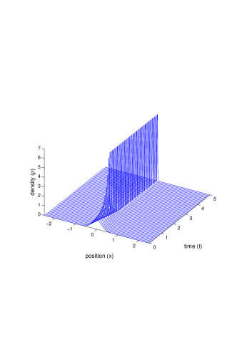
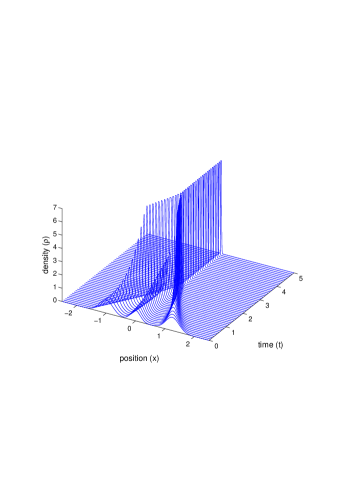
Figure 1: Dynamics of the density $\rho$ with two different intial data in the case $W=-\frac{1}{2}|x|$

In this case $W^{\prime\prime}=-\delta_{0}$. Then, setting $S=W*\rho$, we have that $-\partial_{xx}S=\rho$ and $-\partial_{x}S$ is an antiderivative of $\rho$. Then, integrating the aggregation equation, we can rewrite it as

$$\partial_{t}\partial_{x}S+\frac{1}{2}\partial_{x}\big{(}\partial_{x}S\big{)}^{2}=0.$$

We recognize the Burgers equation for $\partial_{x}S$. Moreover, in this particular case where $\nu_{i}^{n}=0$, we can deduce from (2.4)–(2.9) a scheme on $(\partial_{x}S_{i}^{n})_{i,n}$. First, (2.5) rewrites

$$J_{i+1/2}^{n}=-\frac{1}{\delta x}\big{(}A(\partial_{x}S_{i+1}^{n})-A(\partial_{x}S_{i}^{n})\big{)}.$$

Moreover, denoting $\rho_{i+1/2}^{n}=\frac{1}{2}(\rho_{i}^{n}+\rho_{i+1}^{n})$, we deduce from (2.9) and (2.7)

$$\rho_{i+1/2}^{n}=-\frac{1}{\delta x}\big{(}\partial_{x}S_{i+1}^{n}-\partial_{x}S_{i}^{n}\big{)}.$$

We deduce

$$\sum_{k=0}^{i}\rho_{k+1/2}^{n}=-\frac{1}{\delta x}\big{(}\partial_{x}S_{i+1}^{n}-\partial_{x}S_{0}^{n}\big{)}.$$

Equation (2.4) implies straightforwardly

$$\rho_{i+1/2}^{n+1}=\rho_{i+1/2}^{n}(1-\lambda c)+\frac{\lambda}{2}c(\rho_{i-1/2}^{n}+\rho_{i+3/2}^{n})+\frac{\lambda}{4}(J_{i-1/2}^{n}-J_{i+3/2}^{n}).$$

Summing this latter equation and using the boundary conditions $\partial_{x}S_{0}^{n}=0$, we deduce

$$\partial_{x}S_{i}^{n+1}=\partial_{x}S_{i}^{n}(1-\lambda c)+\frac{\lambda}{2}c(\partial_{x}S_{i-1}^{n}+\partial_{x}S_{i+1}^{n})-\frac{\lambda}{4}\big{(}A(\partial_{x}S_{i+1}^{n})-A(\partial_{x}S_{i-1}^{n})\big{)}.$$

In the case at hand where $a=id$, we have $A(x)=x^{2}/2$, we recognize the well-known Lax-Friedrichs discretization for the Burgers equation. Here we have $c=M$ where $M$ is the total mass of the system. Then the numerical results of Figure 1 was expected; we recover the convergence in finite time in a single Dirac mass as established for instance in [13, Section 4].

4.2 A kinetic model for chemotaxis

Let us consider the so-called Othmer-Dunbar-Alt model, describing the motion of cells by chemotaxis, in one dimension. This model has been used since the 80’s when it has been observed that the motion of bacteria is due to the alternance of straigth swim in a given direction, called run phase, with cells reorientation to choose a new direction, called tumble phase. This system governs the dynamics of the distribution function $f_{\varepsilon}$. In the hyperbolic scaling, it writes:

$$\partial_{t}f_{\varepsilon}+v\partial_{x}f_{\varepsilon}=\frac{1}{\varepsilon}\int_{V}\big{(}T[v^{\prime}\to v]f_{\varepsilon}(v^{\prime})-T[v\to v^{\prime}]f_{\varepsilon}(v)\big{)}\,dv^{\prime}.$$

In this equation $T[v^{\prime}\to v]$ is the turning rate, corresponding to the probability of cells to change their velocities from $v^{\prime}$ to $v$ during a tumble phase. In this work, we consider the model proposed by Dolak and Schmeiser [16] where

$$T[v^{\prime}\to v]=\phi(v^{\prime}\partial_{x}S_{\varepsilon}).$$

The function $\phi$ is given and assumed to be in $C^{1}(\mathbb{R})$. In this equation, the quantity $S_{\varepsilon}$ corresponds to the chemoattractant concentration which solves the elliptic equation

$$-\partial_{xx}S_{\varepsilon}+S_{\varepsilon}=\rho_{\varepsilon},$$ (4.1)

where $\rho_{\varepsilon}=\int_{V}f_{\varepsilon}(v)\,dv$ is the density of cells. This latter equation can be rewritten $S_{\varepsilon}=W*\rho_{\varepsilon}$ for $W=\frac{1}{2}e^{-|x|}$; therefore we have $W=w$ in (1.2).

The velocity $v$ is assumed to have a constant modulus, therefore the set of velocities in one dimension is given by $V=\{-v,v\}$. Then the kinetic equation rewrites in one dimension:

$$\partial_{t}f_{\varepsilon}+v\partial_{x}f_{\varepsilon}=\frac{1}{\varepsilon}(\phi(-v\partial_{x}S_{\varepsilon})f_{\varepsilon}(-v)-\phi(v\partial_{x}S_{\varepsilon})f_{\varepsilon}(v)).$$ (4.2)

Then the density of cells is defined by $\rho_{\varepsilon}:=f_{\varepsilon}(v)+f_{\varepsilon}(-v)$. Up to a rescaling, we assume that the turning rate satisfies

$$\phi(x)=\frac{1}{2}+\phi_{1}(x),\mbox{ with }\phi_{1}(-x)=-\phi_{1}(x)$$ (4.3)

so that $\phi(x)+\phi(-x)=1$, for all $x\in\mathbb{R}$. Then, we can rewrite (4.2) as

$$\partial_{t}f_{\varepsilon}+v\partial_{x}f_{\varepsilon}=\frac{1}{\varepsilon}(\phi(-v\partial_{x}S_{\varepsilon})\rho_{\varepsilon}-f_{\varepsilon}(v)).$$

We recognize the form (3.1) for the kinetic equation with $E(v,x)=\phi(-vx)$. Then the limiting model when $\varepsilon\to 0$ is given by (see Theorem 3.1)

$$\partial_{t}\rho+\partial_{x}J=0,\qquad J=-\partial_{x}A(\partial_{x}S)+a(\partial_{x}S)S,\qquad a(x)=-v\phi_{1}(vx).$$ (4.4)

This equation have been studied in [23].

Remark 4.1

As in the first example of this Section, we can recover an equation for the potential $S=W*\rho$, which turns out here to be nonlocal. Indeed, taking the convolution with $W=\frac{1}{2}e^{-|x|}$ of (4.4), we obtain

$$\partial_{t}S+A(\partial_{x}S)-W*A(\partial_{x}S)+\partial_{x}W*(a(\partial_{x}S)S)=0.$$

Then by recombining (4.1) and (4.4), this latter equation can rewrite

$$\partial_{t}S-\partial_{txx}S+\partial_{x}\big{[}-\partial_{x}A(\partial_{x}S)+a(\partial_{x}S)S\big{]}=0.$$

It bears some resemblance with the well-known Camassa-Holm equation [12], and exhibits the same peakon-like solutions. However the underlying dynamics is completely different and in the present case peakons collapse. Notice also that there are no anti-peakons because of the positivity of $\rho$.

4.2.1 Attractive case

The computational domain is assumed to be $[-2.5,2.5]$ and the velocity $v$ is normalized to 1. We consider the function $a(x)=-\phi_{1}(x)=2/\pi\mbox{ Arctan}(10x)$, which clearly satisfies (1.3).

We first consider the macroscopic model (4.4) and discretize the system thanks to (2.4)–(2.9), with $\nu_{i}^{n}$ replaced by $S_{i}^{n}$ in (2.9). Figure 2 displays the numerical results for the following initial data: $\rho^{ini}(x)=e^{-10(x-0.7)^{2}}+e^{-10(x+0.7)^{2}}$ (left) and $\rho^{ini}(x)=e^{-10(x-1.25)^{2}}+0.8e^{-20x^{2}}+e^{-10(x+1)^{2}}$ (right). As expected, we have a fast blow up of regular solution and a finite-time collapse in a single Dirac mass.

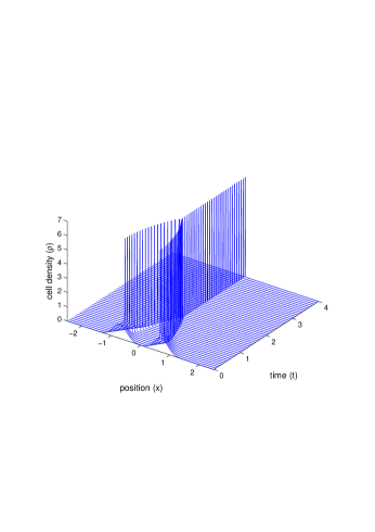
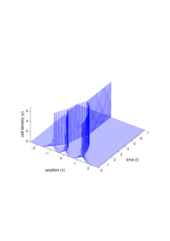
Figure 2: Macroscopic model (4.4): cell density $\rho$ for two regular bumps (left) and three regular bumps (right) initial data.

The behaviour of such Dirac solutions can be recovered by studying solutions in the form $\rho(t,x)=\sum_{i=1}^{n}m_{i}\delta(x-x_{i}(t))$. Then we have $S(t,x)=W*\rho(t,x)=\frac{1}{2}\sum_{i=1}^{n}m_{i}e^{-|x-x_{i}(t)|}$. After straightforward computations, we deduce from the expression in (4.4) that

$$J=-\sum_{i=1}^{n}[A(\partial_{x}S)]_{x_{i}}\delta(x-x_{i}(t)),$$

where the notation $[f]_{x_{i}}$ denotes the jump of the function $f$ at the point $x_{i}$. In particular, we have that $\rho$ satisfies system (4.4) provided,

$$m_{i}x^{\prime}_{i}(t)=-[A(\partial_{x}S)]_{x_{i}}.$$

Moreover, the function $a$ being increasing and odd, the function $A$ is strictly convex and can be chosen even. Then, equilibrium states satisfy

$$-[A(\partial_{x}S)]_{x_{i}}=A\Big{(}\frac{1}{2}\big{(}m_{i}+\sum_{j\neq i}m_{j}e^{-|x_{j}-x_{i}|}\big{)}\Big{)}-A\Big{(}\frac{1}{2}\big{(}-m_{i}+\sum_{j\neq i}m_{j}e^{-|x_{j}-x_{i}|}\big{)}\Big{)}=0.$$

This equality is true only if $\sum_{j\neq i}m_{j}e^{-|x_{j}-x_{i}|}=0$, which implies $n=1$. Therefore stationary states are given by a single stationary Dirac mass. Convergence towards this equilibrium is proved in [23, 13].

Then we consider the kinetic framework and implement the scheme described in Section 3. In Figure 3 and 4 we display the dynamics of the cell density $\rho$ for the regular initial data with two bumps: $\rho^{ini}(x)=e^{-10(x-0.7)^{2}}+e^{-10(x+0.7)^{2}}$ and an initial distribution function given by $f^{ini}(x,v)=\frac{1}{2}\rho^{ini}(x)$. We plot in the left part of the figures the numerical results corresponding to the macroscopic model (4.4), whereas the right part corresponds to numerical solution of (4.2). For the macroscopic case (left), we notice that the blow up occurs fastly. After a small time, solution is composed of 2 peaks which can be considered as numerical Dirac masses. Then the Dirac masses move and collapse in finite time. In the kinetic case (right), the solution does not blow up, as it is expected. However, the behaviour is similar to the one for the macroscopic model: we observe the formation of two aggregates that are in interaction and attract themselves in a single aggregate in finite time.

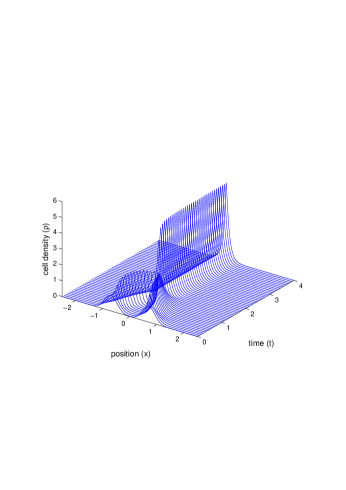
Figure 3: Dynamics of the cell density $\rho$ for an initial data given by a two regular bumps: comparison between the macroscopic model (left) and the kinetic model for $\varepsilon=0.1$ (right).

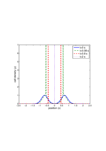
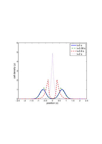
Figure 4: Dynamics of the cell density $\rho$ for an initial data given by a two regular bumps: comparison between the macroscopic model (left) and the kinetic model for $\varepsilon=0.1$ (right).

In Figure 5 we display the numerical results for different values of $\varepsilon$ and for a regular initial data given by the three bumps: $\rho^{ini}(x)=e^{-10(x-1.25)^{2}}+0.8e^{-20x^{2}}+e^{-10(x+1)^{2}}.$ As above, we notice the formation of 3 aggregates that merge into one single aggregate. When $\varepsilon\to 0$, we observe that the numerical solutions converges to the one computed in the macroscopic case, which is an illustration of the result of Theorem 3.2.

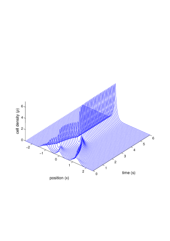
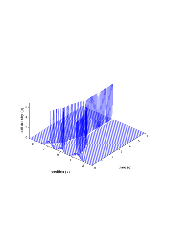
Figure 5: Dynamics of the cell density for an initial data given by a sum of 3 regular bumps: simulation of the kinetic model with $\varepsilon=0.1$ (left) and $\varepsilon=10^{-3}$ (right).

In the kinetic case, stationary state for (4.2) are given by

$$v\partial_{x}f_{\varepsilon}=\frac{1}{\varepsilon}(\phi(-v\partial_{x}S_{\varepsilon})\rho_{\varepsilon}-f_{\varepsilon}).$$

Summing the equation for $v$ and for $-v$, we deduce easily that we have that $f_{\varepsilon}(v)=f_{\varepsilon}(-v)$. Then, using the expression of $\phi$ in (4.3), the kinetic equation rewrites, for $v>0$,

$$v\partial_{x}f_{\varepsilon}=-\frac{1}{\varepsilon}\phi_{1}(v\partial_{x}S_{\varepsilon})f_{\varepsilon}.$$

Formally, if we consider that the function $\phi_{1}$ is an approximation of the function $-sign$. Then, the latter equation is a linear ODE which can be solved easily and implies that $f$ is given by the sum of exponential function with the tail $\pm\frac{1}{\varepsilon v}$. This behaviour corresponds to what is observed in Figure 4 right.

Finally, we emphasize the importance of the choice of the discretized macroscopic velocity. For instance, in the aggregation equation (1.1), if instead of defining the discretization (2.8) we take $a_{i+1/2}^{n}=a((S_{i+1}^{n}-S_{i}^{n})/\delta x)$, we obtain Figure 6, to be compared with Figure 3.

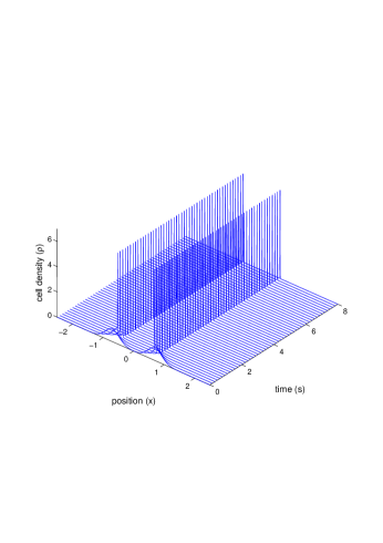
Figure 6: Wrong velocity discretization for (1.1)

Concerning the kinetic model, we display in Figure 7 the results obtained when the discretization of $E_{ij}^{n}$ in (3.17) is replaced by $E_{ij}^{n}=E(v_{j},\partial_{x}S_{i}^{n})$, with $\partial_{x}S_{i}^{n}=(S_{i+1}^{n}-S_{i-1}^{n})/2\delta x$. We notice in Figure 7(left) that for $\varepsilon=10^{-3}$ the behaviour of the density remains comparable with the macroscopic model (see Figure 2). When $\varepsilon$ goes to zero, namely here $\varepsilon=10^{-5}$, we observe the same kind of result as for the macroscopic case, compare Figures 7(right) and 6.

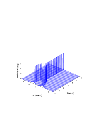
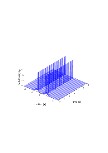
Figure 7: Wrong velocity discretization for kinetic model: $\varepsilon=10^{-3}$ (left) – $\varepsilon=10^{-5}$ (right)

4.2.2 Repulsive case

Finally, we conclude this paper with some numerical results without any proof in the repulsive case i.e. when the function $a$ is non-increasing. Then assumption (1.3) is not satisfied and the velocity $x\mapsto a(\partial_{x}S)$ does not satisfy the one-sided Lipschitz estimate (2.1). However, it can be proved (using the arguments in e.g. [34]) that if $\rho^{ini}\in L^{1}\cap W^{1,\infty}(\mathbb{R})$, we have global in time existence of weak solutions in $L^{1}\cap W^{1,\infty}(\mathbb{R})$. Using the dynamics of Dirac masses to design a particle scheme is therefore not straghtforward in this case. In this respect, we refer to [7], where gradient flow solutions are proved to be equivalent to entropy solutions of the Burgers equation, with a particular focus on the repulsive case. A particle discretization is also proposed. It is then interesting to implement our numerical discretization (2.4)–(2.5) for the macroscopic model (4.4) in the repulsive case.

Figure 8 displays the numerical results for $a(x)=-2/\pi\mbox{ Arctan}(10x)$ (left) and for $a(x)=-2/\pi\mbox{ Arctan}(50x)$ (right) with the initial data $\rho^{ini}(x)=e^{-10x^{2}}$. Figure 9 displays the dynamic of the cells density for $a(x)=-2/\pi\mbox{ Atan}(10x)$ and for the initial data $\rho^{ini}(x)=e^{-10(x-0.7)^{2}}+e^{-10(x+0.7)^{2}}$.

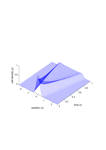
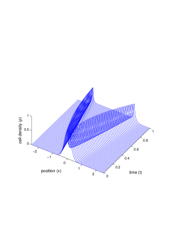
Figure 8: Dynamics of the cell density in the repulsive case, i.e. for a non-increasing function $a(x)=-2/\pi\mbox{ Atan}(kx)$. Left: $k=10$; Right: $k=50$.

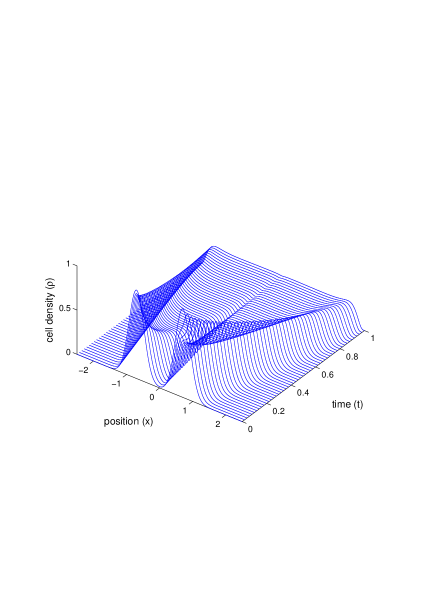
Figure 9: Dynamics of the cell density for an initial data given by a sum of 2 regular bumps in the repulsive case for $a(x)=-2/\pi\mbox{ Atan}(10x)$.

References

• [1] L. Ambrosio, N. Fusco, D. Pallara, Functions of Bounded Variation and Free Discontinuity Problems, Oxford University Press, 2000
• [2] L. Ambrosio, N. Gigli, G. Savaré, Gradient flows in metric space of probability measures, Lectures in Mathematics, Birkäuser, 2005
• [3] D. Benedetto, E. Caglioti, M. Pulvirenti, A kinetic equation for granular media, RAIRO Model. Math. Anal. Numer., 31 (1997), 615–641
• [4] A.L. Bertozzi, J. Brandman, Finite-time blow-up of $L^{\infty}$-weak solutions of an aggregation equation, Comm. Math. Sci., 8 (2010), no 1, 45–65
• [5] A.L. Bertozzi, J.A. Carrillo, T. Laurent, Blow-up in multidimensional aggregation equation with mildly singular interaction kernels, Nonlinearity 22 (2009), 683–710
• [6] A.L. Bertozzi, T. Laurent, Finite-time blow-up of solutions of an aggregation equation in $\mathbb{R}^{n}$, Comm. Math. Phys., 274 (2007), 717–735
• [7] G. Bonaschi, J.A. Carrillo, M. Di Francesco, M. Peletier, Equivalence of gradient flows and entropy solutions for singular nonlocal interaction equations in 1D, preprint arXiv:1310.4110 http://arxiv.org/abs/1310.4110
• [8] F. Bouchut, F. James, One-dimensional transport equations with discontinuous coefficients, Nonlinear Analysis TMA 32 (1998), no 7, 891–933
• [9] F. Bouchut, F. James, Duality solutions for pressureless gases, monotone scalar conservation laws, and uniqueness, Comm. Partial Differential Eq., 24 (1999), 2173–2189
• [10] N. Bournaveas, V. Calvez, S. Gutièrrez, B. Perthame, Global existence for a kinetic model of chemotaxis via dispersion and Strichartz estimates, Comm. Partial Differential Eq., 33 (2008), 79–95.
• [11] M. Burger, V. Capasso, D. Morale, On an aggregation model with long and short range interactions, Nonlinear Anal. Real World Appl. (2007) 8, 939–958
• [12] R. Camassa, D. Holm, An integrable shallow water equation with peaked solitons, Phys. Rev. Lett., 71 (1993), 1661–1664
• [13] J. A. Carrillo, M. DiFrancesco, A. Figalli, T. Laurent, D. Slepčev, Global-in-time weak measure solutions and finite-time aggregation for nonlocal interaction equations, Duke Math. J. 156 (2011), 229–271
• [14] R.M. Colombo, M. Garavello, M. Lécureux-Mercier, A class of nonlocal models for pedestrian traffic, Math. Models Methods Appl. Sci., (2012) 22(4):1150023, 34.
• [15] G. Crippa, M. Lécureux-Mercier, Existence and uniqueness of measure solutions for a system of continuity equations with non-local flow, Nonlinear Differential Equations Appl. (NoDEA), 20 (2013), no 3, 523–537
• [16] Y. Dolak, C. Schmeiser, Kinetic models for chemotaxis: Hydrodynamic limits and spatio-temporal mechanisms, J. Math. Biol. 51, 595–615 (2005).
• [17] F. Filbet, Ph. Laurençot, B. Perthame, Derivation of hyperbolic models for chemosensitive movement, J. Math. Biol., 50 (2005), 189–207.
• [18] F. Filbet, S. Jin, A class of asymptotic-preserving schemes for kinetic equations and related problems with stiff sources, J. Comput. Phys., 229 (2010), 7625–7648
• [19] L. Gosse, Asymptotic-preserving and well-balanced schemes for the 1D Cattaneo model of chemotaxis movement in both hyperbolic and diffusive regimes, J. Math. Anal. Appl. 388 (2012), no 2, 964–983
• [20] L. Gosse, A well-balanced scheme for kinetic models of chemotaxis derived from one-dimensional local forward-backward problems, Mathematical Biosciences, to appear.
• [21] L. Gosse, G. Toscani, Space localization and well-balanced schemes for discrete kinetic models in diffusive regimes, SIAM J. Numer. Anal. 41 (2003), no 2, 641–658
• [22] F. James, N. Vauchelet, On the hydrodynamical limit for a one dimensional kinetic model of cell aggregation by chemotaxis, Riv. Mat. Univ. Parma., 3 (2012), 91–113
• [23] F. James, N. Vauchelet, Chemotaxis: from kinetic equations to aggregate dynamics, Nonlinear Diff. Eq. Appl. NoDEA, 20 (2013), Issue 1, 101–127
• [24] F. James, N. Vauchelet, Numerical simulation of a hyperbolic model for chemotaxis after blow-up, preprint http://hal.archives-ouvertes.fr/hal-00772653/fr/, to appear in Proceedings of 14 Conference on Hyperbolic Problems, Padova, Italy (2012)
• [25] F. James, N. Vauchelet, Equivalence between duality and gradient flow solutions for one-dimensional aggregation equations, preprint http://hal.archives-ouvertes.fr/hal-00803709/fr/
• [26] S. Jin, Asymptotic preserving (AP) schemes for multiscale kinetic and hyperbolic equations: a review, Riv. Mat. Univ. Parma, 3 (2012), 177–216
• [27] S. Jin, Efficient asymptotic-preserving (AP) schemes for some multiscale kinetic equations, SIAM J. Sci. Comput., 21 (1999), no 2, 441–454
• [28] S. Jin, L. Pareschi, Discretization of the multiscale semiconductor Boltzmann equation by diffusive relaxation schemes, J. Comput. Phys. 161 (2000), no 1, 312–330
• [29] S. Jin, L. Pareschi, G. Toscani, Uniformly accurate diffusive relaxation schemes for multiscale transport equations, SIAM J. Num. Anal. 38 (2001), no 3, 913–936
• [30] M. Lemou, L. Mieussens, A new asymptotic preserving scheme based on micro-macro formulation for linear kinetic equations in the diffusion limit, SIAM J. Sci. Comput., 31 (2008), no 1, 334–368
• [31] A.J. Leverentz, C.M. Topaz, A.J. Bernoff, Asymptotic dynamics of attractive-repulsive swarms, SIAM J. Appl. Dyn. Systems, 8 No 3, 880–908
• [32] H. Li, G. Toscani, Long time asymptotics of kinetic models of granular flows, Arch. Rat. Mech. Anal., 172 (2004), 407–428
• [33] D. Morale, V. Capasso, K. Oelschläger, An interacting particle system modelling aggregation behavior: from individuals to populations, J. Math. Biol., 50 (2005), 49–66
• [34] J. Nieto, F. Poupaud, J. Soler, High field limit for Vlasov-Poisson-Fokker-Planck equations, Arch. Rational Mech. Anal. 158 (2001), 29–59
• [35] A. Okubo, S. Levin, Diffusion and Ecological Problems: Modern Perspectives, Springer, Berlin, 2002
• [36] N. Vauchelet, Numerical simulation of a kinetic model for chemotaxis, Kinetic and Related Models 3 (2010), no 3, 501–528
• [37] A.I. Vol’pert, The spaces BV and quasilinear equations, Math. USSR Sb., 2 (1967), 225–267