Microscopic Calibration and Validation of Car-Following Models – A Systematic Approach

Abstract

Calibration and validation techniques are crucial in assessing the descriptive and predictive power of car-following models and their suitability for analyzing traffic flow. Using real and generated floating-car and trajectory data, we systematically investigate following aspects: Data requirements and preparation, conceptional approach including local maximum-likelihood and global LSE calibration with several objective functions, influence of the data sampling rate and measuring errors, the effect of data smoothing on the calibration result, and model performance in terms of fitting quality, robustness, parameter orthogonality, completeness and plausible parameter values.

1 Introduction

Microscopic traffic flow models describe the driving behavior, local traffic rules, and possible restrictions of the vehicle. All these aspects vary with the driver but also with the country and with time. For example, drivers in the United States and in Germany have different driving styles, drive different types of vehicles and are subject to different traffic regulations. For drivers in China, the differences are even more pronounced. Furthermore, traffic flow on a given road is generally more effective during the morning rush hours than in the evening rush hours or at night since drivers are generally more alert and drive more effectively in the morning than at other times. Consequently, not even the best model reproducing all traffic flow situations in question can be applied to a specific task with the default parameter set. Instead, to maximize the model’s descriptive power, its parameters need to be estimated based on representative traffic data.

Nevertheless, only few systematic investigations have been undertaken on this topic. While collective macroscopic aspects of traffic flow such as travel times or traffic waves can be calibrated and validated on macroscopic data [1, 2], it is more natural to calibrate car-following models on microscopic data sets. These include single-vehicle data of stationary detectors, extended floating-car data (xFCD) [3, 4, 5, 6, 7], and trajectory data [8, 9, 10]. Trajectory data such as these of the NGSIM project [11, 12] contain the dynamics of the positions (and lanes) of all vehicles in a given spatiotemporal region. In contrast, xFC data (which typically are generated by instrumented vehicles) include, for only one or a few vehicles, time series of the position, the speed, and the gap to the respective leading vehicle.

Regarding calibration and validation, many questions are not yet settled: What is the minimum quantitative data requirement for a given calibration task in terms of the minimal set of observed quantities, minimum number of vehicles, minimum length of time interval, or minimum temporal resolution? Is it possible to formulate qualitative data requirements by defining a minimal set of traffic states which must be contained in the data [13]? To which degree does data noise or the sampling rate influence the calibration result [10]? Is it possible to distinguish noise from intra-driver and inter-driver variations [14, 15, 16]? To which degree does the result differ when calibrating a given model on given data with different methods such as least squared errors (LSE), maximum-likelihood, or Kalman filtering [17, 18, 1]? How does the result depend on the objective function [5, 6]? Why is there so little difference when comparing LSE calibration results of the “best” with that of the “worst” models [3]? Are there more suitable criteria than the fitting quality, e.g., sensitivity with respect to parameter changes [19] or robustness?

In this contribution, we systematically investigate these aspects using both real and generated data. While, ultimately, the quality of models and calibration techniques is to be assessed by real data, generated data allow for separating the influencing factors in a systematic and controlled way.

In principle, this program can be performed with any car-following model specifying the acceleration, either directly or indirectly in terms of speed differences [7]. For the sake of demonstration, we will use mainly the intelligent-driver model (IDM) [20, 7]. It is suited for this kind of investigations since the meaning of its five parameters is intuitive and each parameter relates to a certain driving regime: The desired speed $v_{0}$ is relevant for cruising in free-traffic conditions, the desired time gap $T$ pertains to steady-state car-following, the minimum gap $s_{0}$ to creeping and standing traffic, and the maximum acceleration $a$ and desired deceleration $b$ relate to non-steady-state traffic flow. For cross comparison, we will also use the optimal-velocity model (OVM)[21] and the full-velocity difference model [22]. However, we will use these models together with modified steady-state speed-gap relations also containing the parameters $s_{0}$ and $T$ instead of the original ones with non-intuitive parameters.

After discussing methodic data, calibration, and simulation issues in the next two sections, we investigate the influence of the data sampling rate, noise, serial correlations, and smoothing in Sec. 4 before discussing the more model-related issues data and model completeness as well as parameter orthogonality in Sec. 5. We conclude this contribution by a discussion and hints for further research in Sec. 6.

2 Data Issues

Since car-following models are supposed not only to describe the microscopic dynamics of individual drivers but also macroscopic aspects of traffic flow (traffic waves, traffic jam propagation, or travel times) emerging from the dynamics, such models can, in principle, be calibrated and validated by both microscopic and macroscopic data. Nevertheless, it is more natural to use microscopic data of individual drivers. Since this allows to separate the effects of inter-driver variations (different drivers have different driving styles) from intra-driver variations (even one and the same driver may change his or her driving behavior over time) [14, 15, 16], this gives more control when investigating the models.

We consider two categories of individual-driver data: Extended floating-car data (xFCD) come in the form of time series for the (arc-length) positions $x_{i}=x^{\rm data}(t_{i})$, speeds $v_{i}=v^{\rm data}(t_{i})$, and (bumper-to-bumper) gaps $s_{i}=s_{i}^{\rm data}(t_{i})$ at times $t_{i}=t_{0}+i\,\Delta t$. Here, $i$ denotes the time step and $\Delta t$ is the sampling interval (inverse of the sampling rate). Since $\frac{{\rm d}x}{{\rm d}t}=v$, positions and speed are not independent and only one of them can be considered as the primary quantity and the other as derived quantity. In any case, the gap is measured independently and directly by a range sensor. In this contribution, we use three sets of xFCD which are captured by an instrumented car (sampling rate 10 Hz) driven through a German inner-city street by three different drivers (cf. Fig. 1).

Fig. 1: Sets 1 and 3 of extended floating-car data of a car driving in a German city during rush-hour conditions. In the set labelled 3, the leader leaves the lane at $t\approx 144\,\mathrm{s}$ resulting in a discontinuity in the time series for the gap.

Since this vehicle was not equipped with high-precision (differential) GPS, we consider the speed and gap measurements as primary data, i.e., we derive the positions (or rather, displacements) of the follower and the leader from the speed of the follower and the gap (between leader and follower) rather than vice versa.

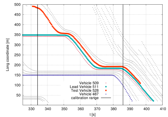
Fig. 2: Example of trajectories from the NGSIM project. Shown is a spatiotemporal region of the Lankershim set (every 5th data point is displayed) for direction 4 and lane 2. Vehicles 528 and 509 represent “complete” data containing all traffic situations while Vehicle 487 includes minimum-gap and acceleration information, only. Stopping lines of traffic lights are located at approximatively 145 m and 340 m. Vehicle 528 with its leader 511 will be investigated in the calibration example later on. All other trajectories in this region are dotted.

Trajectory data provide the locations (and lanes) of all vehicles in a given spatiotemporal region, so it is straightforward to extract the (arc-length) positions $x_{i}$ and $x_{li}$ of the considered vehicle and of its leader, respectively. Several freeway and arterial data sets are made available by the NGSIM project [23]. It turned out that the data cannot be used directly since they contain all sorts of inconsistencies and errors [11, 12] which significantly influences the calibration results, particularly for the less robust models. Figure 2 shows an extract of these data where no obvious discrepancies are observed.

The NGSIM data, and to a lesser extent the inner-city xFCD data, contain negative speeds, negative gaps, unreasonable values for accelerations, unreasonable frequency of sign changes for accelerations, and sudden “jumps” of vehicles forwards, backwards, or to the side. Furthermore, both the xFCD and NGSIM data contain positions, speeds, and accelerations, i.e., partially redundant information, and it is not always documented how the dependent quantities are determined. Moreover, they generally violate basic kinematic constraints, particularly, that of internal consistency,

$$\frac{{\rm d}x}{{\rm d}t}=v(t),\quad\frac{{\rm d}v}{{\rm d}t}=\dot{v}(t),$$ (1)

and that of platoon consistency [24]

$$s(0)=x_{l}(0)-x(0)-l_{l},\quad\frac{{\rm d}s}{{\rm d}t}=v_{l}(t)-v(t).$$ (2)

Here, $x(t)$ and $x_{l}(t)$ are the arc-length positions of the front bumper of the considered and leading vehicles, respectively, $v(t)$ and $v_{l}(t)$ the corresponding speeds, $s(t)$ denotes the bumper-to-bumper gap in between, and $l_{l}$ denotes the length of the leading vehicle. We focus on calibrating car-following models of the generic form

$$\dot{v}(t)\equiv\frac{{\rm d}v}{{\rm d}t}=a_{\rm mic}(s,v,v_{l},\dot{v}_{l})$$ (3)

returning as endogeneous variable (dependent or output variable) the acceleration $\dot{v}(t)$ as a function of the gap and the speeds of the considered and leading vehicles. The function $a_{\rm mic}(.)$ specifies the car-following model in question. Some models such as the ACC model [25] also include the leading acceleration $\dot{v}_{l}$. If reaction times are modelled explicitely, some or all of the above exogeneous variables (also denoted as independent or input model variables) are taken at a delayed time. Discrete-time models such as Gipps’ model can be cast into this form by formulating the acceleration in terms of finite speed differences which these models provide, $\dot{v}(t)=[v(t+\Delta t_{\rm sim})-v(t)]/\Delta t_{\rm sim}$ where $\Delta t_{\rm sim}$ denotes the model update time interval which is not necessarily identical to the interval $\Delta t$ between two data points. In order to obtain consistent training data sets for calibration, i.e., time series of the exogeneous model variables $s(t)$, $v(t)$, and $v_{l}(t)$ as well as the endogeneous acceleration, we ignore all redundant (and inconsistent) information provided by the data sets. Instead, we calculate it from the directly measured data using the consistency criteria.

As already mentioned, the directly measured xFCD quantities are the gaps $s_{i}$ (measured by the range sensor) and the speed values $v_{i}$. After setting negative gap and speed values equal to zero, we calculate the remaining variables using Conditions (1) and (2) by the following finite differences:

$$v_{li}=v_{i}+\frac{s_{i+1}-s_{i-1}}{2\Delta t},\quad\dot{v}_{i}=\frac{v_{i+1}-v_{i-1}}{2\Delta t},\quad\dot{v}_{li}=\dot{v}_{i}+\frac{s_{i+1}-2s_{i}+s_{i-1}}{(\Delta t)^{2}}.$$ (4)

Discontinuities of the gap time series of xFCD are not necessarily artifacts but may be the result of active lane changes (the driver of the instrumented vehicle changes lanes), passive cut-out lane changes (the leader changes to another lane as in Set 3 of Fig. 1 at $t\approx 144\,\mathrm{s}$), or passive cut-in changes (a new vehicle changes into the gap before the instrumented vehicle). We notice that positions and vehicle lengths are not contained in the set of exogeneous variables of the considered class of car-following models. These quantities are neither known for the investigated xFCD data nor needed for microscopic calibration.

The primary quantities of the NGSIM data are the positions, particularly the positions $x_{i}$ and $x_{li}$ of a pair of vehicles following each other at times $t_{i}=t_{0}+i\Delta t$. We calculate the gap by

$$s_{i}=x_{li}-x_{i}-l_{i}.$$ (5)

Notice that we require that the data contain the vehicle length of the leader and a definition whether $x$ denotes the position of the front bumper (for which the above relation is valid), or another well-specified position. Afterwards, we check for negative gaps or backwards moving vehicles and calculate the dependent quantities $v_{i}$, $v_{li}$, and $\dot{v}_{i}$ by the appropriate symmetric finite differences,

$$v_{i}=\frac{x_{i+1}-x_{i-1}}{2\Delta t},\quad v_{li}=\frac{x_{l,i+1}-x_{l,i-1}}{2\Delta t},\quad\dot{v}_{i}=\frac{x_{i+1}-2x_{i}+x_{i-1}}{(\Delta t)^{2}},$$ (6)

thereby ensuring internal and platoon consistency.

When testing the effects of different sampling rates or data smoothing (Sec. 4), we resample the primary data and/or apply kernel-based moving averages (with Gaussian kernels of a certain width $w$) on them before calculating the remaining quantities with (4) or (6), respctively. In this way, we ensure that the smoothed or re-sampled data are consistent as well.

Finally, in order to have more control over the traffic situations in Sec. 4, we also use generated data of vehicle platoons produced by microscopic simulations with a specified car-following model and a prescribed speed profile for the leading vehicle (cf. Fig. 8 below). By virtue of the simulation, these data are automatically consistent. Calibrating a model to data produced by the same model is the only methodologocal means to undertake investigations requiring knowledge of the true parameters, e.g., when investigating the bias introduced by smoothing or noise (Section 4.2).

3 Approaches to Calibration

We investigate two approaches: In the local approach, the endogenous model variable (speed change or acceleration) is compared against the data, separately for each data point, by maximum-likelihood techniques [26]. In the global approach, we compare a complete data trajectory with a simulated trajectory and define an objective function in terms of a sum of squared errors (SSE) of gaps or speeds. Since we focus on model properties rather than on real-time traffic state estimation, we will not investigate calibration by extended Kalman filters where the parameters and the traffic state are estimated simultaneously by maximum-likelihood techniques [17, 18, 1].

While the local approach is purely model based, the global approach can be considered as simulation based [27]: Each calculation of the objective function involves a complete simulation run.

3.1 Local Maximum-Likelihood Calibration

This approach assumes explicit noise of a given distribution, either in the model (stochastic car-follownig models), or in the data, or in both. For each time instance $t_{i}$, the data contain the vector $\vec{x}_{i}$ of all exogeneous variables needed for the model and the vector $\vec{y}_{i}$ of all endogeneous variables. This enables us to define the likelihood function as the joint probability that the model predicts all data points given a certain parameter vector $\vec{\beta}$:

$$L(\vec{\beta})={\mbox{ prob}}\left(\hat{\vec{y}}_{1}(\vec{\beta})=\vec{y}_{1},\ \ldots,\ \hat{\vec{y}}_{n}(\vec{\beta})=\vec{y}_{n}\right).$$ (7)

If we assume zero-mean Gaussian multivariate noise with fixed but unknown covariance matrix $\Sigma$ which is iid with respect to different time steps (no serial correlation), the log-likelihood $\tilde{L}(\vec{\beta})=\ln L(\vec{\beta})$ becomes [26]

$$\tilde{L}(\vec{\beta},\Sigma)={\mbox{ const.}}-\frac{n}{2}\ln({\mbox{ det}}\,\Sigma)-\frac{1}{2}\sum\limits_{i=1}^{n}\vec{e}_{i}^{{\mbox{ T}}}(\vec{\beta})\,\Sigma^{-1}\vec{e}_{i}(\vec{\beta})$$ (8)

where

$$\vec{e}_{i}(\vec{\beta})=\hat{\vec{y}}_{i}(\vec{\beta})-\vec{y}_{i}$$ (9)

denotes the vector of deviations at time $t_{i}$. Estimating the covariance matrix by

$$\hat{\Sigma}(\vec{\beta})=\frac{1}{n}\sum\limits_{i=1}^{n}\vec{e}_{i}(\vec{\beta})\,\vec{e}_{i}^{{\mbox{ T}}}(\vec{\beta})$$ (10)

allows us to formulate the log-likelihood

$$L^{*}(\vec{\beta})=\tilde{L}\left(\vec{\beta},\hat{\Sigma}(\vec{\beta})\right)$$ (11)

as a function of the parameter vector $\vec{\beta}$ alone. This is the basis for parameter estimation:

$$\hat{\vec{\beta}}={\mbox{ arg}}\ \max L^{*}(\vec{\beta}).$$ (12)

When calibrating models of the form (3) on the motion of single vehicles, there is only one endogeneous variable which is given by the acceleration, i.e., $\hat{\vec{y}}_{i}=a_{i}^{\rm mic}$ and $\vec{y}_{i}=\dot{v}_{i}$ for the predictions and observations, respectively. Augmenting models of the form (3) by iid acceleration noise,

$$\frac{{\rm d}v}{{\rm d}t}=a_{\rm mic}(s,v,v_{l};\vec{\beta})+\epsilon,\quad\epsilon\sim iid\;N(0,\sigma^{2}),$$ (13)

or assuming that the observed accelerations have this sort of noise, we can derive from (12) the explicit calibration condition

$$\hat{\vec{\beta}}={\mbox{ arg}}\ \min S_{\rm ML}(\vec{\beta}),\quad S_{\rm ML}(\vec{\beta})=\sum\limits_{i=1}^{n}\left(\dot{v}_{i}-a_{i}^{\rm mic}(\vec{\beta})\right)^{2}\,,$$ (14)

where $a_{i}^{\rm mic}(\vec{\beta})=a_{\rm mic}(s_{i},v_{i},v_{li},\dot{v}_{li};\vec{\beta})$ and $S_{\rm ML}(\vec{\beta})$ is related (but not identical) to $-\ln L(\vec{\beta})$. Since the statistical properties are specified explicitely, the statistical properties of the parameter estimates are, in principle, known: Its covariance matrix is given in terms of the inverse Hessian of $-\ln L(\vec{\beta})$ which is provided by most nonlinear optimization packages. However, in contrast to the iid assumption in deriving this matrix, the deviations $e_{i}$ are serially correlated which can be seen by comparing the estimated and observed accelerations of Fig. 3. Consequently, the error estimates are not valid. As we will show in Sec. 4, even the estimates of the parameters themselves may be biased.

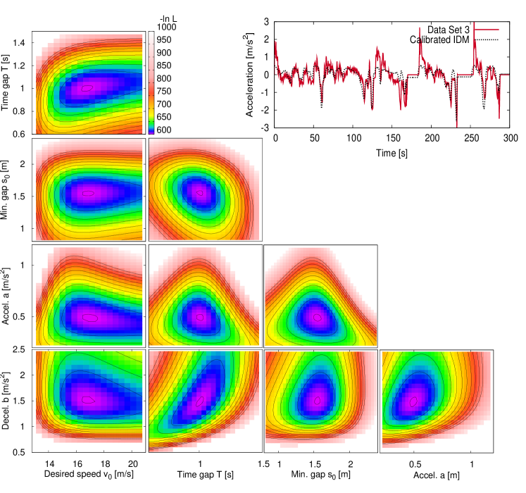
Fig. 3: Local maximum-likelihood calibration of the IDM to the xFCD Set 3. Shown are the model accelerations for the calibrated parameters shown in the left column of Table 1, and contour plots of the objective function (14) for two-dimensional sections of the five-dimensional parameter space around the estimation.

IDM parameter	local calibration	global calibration (16)	global calibration (17)
desired speed $v_{0}[\mathrm{m/s}]$	16.9	16.1	16.1
desired time gap $T[\mathrm{s}]$	1.02	1.27	1.20
minimum gap $s_{0}[\mathrm{m}]$	1.56	1.44	1.53
maximum acceleration $a[\mathrm{m/s^{2}}]$	0.51	1.46	1.39
comfortable deceleration $b[\mathrm{m/s^{2}}]$	1.47	0.63	0.65

Table 1: calibration of the IDM to the xFCD Set 3 with respect to three objective functions.

Figure 3 shows the result when calibrating the five parameters of the intelligent-driver model (IDM) [20] to the xFCD Set 3 (cf. Fig. 1). We observe that the “fitting landscape” of the objective function $S_{\rm ML}(\vec{\beta})$ is smooth and contains a unique global minimum. This allows us to apply the efficient Levenberg-Marquardt algorithm for solving the nonlinear multivariate minimization problem (14). We have used the open-source package levmar[28]. A calibration of a five-parameter model to the $\approx 3\,000$ xFC data points takes a few milliseconds. As result of the calibration, four of the five estimated IDM parameters (desired speed $v_{0}$, desired time gap $T$, minimum gap $s_{0}$, and comfortable deceleration $b$) assume plausible values while the value of the acceleration parameter $a$ is unrealistically low.

3.2 Global Least-Squared Errors Calibration

In the more commonly used global approach to trajectory calibration, we do not calibrate the model directly by independently comparing the endogeneous model variables with the observations, step by step. Rather, we use simulations of the model to obtain predicted trajectories which, then, are compared with the observed trajectories by formulating objective functions in terms of sums of squared errors (SSE) of appropriate variables $\vec{y}$,

$$S(\vec{\beta})=\sum\limits_{i=1}^{n}\left(\hat{\vec{y}}_{i}(\vec{\beta})-\vec{y}_{i}\right)^{2}.$$ (15)

Similarly to the local ML approach, minimizing this function reduces the calibration problem to a multi-variate nonlinear optimization problem. In fact, (15) includes the objective function (14) by setting $\vec{y}_{i}=\dot{v}_{i}$. However, it turns out that neither accelerations nor speeds are suited as basis for the SSE of the simulation-based global approach since a speed-based measure would be insensitive to parameters controlling the gaps (e.g., $s_{0}$ and $T$ for the IDM), and acceleration-based measures are additionally insensitive to the desired speed $v_{0}$. This agrees also with the findings of Punzo and Simonelli [29]. We therefore investigate absolute and relative measures of the gap differences by defining the objective functions

$$S_{s}^{\rm abs}(\vec{\beta}) = \sum\limits_{i=1}^{n}\left(\hat{s}_{i}(\vec{\beta})-s_{i}\right)^{2},$$ (16)

$$S_{s}^{\rm rel}(\vec{\beta}) = \sum\limits_{i=1}^{n}\left(\ln\hat{s}_{i}(\vec{\beta})-\ln s_{i}\right)^{2}=\sum\limits_{i=1}^{n}\left[\ln\left(\frac{\hat{s}_{i}(\vec{\beta})}{s_{i}}\right)\right]^{2}$$ (17)

When applying (16), the focus is on larger gaps corresponding to acceleration or free-flow regimes (for the IDM, this relates to the parameters $v_{0}$ and $a$) while (17) considers all regimes. In contrast to [5, 6], we use as measure of the relative deviation the logarithm $e_{i}=\ln(\hat{s}_{i}/s_{i})$ rather than the ratio $(\hat{s}_{i}-s_{i})/s_{i}$ . While both measures are equivalent to first order,

$$e_{i}=\ln\left(\frac{\hat{s}_{i}}{s_{i}}\right)=\frac{\hat{s}_{i}-s_{i}}{s_{i}}+{\cal O}\left(\frac{\hat{s}_{i}-s_{i}}{s_{i}}\right)^{2},$$ (18)

the objective function (17) is less sensitive to outliers and measuring errors.

In order to obtain the simulation-based estimates $\hat{s}_{i}$, we initialize the speed of the simulated vehicle and its initial gap to the leading vehicle by the data and let the vehicle follow the fixed observed speed profile $v_{l}(t)$ of its leader as obtained by (4):

$$\frac{{\rm d}\hat{v}}{{\rm d}t}=a_{\rm mic}(\hat{s},\hat{v},v_{l};\vec{\beta}),\quad\hat{s}(t_{0})=s(t_{0}),\ \hat{v}(t_{0})=v(t_{0}).$$ (19)

We treat discontinuities caused by active or passive lane changes (as in the xFCD Set 3 at $t\approx 144\,\mathrm{s}$) in the same way as a range sensor of an adaptive cruise control system detecting a new target would do, i.e., by introducing a data-driven discontinuity of the simulated gap:

$$\hat{s}(t^{+})=\hat{s}(t^{-})+s(t^{+})-s(t^{-})$$ (20)

where $t^{-}$ and $t^{+}$ denote the times immediately before and after the detection of the new target, respectively. To determine whether such a discontinuity has occurred, we compare the ballistic extrapolation

$$\hat{s}_{\rm ball}(t_{i}+\Delta t;\Delta a)=s_{i}+(v_{li}-v_{i})\Delta t+\frac{1}{2}\Delta a(\Delta t)^{2}$$ (21)

with the observation $s_{i+1}$. The event “a new target is detected” is triggered if $\hat{s}_{\rm ball}(t_{i}+\Delta t;\Delta a)=s_{i+1}$ is not true for any acceleration difference in the range $|\Delta a|<20\,\mathrm{m/s^{2}}$.

Instead of (20), we also tested a “hard reset” according to

$$\hat{s}(t^{+})=s(t^{+}),\quad\hat{v}(t^{+})=v(t^{+})$$ (22)

which turned out to produce little differences. The reset has the advantage that multiple trajectories can be calibrated simultaneously by concatenating the corresponding data and evaluating the objective function by running a single car-following simulation which is controlled by the resulting compound xFCD via (19) and (22).

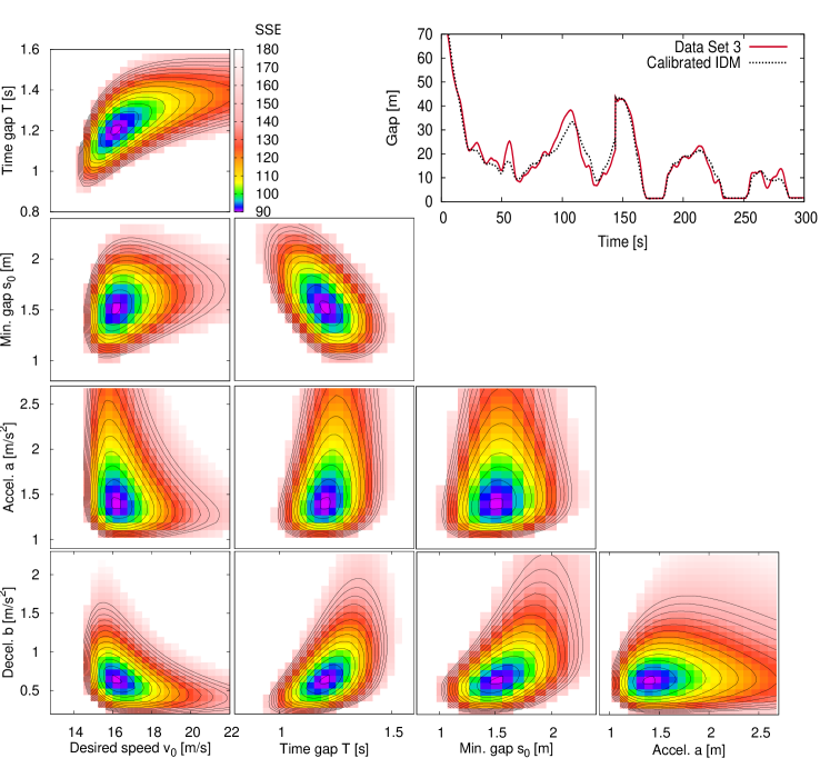
Fig. 4: Global calibration of the IDM to the xFCD Set 3 with respect to the logarithms of the gaps. Shown are the observed and simulated gaps for the calibrated parameters (Table 1, right column) and contour plots of the objective function (17) for two-dimensional sections of the five-dimensional parameter space around the estimation.

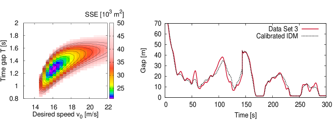
Fig. 5: Global calibration of the IDM to the xFCD Set 3 with respect to the gaps.

Fig. 6: Global calibration of Vehicle 528 of the NGSIM Lankershim data set (for the trajectories, see Fig. 2) with respect to the gap deviations in the time interval [334 s,386 s]. Shown is the fitting quality with respect to the gaps and speeds and two-dimensional subsets of the objective function around the calibrated parameters. Obviously, the objective function is smooth and unimodal.

Finally, we need to treat the case that the range of suitable or prescribed simulation update time intervals $\Delta t_{\rm sim}$ is incompatible with the sampling interval $\Delta t$. This applies to most of the time-discrete car-following models (e.g., Gipps’ model [30] or Newell’s car-following model [31]) which have their update time step fixed by a model parameter (the desired time gap or the reaction time). On the other hand, some time-continuous models such as the optimal-velocity model (OVM) [21] often require time steps below 0.1 s for a stable simulation [7]. In this case, we run the simulation with the appropriate time step $\Delta t_{\rm sim}$ resulting in the times $t_{j}^{\rm sim}=t_{0}+j\Delta t_{\rm sim}$. Since $t_{j}^{\rm sim}$ generally is not commensurable with the data times $t_{i}$, we evaluate the simulation control (19) and (20) (or (19) and  (22)) at the times $t_{j}^{\rm sim}$ by a piecewise linear interpolation of the data. Conversely, we determine the deviations $e_{i}$ between the simulation and the data at the data time instants $t_{i}$ by a piecewise linear interpolation of the simulation results.

The Figures 4 and 5 show global calibrations of the IDM to xFCD Set 3 with respect to the relative and absolute gap differences. In the calibrations, the full period (300 s) available in the data has been used for calibration. As for the local calibration, the “fitting landscapes” of the objective functions (17) and (16) are smooth and unimodal, so we can apply the Levenberg-Marquardt algorithm for solving the optimization problem. Generally, the local approach is faster but also the global approach takes only about 20 ms to estimate a five-parameter model to 3 000 data points. The differences of the estimated parameters between the two global objective functions turn out to be marginal. However, the estimates show significantly differences with respect to the local ML calibration. Particularly, the estimates of the acceleration parameters $a$ and $b$ have swapped their magnitude with $b$ now being lower than expected while the maximum acceleration $a$ now concurs with expectations. The low value of $b$ can possibly be explained by observing that the IDM parameter $b$ denotes the desired deceleration while the actual IDM deceleration can be higher if required by the situation. Consequently, the desired deceleration is unobservable if the data contain only car-following situations rather than “approaching situations”, i.e., transitions from free traffic flow to car-following. In fact, data Set 3 shows only one approaching situation in the first 20 s. In this episode, the averaged observed acceleration of $\approx-0.5\,\mathrm{m/s^{2}}$ - $-0.5\,\mathrm{m/s^{2}}$ is comparable to the parameter $b$. This is also confirmed by calibrating Gipps’s model. The estimate for its deceleration parameter $b=1.01\,\mathrm{m/s^{2}}$ is lower than expected as well, although the discrepancy is less pronounced.

A closer inspection of the local calibration shows that it is sensitive to data noise which might be a cause of its unrealistically low acceleration estimates: Uncertainties of positional and speed measurements magnify in the acceleratione estimates due to differentiation, so obviously, an objective based on the squares of acceleration differences is not robust. Moreover, even an acceleration parameter $a=0$ (the vehicle neither accelerates nor decelerates and the leader is completely ignored) will lead to a reasonable fit while, in the global simulation, such a vehicle could crash or stand all the time (depending on the initialization).

Figure 6 shows a global calibration of the IDM to a single NGSIM trajectory (Vehicle 528 of Fig. 2) of the Lankershim data set (representing a city arterial with traffic-light controlled intersections) with respect to the objective (16). This trajectory is complete in the sense discussed in Section 5.1, i.e., it contains all relevant traffic situations: freely accelerating ($t<340\,\mathrm{s}$), cruising at about the desired speed ($340\,\mathrm{s}\leq t<342\,\mathrm{s}$), approaching a standing vehicle from a large distance ($342\,\mathrm{s}\leq t<350\,\mathrm{s}$), accelerating behind a leader ($350\,\mathrm{s}\leq t<360\,\mathrm{s}$), following a leader in near steady state ($360\,\mathrm{s}\leq t<365\,\mathrm{s}$), decelerating behind a leader ($365\,\mathrm{s}\leq t<375\,\mathrm{s}$), and standing ($t>375\,\mathrm{s}$). The plots of the objective function show that all IDM parameters are relevant. Moreover, although we did not eliminate the known data imperfections and fluctuations in the NGSIM data, there is strong evidence that the global objective function is both smooth and unimodal.

Further calibrations show that not all parameters can be estimated if a relevant situation is missing. For example, when restricting the trajectory to be calibrated to the interval between 350 s and 386 s, only lower limits of the desired speed $v_{0}$ and acceleration parameter $a$ can be estimated. Furthermore, it turned out that even the global calibration is sensitive to behavioural changes or exogeneous factors not considered in the model. Specifically, for $t<334\,\mathrm{s}$, Vehicle 528 only accelerates slowly although there is a free road ahead and the speed is low (the traffic light just turned green). Moreover, for $t>386\,\mathrm{s}$, the gap decreases while the speed is increasing. While this is probably due to an anticipative action in preparation for an active lane change at $t\approx 397\,\mathrm{s}$, the calibration of this time interval would result in a negative value of the time gap parameter $T$ (or to significantly larger errors when calibrating the complete trajectory) when ignoring this behavioural change.

After a series of further calibrations with various models and data (some of which will be discussed below) we conclude that the global calibration is conceptionally more reliable than the local calibration. This is mainly due to the serial correlations of speed and gaps which the simulation reproduces automatically. Furthermore, constructing the objective function based on the absolute or relative gap is generally more robust, reliable, and has a higher capability to differentiate between models, as measures based on speed or accelerations[29].

4 Influence of the Data Sampling Rate and Smoothing

Are data sampling intervals of $\Delta t=0.1\,\mathrm{s}$ really necessary in the light of the obvious serial correlations of the dynamic variables? Does acceleration noise (which is necessarily introduced by taking the numerical time derivative of the xFC speed data, or taking the second numerical derivative of the positional data of trajectory data) impair the result, i.e., is data smoothing necessary? If so, what is the optimal smoothing width? Our methods of data preparation (Sec. 2) and simulation procedures (Sec. 3.2) allow us to answer these question by a systematic sensitivity analysis of the effects of different sampling intervals and data smoothing.

	local calibration w.r.t. $S_{\rm ML}(\vec{\beta})$					global calibration w.r.t. $S_{s}^{\rm rel}(\vec{\beta})$
sampling interval $\Delta t$	0.1 s	0.5 s	1.0 s	2.0 s	5.0 s	0.1 s	0.5 s	1.0 s	2.0 s	5.0 s
$v_{0}[\mathrm{m/s}]$	16.9	16.8	16.8	16.6	16.1	16.1	16.2	16.3	15.8	14.8
$T[\mathrm{s}]$	1.02	1.01	1.00	1.02	0.90	1.20	1.21	1.22	1.12	0.87
$s_{0}[\mathrm{m}]$	1.55	1.56	1.57	1.58	1.72	1.53	1.54	1.58	2.05	3.12
$a[\mathrm{m/s^{2}}]$	0.52	0.51	0.49	0.43	0.31	1.39	1.38	1.37	1.35	1.24
$b[\mathrm{m/s^{2}}]$	1.47	1.47	1.52	1.90	2.77	0.65	0.65	0.66	0.76	0.28
error [m/s2 or %]	0.45	0.42	0.40	0.38	0.36	17.4	17.2	17.7	19.9	32.2

Table 2: Local and global calibration of the IDM to the xFCD Set 3 with different sampling intervals. Also shown is the fit quality in terms of the rms absolute acceleration and relative gap errors for the local and global calibrations, respectively.

4.1 Sampling intervals

We investigate the effect of different sampling intervals by eliminating the corresponding data points of the original xFC data. For example, for a sampling width $\Delta t=1\,\mathrm{s}$, only 10 % of the original data points are retained, on which the calibration is performed. Table 2 shows the result for a local and a global IDM calibration. Remarkably, the results differ only insignificantly with respect to a calibration on the original as long as the sampling interval does not exceed one second. In order to assess whether the statistical properties of the parameter estimates change with $\Delta t$, we also look at the shape of the fitting landscape. The top left contour plot of Fig. 7 displays a representative section of the fitting landscape in the $v_{0}$ - $T$ plane for $\Delta t=0.1\,\mathrm{s}$. Comparing it with the corresponding plot of Fig. 4 shows that, in relative terms, the fitting landscape does not change significantly when going from $\Delta t=0.1\,\mathrm{s}$ to 1 s. In fact, all correlation coefficients of the parameter estimates change by less than 2 %.

Since the absolute values of the objective functions are essentially proportional to the number of data points, common statistical or optimization software packages will indicate that the error of the parameter estimates is proportional to the inverse square root of the number of data points. However, this is only true for iid errors which does not apply here. We have investigated the errors directly by calibrating the IDM to differently re-sampled data sets. For example, for $\Delta t=1\,\mathrm{s}$, we can take the data lines for $t_{i}=1\,\mathrm{s}$, 2 s, … but also the data corresponding to 0.1 s, 1.1 s, and so on. The resulting fluctuations of the parameter estimates for the different sets confirms that the error depends only insignificantly on the sampling interval as long as $\Delta t\leq 1\,\mathrm{s}$. We conclude that a sampling interval of 1 s is sufficient for calibrating car-following models to xFC or trajectory data.

	local calibration w.r.t. $S_{\rm ML}(\vec{\beta})$				global calibration w.r.t. $S_{s}^{\rm rel}(\vec{\beta})$
smoothing kernel width $w$	0.5 s	1.0 s	2.0 s	5.0 s	0.5 s	1.0 s	2.0 s	5.0 s
$v_{0}[\mathrm{m/s}]$	16.9	17.1	17.5	18.3	16.2	16.2	16.2	15.9
$T[\mathrm{s}]$	1.02	1.03	1.05	1.08	1.21	1.22	1.22	1.24
$s_{0}[\mathrm{m}]$	1.56	1.57	1.58	1.69	1.54	1.54	1.57	1.67
$a[\mathrm{m/s^{2}}]$	0.51	0.51	0.48	0.40	1.37	1.32	1.21	1.00
$b[\mathrm{m/s^{2}}]$	1.41	1.29	1.03	0.62	0.69	0.69	0.68	0.58
error [$m/s^{2}$ or %]	0.41	0.38	0.33	0.25	17.1	16.6	16.1	14.9

Table 3: IDM calibrations to the original xFCD Set 3 with Gaussian kernel-based smoothing of different widths $w$.

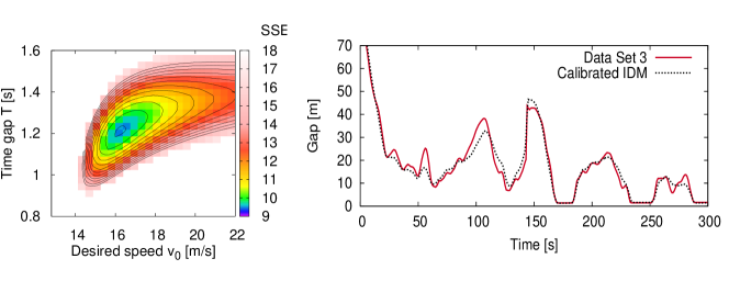
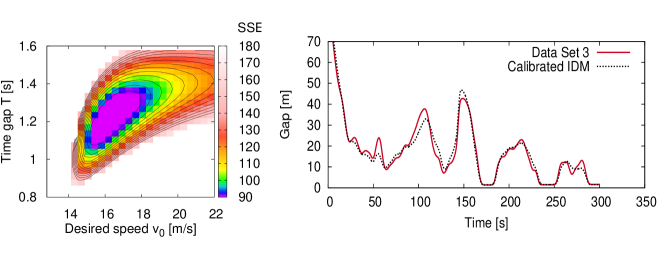
Fig. 7: Sensitivity analysis of the global calibration of the IDM (objective function (17)) to the xFCD Set 3 with respect to data properties. Top: Sampling interval $\Delta t=1\,\mathrm{s}$ instead of 0.1 s. Bottom: Gaussian kernel-based smoothing of the original set with a width $w2\,\mathrm{s}$.

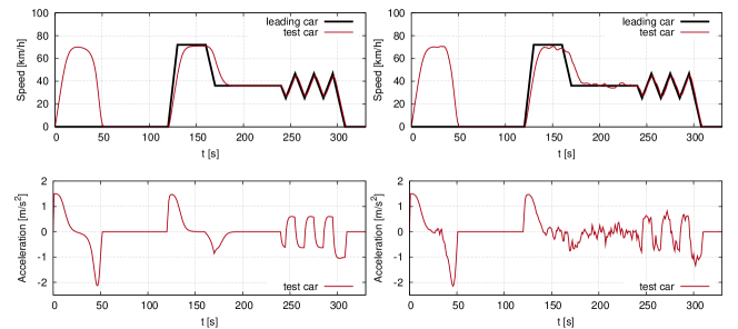
Fig. 8: virtual xFCD generated by an IDM vehicle ($v_{0}=20\,\mathrm{m/s}$, $T=1\,\mathrm{s}$, $s_{0}=2\,\mathrm{m}$, $a=1.5\,\mathrm{m/s^{2}}$, $b=2\,\mathrm{m/s^{2}}$) without noise (left), and with serially correlated noise induced – via a model of human drivers [32] – by estimation errors of the inverse time-to-collision $r=\Delta v/s$ (standard deviation 10 %, correlation time 10 s) (right). The speed profile of the leading vehicle (thick solid line) and the initial gap and speed of the follower are prescribed.

4.2 Effects of Data Smoothing

For the sensitivity analysis with respect to data smoothing, we start with the original data (sampling interval 0.1 s), apply Gaussian kernel-based averaging of variable smoothing width $w$ on the primary quantities (gap and speed), and calculate the rest of the variables by Eq. (4). Table 2 and Fig. 7 show that, up to a smoothing width $w=1\,\mathrm{s}$, the estimates obtained by global calibration and the fitness landscape of the objective functions (including correlations and covariances) remains essentially unchanged. As expected, the fit quality increases with $w$ (while it deteriorates with the sampling interval for intervals above 0.5 s).

As a further test to confirm this result, and also to test for a bias of the parameter estimate caused by noise, we calibrate the IDM on virtual xFCD generated by the same model with additional serially correlated acceleration noise (Figure 8) and repeat the calibration for several realizations of the noisy trajectory. We find no significant bias with the exception of the acceleration parameter $a$ for local calibration, which is systematically estimated too low. The observed variations of the estimates, however, are higher than indicated by the optimization software confirming the influence of serial correlations. Finally, data smoothing did not improve the result significantly.

We conclude that, in spite of possible artifacts due to numerical differentiation, no data smoothing is necessary when performing a global calibration on xFC data. While first evidence indicates that this is also true for the NGSIM data generally containing larger errors (cf. Section 3.2), a systematic investigation remains to be done.

5 Investigations on the Parameter Space

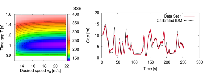
Fig. 9: Global calibration of the IDM to xFCD Set 1 with respect to the relative gaps.

5.1 Data completeness and parameter orthogonality

When calibrating the IDM to the xFCD Set 3 (Fig 1), we always obtain smooth objective functions with a unique global minimum. This also is true for many other time-continuous models and some time-discrete models. However, Fig. 9 shows that things are different for xFCD Set 1. The contour plot of the objective landscape (left part of this figure) shows that the minimum is indifferent with respect to the desired speed. The same is true for the deceleration parameter $b$. In fact, the unconstrained minimization yields $v_{0}\approx 1000\,\mathrm{km/h}$ (i.e., de facto, unbounded) and $b=6.9\,\mathrm{m/s}$ which is unrealistically high as well. Qualitatively, we obtain the same results for other models containing the desired speed and/or the approaching deceleration as (combinations of) model parameters as in Gipps’ model. The reason lies in the data set containing neither free-flow nor approaching situations but only congested and stopped traffic.

In such a situation, it is favorable to use a model which is parameter orthogonal meaning that different identifiable driving situations (such as freely accelerating, cruising, approaching, following or standing) are represented by different parameters, ideally one for each situation. If certain situations are not included in the data, the corresponding parameters are unobservable and must not be calibrated. Instead, we fix them to values which lie in the corresponding indifferent regimes. The contour plot of Fig. 9 indicates, that the desired speed lies in the indifferent regime if $v_{0}>20$. Parameter orthogonal model allows to identify such regimes, a priory, by the data. For the IDM, for example, it is safe to assume

$$v_{0}=2\max\limits_{i}\left(v_{i}\right),\quad b=-2\max\limits_{i}\left(-\dot{v}_{i}\right)$$ (23)

if the data contain no free-flow and no approaching situations, respectively. Calibrating the remaining IDM parameters with respect to relative gaps on xFCD Set 1, we obtain $T=1.02\,\mathrm{s}$, $s_{0}=2.26\,\mathrm{m}$, and $a=1.22\,\mathrm{m/s^{2}}$ while the unconstrained five-dimensional calibration yielded $T=1.03\,\mathrm{s}$, $s_{0}=2.25\,\mathrm{m}$, and $a=1.22\,\mathrm{m/s^{2}}$. We conclude that the values of the remaining parameters and the fit quality (the minimized SSE) do not change when restricting the calibration. Additionally, the restriction reduces the indicative estimation errors by about 10 %.

Notice that, since the objective functions deviate strongly from their local parabolic shape (see, e.g., Fig.4), parameter orthogonality does not necessarily mean that the correlation matrix of the indicative estimation errors (or, equivalently, the inverse Hessian of the objective function at the estimated values) is diagonal. Nevertheless, low correlations not exceeding absolute values of 0.5 indicate a good model quality. For the IDM, the correlation between $v_{0}$ and $T$ is often greater than 0.5 since the effects of increased desired speed are partially compensated for by an increased following time gap. However, all other cross correlations are generally below 0.5.

In order to apply (23), we need a systematic data-based procedure to distinguish the different regimes. We propose five regimes and following discrimination criteria:

• Cruising if the speed and the time gap are above data-driven limits $v_{c}$ and $T_{c}$, respectively, and the absolute acceleration is below a limit $a_{c}$,

• free acceleration if the time gap is above $T_{c}$, the acceleration above $a_{c}$, and the conditions for cruising are not fulfilled,

• approaching if $v>v_{l}$, the time gap $s/v>T_{c}$, and the kinematic deceleration $(v-v_{l})^{2}/(2s)>a_{c}$,

• essentially standing if the gap $s<s_{c}$,

• following if $T<T_{c}$ and none of the above conditions applies,

• and inconsistent behavior, otherwise.

Regime	xFCD Set 1	xFCD Set 3
cruising	0 %	5 %
free acceleration	16 %	8 %
approaching	2 %	3 %
standing	4 %	15 %
following	72 %	65 %
inconsistent	3 %	4 %

Table 4: driving regimes contained in the xFCD sets.

Table 4 shows the regime distribution for the two considered xFC data sets. As expected, Set 1 does not contain cruising episodes and describes approaching situations only 2 % of the time.

5.2 Model completeness

Not only data can be incomplete if they lack characteristic traffic situations but also models if they are not able to describe all situations. For example, car-following models in the stricter sense cannot describe free traffic flow. An example of such an incomplete model is the full velocity-difference model (FVDM) [22]. This model augments the optimal-velocity model [21] by a linear speed sensitivity term. It can be formulated as

$$\frac{{\rm d}v}{{\rm d}t}=a\left(\frac{v_{\rm opt}(s)-v}{v_{0}}\right)+\gamma(v_{l}-v).$$ (24)

Assuming an optimal-velocity function

$$v_{\rm opt}(s)=\max\left[0,\min\left(v_{0},\frac{s-s_{0}}{T}\right)\right],$$ (25)

its static model parameters $v_{0}$, $T$, and $s_{0}$ and the maximum acceleration $a$ have the same meaning as the corresponding IDM parameters. The IDM model parameter $b$ is replaced by the speed-difference sensitivity $\gamma$.

The incompleteness is caused by the last term describing a linear sensitivity to speed differences. Since this term does not depend on the gap, it describes interactions of an infinite range, i.e., in contrast to the OVM, the FVDM cannot describe free traffic flow [7].

parameter	OVM, Set 1	OVM, Set 3	FVDM, Set 1	FVDM, Set 3
desired speed $v_{0}[\mathrm{m/s}]$	170	14.0	12.8	14.1
desired time gap $T[\mathrm{s}]$	1.09	1.38	1.08	1.44
minimum gap $s_{0}[\mathrm{m}]$	2.75	2.86	2.76	1.52
maximum acceleration $a[\mathrm{m/s^{2}}]$	182	16.4	12.0	9.03
relative speed sensitivity $\gamma[\mathrm{s^{-1}}]$	-	-	0.08	0.65

Table 5: Global calibration of the optimal-velocity and full-velocity-difference models (24), (25) to the xFCD sets with respect to the relative gaps.

Table 5 shows that, as a consequence, the calibrated FVDM essentially reverts to the OVM if such situations arise. As a further consequence, the calibrated FVDM is nearly as unstable as the OVM and the acceleration parameter assumes unrealistically high values in order to compensate for the increased instability by a higher agility. This means, the FVDM is not only incomplete but also not parameter orthogonal. Finally, we notice that, due to the extreme values of the calibrated OVM acceleration parameter, the OVM vehicles follow their leader nearly statically at the optimal gap $s_{\rm opt}(v_{l})=s_{0}+v_{l}T$ (the inverse of the optimal velocity function) if the speed is below the desired speed.

6 Conclusions

Most other publications on calibrating car-following models focus on the fit quality. Most authors conclude that there is an unsurmountable barrier for the rms error (which, depending on the optimization measure, is of the order of 20 %) resulting in a stalemate when determining the “best” model. In this contribution, we have shown that there are other criteria for assessing model quality, namely completeness, robustness, parameter orthogonality, and intuitive parameters that are calibrated to plausible values. For example, in terms of the rms fitting error, the full-velocity difference model is only marginally worse than the IDM or Gipps’ model. Nevertheless, it is significantly inferior in terms of our proposed criteria.

Besides model quality, we also investigated the influence of the calibration method and data quality on the calibration result. It turned out that, generally, a global calibration based on the gaps is more reliable and robust compared to a local calibration or compared to a global calibration based on speeds or accelerations, in agreement with [29]. Concerning the data, we found that the common sampling rates of 10 Hz are unneccessarily high and that 1 Hz suffices. Furthermore, in contrast to intuition, smoothing the data had no significant influence on the calibration quality while data completeness, and also a minimum total time interval of the order of 300 s, and the absence of significant behavioural changes are crucial.

In a following contribution, we will investigate whether these results which are obtained for rather high-quality xFCD and for a very limited selection of NGSIM trajectory data will carry over to a systematic investigation of the noisier NGSIM trajectory data. Further research fields concern the influence of inter- and intra-driver variations. Regarding intra-driver variations, behavioural changes in anticipation of or after actions not contained in the models (such as lane changes) are highly relevant and deserve further investigation. It has been observed that different data sets can be described best by different models representing different driving styles. We plan to quantify this by proposing a model similarity matrix.

We conclude this contribution with some hints for performing a specific calibration task:

• Verify that the data do not describe traffic flow near a “tipping point” (e.g., at the verge of congestion or containing the onset of a traffic breakdown) which is unsuitable for calibration.

• Test the data for obvious behavioural changes in preparation for, or after, actions not desribed by the acceleration model, e.g., active or passive lane changes. Eliminate these time intervals or use a model including such actions.

• Select a model with intuitive parameters and plausible (published) values.

• Identify which parameters of a model are relevant for the traffic situations to be found in the data. Keep the other parameters fixed at published or plausible values.

• Restrict the remaining parameter space by a bounding box containing all plausible parameter combinations. At any stage of estimation, the space outside is off-limits.

• Take care to find a good initial guess. If in doubt, start with the published values.

• Check the resulting estimate for plausibility. Plot the fitness landscape around the estimate to verify that there is a global minimum inside the bounding box.

References

References

- [1] Y. Wang, M. Papageorgiou, A. Messmer, Real-time freeway traffic state estimation based on extended kalman filter: Adaptive capabilities and real data testing, Transportation Research Part A: Policy and Practice 42 (10) (2008) 1340–1358.
- [2] M. Treiber, A. Kesting, Validation of traffic flow models with respect to the spatiotemporal evolution of congested traffic patterns, Transportation Research Part C: Emerging Technologies 21 (1) (2012) 31–41.
- [3] E. Brockfeld, R. D. Kühne, P. Wagner, Calibration and validation of microscopic traffic flow models, Transportation Research Record 1876 (2004) 62–70.
- [4] V. Punzo, F. Simonelli, Analysis and comparision of microscopic flow models with real traffic microscopic data, Transportation Research Record 1934 (2005) 53–63.
- [5] A. Kesting, M. Treiber, Calibration of car-following models using floating car data, in: A. Schadschneider, T. Pöschel, R. Kühne, M. Schreckenberg, D. E. Wolf (Eds.), Traffic and Granular Flow ’07, Springer, Berlin, 2009, pp. 117–127.
-
[6]
A. Kesting, Microscopic modeling of human and automated driving: Towards
traffic-adaptive cruise control, Doctoral thesis, Technische Universität
Dresden, open access
http://nbn-resolving.de/urn:nbn:de:bsz:14-ds-1204804167720-57734 (2008). - [7] M. Treiber, A. Kesting, Traffic Flow Dynamics: Data, Models and Simulation, Springer, Berlin, 2013.
- [8] E. Brockfeld, P. Wagner, Validating microscopic traffic flow models, in: Intelligent Transportation Systems Conference, 2006. ITSC’06. IEEE, IEEE, 2006, pp. 1604–1608.
- [9] A. Kesting, M. Treiber, Calibrating car-following models by using trajectory data: Methodological study, Transportation Research Record 2088 (2008) 148–156.
- [10] S. Ossen, S. P. Hoogendoorn, Validity of trajectory-based calibration approach of car-following models in presence of measurement errors, Transportation Research Record 2088 (2008) 117–125.
- [11] C. Thiemann, M. Treiber, A. Kesting, Estimating acceleration and lane-changing dynamics from next generation simulation trajectory data, Transportation Research Record 2088 (2008) 90–101.
- [12] V. Punzo, M. Borzacchiello, B. Ciuffo, On the assessment of vehicle trajectory data accuracy and application to the next generation simulation (ngsim) program data, Transportation Research Part C: Emerging Technologies.
- [13] V. Punzo, B. Ciuffo, How parameters of microscopic traffic flow models relate to traffic dynamics in simulation: Implications for model calibration, Transportation Research Record 2124 (2009) 249–256.
- [14] S. Ossen, S. P. Hoogendoorn, B. G. Gorte, Inter-driver differences in car-following: A vehicle trajectory based study, Transportation Research Record 1965 (2007) 121–129.
- [15] A. Tordeux, S. Lassarre, M. Roussignol, An adaptive time gap car-following model, Transportation Research Part B: Methodological 44 (8-9) (2010) 1115–1131.
- [16] S. Ossen, S. Hoogendoorn, Heterogeneity in car-following behavior: Theory and empirics, Transportation Research Part C: Emerging Technologies 19 (2) (2011) 182–195.
- [17] V. Punzo, D. Formisano, V. Torrieri, Part 1: Traffic flow theory and car following: Nonstationary kalman filter for estimation of accurate and consistent car-following data, Transportation Research Record: Journal of the Transportation Research Board 1934 (-1) (2005) 1–12.
- [18] Y. Wang, M. Papageorgiou, Real-time freeway traffic state estimation based on extended kalman filter: a general approach, Transportation Research Part B: Methodological 39 (2) (2005) 141–167.
- [19] V. Punzo, B. Ciuffo, Sensitivity analysis of car-following models: Methodology and application, in: Transportation Research Board 90th Annual Meeting, DVD, Paper#11-2805, Transportation Research Board of the National Academies, Washington, D.C., 2011, pp. 1–18.
- [20] M. Treiber, A. Hennecke, D. Helbing, Congested traffic states in empirical observations and microscopic simulations, Physical Review E 62 (2000) 1805–1824.
- [21] M. Bando, K. Hasebe, A. Nakayama, A. Shibata, Y. Sugiyama, Structure stability of congestion in traffic dynamics, Japan Journal of Industrial and Applied Mathematics 11 (2) (1994) 203–223.
- [22] R. Jiang, Q. Wu, Z. Zhu, Full velocity difference model for a car-following theory, Physical Review E 64 (2001) 017101.
- [23] US Department of Transportation. NGSIM - Next Generation Simulation. 2012. http://ngsim-community.org/. Accessed August 14, 2012.
- [24] V. Punzo, M. Borzacchiello, B. Ciuffo, Estimation of vehicle trajectories from observed discrete positions and next-generation simulation program (ngsim) data, in: TRB 2009 Annual Meeting, 2009.
- [25] A. Kesting, M. Treiber, D. Helbing, Enhanced intelligent driver model to access the impact of driving strategies on traffic capacity, Philosophical Transactions of the Royal Society A 368 (2010) 4585–4605.
- [26] S. Hoogendoorn, R. Hoogendoorn, Calibration of microscopic traffic-flow models using multiple data sources, Philosophical Transactions of the Royal Society A: Mathematical, Physical and Engineering Sciences 368 (1928) (2010) 4497–4517.
- [27] B. Ciuffo, V. Punzo, V. Torrieri, Comparison of simulation-based and model-based calibrations of traffic-flow microsimulation models, Transportation Research Record: Journal of the Transportation Research Board 2088 (-1) (2008) 36–44.
-
[28]
M. Lourakis, levmar: Levenberg-marquardt nonlinear least squares algorithms in
C/C++, [web page]
http://www.ics.forth.gr/~lourakis/levmar/, [Accessed on 31 Jan. 2005.] (Jul. 2004). - [29] V. Punzo, F. Simonelli, Analysis and comparison of microscopic traffic flow models with real traffic microscopic data, Transportation Research Record: Journal of the Transportation Research Board 1934 (-1) (2005) 53–63.
- [30] P. G. Gipps, A behavioural car-following model for computer simulation, Transportation Research Part B: Methodological 15 (1981) 105–111.
- [31] G. F. Newell, A simplified car-following theory: a lower order model, Transportation Research Part B: Methodological 36 (3) (2002) 195–205.
- [32] M. Treiber, A. Kesting, D. Helbing, Delays, inaccuracies and anticipation in microscopic traffic models, Physica A 360 (2006) 71–88.