Cosmology in a certain vector-tensor theory of gravitation

Abstract

We study relevant cosmological topics in the framework of a certain vector-tensor theory of gravitation (hereafter VT). This theory is first compared with the so-called extended electromagnetism (EE). These theories have a notable resemblance and both explain the existence of a cosmological constant. It is shown that, in EE, a positive dark energy density requires a Lagrangian leading to quantum ghosts, whereas VT is free from these ghosts. On account of this fact, the remainder of the paper is devoted to study cosmology in the framework of VT. Initial conditions, at high redshift, are used to solve the evolution equations of all the VT scalar modes. In particular, a certain scalar mode characteristic of VT –which does not appear in general relativity (GR)– is chosen in such a way that it evolves separately. In other words, the scalar modes of the standard model based on GR do not affect the evolution of the VT characteristic mode; however, this scalar mode influences the evolution of the standard GR ones. Some well known suitable codes (CMBFAST and COSMOMC) have been modified to include our VT initial conditions and evolution equations, which are fully general. One of the resulting codes –based on standard statistical methods– has been used to fit VT predictions and observational evidences about both Ia supernovae and cosmic microwave background anisotropy. Seven free parameters are used in this fit. Six of them are often used in GR cosmology and the seventh one is characteristic of VT. From the statistical analysis it follows that VT seems to be advantageous against GR in order to explain cosmological observational evidences.

I Introduction

Extended electromagnetism (EE) was proposed in paper bm091 . The basic fields of this theory are the metric $g^{\mu\nu}$ and the electromagnetic field $A^{\mu}$. The fundamental symmetry is $A^{\mu}\rightarrow A^{\mu}+\nabla^{\mu}\Phi$, with $\nabla_{\mu}\nabla^{\mu}\Phi=0$; which is different from the standard U(1) gauge symmetry.

Some cosmological applications of EE were discussed in various papers (bm092, ; bm011, ; dal12, ). In Dale & Sáez dal12 , the variational formulation of EE was revisited, and the cosmological linear perturbations were studied by using the well known Bardeen formalism (bar80, ; huw97, ).

There is a vector-tensor (VT) theory of gravitation, studied in dal09 , which has a notable resemblance with EE. The post-Newtonian parametrized limit of VT is identical to that of general relativity (GR). Moreover, this theory was proved to be viable in bm093 (see below for more details). Here, the theories EE and VT are compared to conclude that, although they give the same results in cosmology, there are some problems with EE quantification. On account of these facts, our cosmological results are presented in the framework of VT.

The initial conditions for the evolution of scalar perturbations are taken in the radiation dominated era, at redshift $z\sim 10^{8}$, when the perturbations of cosmological interest are outside the effective horizon (see paper mb95 for details). By using these initial conditions, the linear equations satisfied by the scalar perturbations are numerically solved, and the cosmic microwave background (CMB) anisotropy is estimated. Since all the scalar perturbations are evolved from the radiation dominated era, it may be seen how metric perturbations gradually deviate from the GR ones. Deviations arises at some redshift to be numerically estimated, without a priori assumptions about its possible value.

There are well tested codes which are ready to do some calculations (evolution of scalar perturbations, CMB analysis, and so on) for standard cosmological models based on GR; e.g., CMBFAST (seza96, ) and CAMB (lew00, ). These codes may be modified to work in the framework of VT (or EE). In spite of the fact that CMBFAST is not currently maintained, its last version is good enough for us and, moreover, its equations are essentially written by using the Bardeen formalism in the version of mb95 , which is the same formalism used to study VT along this paper. By this reason, we may easily modify CMBFAST to describe cosmological evolution in VT. The necessary modifications –based on references bar80 , mb95 , and dal12 – are lengthy but straightforward. The code COSMOMC (lew02, ) has been also modified for statistical analysis in VT; namely, to fit theoretical predictions and observations by using a set of parameters (see next sections for details).

Our signature is (–,+,+,+). Greek (Latin) indices run from $0$ to $3$ (1 to 3). The symbol $\nabla$ ($\partial$) stands for a covariant (partial) derivative. The antisymmetric tensor $F_{\mu\nu}$ is defined by the relation $F_{\mu\nu}=\nabla_{\mu}A_{\nu}-\nabla_{\nu}A_{\mu}$, where $A^{\mu}$ is the vector field of the theory under consideration (EE or VT). Quantities $R_{\mu\nu}$, $R$, and $g$ are the covariant components of the Ricci tensor, the scalar curvature and the determinant of the matrix $g_{\mu\nu}$ formed by the covariant components of the metric, respectively. The gravitational constant is denoted $G$. Units are chosen in such a way that the speed of light is $c=1$. The scale factor is $a$. In flat universes, the present value of $a$ is arbitrary. We take a=1. The coordinate and conformal times are $t$ and $\tau$, respectively. Whatever quantity $D$ may be, $D_{B}$ stands for its background value and $\dot{D}$ is its derivative with respect to the conformal time.

This paper is structured as follows. In Sec. II, some general aspects of VT and EE and the cosmological background equations of both theories are presented and compared. In Sec. III, the evolution equations of all the VT cosmological scalar modes and the initial conditions necessary to their numerical integration are found. Numerical results are obtained with our modified versions of CMBFAST and COSMOMC. These results are analyzed in Sec. IV and, finally, Sec. V is a general discussion about methodology and conclusions.

II Basic equations of EE and VT. Background universe

The basic equations of EE may be derived from the action (dal12, ):

$$I=\int\left[\frac{R}{16\pi G}-\frac{1}{4}F^{\mu\nu}F_{\mu\nu}+\gamma(\nabla_{\mu}A^{\mu})^{2}+J^{\mu}A_{\mu}-\rho(1+\epsilon)\right]\,\sqrt{-g}\,d^{4}x\ ,$$ (1)

where $\gamma$ is a dimensionless arbitrary parameter, $J^{\mu}$ is the electrical current, $\rho$ is the conserved energy density of an isentropic perfect fluid, and $\epsilon$ is its internal energy density [see papers dal12 and haw99 for details].

From action (1), we have found two coupled field equations. The first equation is a generalization of the GR equation describing gravity. This equation may be written in the following form:

$$G^{\mu\nu}=8\pi G(T^{\mu\nu}_{GR}+T^{\mu\nu}_{EE})\ ,$$ (2)

where $G^{\mu\nu}$ is the Einstein tensor, $T^{\mu\nu}_{GR}$ is the energy momentum tensor of a fluid as it appears in GR, and the energy momentum tensor of the electromagnetic field –in EE theory– is $T^{\mu\nu}_{EE}$. The second equation is a generalization of Maxwell equation in curved space-time. This equation reads as follows:

$$\nabla^{\nu}F_{\mu\nu}=J_{\mu}+J^{{}^{A}}_{\mu}\ ,$$ (3)

where $J^{{}^{A}}_{\mu}=-2\gamma\nabla_{\mu}(\nabla\cdot A)$ –with $\nabla\cdot A=\nabla_{\mu}A^{\mu}$– plays the role of a new fictitious current. From this last equation one easily finds the relation

$$\nabla^{\mu}(J_{\mu}+J^{{}^{A}}_{\mu})=0$$ (4)

and, consequently, the total current $J_{\mu}+J^{{}^{A}}_{\mu}$ is conserved.

The energy momentum tensors $T^{\mu\nu}_{GR}$ and $T^{\mu\nu}_{EE}$ involved in Eqs.(2) are

$$T^{\mu\nu}_{GR}=(\mu+P)U^{\mu}U^{\nu}+Pg^{\mu\nu}$$ (5)

$$T^{\mu\nu}_{EE} = F^{\mu}_{\,\,\,\,\alpha}F^{\nu\alpha}-\frac{1}{4}g^{\mu\nu}F_{\alpha\beta}F^{\alpha\beta}$$ (6)

$$+2\gamma[\{A^{\alpha}\nabla_{\alpha}(\nabla\cdot A)+\frac{1}{2}(\nabla\cdot A)^{2}\}g^{\mu\nu}-A^{\mu}\nabla^{\nu}(\nabla\cdot A)-A^{\nu}\nabla^{\mu}(\nabla\cdot A)]\ .$$

The part of this last energy momentum tensor depending on $\gamma$ appears in EE but not in Einstein-Maxwell (E-M) theory. The two first terms of this tensor also appear in E-M.

In vector-tensor theories of gravitation, there are also two fields, the metric $g_{\mu\nu}$, and a four-vector $A^{\mu}$ which has nothing to do with the electromagnetic field. Various of these theories have been developed (see wil93 , wil06 and references cited there). They are based on the general action (wil93, ):

$$I = \int[R/16\pi G+\omega A_{\mu}A^{\mu}R+\eta R_{\mu\nu}A^{\mu}A^{\nu}-\varepsilon F_{\mu\nu}F^{\mu\nu}+\gamma\,\nabla_{\nu}A_{\mu}\nabla^{\nu}A^{\mu}$$ (7)

$$-\rho(1+\epsilon)]\sqrt{-g}\,d^{4}x\ ,$$

where $\omega$, $\eta$, $\varepsilon$, and $\gamma$ are arbitrary parameters. The tensor $F_{\mu\nu}$ –defined above– is not the electromagnetic one. In action (7), it is implicitly assumed that there are no couplings of $A_{\mu}$ with matter fields and electrical currents.

We are interest in the theory VT, which may be derived from the action (7) for $\omega=0$, and $\eta=\gamma$ (see dal09 ). With these parameters, the Lagrangian of Eq. (7) is easily proved to be equivalent to that involved in the following action (the difference is a total divergence):

$$I=\int\left[\frac{R}{16\pi G}+(\frac{\gamma}{2}-\varepsilon)F^{\mu\nu}F_{\mu\nu}+\gamma\,(\nabla_{\mu}A^{\mu})^{2}-\rho(1+\epsilon)\right]\,\sqrt{-g}\,d^{4}x\ .$$ (8)

A complete discussion about ghosts and unstable modes in VT was presented in section 3.1.3 of reference bm093 , where it was proved that there are no problems with this theory for $2\varepsilon-\gamma>0$. This condition is hereafter assumed.

Let us now compare actions (1) and (8). Action (8) does not contain the term $J^{\mu}A_{\mu}$ involved in Eq. (1), and the coefficient of $F^{\mu\nu}F_{\mu\nu}$ is arbitrary in action (8) whereas it takes on the value $-1/4$ in Eq. (1). These differences are consistent with the fact that EE is a theory of electromagnetism whereas VT is a theory of gravitation, in which, $A^{\mu}$ and $F_{\mu\nu}$ have nothing to do with electromagnetism.

The fundamental equations of VT are easily obtained from the action (8). They have the following form:

$$G^{\mu\nu}=8\pi G(T^{\mu\nu}_{GR}+T^{\mu\nu}_{VT})\ ,$$ (9)

$$2(2\varepsilon-\gamma)\nabla^{\nu}F_{\mu\nu}=J^{{}^{A}}_{\mu}\ ,$$ (10)

with

$$T^{\mu\nu}_{VT} = 2(2\varepsilon-\gamma)[F^{\mu}_{\,\,\,\,\alpha}F^{\nu\alpha}-\frac{1}{4}g^{\mu\nu}F_{\alpha\beta}F^{\alpha\beta}]$$ (11)

$$-2\gamma[\{A^{\alpha}\nabla_{\alpha}(\nabla\cdot A)+\frac{1}{2}(\nabla\cdot A)^{2}\}g^{\mu\nu}-A^{\mu}\nabla^{\nu}(\nabla\cdot A)-A^{\nu}\nabla^{\mu}(\nabla\cdot A)]\ .$$

From Eq. (10) one easily gets the relation

$$\nabla^{\mu}J^{{}^{A}}_{\mu}=0\ ,$$ (12)

which may be seen as the conservation law of the fictitious current $J^{{}^{A}}_{\mu}$ defined above.

Let us finally answer the following question: Why the last terms of Eqs. (6) and (11) have the same form but opposite signs?. The answer to this question may be found in a previous paper (dal12, ), where we presented an exhaustive variational formulation of EE based on the action (1). Some important aspects of this variational formulation are pointed out here, with the essential aim of answering the above question. Our variational method is described in haw99 (see section 3.3), where it is used to study the evolution of an isentropic fluid satisfying a certain conservation law. The same method may be easily generalized to deal with action (1), in which the vector field $A^{\mu}$, the fluid four-velocity $U^{\mu}$, and the metric $g_{\mu\nu}$, must be successively varied.

The field $A^{\mu}$ is first varied –for arbitrary $g_{\mu\nu}$ and $U^{\mu}$– to get Eqs. (3) and the conservation law (4), which may be rewritten as follows: $\partial_{\mu}[\sqrt{-g}(J^{\mu}+J^{A\mu})]=0$.

In a second step, only the four-velocity is varied, whereas the field $A^{\mu}$ is any arbitrary solution of Eqs. (3)–(4) for arbitrary metric. Then, the charge density $\rho_{q}$ is adjusted to keep the total current $J^{\mu}+J^{A\mu}$ conserved ($J^{\mu}=\rho_{q}U^{\mu}$). Thus, the following equation is obtained

$$(\mu+P)U^{\mu}\nabla_{\mu}U^{\nu}=-\nabla_{\mu}P(g^{\mu\nu}+U^{\mu}U^{\nu})+F^{\mu\nu}J_{\mu}+(\nabla^{\mu}J^{{}^{A}}_{\mu})A^{\nu}\ .$$ (13)

This equation was already derived in dal12 . See also haw99 for similar calculations in GR.

Finally, only the metric is varied, whereas the vector $A^{\mu}$ is fixed as in the second step, and vector $V^{\mu}$ satisfies Eq. (13) whatever $g^{\mu\nu}$ may be; hence, since density $\rho_{q}$ has been appropriately adjusted (see above), the conservation law $\partial_{\mu}[\sqrt{-g}(J^{\mu}+J^{A\mu})]=0$ is satisfied along the flow lines for arbitrary $g^{\mu\nu}$. Hence, $\sqrt{-g}(J^{\mu}+J^{A\mu})$ is unchanged when the metric is varied (see haw99 ); namely, we can write

$$\Delta_{g}(\sqrt{-g}J^{\mu})=-\Delta_{g}(\sqrt{-g}J^{{}^{A}\mu})\ ,$$ (14)

where $\Delta_{g}$ stands for a metric variation.

Equation (14) implies that the term $J^{\mu}A_{\mu}$ –involved in action (1)– is equivalent to $-J^{A\mu}A_{\mu}$ under the $\Delta_{g}$ variations necessary to get the energy-momentum tensor. Taking into account this fact, plus the identity $\nabla^{\mu}[A_{\mu}(\nabla\cdot A)]=(\nabla\cdot A)^{2}+A_{\mu}\nabla^{\mu}(\nabla\cdot A)$, and the definition of the fictitious current $J^{A\mu}$, it is easily proved that the Lagrangian densities $\gamma(\nabla_{\mu}A^{\mu})^{2}+J^{\mu}A_{\mu}$ and $-\gamma(\nabla_{\mu}A^{\mu})^{2}$ are fully equivalent under $g_{\mu\nu}$ variations (their difference is a total divergence); therefore, the energy-momentum tensors of EE and VT may be calculated from the Lagrangian densities $-\gamma(\nabla_{\mu}A^{\mu})^{2}$ and $\gamma(\nabla_{\mu}A^{\mu})^{2}$, respectively. Hence, the signs appearing in the last terms of Eqs. (6) and (11) must be opposite. This fact will play an important role later in this paper. It is a consequence of the conservation law (4).

Let us now consider a flat uncharged homogeneous and isotropic background universe with matter and radiation in both EE and VT. In this flat background, the metric has the Robertson-Walker form. Moreover, the following relations are satisfied: $A_{i}=0$ and $F_{\mu\nu}=0$ (dal12, ).

In EE, Eqs.(2), (5), and (6) lead to

$$3\frac{\dot{a}^{2}}{a^{2}}=8\pi Ga^{2}(\rho_{B}+\rho^{A}_{B})$$ (15)

$$-2\frac{\ddot{a}}{a}+\frac{\dot{a}^{2}}{a^{2}}=8\pi Ga^{2}(P_{B}+P^{A}_{B})$$ (16)

where $\rho_{B}$ and $P_{B}$ are the background energy density and pressure of the cosmological fluid (baryons, dark matter, massless neutrinos and radiation), and quantities $\rho^{A}_{B}$ and $P^{A}_{B}$ are associated to the part of the energy-momentum tensor (6) depending on $\gamma$. From this part, the following relation is easily obtained:

$$\rho^{A}_{B}=-P^{A}_{B}=-\gamma(\nabla\cdot A)_{B}^{2}\ .$$ (17)

Hence, constant $\gamma$ must be negative to have a positive energy density.

In VT, Eqs. (15) and (16) hold, but $\rho^{A}_{B}$ and $P^{A}_{B}$ must be defined by using the energy-momentum tensor (11); from which, one easily gets:

$$\rho^{A}_{B}=-P^{A}_{B}=\gamma(\nabla\cdot A)_{B}^{2}\ .$$ (18)

Therefore, constant $\gamma$ must be positive to have $\rho^{A}_{B}>0$.

We have shown that simple applications to cosmology fix the sign of $\gamma$ in both EE and VT. This sign is irrelevant in cosmology, but it is important in quantum field theory. On account of Eq. (1), a negative sign of the coefficient $\gamma$ would lead to quantum ghosts. Hence, we hereafter develop our cosmological estimations in the framework of VT (with positive $\gamma$). In this theory, apart from the positive constant $\gamma$, whose value is unknown. There is a second constant $\varepsilon$ in Eq. (8), which must satisfy the condition $\varepsilon>\frac{\gamma}{2}$, but the exact value of $\varepsilon$ keeps unknown.

Let us now study other background equations in VT. From Eq. (10) one easily gets:

$$\Xi_{B}\equiv(\nabla\cdot A)_{B}=-\frac{1}{a^{2}}[\dot{A}_{0B}+2\frac{\dot{a}}{a}A_{0B}]=constant\ ,$$ (19)

where $A_{0B}$ is the time component of $A_{\mu}$ in the background. Eq. (19) describes the evolution of this component. This equation may be numerically solved for appropriate initial conditions to get function $A_{0B}(\tau)$. From Eqs. (18) and (19) one easily concludes that, at zero order (in the background), the energy density of the field $A^{\mu}$ and its pressure have the same absolute value and opposite signs, which means that $\rho^{A}_{B}$ plays the role of dark energy with the vacuum equation of state $W=P^{A}_{B}/\rho^{A}_{B}=-1$.

For vacuum energy ($W=-1$) and a flat background, CMBFAST uses Eqs. (15) and (16) with $\rho^{A}_{B}=\rho_{v}$, where $\rho_{v}$ is the vacuum energy; hence, in order to modify CMBFAST for VT calculations, the CMBFAST background equations are valid, but the new Eq. (19) must be included. According to Eq. (18), in this new equation we set

$$\Xi_{B}=S_{gn}\Big{(}\frac{\rho_{v}}{\gamma}\Big{)}^{1/2}\ ,$$ (20)

where the value of $S_{gn}$ is either $+1$ or $-1$. The $S_{gn}$ value fixes the arbitrary sign of $\Xi_{B}$. In addition to $\rho_{v}$, we have the arbitrary parameters $\gamma$ and $S_{gn}$. The integration of the new background equation

$$\dot{A}_{0B}=-a^{2}\Xi_{B}-2\frac{\dot{a}}{a}A_{0B}$$ (21)

requires the initial value of $A_{0B}$, which is taken at the initial redshift $z_{in}=10^{8}$ (as it is done for any variable). At this high redshift, during the radiation dominated era, there are power law functions of $\tau$ satisfying the background field equations. In fact, it is easily verified that the following functions $a=\alpha\tau^{\zeta}$ and $A_{0B}=\beta\tau^{\delta}$ satisfy the above background field equations –in the radiation dominated era– for $\zeta=1$, $\delta=3$. Then, at $z_{in}$, one finds:

$$\tau_{in}=\Big{(}\frac{\dot{a}}{a}\Big{)}_{in}^{-1}\ ,\,\,\,\,\,\,(A_{0B})_{in}=-\frac{\Xi_{B}}{5(1+z_{in})^{2}}\Big{/}\Big{(}\frac{\dot{a}}{a}\Big{)}_{in}\ .$$ (22)

Since CMBFAST rightly calculates the initial value of $\dot{a}/a$, the value of $A_{0B}$ at $z_{in}$ is not a free parameter. It is given in terms of $\rho_{v}$, $S_{gn}$ and $\gamma$ by Eqs. (20) and (22).

After proving that $\Xi_{B}$ and $A_{0B}$ are both proportional to $S_{gn}\gamma^{-1/2}$ [see Eqs. (20) – (22)], the background equations of VT might be easily solved for $\gamma=1$, $S_{gn}=+1$, and for appropriate amounts of baryons, dark matter, and photons –similar calculations were done by Dale & Sáez dal12 in EE– nevertheless, massless neutrinos would require a more complicated treatment. These neutrinos are taken into account in CMBFAST and also in our modification of this code, in which we include the VT parameters $\gamma$ and $S_{gn}$, the VT background equation (21) and, the new initial condition for $A_{0B}$ [see Eq. (22)]. Any other aspect of the CMBFAST background evolution is not altered at all.

III Cosmological scalar modes and initial conditions

There are no tensor modes associated to the vector field $A^{\mu}$ and, consequently, the evolution of tensor cosmological perturbations (primordial gravitational waves) is identical in GR and VT.

The vector modes involved in GR decrease as a result of expansion (mor07, ); hence, they are expected to be negligible at redshifts close to recombination and decoupling. Since significant vector modes might produce interesting effects (mor07, ; mor08, ) at these low redshifts, it is interesting the study of vector-tensor theories, which include the vector modes of GR plus an additional one associated to the vector field $A^{\mu}$. The field equations –of the vector-tensor theory– would couple all these modes which could evolve in an appropriate way justifying the existence of non negligible vector modes at redshifts close to $1000$. The study of vector modes in VT and also in other vector-tensor theories of gravitation is in progress.

Since the effects of vector and tensor modes on the CMB are expected to be small, this section is devoted to the study of scalar perturbations in the framework of VT.

The code CMBFAST solves the evolution equations of the scalar modes in GR cosmologies. In the flat case, these equations are written in terms of a certain set of scalar modes, whose initial values –at redshift $z=10^{8}$– are appropriately obtained (mb95, ). Calculations are performed in the synchronous gauge. In order to modify CMBFAST in the simplest way -for applications to VT– the gauge and the scalar modes used in this code must be maintained, and a new scalar mode associated to $A^{\mu}$ must be added. New terms depending on the new mode modify the CMBFAST equations (standard cosmology), and a new equation for the evolution of the $A^{\mu}$ mode must be also added. Finally, the initial values of all the coupled modes must be calculated at the chosen initial redshift.

For a standard flat cosmological background in GR, the formalism described in bar80 involves the scalar perturbations associated to the metric, the four-velocity, and the energy-momentum tensor of a cosmological fluid. These perturbations are expanded in terms of scalar harmonics as follows:

$$g_{00}=-a^{2}(1+2\tilde{A}Q^{(0)}),\,\,\,\,g_{0i}=-a^{2}\tilde{B}^{(0)}Q^{(0)}_{i},\,\,\,\,$$

$$g_{ij}=a^{2}[(1+2H_{L}Q^{(0)})\delta_{ij}+2H_{T}^{(0)}Q_{ij}^{(0)}]$$

$$U_{i}=av^{(0)}Q^{(0)}_{i},\,\,\,\,\rho=\rho_{B}(1+\delta Q^{(0)})$$

$$T_{ij}=P_{B}(1+\pi_{L}Q^{(0)})\delta_{ij}+P_{B}\pi_{T}^{(0)}Q_{ij}^{(0)}\ ,$$ (23)

where function $Q^{(0)}=\exp({i\vec{k}\cdot\vec{r}})$ is a plane wave, $Q^{(0)}_{i}=(-1/k)\partial_{i}Q^{(0)}$, and $Q_{ij}^{(0)}=k^{-2}\partial_{j}\partial_{i}Q^{(0)}+(1/3)\delta_{ij}Q^{(0)}$. The scalar modes $\tilde{A}$, $\tilde{B}^{(0)}$, $H_{L}$, $H_{T}^{(0)}$, $v^{(0)}$,$\delta$, $\pi_{L}$ and $\pi_{T}^{(0)}$ are functions of $k$ (wavenumber) and $\tau$. Any other quantity as, e.g., $U_{0}$ and $T_{0i}$, may be easily written in terms of these modes.

The synchronous gauge is fixed by the conditions $\tilde{A}=\tilde{B}^{(0)}=0$. In this gauge, the modes used in CMBFAST are those defined in Ma & Bertschinger mb95 . These modes are related to the Bardeen ones as follows: $h=6H_{L}$, $\eta=-H_{L}-H_{T}^{(0)}/3$, $\theta=kv^{(0)}$, $\sigma=2P_{B}\pi_{T}^{(0)}/3(\rho_{B}+P_{B})$. The same mode $\delta$ associated to the density contrast is used in paper bar80 and also in reference mb95 and, finally, $\pi_{L}$ is not directly used since it is related to $\delta$ by means of the equation of state, e.g., for adiabatic perturbations, the relation $\pi_{L}=(\rho_{B}/P_{B})(dP_{B}/d\rho_{B})\delta$ is satisfied. In addition to the CMBFAST scalar modes, a new one is necessary due to the existence of $A^{\mu}$. It is easily verified that the mode $\Xi^{(0)}$ defined by the equation

$$\nabla\cdot A=\Xi_{B}(1+\Xi^{(0)}Q^{(0)})\ ,$$ (24)

is the most appropriate to write the $A^{\mu}$ field equations in the simplest and most operating way. These equations reduces to (dal12, ):

$$\ddot{\Xi}^{(0)}+2\frac{\dot{a}}{a}\dot{\Xi}^{(0)}+k^{2}\Xi^{(0)}=0\ .$$ (25)

This second order differential equation does not involve the CMBFAST modes associated to the metric and the cosmological fluids. Apart from the mode $\Xi^{(0)}$, it only involves background functions as $\dot{a}/a$ and the wavenumber.

Eq. (25) is equivalent to the following system of linear differential equations

$$\dot{\Xi}^{(0)}=\xi^{(0)}$$ (26)

$$\dot{\xi}^{(0)}=-2\frac{\dot{a}}{a}\xi^{(0)}-k^{2}\Xi^{(0)}\,$$ (27)

which have been included in CMBFAST to be solved by using the initial values of $\Xi^{(0)}$ and $\xi^{(0)}$ derived below.

In the chosen gauge, Eqs. (5), (9), and (11) lead to the following linearized equations for the evolution of the scalar modes $h$ and $\eta$:

$$k^{2}\eta-\frac{1}{2}\frac{\dot{a}}{a}\dot{h}=4\pi G[-a^{2}\rho_{B}\delta-2\gamma\Xi_{B}(a^{2}\Xi_{B}\Xi^{(0)}+A_{0B}\xi^{(0)})]$$ (28)

$$k^{2}\dot{\eta}=4\pi G[a^{2}(\rho_{B}+P_{B})\theta+2\gamma k^{2}A_{0B}\Xi_{B}\Xi^{(0)}]$$ (29)

$$\ddot{h}+2\frac{\dot{a}}{a}\dot{h}-2k^{2}\eta=-24\pi G[a^{2}P_{B}\pi_{L}-2\gamma\Xi_{B}(a^{2}\Xi_{B}\Xi^{(0)}-A_{0B}\xi^{(0)})]$$ (30)

$$\ddot{h}+6\ddot{\eta}+2\frac{\dot{a}}{a}(\dot{h}+6\dot{\eta})-2k^{2}\eta=-24\pi Ga^{2}(\rho_{B}+P_{B})\sigma\ .$$ (31)

If the terms involving $\gamma$ are canceled, the equations of standard GR cosmology labeled (21a)–(21d) in Ma & Bertschinger mb95 are recovered. These terms –appearing only in VT cosmology– have been included in CMBFAST. Since $A_{0B}$ and $\Xi_{B}$ are proportional to $S_{gn}\gamma^{-1/2}$, it is obvious that the three VT terms are independent of both $S_{gn}$ and $\gamma$. The values taken by these terms depend on the initial values of $\Xi^{(0)}$ and $\xi^{0}=\dot{\Xi}^{(0)}$.

We assume that the universe contains baryons, photons, massless neutrinos, and dark matter. The energy momentum tensor of all these components is $T^{\mu\nu}_{GR}$. Dark energy is due to the field $A^{\mu}(\tau)$. The background energy density of this field is constant and its equation of state is $W=-1$. There are dark energy fluctuations, which have been taken into account to obtain Eqs. (28) – (31) by using the first order approximation of $T^{\mu\nu}_{VT}$.

By using Eqs. (10) and (12, it may be easily proved that the covariant divergence $\nabla_{\mu}T^{\mu\nu}_{VT}$ vanishes (see also wil93 ). Hence, according to Eq. (9), the energy-momentum conservation law $\nabla_{\alpha}T^{\alpha\beta}_{GR}=0$ is satisfied, as it occurs in the standard cosmological model based on GR. Therefore, the variables $\delta$, $\theta$, and $\sigma$ corresponding to each particle distribution obey the same equations as in standard GR cosmology and, consequently, we can write (see Eqs. (92) in paper mb95 ):

$$\dot{\delta}_{\gamma}+\frac{4}{3}\theta_{\gamma}+\frac{2}{3}\dot{h}=0,\,\,\,\,\dot{\theta}_{\gamma}-\frac{1}{4}k^{2}\delta_{\gamma}=0,\,\,\,\,$$

$$\dot{\delta}_{\nu}+\frac{4}{3}\theta_{\nu}+\frac{2}{3}\dot{h}=0,\,\,\,\,\dot{\theta}_{\nu}-\frac{1}{4}k^{2}(\delta_{\nu}-4\sigma_{\nu})=0,\,\,\,\,$$

$$\dot{\sigma}_{\nu}-\frac{2}{15}(2\theta_{\nu}+\dot{h}+6\dot{\eta})=0\ ,$$ (32)

where the indices $\gamma$ and $\nu$ make reference to photons and massless neutrinos, respectively. The treatment of the interaction between photons and baryons (including reionization) is also identical to that described by Ma & Bertschinger mb95 and implemented in CMBFAST. Finally, from Eqs. (28)– (31) and the background field equations, one easily finds the following differential equation:

$$\tau^{2}\ddot{h}+\tau\dot{h}+6\delta+32\pi G\gamma\tau^{2}(2\Xi_{B}A_{0B}\xi^{(0)}-a^{2}\Xi_{B}^{2}\Xi^{(0)})=0\ ,$$ (33)

where $\delta=(1-R_{\nu})\delta_{\gamma}+R_{\nu}\delta_{\nu}$, with $R_{\nu}=\rho_{\nu B}/(\rho_{\nu B}+\rho_{\gamma B})$. Of course, this last equation is satisfied in the radiation dominated era, where initial conditions are obtained. It generalizes the first of Eqs. (92) in paper mb95 . We have already found all the equations necessary to fix the initial conditions for integrations in VT cosmology. Therefore, let us now estimate the initial values of all the scalar modes at $z=10^{8}$. Our method to look for these values is similar to that described in Ma & Bertschinger mb95 for the CMBFAST modes, but it has been extended to take into account the new functions $\Xi^{(0)}$ and $\xi^{0}$. It is assumed that, in the radiation dominated era, any mode $X$ may be expanded in the form

$$X=\sum_{n,m}\beta_{nm}k^{n}\tau^{m}\ ,$$ (34)

where the values taken by the integer numbers $n$ and $m$ must be fixed for each $X$. The smallness of $k\tau$ for cosmological scales, the existence of growing and decaying terms in Eq. (34), and other considerations allow us to determine the n and m values being relevant for each mode. We begin with $\Xi^{(0)}$ and $\xi^{(0)}$.

For small enough scales ($k<<1$), the term proportional to $k^{2}$ in Eq. (25) may be neglected. Thus, this equation reduces to $\ddot{\Xi}^{(0)}+2\frac{\dot{a}}{a}\dot{\Xi}^{(0)}=0$. The solution of this equation is $\xi^{(0)}=\dot{\Xi}^{(0)}\propto a^{-2}\propto\tau^{-2}$. In order to obtain these last relations, it has been taken into account that the equation $a=\alpha\tau$ is satisfied in the radiation dominated era. A new integration leads to $\Xi^{(0)}=\tilde{D}_{1}+\tilde{D}_{2}\tau^{-1}$, where $\tilde{D}_{1}$ and $\tilde{D}_{2}$ are constants of integration. If the term involving $k^{2}$ is not neglected, Eq. (25) has the following approximating solution:

$$\Xi^{(0)}=D_{1}k^{n}\Big{[}1-\frac{1}{6}k^{2}\tau^{2}+\frac{1}{120}k^{4}\tau^{4}+...\Big{]}\ .$$ (35)

which is valid for values of $k\tau$ much smaller than unity. During a part of the radiation dominated era, including the time corresponding to redshift $z=10^{8}$, all the cosmological scales are outside the effective horizon and $k\tau$ is small enough to guarantee the validity of Eq. (35). In this equation, the terms of the form $k^{n+2}\tau^{m+2}$ may be neglected against the terms $k^{n}\tau^{m}$, which are much greater due to the smallness of $k\tau$. Taking into account this fact and Eq. (35), one easily finds the following values of $\Xi^{(0)}$ and $\dot{\Xi}^{(0)}$,

$$\Xi^{(0)}=D_{1}k^{n}\ ,\,\,\,\,\,\,\,\,\,\,\,\,\,\,\,\,\xi^{(0)}=\dot{\Xi}^{(0)}=0\ .$$ (36)

These values correspond to the largest term of the series (35) giving $\Xi^{(0)}$. Since they do not depend on $\tau$ during the part of the radiation dominated era mentioned above, the initial values of $\Xi^{(0)}$ and $\xi^{(0)}$, at $z=10^{8}$, are $\Xi^{(0)}_{in}=D_{1}k^{n}$ and $\xi^{(0)}_{in}=0$. We see that the initial conditions for the scalar modes characteristic of VT only depend on the parameter $D_{1}$ and, consequently, any possible new effect due to cosmological scalar modes appearing in VT –but not in GR– depends on the value of this parameter, which plays the role of a normalization constant. Since final results depend on $D_{1}$, comparisons with observations should lead to an estimate of this constant.

Let us now look for the initial conditions corresponding to the remaining variables to be evolved. Our method is analogous to that used in paper mb95 . First of all, the terms proportional to $k^{2}$ are neglected in Eq. (32); thus –as in standard cosmology– the following relations are found $\theta_{\nu}=\theta_{\gamma}=0$ and $\delta_{\nu}=\delta_{\gamma}=-(2/3)h$; hence

$$\delta=-(2/3)h$$ (37)

and

$$\theta\equiv(1-R_{\nu})\theta_{\gamma}+R_{\nu}\theta_{\nu}=0\ .$$ (38)

The second time derivative of Eq. (33) with respect to $\tau$ is calculated, and taking into account Eq. (37), the following relation is easily obtained:

$$\tau h^{(4)}+5h^{(3)}+32\pi G\gamma\tau^{-1}\ddot{\mu}=0\ ,$$ (39)

where

$$\mu=\tau^{2}(2\Xi_{B}A_{0B}\xi^{(0)}-a^{2}\Xi_{B}^{2}\Xi^{(0)})\ .$$ (40)

Taking into account the relations $A_{0B}\tau^{-3}=(A_{0B})_{in}\tau^{-3}_{in}$, $a\tau^{-1}=a_{in}\tau^{-1}_{in}$, plus Eqs. (20), (22), and (36), quantity $\ddot{\mu}$ may be easily calculated and replaced into Eq. (39) to get

$$\tau h^{(4)}+5h^{(3)}=\frac{384\pi GD_{1}\rho_{v}}{(1+z_{in})^{2}}\Big{(}\frac{\dot{a}}{a}\Big{)}_{in}k^{n}\tau$$ (41)

If the second order derivative of this equation –with respect to $\tau$– is calculated, the following equation is found:

$$\tau h^{(6)}+7h^{(5)}=0\ ,$$ (42)

where $h^{(6)}$ and $h^{(5)}$ stand for the sixth and fifth order derivatives of function $h$ with respect to $\tau$. Only the mode $h$ is involved in this equation. The sixth order differential equation (42) may be easily integrated. The solution is a linear combination of the powers $\tau^{-2}$, $\tau^{0}$, $\tau$, $\tau^{2}$, $\tau^{3}$, and $\tau^{4}$. The powers $\tau^{3}$ and $\tau^{4}$ do not appear in GR cosmology, where the equation to be solved has the form $\tau h^{(4)}+5h^{(3)}=0$ (see paper mb95 ).

By using the same arguments as in Ma & Bertschinger mb95 for the powers $\tau^{-2}$, $\tau^{0}$, $\tau$, $\tau^{2}$, but taking into account the new dependence in $\tau^{3}$, and $\tau^{4}$, we write

$$h(k,\tau)=C_{2}(k\tau)^{2}+C_{3}(k\tau)^{3}+C_{4}(k\tau)^{4}\ .$$ (43)

Thus, the initial condition of GR cosmology is recovered for $C_{3}=C_{4}=0$. For appropriate values of $C_{3}$ and $C_{4}$, the second and third terms of the right hand side of Eq. (43) might account for small deviations with respect to GR cosmology, which could be compatible with observations. By using Eq. (43), it is easily seen that, whatever $k$ and $\tau$ may be, Eq. (41) is identically satisfied for $n=4$,

$$C_{3}=0\ ,\,\,\,\,\,\,C_{4}=\frac{8\pi GD_{1}\rho_{v}}{3(1+z_{in})^{2}}\Big{(}\frac{\dot{a}}{a}\Big{)}_{in}^{2}\ .$$ (44)

Therefore, from Eqs. (43) and (44), it follows that, to lowest order in $k\tau$, function $h(k,\tau)$ involves two normalization constants $C_{2}$ and $D_{1}$. Constant $C_{2}$ also appears in standard GR cosmology, whereas $D_{1}$ is a new independent normalization constant. Standard cosmology is recovered for $D_{1}=0$ ($C_{4}=0$). For appropriate $D_{1}$ values, the term $C_{4}(k\tau)^{4}$ may be non negligible and, consequently, it could lead to deviations from standard cosmology, which might help to explain current observations better.

From Eqs. (29), (38), plus Eq. (36) with $n=4$, one easily finds

$$\dot{\eta}=-\frac{8\pi GD_{1}\rho_{v}}{5(1+z_{in})^{2}}\Big{(}\frac{\dot{a}}{a}\Big{)}_{in}^{2}k^{4}\tau^{3}\ .$$ (45)

A simple integration leads to

$$\eta=2C_{2}-\frac{3}{20}C_{4}k^{4}\tau^{4}\ .$$ (46)

Only the first term of the right hand side of this last equation arises in standard cosmology. The second term may be neglected –to lowest order in $k\tau$– since it involves a very small factor of the form $k^{4}\tau^{4}$. Hence, our approximation leads to $\dot{\eta}=0$. Since $\theta$ also vanishes, the last of Eqs. (32) reduces to $\dot{\sigma}_{\nu}=-\frac{2}{15}\dot{h}$.

The initial conditions to lowest order in $k\tau$ are summarized as follows:

$$\delta_{\gamma}=\delta_{\nu}=\frac{4}{3}\delta_{b}=\frac{4}{3}\delta_{c}=-\frac{2}{3}h,\,\,\,\,h=C_{2}(k\tau)^{2}+C_{4}(k\tau)^{4},$$

$$\theta_{\gamma}=\theta_{\nu}=\theta_{b}=\theta_{c}=0,\,\,\,\,\dot{\eta}=0,\,\,\,\,\dot{\sigma}_{\nu}=-\frac{2}{15}\dot{h}\ ,$$ (47)

where indices ${b}$ and ${c}$ stand for baryons and cold dark matter, respectively, and constant $C_{4}$ is given by Eq. (44). The term $C_{4}(k\tau)^{4}$ is not neglected in the formula for $h$ since quantity $k^{2}\tau^{2}$ is small, but constant $C_{4}$ may be greater than $C_{2}$.

Let us now combine Eqs. (32) –without neglecting the terms involving quantity $k^{2}$– to go beyond the lowest order in $k\tau$. A lengthy but straightforward calculation leads to:

$$\theta_{\gamma}=\theta_{b}=-\frac{1}{18}C_{2}k^{4}\tau^{3}-\frac{1}{30}C_{4}k^{6}\tau^{5},\,\,\,\,\theta_{\nu}=-\frac{23+4R_{\nu}}{18(15+4R_{\nu})}C_{2}k^{4}\tau^{3}-\frac{1}{30}C_{4}k^{6}\tau^{5}$$

$$\sigma_{\nu}=\frac{4}{3(15+4R_{\nu})}C_{2}k^{2}\tau^{2},\,\,\,\,\eta=\Big{[}2-\frac{5+4R_{\nu}}{6(15+4R_{\nu})}(k\tau)^{2}\Big{]}C_{2}\ .$$ (48)

Quantities $\delta_{\gamma}$, $\delta_{\nu}$, $\delta_{b}$, $\delta_{c}$, $h$, and $\theta_{c}$ have the same form as in Eq. (47). It is due to the fact that the new terms arising beyond the lowest order approximation in $k\tau$ are negligible. In the case $C_{4}=0$, Eqs. (48) reduce to the equations (96) derived by mb95 in the framework of the standard cosmological model. Differences are due to the terms involving the $C_{4}$ (equivalently $D_{1}$) normalization constant.

IV Numerical results

All the calculations are performed under the following basic assumptions: the background is flat, perturbations are adiabatic, the lensing effect is not considered, there are no massive neutrinos, the equation of state of the dark energy is $P=W\rho$ with $W=-1$, vector and tensor modes are negligible, the mean CMB temperature is $T_{CMB}=2.726$, the effective number of relativistic species is $3.046$, and the total number of effectively massless degrees of freedom is $g_{*}=10.75$.

Statistical methods (Markov chains) are used to fit the theoretical predictions (based on the above basic assumptions) to current observational evidences about high redshift Ia supernovae (SNe Ia) luminosity and CMB temperature anisotropy. In GR (VT), the fit is based on six (seven) parameters. Numerical calculations have been carried out by using modifications of the well known codes CMBFAST and COSMOMC. The new codes are hereafter called VT-CMBFAST and VT-COSMOMC. These tools have been designed for VT applications. The code VT-CMBFAST includes the equations and initial conditions obtained in Secs. II and III, which are necessary to describe both the VT background and the scalar modes. The original CMBFAST code uses the same formalism as in previous sections, which makes it easy to perform the modifications necessary to include new elements characteristic of VT. Since the code CAMB uses other formalism, we have preferred the modification of CMBFAST for VT cosmological studies. Although the original version of COSMOMC uses the code CAMB for the numerical estimation of CMB spectra and other quantities, we have designed the version VT-COSMOMC (for calculations in the framework of VT), which uses VT-CMBFAST instead of CAMB.

Table 1: Values of the fitted cosmological parameters. BF stands for best fit, and the marginalized lower and upper limits of each parameter, at $2\sigma$ (95 %) confidence, are listed in the L2 and U2 cases, respectively.

THEORY	CASE	$D_{1}\times 10^{-8}$	$\Omega_{b}h^{2}$	$\Omega_{DM}h^{2}$	$\tau$	$n_{s}$	$\log[10^{10}A_{s}]$	$\theta$
GR	BF	0.0	0.0223	0.112	0.0836	0.962	3.067	1.039
GR	L2	0.0	0.0207	0.096	0.0460	0.920	2.967	1.030
GR	U2	0.0	0.0237	0.124	0.1285	1.000	3.168	1.047
VT	BF	0.203	0.0224	0.112	0.0866	0.963	3.074	1.039
VT	L2	-5.314	0.0189	0.082	0.0103	0.878	2.871	1.022
VT	U2	5.320	0.02801	0.137	0.0203	1.119	3.324	1.054

First of all, with the basic assumptions, the observational data and the new codes mentioned in the first paragraphs of this section, we have found the best fit in the framework of GR ($D_{1}=0$). The six parameters used to fit predictions and observations are $\Omega_{b}h^{2}$, $\Omega_{DM}h^{2}$, $\tau$, $n_{s}$, $\log[10^{10}A_{s}]$, and $\theta$, where $\Omega_{b}$ and $\Omega_{DM}$ are the density parameters of baryons and dark matter, respectively, $h$ is the reduced Hubble constant, $\tau$ is the reionization optical depth, $n_{s}$ is the spectral index of the power spectrum of scalar modes, and $A_{s}$ is the normalization constant of the same spectrum whose form is $P(k)=A_{s}k^{n_{s}}$, finally, the parameter $\theta$ is defined by the relation $\theta\times 10^{-2}=d_{A}(z_{*})/r_{s}(z_{*})$, where $d_{A}(z_{*})$ is the angular diameter distance at decoupling redshift $z_{*}$, and $r_{s}(z_{*})$ is the sound horizon at the same redshift. The resulting values of the above six parameters corresponding to our best fit in GR are given in the first row of Table 1. These values are compatible with those of Table 8 in jar11 , which were obtained from the Wilkinson microwave anisotropy probe seven (WMAP7) years data. For each parameter, the second (third) row of this Table defines the lower (upper) limit of an interval, which contains the true value of the chosen parameter, at $95$ % confidence, in the marginalized case; namely, if the remaining five parameters are chosen to be those of the first row of Table 1(best fit).

We have used VT–CMBFAST to find the following CMB angular power spectra: (i) the $C^{TT}_{\ell}$ ($C^{EE}_{\ell}$) coefficients measuring CMB temperature (E-polarization) correlations at angular scales $\alpha=\pi/\ell$ with $\ell<2100$, and (ii) the parameters $C^{ET}_{\ell}$ giving the cross correlations between temperature and E-polarization for the same scales. The resulting $C^{TT}_{\ell}$ quantities corresponding to various cases are presented in Fig. 1. In all these cases, the values of the six parameters used in our previous fit (first row of Table 1) have been fixed, whereas parameter $D_{1}$ has been varied. For $D_{1}=0$ (solid line) the angular power spectrum corresponds to our GR best fit (first row of Table 1).

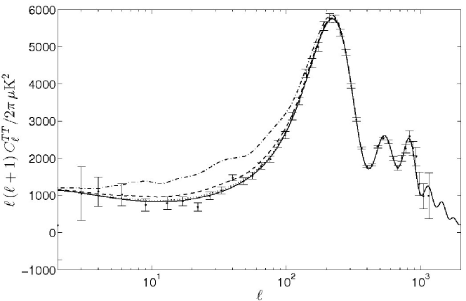
Figure 1: CMB temperature angular power spectra in terms of $\ell$. Solid, dotted, dashed, and dotted-dashed lines correspond to $D_{1}=0$, $D_{1}=2\times 10^{8}$, $D_{1}=4\times 10^{8}$, and $D_{1}=8\times 10^{8}$, respectively. Dots with error bars are WMAP7 measurements.

As it follows from Fig. 1, for $D_{1}=2\times 10^{8}$ (dotted line), the resulting angular power spectrum is very similar to that obtained for $D_{1}=0$ (solid line). Moreover, from the shape of the dotted, dashed ($D_{1}=4\times 10^{8}$), and dotted-dashed ($D_{1}=8\times 10^{8}$) lines, it follows that the deviations with respect to the solid line (effect due to $D_{1}$) increase as $|D_{1}|$ grows. For some $\ell$ values, the dotted-dashed line deviates too much from the solid line, which corresponds to $D_{1}=0$. In the same figure we also see that, for all the $D_{1}$ values, the deviations with respect to the solid line are: (i) negligible for $\ell$ values greater than $\sim 250$, which means that only the angular scales greater than $\sim 0.72$ degrees are significantly affected by the VT scalar mode $\Xi^{(0)}$ and, (ii) small for $\ell<4$.

Moreover, by using the VT–CMBFAST code, we have verified that: ($\alpha$) the deviations with respect to the solid line of Fig. 1 do not depend on the sign of $D_{1}$, but only on $|D_{1}|$, and ($\beta$) for the three non vanishing $D_{1}$ values considered in Fig. 1, the $C^{ET}_{\ell}$ and $C^{EE}_{\ell}$ spectra are indistinguishable from those corresponding to $D_{1}=0$.

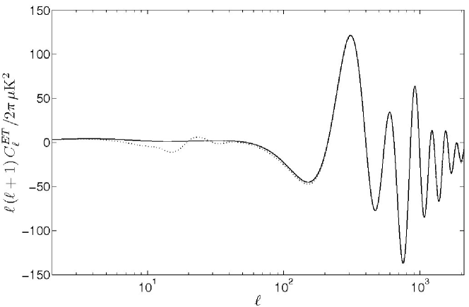
Figure 2: CMB angular power spectra for the ET cross correlation in terms of $\ell$. Solid and dotted lines show the resulting spectra for $D_{1}=0$ and $D_{1}=10^{11}$, respectively.

The $C^{ET}_{\ell}$ spectrum corresponding to $D_{1}=10^{11}$ is represented in the dotted line of Fig. 2. This line slightly deviates with respect to the solid one, which has been obtained for $D_{1}=0$. These small $C^{ET}_{\ell}$ deviations are visible for $\ell$ smaller than $\sim 200$. Nevertheless, for $D_{1}=10^{11}$, the $C^{TT}_{\ell}$ spectrum would be too different from that shown in the solid line of Fig. 1 and, consequently, this high $D_{1}$ value is not admissible. The same occurs with the $C^{EE}_{\ell}$ spectrum, which begins to be different from that of the case $D_{1}=0$ for values as great as $D_{1}\simeq 10^{13}$. All this means that VT–CMBFAST rightly estimates the $C^{ET}_{\ell}$ and $C^{EE}_{\ell}$ coefficients, but they are negligible for any realistic $|D_{1}|$ value smaller than $8\times 10^{8}$ (dotted-dashed line of Fig. 1).

In order to understand some of the above results, it is worthwhile to show some outputs given by VT–CMBFAST. In Fig. 3, these outputs are represented –in terms of the redshift $z$– for appropriate spatial scales. The chosen outputs are the following functions of $z$: $T_{1}=a\ddot{h}+\dot{a}\dot{h}$, $T_{2}=\dot{h}$, and $T_{3}=\dot{\eta}$, which have been chosen by the following reasons: (a) they are involved in the equations describing the evolution of the photon distribution function [see Eq. (63) in mb95 ], which are used to calculate the CMB angular power spectra, and (b) they depend on time derivatives of the metric perturbations $\eta$ and $h$, whose VT and GR values start to be different at some redshift which must be estimated (see I).

Functions $T_{1}$, $T_{2}$, and $T_{3}$ have been obtained for the code runs leading to the solid and dotted-dashed spectra of Fig. 1, which correspond to $D_{1}=0$ (GR) and $D_{1}=8\times 10^{8}$ (VT), respectively. In the top panel of Fig. (3), the spatial scale is $L\simeq 16h^{-1}\ Mpc$ (used to define the standard parameter $\sigma_{8}$). In the top left ($T_{1}$) and top right ($T_{3}$) panels, the blue dashed lines correspond to GR, whereas the red dotted ones show the outputs in VT for the chosen $D_{1}$ value. The dotted lines (VT) oscillate around the dashed ones (GR). In the top central ($T_{2}$) panel, the red dashed lines correspond to VT, whereas the blue dotted ones show the outputs in GR. The dotted line (GR) oscillates around the dashed one (VT). In all cases we find oscillations. Quantities $T_{1}$ and $T_{3}$ oscillate in VT, but not in GR, whereas $T_{2}$ undergoes oscillations in GR, but not in VT. In all the middle panels, the spatial scale is $L\simeq 200h^{-1}\ Mpc$. In these panels the blue dashed lines have been obtained for GR, and the red dotted ones correspond to VT. By comparing the middle panels with the top ones one easily see that, as the spatial scale grows, the functions $T_{1}$ and $T_{2}$ obtained in GR and VT tend to the same limit. For the spatial scale $L\simeq 200h^{-1}\ Mpc$, the dotted and dashed lines of the middle left and central panels are indistinguishable; however, for the same scale, the $T_{3}$ function corresponding to VT oscillates around its GR values (middle right panel). In the bottom panels, the spatial scale is varied to see the behavior of the $T_{3}$ function. The spatial scales increase from left to right taking on the values $L\simeq 700h^{-1}\ Mpc$ (left), $L\simeq 2800h^{-1}\ Mpc$ (central), and $L\simeq 31400h^{-1}\ Mpc$ (right). As it follows from these panels, the oscillations of function $T_{3}$ decrease as the spatial scale increases, which means that the VT and GR values of $T_{3}$ converge as the spatial scale grows. We see that, for scales larger than $\sim 2800h^{-1}\ Mpc$ there are no significant differences between the VT and GR values of $T_{3}$ (see the bottom central and right panels).

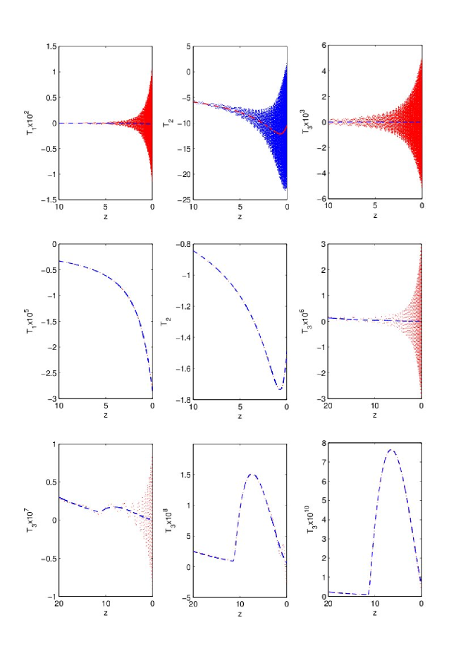
Figure 3: Top and middle panels: representation of functions $T_{1}=a\ddot{h}+\dot{a}\dot{h}$ (left), $T_{2}=\dot{h}$ (central), and $T_{3}=\dot{\eta}$ (right) in terms of the redshift $z$ for various scales of interest. Top (middle) panels correspond to a spatial scale close to $16h^{-1}\ Mpc$ ($200h^{-1}\ Mpc$). Bottom panels: function $T_{3}$ for scales of $700h^{-1}\ Mpc$ (left), $2800h^{-1}\ Mpc$ (central), and $31400h^{-1}\ Mpc$ (right). In all panels the dotted (dashed) lines show the functions of VT (GR), except in the top central panel, where the dotted (dashed) lines correspond to GR (VT).

The oscillatory character of the differences between GR and VT explains the fact that the VT spectra do not depend on the sign of $D_{1}$, but only on $|D_{1}|$. Equivalent oscillations arise for both $D_{1}$ and $-D_{1}$. Moreover, from Fig. 3 it follows that, if there are oscillatory differences for a certain spatial scale, they are visible for redshifts smaller than $\sim 5$. These redshifts are significantly larger than $0.8$, which is very close to the redshift corresponding to the beginning of the accelerated expansion ($2\rho_{v}=\rho_{matter}$) in the standard concordance model. Moreover, there are no visible oscillatory differences for very large spatial scales, which qualitatively explains why the GR and VT angular power spectra of Figs. 1 and 2 are more and more similar as $\ell$ decreases from $\ell\sim 5$.

Figure 1 suggests that VT may explain the observational data for some non vanishing $D_{1}$ values combined with appropriate values of the remaining parameters. In order to verify this suspicion, let us use a set of parameters to fit appropriate observational data and VT predictions by means of statistical techniques. The code VT-COSMOMC has been used to perform this fit. We have used the seven parameters of Table 1. Only data relative to SNe Ia and CMB anisotropy observations have been taken into account. This choice seems to be appropriate, since the same data lead to very good fits in the standard GR model. The CMB angular power spectra used by VT-COSMOMC were obtained from the WMAP7 data. The last version of COSMOMC uses data from PLANCK and WMAP9; nevertheless, this version was delivered very recently, after the numerical calculations presented in this paper –which are good enough– were finished. Further research based on PLANCK spectra will be developed in future (see Sec. 5).

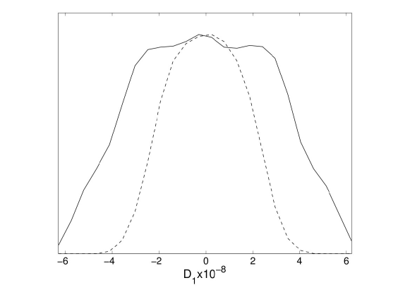
Figure 4: Solid (dashed) line shows the mean (marginalized) likelihood function for the parameter $D_{1}$ of VT.

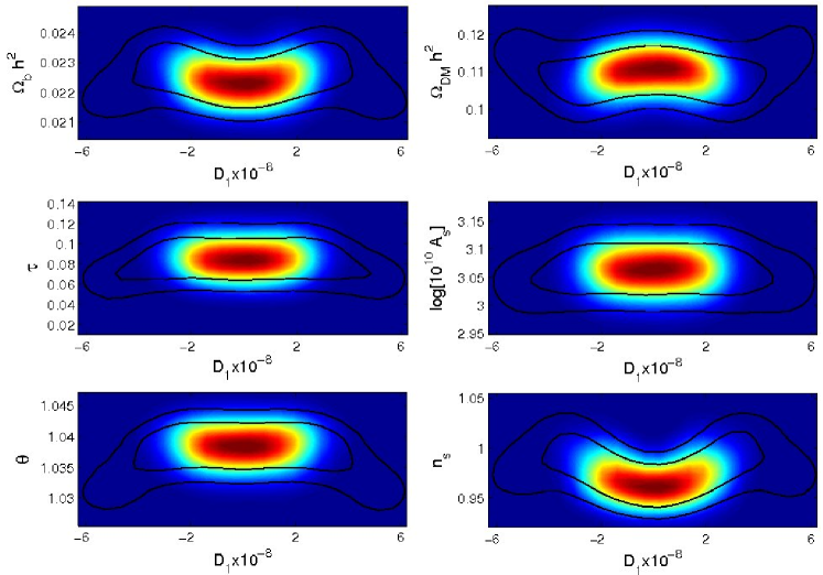
Figure 5: Each panel corresponds to a pair of parameters. In all panels, one of these parameters is $D_{1}$. The second parameter is one of the six GR parameters listed in Table 1. The grayscale (red-yellow-blue) central region of each panel represents the mean likelihood function. The external (internal) contour shows the $2\sigma$ ($1\sigma$) confidence level in the marginalized case.

Results obtained with VT-COSMOMC are presented in Figs. 4 and 5 and also in Table 1. Let us discuss the most significant aspects of these results. The best fit in VT corresponds to the parameters shown in the fourth row of Table 1, where we see that $D_{1}$ is very close to $2\times 10^{7}$ and the remaining parameters take on values very similar to those of the first row (best fit in standard GR cosmology); hence, in a representation as that of Fig. 1, the angular power spectra of the VT and GR best fits would be indistinguishable. From the point of view of the best fits, both theories are equivalent, which is a good result for a theory as VT, which explains the existence of the cosmological constant. Nevertheless, let us now show that a more exhaustive statistical analysis strongly suggests that VT cosmological models may be preferable.

The dashed (solid) line of Fig. 4 shows the marginalized (mean) likelihood function (with arbitrary normalization) for the analyzed samples of parameters. In the marginalized case, the six parameters of the GR models are fixed and their values are taken to be identical to those of the best VT fit. Although the dashed line has a maximum for $D_{1}\simeq 2\times 10^{7}$, this curve is rather flat around the maximum and it may be stated that values of $D_{1}$ satisfying the relation $-10^{8}<D_{1}<10^{8}$ are also very likely in order to explain the observation. A broader interval of admissible $D_{1}$ values is found from the solid line (mean likelihood) of Fig. 4. This line has a wide plateau around the maximum at $D_{1}\simeq 2\times 10^{7}$, which means that, if the seven parameters are varied (no marginalization), the mean likelihood function takes on values similar to the maximum one for the $D_{1}$ values of the plateau and, moreover, for any of these $D_{1}$ values, there must be likelihood values greater than the mean one, which must be closer to the maximum likelihood (see Fig. 4). A visual analysis of this figure shows that the plateau is approximately defined by the condition $-3\times 10^{8}<D_{1}<3\times 10^{8}$. For these values and appropriate values of the six GR parameters, which will be different from those of the best fit, the observations may be explained with high probability.

More statistical information may be found in Fig. 5, where each panel shows the likelihood function for a pair of parameters. One of them is always $D_{1}$ and the second one is another of the parameters of Table 1. The grayscale (red-yellow-blue) central zone shows the mean likelihood of the considered parameter samples. In all cases, the $D_{1}$ values of this zone approximately satisfy the relation $-3\times 10^{8}<D_{1}<3\times 10^{8}$, in agreement with the discussion of the last paragraph. The internal (external) contour shows the 68% (95%) confidence limit in the marginalized case, in which, the remaining five parameters are fixed according to the best VT fit (fourth row of Table 1). The external contour tell us that, inside the seven intervals (one for each parameter) defined by the lower and upper limits given in the two last rows of Table 1, there are values of the seven parameters explaining the observational data at $2\sigma$ confidence. In particular, the $D_{1}$ value will be in the interval ($-5.3\times 10^{8},\,5.3\times 10^{8}$). According to Fig. 1, for $|D_{1}|\leq 3\times 10^{8}$, the VT and GR angular power spectra of the CMB are slightly different for $\ell\leq 250$, and these spectra are rather different for $|D_{1}|\leq 5.3\times 10^{8}$. All these considerations indicate that there are good fits for a wide interval of $|D_{1}|$ values. This fact seems to be related to: (a) the cosmic variance, which is important for the range of $\ell$ values ($\ell<250$) affected by the condition $D_{1}\neq 0$, and (b) the CMB spectrum, which remains unchanged for $\ell>250$ whatever the $D_{1}$ value maybe. We may also verify that, for the remaining six parameters, the VT intervals defined by the lower and upper $2\sigma$ limits given in the two last rows of Table 1 are wider than the corresponding intervals of the GR model ($D_{1}=0$), whose lower and upper $2\sigma$ limits are shown in the second and third rows of the same Table. All these considerations indicate that the seven parameters are coupled and, consequently, parameter $D_{1}$ plays an important role in VT statistical fits.

V Discussion and conclusions

It has been proved (see Sec. II) that, in EE and VT, the background energy density of the field $A^{\mu}$ plays the role of dark energy with $W=-1$; nevertheless, in order to have a positive dark energy, the coupling constant $\gamma$ must be positive (negative) in VT (EE).

In Eqs. (6) and (11), we see that the last terms of the right hand side have the same form but opposite signs. This fact has been justified with a detailed variational study. Since only these terms contribute to $\rho^{A}_{B}$ ($F^{\mu\nu}=0$ in the background), this density appears to have opposite signs in Eqs. (17) and (18), which correspond to EE and VT, respectively. From these equations and the condition $\rho^{A}_{B}>0$, the sign of $\gamma$ is fixed in both theories.

Since the conservation equations (4) have played a very relevant role in the Lagrangian formulation of EE, a few words about the conserved currents of VT and EE are worthwhile. As it follows from Eq. (3), the conserved current of EE is $J_{\mu}+J^{{}^{A}}_{\mu}$ [see Eq. (4)]. In the case $J^{\mu}=0$ (VT), the Lagrangian $-\frac{1}{4}F^{\mu\nu}F_{\mu\nu}+\gamma(\nabla_{\mu}A^{\mu})^{2}$ is invariant under the local gauge transformations $A^{\prime\mu}=A^{\mu}+\nabla^{\mu}\Phi$, with $\nabla_{\mu}\nabla^{\mu}\Phi=0$ and, consequently, the second Noether theorem may be applied to get the conserved current $J^{{}^{A}}_{\mu}$ [see Eq. (12]. For $J^{\mu}\neq 0$ (EE), the Lagrangian is $-\frac{1}{4}F^{\mu\nu}F_{\mu\nu}+\gamma(\nabla_{\mu}A^{\mu})^{2}+J^{\mu}A_{\mu}$. It may be easily proved that this Lagrangian is also gauge invariant, under the above local gauge transformation, if $J^{\mu}$ is replaced by $\nabla^{\nu}F_{\mu\nu}-J^{{}^{A}}_{\mu}$, namely, if $J^{\mu}$ is constrained to satisfy the field equations (3). From the resulting gauge invariant Lagrangian and the second Noether theorem, it follows that the conserved current is $J_{\mu}+J^{{}^{A}}_{\mu}$. In general, currents $J_{\mu}$ and $J^{{}^{A}}_{\mu}$ are not expected to be separately conserved, since we should not have two independent conserved currents associated to an unique group of local gauge transformations.

We have verified that, in a neutral universe where the background current $J^{\mu}$ and its scalar perturbations vanish (dal12, ), EE and VT lead to the same cosmological conclusions in the study of both the background universe and the scalar perturbations; nevertheless, as a result of the negative $\gamma$ value involved in EE, which would lead to problems with quantification, our results are presented in the framework of VT. This theory is based on action (8), which has four terms. Deviations with respect to GR only can be produced by the second and third terms, which vanish for $\gamma=\varepsilon=0$. In other words, for vanishing $\gamma$ and $\varepsilon$, action 8 reduces to the GR one and, consequently, for small enough values of $\gamma$ and $\varepsilon$, VT and GR would be indistinguishable.

According to Eq. (20), parameter $\gamma$ must satisfy the relation $\gamma(\nabla\cdot A)_{B}^{2}=\rho_{v}$. Furthermore, as it has been shown in previous sections (see also paper dal12 ), there are no additional cosmological constraints to be satisfied by the constant quantities $\gamma$ and $(\nabla\cdot A)_{B}$. It is due to the fact that these quantities may be eliminated from the evolution equations of the scalar perturbations. Moreover, these equations do not involve the parameter $\varepsilon$ either. This means that, in cosmology, quantities $\gamma$ and $\varepsilon$ only must satisfy the inequality $2\varepsilon-\gamma>0$.

The strength of gravitation is fixed by the first term of action 8 (proportional to R). The second and third terms –related to gravitation in VT– should involve small coupling constants compatible with the weak character of the gravitational interaction; namely, these constant must be compatible with the fact that the strength of the gravitational field is very low as compared to the strengths of electroweak and strong interactions. Appropriate values of the free constants $\gamma$ and $\varepsilon$ –which have not been fixed by cosmological considerations– may be chosen (with the constraint $2\varepsilon-\gamma>0$) to guaranty that the second and third terms of action 8 have nothing to do with strong and electroweak interactions, but with gravity.

A general formalism to evolve the VT scalar modes from the redshift $z=10^{8}$ is developed. The evolution equations and the initial conditions for all the scalar modes are written in momentum space (Bardeen formalism) by using the synchronous gauge. Moreover, the scalar mode associated to the VT field $A^{\mu}$ is chosen in such a way that: (i) it evolves separately and, (ii) it is involved in the evolution equations for the scalar modes of GR cosmology (standard model). Our methodology is analogous to that used by Ma & Bertschinger mb95 . Equations and initial conditions are fully general.

Our calculations with VT-CMBFAST prove that some time derivatives of the metric modes $\eta$ and $h$ (which are involved in the evolution equations of the CMB photon distribution function) evolve in the same way –in both GR and VT– until redshifts $\sim 10$; then, the evolution of these derivatives starts to be different in both theories and, at redshifts $z\leq 5$, they take on fully different values in VT and GR, except for very large spatial scales (see Sec. IV). Deviations between VT and GR are oscillatory. They explain the differences between the CMB angular power spectra of both theories for $\ell\leq 250$.

By using the code VT-COSMOMC, WMAP7 and SNe Ia data have been adjusted to VT predictions by using seven parameters. In the standard GR model, either WMAP7 or WMAP9 and other data (supernovae, matter power spectrum and so on) are well fitted with a minimal model involving six parameters (see jar11 ; hin12 ). We add the new parameter $D_{1}$ which is characteristic of VT to perform a fit based on seven parameters. In the best fit, the six common parameters of the GR and VT models are very similar, which means that VT works as well as GR; however, there are also good fits for $D_{1}$ values satisfying the condition $|D_{1}|<3\times 10^{8}$ and, moreover, at 95% confidence, the parameter $D_{1}$ satisfies the condition $|D_{1}|<5.3\times 10^{8}$ (see Sec. IV). The fact that we have found good fits for a wide range of $D_{1}$ values strongly suggests that VT models may explain cosmological observations better than GR. It is due to the existence of an additional degree of freedom (parameter $D_{1}$), which has a good behavior and helps us to get good fits.

A new version of COSMOMC has been recently delivered. It includes PLANCK CMB spectra. We are trying to modify this version for future applications to VT. New fits based on the modified code would use better observational data and, moreover, these fits could involve more parameters, lensing, and other effects; nevertheless, the study of these general fits is beyond the paper scope. Here, we essentially point out that VT deserves attention, since it is a theory which explains: the existence of a cosmological constant, and recent CMB and SNe Ia observations (with a minimal model involving seven parameters). Moreover, parameter $D_{1}$ seems to be a help to fit predictions and observations in VT and, consequently, VT fits seem to be more promising than the GR ones.

- (1) J. Beltrán Jiménez and A.L. Maroto, J. Cosmol. Astropart. Phys., 03, 016 (2009)
- (2) J. Beltrán Jiménez, T.S. Koivisto, A.L. Maroto and D.F. Mota, J. Cosmol. Astropart. Phys., 10, 029 (2009)
- (3) J. Beltrán Jiménez and A.L. Maroto, Phys. Rev. D, 83, 023514 (2011)
- (4) R. Dale and D. Sáez, Phys. Rev. D, 85, 124047 (2012)
- (5) J.M. Bardeen, Phys. Rev D, 22, 1882 (1980)
- (6) W. Hu and M. White, Phys. Rev. D, 56, 596 (1997)
- (7) R. Dale, J.A. Morales and D. Sáez, arXiv:0906.2085[astro-ph.CO]
- (8) J. Beltrán Jiménez and A.L. Maroto, J. Cosmol. Astropart. Phys., 02, 025 (2009)
- (9) C.P. Ma and E. Bertschinger, Astrophys. J., 455, 7 (1995)
- (10) U. Seljak and M. Zaldarriaga, Astrophys. J., 469, 437 (1996)
- (11) A. Lewis, A. Challinor and A. Lasenby, Astrophys. J., 538, 473 (2000)
- (12) A. Lewis and S. Bridle, Phys. Rev. D, 66, 103511 (2002)
- (13) S.W. Hawking and G.F.R. Ellis The large scale structure of space-time, Cambridge Monographs on Mathematical Physics (Cambridge University Press, NY, 1999).
- (14) C.M. Will, Theory and experiment in gravitational physics (Cambridge University Press, NY, 1993).
- (15) C.M. Will, Living Rev. Relativity, 9, 3 (2006)
- (16) J.A. Morales and D. Sáez, Phys. Rev. D, 75, 043011 (2007)
- (17) J.A. Morales and D. Sáez, Astrophys. J., 678, 583 (2008)
- (18) N. Jarosik et al, Astrophys. J. Suppl. Ser., 192, 14 (2011)
- (19) G. Hinshaw, et al., Astrophys. J. Suppl. Ser., 208 19 (2013)