Singular diffusion and criticality in a confined sandpile

Abstract

We investigate the behavior of a two-state sandpile model subjected to a confining potential in one and two dimensions. From the microdynamical description of this simple model with its intrinsic exclusion mechanism, it is possible to derive a continuum nonlinear diffusion equation that displays singularities in both the diffusion and drift terms. The stationary-state solutions of this equation, which maximizes the Fermi-Dirac entropy, are in perfect agreement with the spatial profiles of time-averaged occupancy obtained from model numerical simulations in one as well as in two dimensions. Surprisingly, our results also show that, regardless of dimensionality, the presence of a confining potential can lead to the emergence of typical attributes of critical behavior in the two-state sandpile model, namely, a power-law tail in the distribution of avalanche sizes.

Physical processes involving anomalous diffusion are typically associated with systems in which the mean square displacement of their elementary units follows a nonlinear power-law relationship with time, $\sigma^{2}\propto t^{\alpha}$, with an exponent $\alpha\neq 1$, in contrast with linear standard diffusion ($\alpha=1$). Instead of being a rare phenomenon, as suggested by its own denomination, anomalous diffusion, however, appears rather ubiquitously in Nature, playing an important role in a variety of scientific and technological applications, such as fluid flow through disordered porous media Lukyanov2012 , surface growth Spohn1993 , diffusion in fractal-like substrates Stephenson1995 ; Andrade1997 ; Buldyrev2001 ; Costa2003 ; Havlin2002 , turbulent diffusion in the atmosphere Richardson1926 ; Hentschel1984 , spatial spreading of cells Simpson2011 and biological populations Colombo2012 , cellular transport Caspi2002 , and cytoplasmic crowding in cells Weiss2004 . Anomalous diffusion can also manifest its non-Gaussian behavior in terms of nonlinear Fokker-Plank equations Lenzi2001 ; Malacarne2001 ; Malacarne2002 ; DaSilva2004 ; Lenzi2005 , which is the case, for example, of the dynamics of interacting vortices in disordered superconductors Zapperi2001 ; Moreira2002 ; Miguel2003 ; Andrade2010 , diffusion in dusty plasma Liu2008 ; Barrozo2009 , and pedestrian motion Barrozo2009 .

The extreme case of nonlinear behavior in diffusive systems certainly corresponds to singular diffusion. For instance, in some physical conditions, the diffusion of adsorbates on a surface can be strongly nonlinear Ehrlich1980 ; Gomer1990 ; Myshlyavtsev1995 , with a surface diffusion coefficient that depends on the local coverage $\theta$ as, $D\propto{\left|\theta-\theta_{c}\right|^{-\alpha}}$. The study of surface-diffusion mechanisms is crucial for the understanding of technologically important processes related with physical adsorption Vidali1991 and catalytic surface reactions Manandhar2003 ; Hofmann2005 ; Schmidtbauer2012 . In particular, a singularity in the coverage dependence of the diffusion coefficient is frequently associated to continuous phase transitions Myshlyavtsev1995 .

A direct connection between singular diffusion and self-organized criticality Bak1987 has been disclosed by Carlson et al. Carlson1990 ; Carlson1993 in terms of a two-state one-dimensional sandpile model with a driving mechanism, where grains are added at one end of the pile and fall off at the other end. Besides exhibiting a self-organized state, the continuum limit of this simple model leads to a nonlinear diffusion equation, where the diffusion coefficient not only depends on the local density, but also displays a singularity at a “critical” density value Carlson1990 ; Carlson1993 ; Carlson1995 ; Kadanoff1992 ; Barbu2010 . Indeed, the critical aspects of this model remain to be elucidated, specially due to the fact that the most prominent sign of criticality, namely, long-range power-law spatial correlations are not present in the original setup of the simulated dynamical system. Here we show that the addition of a confining potential to the two-state sandpile model solves this problem, namely, power-law tails are observed in the distribution of avalanche sizes in both one- and two-dimensional versions of the theoretical model. Moreover, our results reveal that the continuum description of the model contains singular nonlinearities in both the diffusion and drift terms of the resulting partial differential equation for the transport process.

The microscopic model investigated in this study consists of an one-dimensional lattice of size $N_{s}$ on which $N$ particles ($N_{s}\gg N$) are randomly placed in such a way that the height $h(i)$ of each site $i=1,\,\dots,\,N_{s}$ is either $1$ or $0$. At each step, one grain is chosen randomly to move to the left or to the right with equal probability. If the nearest neighbor in the chosen direction is occupied, the grain jumps instantly to the next-nearest neighbor in the same direction. If this site is also occupied, the particle keeps jumping until it finally reaches an empty site $j$ Carlson1990 . This type of exchange driving mechanism for closed systems has been previously introduced in the context of fluctuations and local equilibrium in self-organizing systems Carlson1993 ; Montakhab1998 . Here, an external confining potential is applied to the system by introducing a non-uniform transition probability from site $i$ to $j$. Precisely, each site is mapped into the continuous interval $[-L/2,L/2]$, and the position $x_{i}=i(L/N_{s})-L/2$ is associated with a potential energy $\phi(x_{i})$. For a given transition, we compute $\Delta\phi_{ij}=\phi(x_{j})-\phi(x_{i})$ and use the following Metropolis rules:

$$\left.\begin{array}[]{c}h(i)\rightarrow h(i)-1\\ h(j)\rightarrow h(j)+1\end{array}\right\} \text{ if }\Delta\phi_{ij}<0\text{ or }r<w=\exp\left(-\beta\Delta\phi_{ij}\right)$$

$$\left.\begin{array}[]{c}h(i)\rightarrow h(i)\\ h(j)\rightarrow h(j)\end{array}\right\} \text{ if }\Delta\phi_{ij}>0\text{ and }r>w,$$

where $r$ is a uniform random number in the interval $[0,1]$, $\beta\equiv 1/k_{B}T$, $T$ is the temperature of the thermal reservoir in contact with the system, $k_{B}$ is the Boltzmann constant, and we count one unit of time for every $N$ grains moved. The effect of decreasing the temperature is equivalent to increasing the strength of the external potential.

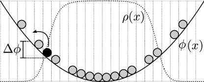
Figure 1: Illustration of the model. A grain moves if $\Delta\phi_{ij}<0$ or $r<e^{-\beta\Delta\phi_{ij}}$, $r\in[0,1]$. As a result, the average density $\rho$ has a maximum in the region where $\phi$ is minimum.

A continuum limit for this microscopic model can be obtained rigorously. If we let $\rho_{i}=\rho(x_{i},\,t)$ be the probability that site $i$ located at $x_{i}$ is occupied at time $t$ and $\phi_{i}=\phi(x_{i})$, a master equation can then be written as,

$$\frac{\partial\rho_{i}}{\partial t}=-\frac{\rho_{i}}{\tau}\left\{\frac{1}{2}\sum_{j=1}^{\infty}(1-\rho_{i+j})\min[1,e^{-\beta(\phi_{i+j}-\phi_{i})}]\prod_{k=1}^{j-1}\rho_{i+k}+\frac{1}{2}\sum_{j=1}^{\infty}(1-\rho_{i-j})\min[1,e^{-\beta(\phi_{i-j}-\phi_{i})}]\prod_{k=1}^{j-1}\rho_{i-k}\right\}\\ +\frac{(1-\rho_{i})}{\tau}\left\{\frac{1}{2}\sum_{j=1}^{\infty}\min[1,e^{-\beta(\phi_{i}-\phi_{i+j})}]\prod_{k=1}^{j}\rho_{i+k}+\frac{1}{2}\sum_{j=1}^{\infty}\min[1,e^{-\beta(\phi_{i}-\phi_{i-j})}]\prod_{k=1}^{j}\rho_{i-k}\right\},$$ (1)

where $\tau$ is the average time between transitions. The first term on the right side is the transition rate corresponding to site $i$ being occupied at time $t$ and loosing the grain, while the second term accounts for the transition rate for an empty site $i$ to gain a grain. Considering that $\tau\approx\delta^{2}/2D$, where $\delta$ is the lattice spacing and $D>0$ is a constant with dimensions of diffusion coefficient ($cm^{2}/s$), and keeping terms to order $\mathcal{O}(\delta^{2})$, it can be shown that, as $\delta$ goes to zero, the following nonlinear diffusion equation holds:

$$\frac{\partial\rho}{\partial t}=D\frac{\partial}{\partial x}\left[\frac{(1+\rho)}{(1-\rho)^{3}}\frac{\partial\rho}{\partial x}+\frac{(1+\rho)}{(1-\rho)^{2}}\beta\frac{d\phi}{dx}\rho\right].$$ (2)

Details of this derivation can be found in the Supplementary Material. Equation (2) can be related to a nonlinear Fokker-Planck equation (FPE) of the form,

$$\frac{\partial\rho}{\partial t}=\frac{\partial}{\partial x}\left[\Omega(\rho)\frac{\partial\rho}{\partial x}\right]-\frac{\partial}{\partial x}\left[A(x)\Psi(\rho)\right],$$ (3)

with $\Omega(\rho)=D(1+\rho)/(1-\rho)^{3}$, $A(x)=-d\phi(x)/dx$, and $\Psi(\rho)=D\beta\rho(1+\rho)/(1-\rho)^{2}$. Considering the FPE (3), with $dF/dt\leq 0,$where $F=U-\gamma S,$ $U=\int dx\rho(x,t)\phi(x)$, and the entropy taken in a general form as $S[\rho]=\int dx\,g[\rho(x)]$, with $g(0)=g(1)=0$ and $d^{2}g/d\rho^{2}\leq 0$, we obtain Schwammle2007 ; Andrade2010 ,

$$-\gamma\frac{d^{2}g(\rho)}{d\rho^{2}}=\frac{\Omega(\rho)}{\Psi(\rho)}=\frac{1}{\beta\rho(1-\rho)},$$ (4)

where $\gamma$ is a positive Lagrange multiplier. This equation has a solution in the form,

$$g(\rho)=\frac{-\rho\ln\rho-(1-\rho)\ln(1-\rho)}{\beta\gamma},$$ (5)

for which the entropy $S[\rho]=\int dx\,g[\rho(x)]$ reduces to the entropy of a Fermi gas, with $\gamma=T$. The functional $\Omega(\rho)$ physically corresponds to a diffusion coefficient which depends on $\rho(x,\,t)$. Clearly it diverges for $\rho=1$ and the diffusion coefficient has the same form as for the case without the external potential Carlson1990 . The functional $\Psi(\rho)$ is related to a drift due to the external potential, and also diverges for $\rho=1$.

The stationary state solution for Eq. (2) can be readily obtained by imposing that $\partial\rho/\partial t=0$, and both $\rho(x)$ and $\partial\rho/\partial x$ go to zero as $x\rightarrow\pm\infty$,

$$\rho_{\text{st}}(x)=\frac{1}{1+e^{\beta[\phi(x)-\mu]}},$$ (6)

where $\mu$ is an integration constant. This solution corresponds to the Fermi-Dirac distribution, with $\mu$ as the chemical potential. It matches exactly the distribution obtained by making the entropy (5) an extreme, where the parameter $\mu$ can be determined by the normalization,

$$\int_{-\infty}^{\infty}\frac{\rho(x,t)}{\delta}dx=N.$$ (7)

As shown in Fig. 2, the solution (6) is in excellent agreement with the spatial profiles of time-averaged occupancy obtained from numerical simulations for distinct forms of the potential, namely, $\phi(x)=\kappa{|x|}^{n}$, $n=1,\,2,\,3$ and $4$, and different values of $\kappa$ (or temperature). As the strength of the confining potential increases (or the temperature decreases), the maximum occupancy density at the center of the potential approaches unity, $\rho_{\text{st}}\approx 1$, and the peak in the profile becomes narrower. At this point, since the density can not increase further, any additional confinement leads to more sites with a maximum average occupancy, resulting in the characteristic step shape of the Fermi-Dirac distribution.

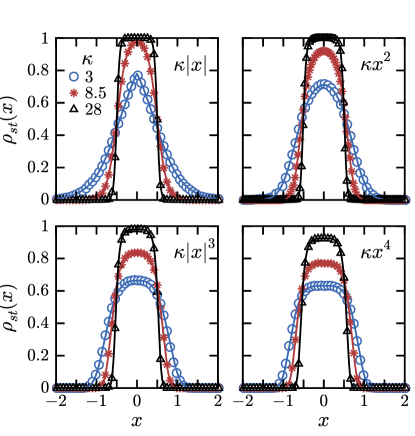
Figure 2: Comparison between numerical and analytical stationary-state solutions for the occupancy density of the confined two-state sandpile model in 1D. Numerical results are for a system with $N=4000$ grains, $\beta=1$, and potentials given by $\phi(x)=\kappa{|x|}^{n}$, with $n=1,\,2,\,3$ and $4$. The $\kappa$ values are $3.0$ (blue circles), $8.5$ (red stars) and $28$ (black triangles). The analytical results are given by the solution (6) with no fitting parameter and shown as solid lines for all values of $\kappa$. In all simulations, we use $\delta=1/N$.

The confining potential substantially changes the way grains hop to the nearest empty site. The average distribution of avalanches with size $s$ is shown in Fig. 3 for the case of parabolic confinement and different values of $\kappa$. Here, a hop from site $i$ to $j$ corresponds to an avalanche of size $|j-i|$. As depicted, the distribution is an exponential decay for small values of $\kappa$, in agreement with the derivation for the two-state sandpile model without confinement Carlson1990 . By increasing $\kappa$ large avalanche become more probable, since the confinement favors the occurrence of large clusters of grains near the center of the potential. For a critical value of $\kappa\approx 28$ the average occupancy near the center of the potential approaches 1, and the avalanche size distribution exhibits a power-law characteristics for a wide range of sizes. More precisely, as indicated in Fig. 3, $\mathcal{P}(s)\sim s^{-\alpha}$, with $\alpha=0.87\pm 0.02$. Further increase in the confinement parameter $\kappa$ eventually leads to the occurrence of a very large cluster, with near all the grains, located at the center of the symmetrical potential, and, as a result, a pronounced peak for $s/N\sim 1$ become evident in the avalanche size distribution. This corresponds to avalanches spanning from one side of the system to the other, passing through the center of the symmetrical potential.

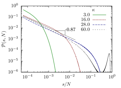
Figure 3: Stationary-state distributions of avalanche sizes $s$ for the confined two-state sandpile model in 1D. The number of grains is $N=16000$ and $\beta=1$ for the numerical simulations. For $\kappa\approx 28$ the distribution displays power-law behavior, $P(s)\sim s^{-\alpha}$, followed by a cutoff of the form $\exp(-s^{2})$ at the order of the system size. The least-squares fit to the data of a power-law in the scaling region gives $\alpha=0.87\pm 0.02$.

Next we extend our results to two-dimensional systems. In this case, a grain at position $\mathbf{r}_{i}=(x_{i},y_{i})$ moves in a randomly selected direction until it finds the nearest empty site. The transition is then accepted or not following the same Metropolis algorithm previously described for the 1D case, but now with a confining parabolic potential of the form, $\phi(\mathbf{r}_{i})=\kappa(x_{i}^{2}+y_{i}^{2})$. Figure 4 shows the radial profile of the time average occupancy in 2D, $\rho(r)$, obtained from numerical simulations for different values of the strength of the confining potential $\kappa$. The qualitative behavior of the system is the same as in 1D, namely, the stronger the confining potential, the narrower the profile with the maximum occupancy at the center of the potential approaching unit. Further increasing $\kappa$, the occupancy saturates at $\rho\sim 1$ and the profile becomes broader, resembling a step function. Also shown in Fig. 4 are typical snapshots of the grain positions for the same values of $\kappa$, colored according to the size of the clusters they belong to. If the confinement is weak, all sizes of clusters are present, with larger clusters located at the center of the potential. As $\kappa$ increases, larger and more compact clusters are favored at the center of the potential, tending to a limit where most of the grains belong to a single, compact cluster with an irregular surface.

As for the one-dimensional case, the results in Fig. 4 computed for distinct confinement strengths show that the average radial profiles of occupancy in 2D are perfectly consistent with the Fermi-Dirac distribution,

$$\rho_{\text{st}}(r)=\frac{1}{1+e^{\beta[\phi(r)-\mu]}},$$ (8)

but now subjected to the normalization condition,

$$\int_{0}^{2\pi}\int_{0}^{\infty}\frac{\rho(r,t)}{\delta^{2}}rdrd\phi=N\quad\Rightarrow\quad\mu=\frac{1}{\beta}\ln\left(e^{\beta\frac{N\delta^{2}\kappa}{\pi}}-1\right).$$ (9)

This excellent agreement between simulations and the Fermi-Dirac distribution suggests that in two-dimensions the system satisfies the generalization of the FPE (3) to higher dimensions, which is of the form,

$$\frac{\partial\rho}{\partial t}=\nabla\cdot\left[\Omega(\rho)\nabla\rho\right]-\nabla\cdot\left[\mathbf{A}(\mathbf{r})\Psi_{(}\rho)\right],$$ (10)

where $\mathbf{A}(r)=-\nabla\phi(\mathbf{r})$, with the condition (4) still valid in 2D.

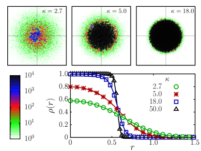
Figure 4: On the top are snapshots of the grain positions for different values of $\kappa$ at the stationary state. Different colors correspond to distinct clusters and the color code in the bar indicates the cluster size, which increases from white to black. On the bottom are the stationary-state profiles of the average occupancy, $\rho(r)$, for two-state two-dimensional sandpiles confined by a parabolic potential. The system size is $N=100000$ and different curves correspond to distinct values of the potential strength $\kappa$. The solid lines correspond to the analytical solutions (8) without fitting parameters, calculated for different values of $\kappa$ and $\beta=1$. In all simulations, we use $\delta=1/\sqrt{N}$.

Figure 5 depicts the avalanche size distribution for the two-dimensional system. Here $s$ corresponds to the number of sites visited in the fixed chosen direction until an empty site is found and the transition is accepted. As shown in Fig. 5, the avalanche size distribution changes from an exponential decay for $\kappa=2.7$ to a distribution with a well defined peak near the size of the system for $\kappa=50.0$. In 2D a characteristic size for the avalanches is the diameter of the system $D\approx 2\sqrt{N/\pi}$. Our numerical results show that, for a critical value of the confining parameter, $\kappa\approx 18$, the presence of the confining potential leads to an avalanche size distribution that obeys a power law for small avalanche sizes, $P(s)\sim s^{-\alpha}$, with an exponent $\alpha=1.09\pm 0.04$.

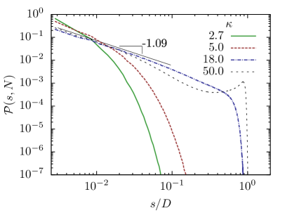
Figure 5: Stationary-state distributions of avalanche sizes $s$ for the confined two-state sandpile model in 2D. The number of grains is $N=100000$ and $\beta=1$ for the numerical simulations. For $\kappa\approx 18$ the distribution displays power-law behavior, $P(s)\sim s^{-\alpha}$, followed by a cutoff of the form $\exp(-s^{2})$ at the order of the characteristic system size, $D\approx 2\sqrt{N/\pi}$. The least-squares fit to the data of a power-law in the scaling region gives $\alpha=1.09\pm 0.04$.

In summary, here we studied the effect of a confining potential on the behavior of a two-state sandpile model in one and two dimensions. A continuum nonlinear diffusion equation could be derived from the microdynamical description of the model that is shown to be perfectly consistent with the transport of grains observed from numerical simulations. This equation, besides displaying singularities in both the diffusion and drift terms, has a stationary-state solution for the spatial profiles of average occupancy of grains that maximizes the Fermi-Dirac entropy. Moreover, our results show that the introduction of a confining potential to the two-state sandpile model, if properly tuned, can lead to power-law behavior in the distribution of grain-jump sizes. These results are rather surprising since 1D systems usually do not display non-trivial critical states nor power-law behavior. They can be explained in terms of the non-homogeneity introduced by the confining potential and the complex fluctuations due to the singular-diffusion dynamics. The extension to two-dimensions reveals that the strongly nonlinear features of the system together with the intrinsic exclusion mechanism present in the model also lead to the Fermi-Dirac distribution for the occupancy profiles. Power-law distributions of avalanches sizes are also observed in 2D at critical values of the intensity of the confining potential.

We thank the Brazilian agencies CNPq, CAPES, and FUNCAP for financial support.

References

- (1) A. V. Lukyanov, M. M. Sushchikh, M. J. Baines, and T. G. Theofanous, Phys. Rev. Lett. 109, 214501 (2012).
- (2) H. Spohn, J. Phys. I 3, 69 (1993).
- (3) J. Stephenson, Physica A 222, 234 (1995).
- (4) J. S. Andrade Jr., D. A. Street, Y. Shibusa, S. Havlin, and H. E. Stanley, Phys. Rev. E 55, 772 (1997).
- (5) S. V. Buldyrev, S. Havlin, A. Ya. Kazakov, M. G. E. da Luz, E. P. Raposo, H. E. Stanley, and G. M. Viswanathan, Phys. Rev. E 64, 041108 (2001).
- (6) M. H. A. S. Costa, A. D. Araujo, H. F. da Silva, and J. S. Andrade Jr., Phys. Rev. E 67, 061406 (2003).
- (7) S. Havlin and D. Ben-Avraham, Advan. Phys 51, 187 (2002).
- (8) L. F. Richardson, Proc. R. Soc. London, Ser. A 110, 709 (1926).
- (9) H. G. E. Hentschel and I. Procaccia, Phys. Rev. A 29, 1461 (1984).
- (10) M. J. Simpson, R. E. Baker, and S. W. McCue, Phys. Rev. E 83, 021901 (2011).
- (11) E. H. Colombo and C. Anteneodo, Phys. Rev. E 86, 036215 (2012).
- (12) A. Caspi, R. Granek, and M. Elbaum, Phys. Rev. E 66, 011916 (2002).
- (13) M. Weiss, M. Elsner, F. Kartberg, and T. Nilsson, Biophys. J. 87, 3518 (2004).
- (14) E. K. Lenzi, C. Anteneodo, and L. Borland, Phys. Rev. E 63, 051109 (2001).
- (15) L. C. Malacarne, R. S. Mendes, I. T. Pedron, and E. K. Lenzi, Phys. Rev. E 63, 030101 (2001).
- (16) L. C. Malacarne, R. S. Mendes, I. T. Pedron, and E. K. Lenzi, Phys. Rev. E 65, 052101 (2002).
- (17) P. C. da Silva, L. R. da Silva, E. K. Lenzi, R. S. Mendes, and L. C. Malacarne, Physica A 342, 16 (2004).
- (18) E. K. Lenzi, R. S. Mendes, J. S. Andrade Jr., L. R. da Silva, and L. S. Lucena, Phys. Rev. E 71, 052101 (2005).
- (19) S. Zapperi, A. A. Moreira, and J. S. Andrade Jr., Phys. Rev. Lett. 86, 3622 (2001).
- (20) A. A. Moreira, J. S. Andrade Jr., J. Mendes Filho, and S. Zapperi, Phys. Rev. B 66, 174507 (2002).
- (21) M. Miguel, J. S. Andrade Jr., and S. Zapperi, Braz. J. Phys. 33, 557 (2003).
- (22) J. S. Andrade Jr., G. F. T. da Silva, A. A. Moreira, F. D. Nobre, and E. M. F. Curado, Phys. Rev. Lett. 105, 260601 (2010).
- (23) B. Liu and J. Goree, Phys. Rev. Lett. 100, 055003 (2008).
- (24) P. Barrozo, A. A. Moreira, J. A. Aguiar and J. S. Andrade Jr., Phys. Rev. B 80, 104513 (2009).
- (25) G. Ehrlich and K. Stolt, Ann. Rev. Phys. Chem. 31, 603 (1980).
- (26) R. Gomer, Rep. Prog. Phys. 53, 917 (1990).
- (27) A. V. Myshlyavtsev, A. A. Stepanov, C. Uebing, and V. P. Zhdanov, Phys. Rev. B 52, 5977 (1995).
- (28) G. Vidali, G. Ihm, H-Y. Kim, and M. W. Cole, Surf. Sci. Rep. 12, 135 (1991).
- (29) P. Manandhar, J. Jang, G. C. Schatz, M. A. Ratner, and S. Hong, Phys. Rev. Lett. 90, 115505 (2003).
- (30) S. Hofmann, G. Csányi, A. C. Ferrari, M. C. Payne, and J. Robertson, Phys. Rev. Lett. 95, 036101 (2005).
- (31) J. Schmidtbauer, R. Bansen, R. Heimburger T. Teubner, T. Boeck, and R. Fornari, Appl. Phys. Lett. 101, 043105 (2012).
- (32) P. Bak, C. Tang and K. Wiesenfeld, Phys. Rev. Lett. 59, 381 (1987).
- (33) J. M. Carlson, J. T. Chayes, E. R. Grannan, and G. H. Swindle, Phys. Rev. Lett. 65, 2547 (1990).
- (34) J. M. Carlson, E. R. Grannan, C. Singh, and G. H. Swindle, Phys. Rev. E 48, 688 (1993).
- (35) J. M. Carlson and G. H. Swindle, Proc. Natl. Acad. Sci. USA 92, 6712 (1995).
- (36) L. P. Kadanoff, A. B. Chhabra, A. J. Kolan, M. J. Feigenbaum, and I. Procaccia, Phys. Rev. A 45, 6095 (1992).
- (37) V. Barbu, Annu. Rev. Control 34, 52 (2010).
- (38) A. Montakhab and J. M. Carlson, Phys. Rev. E 58, 5608 (1998).
- (39) V. Schwämmle, F. D. Nobre, and E. M. F. Curado, Phys. Rev. E 76, 041123 (2007).