Detecting a Corrupted Area
in a 2-Dimensional Space

Abstract

Motivated by the fact that 2-dimensional data have become popularly used in many applications without being much considered its integrity checking. We introduce the problem of detecting a corrupted area in a 2-dimensional space, and investigate two possible efficient approaches and show their time and space complexities. Also, we briefly introduce the idea of an approximation scheme using a hash sieve and suggest a novel “adaptive tree” structure revealing granularity of information.

Keywords: Detect Corrupted Area, Signed Hashes, Integrity

1 Introduction

In recent years, with the help of the development of fast and inexpensive computers, many emerging applications have adopted 2-dimensional data such as image or GIS as well as 1-dimensional data to provide various and advanced services to customers. However, such 2-dimensional data can be partially changed or modified (maliciously or accidentally).

In 2007, “Mayo Clinic and IBM have created a collaborative research facility aimed at advancing medical imaging technologies to improve the quality of patient care by providing quicker critical diagnosis, such as the growth or shrinkage of tumors [1]”. There are a few related work such as authentication and recovery image by using a digital watermarking method [5]. However, their models are quite different from our model.

The main difference is that they actually modify an original data by adding watermarking information to the original data to detect the modification of image, and they do not guarantee the detection of tampering of data by allowing a small changes of bits of image without being detected. Since they do not use (signed) hash values, they do not require to store additional data structure for detecting data modification.

Moreover, [5] only consider pure image data rather than general 2-dimensional data (e.g., GIS as well as images). Motivated by this, we investigate the problem of efficiently finding a corrupted region in a given 2-dimensional space.

The rest of the paper is organized as follows. We present models and assumptions in Section 2. Then we investigate two approaches in Section 3, and Section 4. We also briefly introduce other possible approaches in Section 6, and conclude in Section 7.

2 Models and Assumptions

Given a 2-dimensional space $N=m\times m$, we want to find a corrupted area $C$ which is composed of $t$ number of times of $c$ where $c$ is the smallest unit (e.g., a pixel). Suppose Alice has the original data of space $N$. Bob has an actual data of space $N$ which might be corrupted, and he wants to detect a corrupted area $C$ if $N$ is corrupted

We assume that a corrupted area is a single connected shape. Since there is no prior information in a given 2-dimensional area, we do not know whether the area was corrupted or not, and do not know the size or shape of the corrupted area. Also, we assume that all data in a given region are uniformly distributed. That means that all data have the same level of importance to be scanned and thus have the same granularity of importance.

The heart of the problem is finding one corrupted cell, because once we know such a cell we can “spread out” from that cell to the remaining corrupted one in breadth-first like fashion and in time $O(C)$. This is why we focus in this section on the problem of finding one corrupted cell.

We consider two models in this paper. Suppose Alice’s original data and Bob’s actual data are stored in a same computer. Then two sets of data can be compared directly without storing any additional data structure using a probabilistic method and we will describe it in Section 3. Note that this model requires an assumption that Alice’s original data have not been altered, and should be kept in a safe storage.

However, it is hard to achieve such safe devices in our general computing environment. Computers and their storages are vulnerable to many types of malicious behaviors such as malware infection, computer bug, or hacking. In addition, if Alice’s original data and Bob’s actual data are stored in different machines, then direct comparison is not appropriate.

Thus, in this model we use signed hash values, assuming that Bob already downloaded these signed hash values and its verification key from a server or ISP. Note that the signature key is not stored. We will describe this second model in Section 4. Note that a server could be trusted signing server or untrusted distributor of signed hash values proposed in our previous paper [3].

3 Finding a Corrupted Cell Using a Probabilistic Method

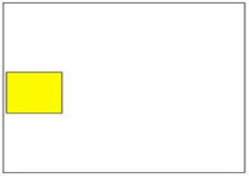
(a) A small yellow rectangle is a corrupted area

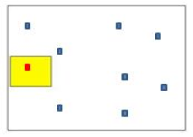
(b) Tiny blue rectangles are randomly chosen cells in each step until find a tiny red corrupted cell in a corrupted area

Figure 1: Probabilistic Method

Let the random variable $X$ be the number of trials needed to obtain a success to find $c$, and let $P\{X=k\}$ be the probability of success to find $c$ (Fig. 1). If $k\leq N-C$ then $P\{X=k\}=\bigl{(}1-\frac{C}{N}\bigr{)}\bigl{(}1-\frac{C}{N-1}\bigr{)}\bigl{(}1-\frac{C}{N-2}\bigr{)}\cdots\bigl{(}1-\frac{C}{N-(k-2)}\bigr{)}\bigl{(}\frac{C}{N-(k-1)}\bigr{)}$. Note that if $k>N-C$ then $P\{X=k\}=1$. Let $E[X]$ be the expected number of trials to find $c$ at $k^{th}$ trial. Then

$$E[X] = \sum_{k=1}^{N}kP\{X=k\}$$

$$= \biggl{(}1-\frac{C}{N}\biggr{)}+2\biggl{(}1-\frac{C}{N-1}\biggr{)}+\cdots+(k-1)\biggl{(}{1-\frac{C}{N-(k-2)}}\biggr{)}+k\biggl{(}\frac{C}{N-(k-1)}\biggr{)}$$

If we assume that $C\ll N$ then $\frac{C}{N}\approx\frac{C}{N-1}\approx\cdots\approx\frac{C}{N-(k-1)}$ is $p$ where $p=\frac{C}{N}$, and $N-C$ is approximate to $N$. Then we have an approximation of $E[X]$ as follows :

$$E[X]=\sum_{k=1}^{\infty}k(1-p)^{k-1}p=\frac{1}{p}=\frac{N}{C}$$

Thus the time to find $c$ is $\frac{N}{C}$. Once we find $c$, we can find $C$ by spreading up to $4t$. Therefore, the total time to find a corrupted area $C$ is $O(\frac{N}{C}+t)$. Note that this scheme does not require to store any additional data structure to find a corrupted area $C$.

4 Detecting a Corrupted Cell Using Signed Hashes

We consider two cases – one in which the time is measured by the number of cells whose hashes are computed, and the other in which time is measured by the number of signature verifications. The latter is motivated by the fact that a signature verification is much more time consuming than a cryptographic hash computation.

4.1 Minimizing Signature Verifications

In this model we store a number $s(N)$ of signatures for some subsets of the $m\times m$ cells, hence $s(N)$ is the space complexity of the scheme. The signature key is not locally stored to protect against compromise of the local machine (that would compromise the signature key). In the search for a corrupted cell, a basic comparison operation consists of checking whether the signature for a subset of the $N$ cells matches the current values at those cells; such a comparison costs 1 in the model considered here (even though the comparison involves looking at all the cells of the subset, it counts as 1 because there is only 1 signature verification that it does).

4.2 A preliminary Scheme

We store a signed hash for each of the four $(m/2)\times(m/2)$ quadrants, and recursively so on for each quadrant (Fig. 2).

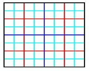
(a) Recursive Quadrants

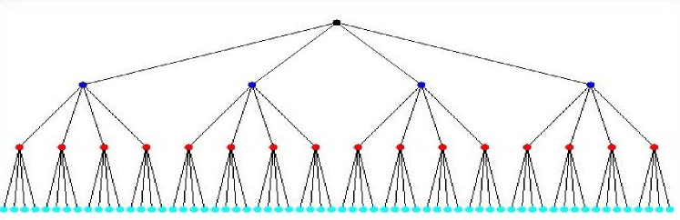
(b) Signed Hash Values Corresponding Recursive Quadrants

Figure 2: Preliminary Method

Thus the space complexity obeys the recurrence

$$s(N)=4+4S(N/4)$$

$$S(1)=1$$

This implies $S(N)\leq c_{1}N-c_{2}$, where $c_{1},c_{2}$ are constant and it can be proved by induction as follows. The basis of the induction is $N=1$, in which case we do have $1\leq c_{1}*1-c_{2}$ as long as we choose $c_{1}\geq 1+c_{2}$. For the inductive step, we assume the claim holds for values smaller than $N$ and we show that it must then hold for $N$. Using the induction hypothesis in the recurrence equation gives:

$$s(N)=4+4S(N/4)\leq 4+4(c_{1}N/4)-4c_{2}=4+c_{1}N-4c_{2}$$

which is $\leq c_{1}N-c_{2}$ as long as we choose $c_{2}$ such that $4-3c_{2}\leq 0$, i.e., $c_{2}\geq 4/3$.

This structure allows searching for a corrupted cell in logarithmic time, as follows: Check if each of the 4 quadrants matches the corresponding stored signature, and if not recurse on one of the quadrants that does not match its stored signature (if more than one does not match then recurse on any one that does not match).

The number $T(N)$ of signature verifications done obeys the recurrence

$$T(N)\leq 4+T(N/4)$$

$$T(1)=1$$

and therefore $T(N)$ is $O(\log N)$.

4.3 An Improved Scheme

The following scheme can substantially outperform it if $C$ is large.

We first show that, in a 1-dimensional version of the problem (i.e., an array of $N$ entries of which $C$ are corrupted), we can find a corrupted cell in a binary search fashion by doing $t=\log(N/C)$ signature verifications. This is done as follows: First we test the left half of the array, then the right half, and if both are corrupted then we have already found a corrupted cell (the middle cell) otherwise we recurse in one of the two halves (the corrupted one). After $i$ such iterations the search region has shrunk down to the size of $N/2^{i}$, and success at finding a corrupted cell must occur prior to reaching a situation where $N/2^{i}>C$, which is equivalent to saying that $i<\log(N/C)$.

To use a 1-dimensional approach as part of a solution of a 2-dimensional problem, we need to assume that the $C$ damaged cells form a region that is not only connected but also convex in the sense that for any row or column the subset of corrupted cells on that row or column forms a connected 1-dimensional region.

The above 1-dimensional solution suggests the following approach to the 2-dimensional problem: Modify the 2-dimensional preliminary scheme given in the previous subsection so that it operates in a manner similar to the preliminary scheme except that we would switch to (one or two) 1-dimensional problem(s) as soon as we reach a situation where more than one quadrant is found to be corrupted:

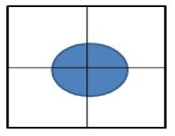
(a) “$+$” Boundary

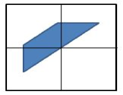
(b) “T” Boundary

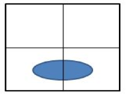
(c) “I” Boundary

Figure 3: Improved Scheme

We would then switch to the union of the boundaries between all pairs if corrupted quadrants. This union could be shaped like a cross (“$+$”), a “T”, an “I”, a “–” , etc (Fig. 3). The continuation of the search would be on the (one or two) one-dimensional regions that make up that union. Specifically, if $C^{\prime}$ of the cells of the resulting 1-dimensional problems are corrupted, then we would complete the job in a number of signature verifications that is $O(\log(\sqrt{N}/C^{\prime}))$. The number of signature verifications done prior to switching to this 1-dimensional mode is $\leq\log(N/C)$ because after $i$ such verifications the size of the square region being searched has become $N/2^{i}$ and we will have surely switched to 1-dimensional mode before we end up with $N/2^{i}<C$.

Of course the above requires storing signatures for the “boundary” one-dimensional problems in addition to the 4 signatures for the quadrants. There are at most two such one-dimensional problems, of size $m=\sqrt{N}$ each. Because the number of signatures for a one-dimensional problem of size $\sqrt{N}$ is $2\sqrt{N}-1$, the space complexity now obeys the recurrence

$$s(N)=4+2(2\sqrt{N}-1)+4S(N/4)=2+4\sqrt{N}+4S(N/4)$$

$$S(1)=1$$

We show now that the above implies $S(N)\leq c_{1}N-c_{2}\sqrt{N}$, where $c_{1},c_{2}$ are constant (in other words the space is still $O(N)$, no worse than in the preliminary scheme). The proof, by induction on $N$, is as follows. The basis of the induction is $N=1$, in which case we do have $1\leq c_{1}-c_{2}$ as long as we choose $c_{1}\geq 1+c_{2}$. For the inductive step, we assume the claim holds for values smaller than $N$ and we show that it must then hold for $N$. Using the induction hypothesis in the recurrence equation gives:

$$s(N)=2+4\sqrt{N}+4S(N/4)\leq 2+4\sqrt{N}+4(c_{1}N/4)-4c_{2}\sqrt{N/4}=2+c_{1}N-2c_{2}\sqrt{N}$$

which is $\leq c_{1}N-c_{2}\sqrt{N}$ as long as $2-c_{2}\sqrt{N}\leq 0$, i.e., $c_{2}\geq 2/\sqrt{N}$, which is true as long as we choose $c_{2}\geq 2$.

4.4 Analysis of Preliminary Scheme

This section briefly analyzes the scheme of the previous section.

The preliminary scheme’s time recurrence is

$$T(N)=N+T(N/4)$$

$$T(1)=1$$

The solution becomes $T(N)=O(N)$.

The time recurrence of the 1-dimensional scheme is

$$T(N)=N+T(N/2)$$

if $N\geq 2C$, and

$$T(N)=N$$

if $N<2C$. The solution is

$$T(N)=N+(N/2)+(N/2^{2})+\cdots+(N/2^{i})$$

where $i$ is the smallest integer for which $N/2^{i}<2C$. Using the above equation twice in $T(N)=2T(N)-T(N)$ gives:

$$T(N)=2T(N)-T(N)=2(N+(N/2)+(N/2^{2})+\cdots+(N/2^{i}))-(N+(N/2)+(N/2^{2})+\cdots+(N/2^{i}))$$

which gives $T(N)=2N-(N/2^{i})$. Since the definition of $i$ implies that $C<N/2^{i}$, we finally get

$$T(N)=2N-(N/2^{i})<2N-C$$

.

The 2-dimensional solution which converted to the 1-dimensional can be similarly analyzed and its $T(N)$ becomes

$$T(N)<2N-C+O(\sqrt{N})$$

where the lower order term of $\sqrt{N}$ comes from the 1-dimensional part of the scheme.

The next section provides and analyzes a scheme that is specifically deigned for the “number of cells touched” cost model.

5 Minimizing Cells Accessed Using A Sifting Approach

We now count the cost of verifying the signature for a region $R$ to be proportional to the size of that region. That is, it is the number of cells in $R$ (whereas in the previous model we counted it as 1).

We first give a 1-dimensional version of the approach. For the convenience we assume $N$ and $C$ are powers of 2. For $k=1,2,3,\ldots$ we do the following Stage $k$ until we identify a corrupted cell:

• Stage $k$ consists of checking the integrity of each cell whose position is a multiple of $N/2^{k}$ and that was not already tested in any of the earlier stages $1,2,\ldots,k-1$.

The number of stages is at most $i$ where $i$ is the integer for which $N/2^{i}=C$, i.e., i = $\log(N/C)$. The work done at stage 1 is 2 (the cells at positions $N/2$ and $N$), the work done at stage 2 is 2 (the cells at positions $N/4$ and $3N/4$), at stage 3 it is 4, etc. In general, for $k\geq 2$, the work needs to be done at stage $k$ is $2^{k}-2^{k-1}=2^{k-1}$. The total work is therefore

$$2+\sum_{k=2}^{i}2^{k-1}=O(2^{i})$$

which is $O(N/C)$. Note that this is much better than the $O(N-C)$ achieved by using the 1-dimensional scheme of the previous section.

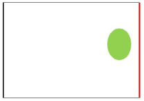
(a) Stage $k$=1

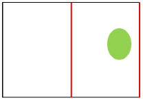
(b) Stage $k$=2

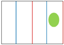
(c) Stage $k$=3

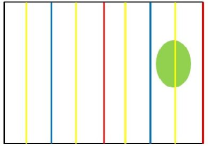
(d) A corrupted oval green area is detected at stage $k$=4

Figure 4: A Sifting Approach

The scheme extends to 2 dimensions by using it on the columns and then, once a column with corrupted cells has been found, using the above 1-dimensional on that column. The process of identifying a corrupted column is as follows (Fig. 4). For $k=1,2,3,\ldots$ we do the following Stage $k$ until we have identified a corrupted cell:

• Stage $k$ consists of checking the integrity of each column whose number is a multiple of $N/2^{k}$ and that was not already tested in any of the earlier stages $1,2,\ldots,k-1$.

The number of stages is at most $i$ where $i$ is the integer for which $N/2^{i}=C$, i.e., i = $\log(N/C)$. The work done at stage 1 is $2\sqrt{N}$ (the columns numbered $N/2$ and $N$), the work done at stage 2 is $2\sqrt{N}$ (the columns at positions $N/4$ and $3N/4$), at stage 3 it is $4\sqrt{N}$, etc. In general, for $k\geq 2$, the work done at stage $k$ is

$$(2^{k}-2^{k-1})\sqrt{N}=2^{k-1}\sqrt{N}$$

The total work is therefore

$$(2+\sum_{k=2}^{i}2^{k-1})\sqrt{N}=O(2^{i}\sqrt{N})$$

which is $O(N^{1.5}/C)$. Once a column with corrupted cells is identified, we can find a corrupted cell within that column in time $O(\sqrt{N})$, so the dominant cost is the $O(N^{1.5}/C)$ for finding the column.

5.1 Hybrid Approach

Let $A_{1}$ be the improved scheme and $A_{2}$ be the sift scheme. It is clear that if $C<\sqrt{N}$, $A_{1}$ is better and $A_{2}$ is better otherwise. However, we do not know the value of $C$ in advance since we assume that only information we are given is a 2-dimensional area. We do not know whether it is corrupted or not. Neither do we know the size of corrupted area.

However, we can perform the previous one “in parallel” by alternating between $A_{1}$ and $A_{2}$. We stop as soon as one of them succeeds. We do this because we do not know the value of $C$ in advance. Thus we cannot choose which of the two is better for that unknown $C$. The overall complexity of this hybrid solution for the 2-dimensional case becomes:

$$T(N)=O(N*\min\{1,\sqrt{N}/C\})$$

6 Other Approaches

In the following sections, we briefly introduce two different approaches by relaxing assumptions that we used in previous sections. One is an approximation scheme, and the other is an adaptive tree structure.

6.1 Approximation Scheme

First, we give an idea of an approximation scheme by reducing the number of signed hash values using a sparse spacing filling curve (e.g, Hilbert curve or Z-curve) [2, 4]. The key idea is that we store two layers of hash values: horizontal and vertical hash layers, and each layer consists of $O(\sqrt{N})$ number of hash values of horizontal and vertical layer respectively such that a sparse space fillings curve of signed hashes will be displayed when those two layers are overlapped. In this case, the time to find a corrupted cell $T(N)$ will be $O(\sqrt{N})$, and the size of stored hash values $s(N)$ as well which are much better.

Since the overlapped layers form a sieve so that we can sieve a corrupted area, we can find an approximate corrupted area $C^{\prime}$ (instead of a precise shape of corrupted area $C$ without spreading after we found a corrupted cell), and this might help to detect multiple corrupted areas.

However, one of issues in this model is the level of sparseness of a space filling curve. Even though a space filling curve reduces a dimension by one, it is quite dense. Thus we want to use a sparse version, but it is not easy to measure how much we should make it sparse since it is closely related with the size of corrupted area which is not a given information in advance.

6.2 Adaptive Tree

In this section, we consider the case when data do not have the same level of importance. For example, an image of internal organs of human body probably has different probabilities of having tumors; The probability of having tumors in layers of fat or water will be negligible unlike lung or stomach. In this model, we can assign different levels of granularity of importance in a region.

Motivated by this, we introduce a novel tree structure, “adaptive tree”, for signed hash values which includes granularity information. We create a tree such that the number of children of each node at $h$ is $2^{h}$ where $h$ is a height of a tree. The degree of a node is $2^{h}$ at depth 0 (i.e. root) and $2^{t-1}$ at depth 1 and then $2^{1}$ at depth $h-1$. Thus

$$2^{h}2^{h-1}2^{h-2}\cdots 2^{1}=N$$

and $h\approx\sqrt{2\lceil(logN+1)\rceil}$ (Fig. 5).

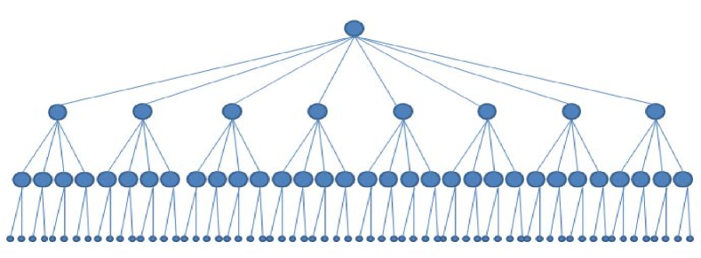
Figure 5: Adaptive Tree (e.g.,$N=64$)

Thus the height of a tree $h$ is $O(\sqrt{logN})$. Note that the size of each child becomes $N/(2^{\sqrt{logN}})$. This adaptive tree structure has a shorter height, and it gives you the more detail information (i.e., smaller granularity), the more you go down the tree.

7 Conclusion

We introduced the problem of detecting a corrupted area in a 2-dimensional space, and investigated some possible solutions under the two different models efficiently, and analyzed their time and space complexities. Our approaches do not tolerate even 1-bit modification of original data unlike watermarking schemes [5]. We also briefly described approximate scheme with much better time and space complexity by relaxing assumptions. Furthermore, we introduce a novel “adaptive tree” structure revealing granularity of information. We will provide a full extended version of this paper in a very near future.

References

- [1] Mayo clinic and ibm establish medical imaging research center. Available at http://www-03.ibm.com/press/us/en/presskit/23251.wss.
- [2] J. K. Lawder and P. J. H. King. Using space-filling curves for multi-dimensional indexing. In Advances in Database, 17th British National Conference on Database, July 2000.
- [3] Y. C. M. Atallah and A. Kundu. Efficient data authentication in an environment of untrusted third-party distributions. In In Proceedings of the 24th International Conference on Data Engineering (ICDE’08), Cancun, Mexico, Apr. 2008.
- [4] J. A. Orenstein and F. A. Manola. Probe spatial data modeling and query processing in an image database application. In IEEE Transaction on Software Engineering, May 1998.
- [5] J. M. Zain and A. N. Muhamad. Authentication watermarking with tamper detection and recovery (aw-tdr). In Proceedings of the International Conference on Electrical Engineering and Informatics, pages 11–20, Institute Teknologi Bandung, Indonesia, June 2007.