Models as Approximations I: Consequences Illustrated with Linear Regression

Abstract

In the early 1980s Halbert White inaugurated a “model-robust” form of statistical inference based on the “sandwich estimator” of standard error. This estimator is known to be “heteroskedasticity-consistent”, but it is less well-known to be “nonlinearity-consistent” as well. Nonlinearity, however, raises fundamental issues because in its presence regressors are not ancillary, hence can’t be treated as fixed. The consequences are deep: (1) population slopes need to be re-interpreted as statistical functionals obtained from OLS fits to largely arbitrary joint ${x\textrm{-}y}$ distributions; (2) the meaning of slope parameters needs to be rethought; (3) the regressor distribution affects the slope parameters; (4) randomness of the regressors becomes a source of sampling variability in slope estimates; (5) inference needs to be based on model-robust standard errors, including sandwich estimators or the ${x\textrm{-}y}$ bootstrap. In theory, model-robust and model-trusting standard errors can deviate by arbitrary magnitudes either way. In practice, significant deviations between them can be detected with a diagnostic test.

1 Introduction

Halbert White’s basic sandwich estimator of standard error for OLS can be described as follows: In a linear model with regressor matrix ${\mathbb{X}}_{\!N\!\times\!(p\!+\!1)}$ and response vector ${\boldsymbol{y}}_{N\!\times\!1}$, start with the familiar derivation of the covariance matrix of the OLS coefficient estimate ${\boldsymbol{\hat{\beta}}}$, but allow heteroskedasticity, ${\boldsymbol{V}}[{\boldsymbol{y}}|{\mathbb{X}}]\!=\!{\boldsymbol{D}}$ diagonal:

$${\boldsymbol{V}}[\,{\boldsymbol{\hat{\beta}}}\,|{\mathbb{X}}]={\boldsymbol{V}}[({\mathbb{X}}{{}^{\prime}\,}\!{\mathbb{X}})^{-1}{\mathbb{X}}{{}^{\prime}\,}{\boldsymbol{y}}\,|{\mathbb{X}}]=({\mathbb{X}}{{}^{\prime}\,}\!{\mathbb{X}})^{-1}({\mathbb{X}}{{}^{\prime}\,}{\boldsymbol{D}}{\mathbb{X}})({\mathbb{X}}{{}^{\prime}\,}\!{\mathbb{X}})^{-1}.$$ (1)

The right hand side has the characteristic “sandwich” form, $({\mathbb{X}}{{}^{\prime}\,}\!{\mathbb{X}})^{-1}$ forming the “bread” and ${\mathbb{X}}{{}^{\prime}\,}{\boldsymbol{D}}{\mathbb{X}}$ the “meat.” Although this sandwich formula does not look actionable for standard error estimation because the variances ${\boldsymbol{D}}_{ii}\!=\!{\sigma}_{i}^{2}$ are not known, White showed that (1) can be estimated asymptotically correctly. If one estimates ${\sigma}_{i}^{2}$ by squared residuals $r_{i}^{2}$, each $r_{i}^{2}$ is not a good estimate, but the averaging implicit in the “meat” provides an asymptotically valid estimate:

$$\boldsymbol{\hat{V}}_{{\!\!\!s\!\!\>a\!\!\>n\!\!\>d}}[\,{\boldsymbol{\hat{\beta}}}\,]~{}~{}{\overset{\Delta}{=}}~{}~{}({\mathbb{X}}{{}^{\prime}\,}\!{\mathbb{X}})^{-1}({\mathbb{X}}{{}^{\prime}\,}{\hat{\boldsymbol{D}}}{\mathbb{X}})({\mathbb{X}}{{}^{\prime}\,}\!{\mathbb{X}})^{-1},$$ (2)

where ${\hat{\boldsymbol{D}}}$ is diagonal with ${\hat{\boldsymbol{D}}}_{ii}\!=\!r_{i}^{2}$. Standard error estimates are obtained by ${\boldsymbol{\hat{{S\!E}}}}_{{{\!\!\>s\!\!\>a\!\!\>n\!\!\>d}}}[\,{\hat{\beta}_{j}}\,]\!=\!\boldsymbol{\hat{V}}_{{\!\!\!s\!\!\>a\!\!\>n\!\!\>d}}[\,{\boldsymbol{\hat{\beta}}}\,]_{jj}^{1/2}$. They are asymptotically valid even if the responses are heteroskedastic, hence the term “Heteroskedasticity-Consistent Covariance Matrix Estimator” in the title of one of White’s (1980b) famous articles.

Lesser known is the following deeper result in one of White’s (1980a, p. 162-3) less widely read articles: the sandwich estimator of standard error is asymptotically correct even in the presence of nonlinearity:

$${\boldsymbol{E}}[\,{\boldsymbol{y}}\,|{\mathbb{X}}]~{}\neq~{}{\mathbb{X}}{\boldsymbol{\beta}}~{}~{}~{}~{}{\rm for~{}all}~{}{\boldsymbol{\beta}}.$$ (3)

The term “heteroskedasticity-consistent” is an unfortunate choice as it obscures the fact that the same estimator of standard error is also “nonlinearity-consistent” when the regressors are treated as random. The sandwich estimator of standard error is therefore “model-robust” not only against second order model violations but first order violations as well. Because of the relative obscurity of this important fact we will pay considerable attention to its implications. In particular we will show how nonlinearity “conspires” with randomness of the regressors

• to make slopes dependent on the regressor distribution and

• to generate sampling variability, even in the absence of noise in the response.

For an intuitive grasp of these effects, the reader may peruse Figure 2 for effect (1) and Figure 4 for effect (2).

From the sandwich estimator (2), the usual model-trusting estimator is obtained by collapsing the sandwich form using homoskedasticity, ${\hat{\boldsymbol{D}}}={\hat{\sigma}}{\boldsymbol{I}}$:

$$\boldsymbol{\hat{V}}_{{\!\!\!lin}}[\,{\boldsymbol{\hat{\beta}}}\,]~{}~{}{\overset{\Delta}{=}}~{}~{}({\mathbb{X}}{{}^{\prime}\,}\!{\mathbb{X}})^{-1}{\hat{\sigma}}^{2},~{}~{}~{}~{}{\hat{\sigma}}^{2}=\|{\boldsymbol{r}}\|^{2}/(N\!\!-\!p\!-\!1).$$

This yields finite-sample unbiased squared standard error estimators ${\boldsymbol{\hat{{S\!E}}}}_{{{\!\!\>l\!\!\;i\!\!\;n}}}^{2}[\,{\hat{\beta}_{j}}\,]\!=\!\boldsymbol{\hat{V}}_{{\!\!\!lin}}[\,{\boldsymbol{\hat{\beta}}}\,]_{jj}$ if the model is first and second order correct: ${\boldsymbol{E}}[{\boldsymbol{y}}\,|{\mathbb{X}}]\!=\!{\mathbb{X}}{\boldsymbol{\beta}}$ (linearity) and ${\boldsymbol{V}}[{\boldsymbol{y}}\,|{\mathbb{X}}]\!=\!\sigma^{2}{\boldsymbol{I}}_{N}$ (homoskedasticity). Assuming distributional correctness (Gaussian errors), one obtains finite-sample correct tests and confidence intervals.

The corresponding tests and confidence intervals based on the sandwich estimator have only an asymptotic justification, but their asymptotic validity holds under much weaker assumptions. In fact, it may rely on no more than the assumption that the rows $(y_{i},{\vec{\boldsymbol{x}}}_{i}^{\prime})$ of the data matrix $({\boldsymbol{y}},{\mathbb{X}})$ are iid samples from a joint multivariate distribution subject to some technical conditions. Thus sandwich-based theory provides asymptotically correct inference that is model-robust. The question then arises what model-robust inference is about: When no model is assumed, what are the parameters, and what is their meaning?

Discussing these questions is a first goal of this article. An established answer is that parameters can be re-interpreted as statistical functionals ${\boldsymbol{\beta}({\boldsymbol{P}})}$ defined on a large nonparametric class of joint distributions ${\boldsymbol{P}}={\boldsymbol{P}}(dy,d{\vec{\boldsymbol{x}}})$ through best approximation (Section 3), sometimes called “projection.” The sandwich estimator produces then asymptotically correct standard errors for the slope functionals ${\beta_{j}}({\boldsymbol{P}})$ (Section 5). Vexing is the question of the meaning of slopes in the presence of nonlinearity as the standard interpretations no longer apply. We will propose interpretations that draw on the notions of case-wise and pairwise slopes after linear adjustment (Section 10).

A second goal of this article is to discuss why the regressors should be treated as random. Based on an ancillarity argument, model-trusting theories tend to condition on the regressors and hence treat them as fixed (Cox and Hinkley 1974, p. 32f, Lehmann and Romano 2008, p. 395ff). However, it will be shown that under misspecification ancillarity of the regressors is violated (Section 4). Here are some implications:

• Population parameters ${\boldsymbol{\beta}}({\boldsymbol{P}})$, now interpreted as statistical functionals, depend on the distribution of the regressors. Thus it matters where the regressors fall. The reason is intuitive: When models are approximations, it matters where the approximation is made; see Figure 2.

• A natural intuition fails, caused by misleading terminology: Nonlinearity — sometimes called “model bias” — does not primarily cause bias in estimates ${\boldsymbol{\beta}}({\boldsymbol{\hat{P}}})$. It causes sampling variability of order $N^{-1/2}$, thereby rivaling error/noise as a source of sampling variability (Section 6).

• A second intuition fails: While it is correct that an inference guarantee conditional on the regressors implies a marginal inference guarantee, this principle is inapplicable because the premise is false — under misspecification there is no inference guarantee conditional on the regressors. The reason is that inference theories that treat regressors as fixed are incapable of correctly accounting for misspecification.

All three implications hold in great generality, but in this article they will be worked out for OLS linear regression to achieve the greatest degree of lucidity.

A third goal of this article is to argue in favor of the “${x\textrm{-}y}$ bootstrap” which resamples observations $({\vec{\boldsymbol{x}}}_{i}^{\prime},y_{i})$. The better known “residual bootstrap” resamples residuals $r_{i}$ and thereby assumes a linear response surface and exchangeable errors. There exists theory to justify both (Freedman (1981) and Mammen (1993), for example), but only the ${x\textrm{-}y}$ bootstrap is model-robust and solves the same problem as the sandwich estimator. In Part II (Buja et al. 2018), it will be shown that the sandwich estimator is a limiting case of the ${x\textrm{-}y}$ bootstrap.

A fourth goal of this article is to practically (Section 2) and theoretically (Section 11) compare model-robust and model-trusting estimators of standard error in the case of OLS linear regression. To this end we define a ratio of asymptotic variances — “${\boldsymbol{R\!A\!V}}$” for short — that describes the discrepancies between the two standard errors in the asymptotic limit.

A fifth goal is to estimate the ${\boldsymbol{R\!A\!V}}$ for use as a test statistic. We derive an asymptotic null distribution to test for model deviations that invalidate the usual standard error of a specific coefficient. The resulting “misspecification test” differs from other such tests in that it answers the question of discrepancies among standard errors directly and separately for each coefficient (Section 12).

A final goal is to briefly discuss issues with sandwich estimators (Section 13): They can be inefficient when models are correctly specified. We additionally point out that they are non-robust to heavy tails in the joint ${x\textrm{-}y}$ distribution. To make sense of this observation, the following distinctions are needed: (1) classical robustness to heavy tails is distinct from model robustness to first and second order model misspecifications; (2) at issue is not robustness (in either sense) of parameter estimates but of standard errors. It is the latter we examine here.

Throughout we use precise notation for clarity, yet this article is not very technical. Many results are elementary, not new, and stated without regularity conditions. Readers may browse the tables and figures and read associated sections that seem most germane. Important notations are shown in boxes.

The present article is limited to OLS linear regression, both for populations and for data. The case permits explicit calculations and lucid interpretations. Part II (Buja et al. 2018) will treat arbitrary regressions at the cost of reduced lucidity. It will also propose new types of diagnostics.

The idea that models are approximations and hence generally “misspecified” to a degree has a long history, most famously expressed by Box (1979). We prefer to quote Cox (1995): “it does not seem helpful just to say that all models are wrong. The very word model implies simplification and idealization.” The history of inference under misspecification can be traced to Cox (1961, 1962), Eicker (1963), Berk(1966, 1970), Huber (1967), before being systematically elaborated by White’s articles (1980a, 1980b, 1981, 1982, among others), capped by a monograph (White 1994). A wide-ranging discussion by Wasserman (2011) calls for “Low Assumptions, High Dimensions.” A book by Davies (2014) elaborates the idea of adequate models for a given sample size. We, the present authors, got involved with this topic through our work on post-selection inference (Berk et al. 2013) because the results of model selection should certainly not be assumed to be “correct.” We compared the obviously model-robust standard errors of the ${x\textrm{-}y}$ bootstrap with the usual ones of linear models theory and found the discrepancies illustrated in Section 2. Attempting to account for these discrepancies became the starting point of the present article.

2 Discrepancies between Standard Errors Illustrated

Table 1 shows regression results for a dataset consisting of a sample of 505 census tracts in Los Angeles that has been used to relate the local number of homeless ($Y$) to covariates for demographics and building usage (Berk et al. 2008). We do not intend a careful modeling exercise but show the raw results of linear regression to illustrate the degree to which discrepancies can arise among three types of standard errors: ${\boldsymbol{S\!E}}_{{\!\!\>l\!\!\;i\!\!\;n}}$ from linear models theory, ${\boldsymbol{S\!E}}_{{\!\!\>b\!\!\;o\!\!\;o\!\!\;t}}$ from the ${x\textrm{-}y}$ bootstrap ($N_{{\!\!\>b\!\!\;o\!\!\;o\!\!\;t}}=100,000$) and ${\boldsymbol{S\!E}}_{{\!\!\>s\!\!\>a\!\!\>n\!\!\>d}}$ from the sandwich estimator (according to MacKinnon and White’s (1985) HC2 proposal). Ratios of standard errors that are far from +1 are shown in bold font.

	${\hat{\beta}_{j}}$	${\boldsymbol{S\!E}}_{{\!\!\>l\!\!\;i\!\!\;n}}$	${\boldsymbol{S\!E}}_{{\!\!\>b\!\!\;o\!\!\;o\!\!\;t}}$	${\boldsymbol{S\!E}}_{{\!\!\>s\!\!\>a\!\!\>n\!\!\>d}}$	$\frac{{\boldsymbol{S\!E}}_{{\!\!\>b\!\!\;o\!\!\;o\!\!\;t}}}{{\boldsymbol{S\!E}}_{{\!\!\>l\!\!\;i\!\!\;n}}}$	$\frac{{\boldsymbol{S\!E}}_{{\!\!\>s\!\!\>a\!\!\>n\!\!\>d}}}{{\boldsymbol{S\!E}}_{{\!\!\>l\!\!\;i\!\!\;n}}}$	$\frac{{\boldsymbol{S\!E}}_{{\!\!\>s\!\!\>a\!\!\>n\!\!\>d}}}{{\boldsymbol{S\!E}}_{{\!\!\>b\!\!\;o\!\!\;o\!\!\;t}}}$	$t_{{\!\!\>l\!\!\;i\!\!\;n}}$	$t_{{\!\!\>b\!\!\;o\!\!\;o\!\!\;t}}$	$t_{{\!\!\>s\!\!\>a\!\!\>n\!\!\>d}}$
Intercept	0.760	22.767	16.505	16.209	0.726	0.712	0.981	0.033	0.046	0.047
MedianIncome ($K)	-0.183	0.187	0.114	0.108	0.610	0.576	0.944	-0.977	-1.601	-1.696
PercVacant	4.629	0.901	1.385	1.363	1.531	1.513	0.988	5.140	3.341	3.396
PercMinority	0.123	0.176	0.165	0.164	0.937	0.932	0.995	0.701	0.748	0.752
PercResidential	-0.050	0.171	0.112	0.111	0.653	0.646	0.988	-0.292	-0.446	-0.453
PercCommercial	0.737	0.273	0.390	0.397	1.438	1.454	1.011	2.700	1.892	1.857
PercIndustrial	0.905	0.321	0.577	0.592	1.801	1.843	1.023	2.818	1.570	1.529

Table 1: LA Homeless Data: Comparison of Standard Errors. See also Table 6 in the Appendix for the Boston Housing Data.

The ratios ${\boldsymbol{S\!E}}_{{\!\!\>s\!\!\>a\!\!\>n\!\!\>d}}/{\boldsymbol{S\!E}}_{{\!\!\>b\!\!\;o\!\!\;o\!\!\;t}}$ show that the sandwich and bootstrap estimators are in good agreement. Not so for the linear models estimates: we have ${\boldsymbol{S\!E}}_{{\!\!\>b\!\!\;o\!\!\;o\!\!\;t}},{\boldsymbol{S\!E}}_{{\!\!\>s\!\!\>a\!\!\>n\!\!\>d}}>{\boldsymbol{S\!E}}_{{\!\!\>l\!\!\;i\!\!\;n}}$ for the regressors PercVacant, PercCommercial and PercIndustrial, and ${\boldsymbol{S\!E}}_{{\!\!\>b\!\!\;o\!\!\;o\!\!\;t}},{\boldsymbol{S\!E}}_{{\!\!\>s\!\!\>a\!\!\>n\!\!\>d}}<{\boldsymbol{S\!E}}_{{\!\!\>l\!\!\;i\!\!\;n}}$ for Intercept, MedianIncome ($K), PercResidential. Only for PercMinority is ${\boldsymbol{S\!E}}_{{\!\!\>l\!\!\;i\!\!\;n}}$ off by less than 10% from ${\boldsymbol{S\!E}}_{{\!\!\>b\!\!\;o\!\!\;o\!\!\;t}}$ and ${\boldsymbol{S\!E}}_{{\!\!\>s\!\!\>a\!\!\>n\!\!\>d}}$. The discrepancies affect outcomes of some of the $t$-tests: Under linear models theory the regressors PercCommercial and PercIndustrial have sizable $t$-values of $2.700$ and $2.818$, respectively, which are reduced to unconvincing values below $1.9$ and $1.6$, respectively, if the ${x\textrm{-}y}$ bootstrap or the sandwich estimator are used. On the other hand, for MedianIncome ($K) the $t$-value $-0.977$ from linear models theory becomes borderline significant with the bootstrap or sandwich estimator if the plausible one-sided alternative with negative sign is used.

A similar exercise with fewer discrepancies but similar conclusions is shown in Appendix B for the Boston Housing data.

Conclusions: (1) ${\boldsymbol{S\!E}}_{{\!\!\>b\!\!\;o\!\!\;o\!\!\;t}}$ and ${\boldsymbol{S\!E}}_{{\!\!\>s\!\!\>a\!\!\>n\!\!\>d}}$ are in substantial agreement; (2) ${\boldsymbol{S\!E}}_{{\!\!\>l\!\!\;i\!\!\;n}}$ on the one hand and $\{{\boldsymbol{S\!E}}_{{\!\!\>b\!\!\;o\!\!\;o\!\!\;t}},{\boldsymbol{S\!E}}_{{\!\!\>s\!\!\>a\!\!\>n\!\!\>d}}\}$ on the other hand can have substantial discrepancies; (3) the discrepancies are specific to regressors.

3 The Population Framework for Linear OLS

As noted earlier, model-robust inference needs a target of estimation that is well-defined outside the linear working model. To this end we need notation for data distributions that are free of model assumptions, essentially relying on iid sampling of ${x\textrm{-}y}$ tuples. Subsequently OLS parameters can be introduced as statistical functionals of these distributions through best linear approximation. This is sometimes called “projection”, meaning that the assumption-free data distribution is “projected” to the “nearest” distribution in the working model.

3.1 Populations for OLS Linear Regression

In an assumption-lean, model-robust population framework for OLS linear regression with random regressors, the ingredients are regressor random variables $X_{1}$, …, $X_{p}$ and a response random variable $Y$. For now the only assumption is that they are all numeric and have a joint distribution, written as

$${\boldsymbol{P}}~{}=~{}{\boldsymbol{P}}({\mathrm{d}}y,{\mathrm{d}}x_{1},...,{\mathrm{d}}x_{p}).$$

Data will consist of iid multivariate samples from this joint distribution (Section 5). No working model for ${\boldsymbol{P}}$ will be assumed.

It is convenient to add a fixed regressor 1 to accommodate an intercept parameter; we may hence write

$${\vec{\boldsymbol{X}}}~{}=~{}(1,X_{1},...,X_{p}){{}^{\prime}\,}$$

for the column random vector of the regressor variables, and ${\vec{\boldsymbol{x}}}=(1,x_{1},...,x_{p}){{}^{\prime}\,}$ for its values. We further write

$${\boldsymbol{P}_{\!\!Y,{\vec{\boldsymbol{X}}}}}={\boldsymbol{P}},~{}~{}~{}~{}{\boldsymbol{P}_{\!\!Y|{\vec{\boldsymbol{X}}}}},~{}~{}~{}~{}{\boldsymbol{P}_{\!\!{\vec{\boldsymbol{X}}}}},$$

for, respectively, the joint distribution of $(Y,{\vec{\boldsymbol{X}}})$, the conditional distribution of $Y$ given ${\vec{\boldsymbol{X}}}$, and the marginal distribution of ${\vec{\boldsymbol{X}}}$. These denote actual data distributions, free of assumptions of a working model.

All variables will be assumed to be square integrable. Required is also that ${\boldsymbol{E}}[{\vec{\boldsymbol{X}}}{\vec{\boldsymbol{X}}}{{}^{\prime}\,}]$ is full-rank, but permitted are nonlinear degeneracies among regressors as when they are functions of underlying independent variables such as in polynomial or B-spline regression or product interactions.

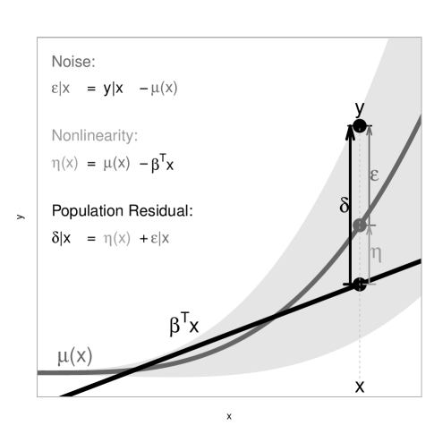
Figure 1: Illustration of the decomposition (5) for linear OLS.

3.2 Targets of Estimation: The OLS Statistical Functional

We write any function $f(X_{1},...,X_{p})$ of the regressors as $f({\vec{\boldsymbol{X}}})$. We will need notation for the “true response surface” $\mu({\vec{\boldsymbol{X}}})$, which is the conditional expectation of $Y$ given ${\vec{\boldsymbol{X}}}$ and the best $L_{2}({\boldsymbol{P}})$ approximation to $Y$ among functions of ${\vec{\boldsymbol{X}}}$. It is not assumed to be linear in ${\vec{\boldsymbol{X}}}$:

$$\mu({\vec{\boldsymbol{X}}})~{}{\overset{\Delta}{=}}~{}{\boldsymbol{E}}[\,Y\,|\,{\vec{\boldsymbol{X}}}\,]~{}=~{}\mathrm{argmin}_{f({\vec{\boldsymbol{X}}})\in L_{2}({\boldsymbol{P}})}\,{\boldsymbol{E}}[(Y-f({\vec{\boldsymbol{X}}}))^{2}]\,.$$

The main definition concerns the best population linear approximation to $Y$, which is the linear function ${{l}}({\vec{\boldsymbol{X}}})={\boldsymbol{\beta}}{{}^{\prime}\,}{\vec{\boldsymbol{X}}}$ with coefficients ${\boldsymbol{\beta}}={\boldsymbol{\beta}({\boldsymbol{P}})}$ given by

$$\begin{array}[]{|lclcl|}\hline\cr~{}~{}~{}~{}{\boldsymbol{\beta}({\boldsymbol{P}}){}}&{\overset{\Delta}{=}}&\mathrm{argmin}_{{\boldsymbol{\beta}}\in{\mathrm{I}\!\mathrm{R}}^{p+1}}\,{\boldsymbol{E}}[(Y\!-\!{\boldsymbol{\beta}}{{}^{\prime}\,}{\vec{\boldsymbol{X}}})^{2}]{}{}{}{}{}&=&{\boldsymbol{E}}[{\vec{\boldsymbol{X}}}{\vec{\boldsymbol{X}}}{{}^{\prime}\,}]^{-1}{\boldsymbol{E}}[{\vec{\boldsymbol{X}}}Y\,]\\ &=&\mathrm{argmin}_{{\boldsymbol{\beta}}\in{\mathrm{I}\!\mathrm{R}}^{p+1}}\,{\boldsymbol{E}}[(\mu({\vec{\boldsymbol{X}}})\!-\!{\boldsymbol{\beta}}{{}^{\prime}\,}{\vec{\boldsymbol{X}}})^{2}]&=&{\boldsymbol{E}}[{\vec{\boldsymbol{X}}}{\vec{\boldsymbol{X}}}{{}^{\prime}\,}]^{-1}{\boldsymbol{E}}[{\vec{\boldsymbol{X}}}\mu({\vec{\boldsymbol{X}}})\,].{}{}{}{}\\ \hline\cr\end{array}$$

Both right hand expressions follow from the population normal equations:

$${\boldsymbol{E}}[{\vec{\boldsymbol{X}}}{\vec{\boldsymbol{X}}}{{}^{\prime}\,}]\,{\boldsymbol{\beta}}-{\boldsymbol{E}}[{\vec{\boldsymbol{X}}}Y]~{}=~{}{\boldsymbol{E}}[{\vec{\boldsymbol{X}}}{\vec{\boldsymbol{X}}}{{}^{\prime}\,}]\,{\boldsymbol{\beta}}-{\boldsymbol{E}}[{\vec{\boldsymbol{X}}}\mu({\vec{\boldsymbol{X}}})]~{}=~{}{\boldsymbol{0}}.$$ (4)

The population coefficients ${\boldsymbol{\beta}({\boldsymbol{P}})}=(\beta_{0}({\boldsymbol{P}}),\beta_{1}({\boldsymbol{P}}),...,\beta_{p}({\boldsymbol{P}})){{}^{\prime}\,}$ form a vector statistical functional, ${\boldsymbol{P}}\mapsto{\boldsymbol{\beta}({\boldsymbol{P}})}$, defined for a large class of joint data distributions ${\boldsymbol{P}}\!=\!{\boldsymbol{P}_{\!\!Y,{\vec{\boldsymbol{X}}}}}$. If the response surface under ${\boldsymbol{P}}$ happens to be linear, $\mu({\vec{\boldsymbol{X}}})\!=\!\tilde{{\boldsymbol{\beta}}}{{}^{\prime}\,}{\vec{\boldsymbol{X}}}$, as it is for example under a Gaussian linear model, $Y|{\vec{\boldsymbol{X}}}\sim{\cal N}(\tilde{{\boldsymbol{\beta}}}{{}^{\prime}\,}{\vec{\boldsymbol{X}}},\sigma^{2})$, then ${\boldsymbol{\beta}({\boldsymbol{P}})}\!=\!\tilde{{\boldsymbol{\beta}}}$. The statistical functional is therefore a natural extension of the traditional meaning of a model parameter, justifying the notation ${\boldsymbol{\beta}}\!=\!{\boldsymbol{\beta}({\boldsymbol{P}})}$. The point is, however, that ${{\boldsymbol{\beta}}(\cdot)}$ is defined even when linearity does not hold. (Depending on the context, we may write ${\boldsymbol{\beta}}$ to mean ${\boldsymbol{\beta}}({\boldsymbol{P}})$.)

3.3 The Noise-Nonlinearity Decomposition for Population OLS

The response $Y$ has the following canonical decompositions:

$$\begin{array}[]{ccccc}Y&=&{\boldsymbol{\beta}}{{}^{\prime}\,}{\vec{\boldsymbol{X}}}&+&\underbrace{(\mu({\vec{\boldsymbol{X}}})-{\boldsymbol{\beta}}{{}^{\prime}\,}{\vec{\boldsymbol{X}}})}~{}+~{}\underbrace{(Y-\mu({\vec{\boldsymbol{X}}}))}\\[10.00002pt] &=&{\boldsymbol{\beta}}{{}^{\prime}\,}{\vec{\boldsymbol{X}}}&+&\underbrace{{\eta}({\vec{\boldsymbol{X}}})~{}~{}~{}~{}~{}~{}+~{}~{}~{}~{}~{}~{}~{}~{}{\epsilon}}\\[10.00002pt] &=&{\boldsymbol{\beta}}{{}^{\prime}\,}{\vec{\boldsymbol{X}}}&+&{\delta}\\ \end{array}$$ (5)

We call ${\epsilon}={\epsilon}|{\vec{\boldsymbol{X}}}$ the noise and ${\eta}={\eta}({\vec{\boldsymbol{X}}})$ the nonlinearity , while for ${\delta}$ there is no standard term, so “population residual” may suffice; see Table 2 and Figure 1. Important to note is that (5) is a decomposition, not a model assumption. In a model-robust framework there is no notion of “error term” in the usual sense; its place is taken by the population residual ${\delta}$ which satisfies few of the usual assumptions made in generative models. It naturally decomposes into a systematic component, the nonlinearity ${\eta}={\eta}({\vec{\boldsymbol{X}}})$, and a random component, the noise ${\epsilon}={\epsilon}|{\vec{\boldsymbol{X}}}$. Model-trusting linear modeling, before conditioning on ${\vec{\boldsymbol{X}}}$, must assume ${\eta}({\vec{\boldsymbol{X}}})\overset{{\boldsymbol{P}}}{=}0$ and ${\epsilon}$ to have the same ${\vec{\boldsymbol{X}}}$-conditional distribution in all of regressor space, that is, to be independent of ${\vec{\boldsymbol{X}}}$. No such assumptions are made here. What is left are orthogonalities satisfied by ${\eta}$ and ${\epsilon}$ in relation to ${\vec{\boldsymbol{X}}}$. If we call independence “strong-sense orthogonality”, we have instead

$$\begin{array}[]{ll}\textrm{weak-sense orthogonality:}~{}~{}~{}~{}~{}{\eta}\perp{\vec{\boldsymbol{X}}}&\!\!({\boldsymbol{E}}[{\eta}\!\cdot\!\!X_{j}]=0~{}~{}\forall j\!=\!0,1,...,p),\\[3.00003pt] \textrm{medium-sense orthogonality:}~{}{\epsilon}\perp L_{2}({\boldsymbol{P}_{\!\!{\vec{\boldsymbol{X}}}}})&\!\!({\boldsymbol{E}}[{\epsilon}\!\cdot\!\!f(\!{\vec{\boldsymbol{X}}}\!)]=0~{}\forall f\!\in\!L_{2}({\boldsymbol{P}_{\!\!{\vec{\boldsymbol{X}}}}})).\end{array}$$ (6)

These are not assumptions but consequences of population OLS and the definitions. Because of the inclusion of an intercept ($j\!=\!0$ and $f\!=\!1$, respectively), both the nonlinearity and noise are marginally centered: ${\boldsymbol{E}}[\,{\eta}\,]={\boldsymbol{E}}[\,{\epsilon}\,]=0$. Importantly, it also follows that ${\epsilon}\perp{\eta}({\vec{\boldsymbol{X}}})$ because ${\eta}$ is just some $f\!\in\!L_{2}({\boldsymbol{P}_{\!\!{\vec{\boldsymbol{X}}}}})$.

In what follows we will need the following natural definitions:

• Conditional noise variance: The noise ${\epsilon}$, not assumed homoskedastic, can have arbitrary conditional distributions ${\boldsymbol{P}}(d{\epsilon}|{\vec{\boldsymbol{X}}}\!=\!{\vec{\boldsymbol{x}}})$ for different ${\vec{\boldsymbol{x}}}$ except for conditional centering and finite conditional variances. Define:

  $${\sigma}^{2}({\vec{\boldsymbol{X}}})~{}~{}{\overset{\Delta}{=}}~{}~{}{\boldsymbol{V}}[\,{\epsilon}\,|{\vec{\boldsymbol{X}}}]~{}=~{}{\boldsymbol{E}}[\,{\epsilon}^{2}\,|\,{\vec{\boldsymbol{X}}}]~{}\overset{{\boldsymbol{P}}}{<}~{}\infty.$$ (7)

  When we use the abbreviation ${\sigma}^{2}$ we will mean ${\sigma}^{2}={\sigma}^{2}({\vec{\boldsymbol{X}}})$ as we will never assume homoskedasticity.

• Conditional mean squared error: This is the conditional MSE of $Y$ w.r.t. the population linear approximation ${\boldsymbol{\beta}}{{}^{\prime}\,}{\vec{\boldsymbol{X}}}$. Its definition and bias-variance decomposition are:

  $${m}^{2}({\vec{\boldsymbol{X}}})~{}~{}{\overset{\Delta}{=}}~{}~{}{\boldsymbol{E}}[\,{\delta}^{2}\,|\,{\vec{\boldsymbol{X}}}]~{}=~{}{\eta}^{2}({\vec{\boldsymbol{X}}})+{\sigma}^{2}({\vec{\boldsymbol{X}}}).$$ (8)

  The right hand side follows from ${\delta}={\eta}\!+\!{\epsilon}$ and ${\epsilon}\perp{\eta}({\vec{\boldsymbol{X}}})$ noted after (6).

In the above definitions and statements, randomness of the regressor vector ${\vec{\boldsymbol{X}}}$ has started to play a role. The next section will discuss a crucial role of the marginal regressor distribution ${\boldsymbol{P}_{\!\!{\vec{\boldsymbol{X}}}}}$.

$$\begin{array}[]{|clll|}\hline\cr~{}~{}~{}{\eta}&=~{}\mu({\vec{\boldsymbol{X}}})-{\boldsymbol{\beta}}{{}^{\prime}\,}{\vec{\boldsymbol{X}}}&~{}=~{}{\eta}({\vec{\boldsymbol{X}}}),&\textrm{~{}~{}~{}~{}~{}~{}{\bf\em nonlinearity}},\\ ~{}~{}~{}{\epsilon}&=~{}Y\!\!-\mu({\vec{\boldsymbol{X}}}),&&\textrm{~{}~{}~{}~{}~{}~{}{\bf\em noise}},\\ ~{}~{}~{}{\delta}&=~{}Y\!\!-\!{\boldsymbol{\beta}}{{}^{\prime}\,}{\vec{\boldsymbol{X}}}&~{}=~{}{\eta}\,+\,{\epsilon},&\textrm{~{}~{}~{}~{}~{}~{}{\bf\em population residual}},{}\\ ~{}~{}~{}\mu({\vec{\boldsymbol{X}}})&=~{}{\boldsymbol{\beta}}{{}^{\prime}\,}{\vec{\boldsymbol{X}}}+{\eta}({\vec{\boldsymbol{X}}})&{}{}{}&\textrm{~{}~{}~{}~{}~{}~{}{\bf\em response surface}},{}\\ ~{}~{}~{}Y&=~{}{\boldsymbol{\beta}}{{}^{\prime}\,}{\vec{\boldsymbol{X}}}+{\eta}({\vec{\boldsymbol{X}}})+{\epsilon}&~{}=~{}{\boldsymbol{\beta}}{{}^{\prime}\,}{\vec{\boldsymbol{X}}}+{\delta}&\textrm{~{}~{}~{}~{}~{}~{}{\bf\em response}}.{}\\ \hline\cr\end{array}$$

Table 2: Random variables and their canonical decompositions.

4 Broken Regressor Ancillarity I:                       Nonlinearity and Random ${\mathbb{X}}$ Jointly Affect Slopes

4.1 Misspecification Destroys Regressor Ancillarity

Conditioning on the regressors and treating them as fixed when they are random has historically been justified with the ancillarity principle. Regressor ancillarity is a property of working models $p(y\,|\,{\vec{\boldsymbol{x}}};\,{\boldsymbol{\theta}})$ for the conditional distribution of $Y|{\vec{\boldsymbol{X}}}$, where ${\boldsymbol{\theta}}$ is the parameter of interest in the usual meaning of a parametric model. Because we treat ${\vec{\boldsymbol{X}}}$ as random, the assumed joint distribution of $(Y,{\vec{\boldsymbol{X}}})$ is

$$p(y,{\vec{\boldsymbol{x}}};\,{\boldsymbol{\theta}})~{}=~{}p(y\,|\,{\vec{\boldsymbol{x}}};\,{\boldsymbol{\theta}})\;p({\vec{\boldsymbol{x}}}),$$

where $p({\vec{\boldsymbol{x}}})$ is the unknown marginal regressor distribution, acting as a “non-parametric nuisance parameter.” Ancillarity of $p({\vec{\boldsymbol{x}}})$ in relation to ${\boldsymbol{\theta}}$ is immediately recognized by forming likelihood ratios,

$$p(y,{\vec{\boldsymbol{x}}};\,{\boldsymbol{\theta}}_{1})/p(y,{\vec{\boldsymbol{x}}};\,{\boldsymbol{\theta}}_{2})~{}=~{}p(y\,|\,{\vec{\boldsymbol{x}}};\,{\boldsymbol{\theta}}_{1})/p(y\,|\,{\vec{\boldsymbol{x}}};\,{\boldsymbol{\theta}}_{2}),$$

which are free of $p({\vec{\boldsymbol{x}}})$, detaching the regressor distribution from inference about the parameter ${\boldsymbol{\theta}}$. (For more on ancillarity, see Appendix C.) This logic is valid if $p(y\,|\,{\vec{\boldsymbol{x}}};\,{\boldsymbol{\theta}})$ correctly describes the actual conditional regressor distribution ${\boldsymbol{P}_{\!\!Y|{\vec{\boldsymbol{X}}}}}$ for some ${\boldsymbol{\theta}}$. If this is not the case, the ancillarity argument does not apply.

To pursue the consequences of non-ancillarity, one needs to consider ${\boldsymbol{P}_{\!\!Y|{\vec{\boldsymbol{X}}}}}$ not in the working model and interpret parameters as statistical functionals:

Proposition 4.1: Breaking Regressor Ancillarity in linear OLS
Consider joint distributions that share a function $\mu({\vec{\boldsymbol{x}}})$ as a (a.s.) version of their conditional expectation of the response. Among these distributions, there exist ${\boldsymbol{P}}_{1}$ and ${\boldsymbol{P}}_{2}$ with ${\boldsymbol{\beta}}({\boldsymbol{P}}_{1})\neq{\boldsymbol{\beta}}({\boldsymbol{P}}_{2})$ if and only if $\mu({\vec{\boldsymbol{x}}})$ is nonlinear.

See Appendix E.1. Because ${\boldsymbol{\beta}}({\boldsymbol{P}}_{1,2})$ depend on $Y$ only through $\mu({\vec{\boldsymbol{X}}})$, the cause of ${\boldsymbol{\beta}}({\boldsymbol{P}}_{1})\neq{\boldsymbol{\beta}}({\boldsymbol{P}}_{2})$ must be a difference in their regressor distributions.

The proposition is best explained graphically: Figure 2 shows single regressor scenarios with nonlinear and linear mean functions, respectively, and the same two regressor distributions. The two population OLS lines for the two regressor distributions differ in the nonlinear case and they are identical in the linear case.

Ancillarity of regressors is sometimes informally explained as the regressor distribution being independent of, or unaffected by, the parameters of interest. From the present point of view where parameters are not labels for distributions but rather statistical functionals, this phrasing has things upside down:

• It is not the parameters that affect the regressor distribution;
  it is the regressor distribution that affects the parameters.

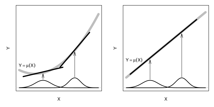
Figure 2: Illustration of the dependence of the population OLS solution on the marginal distribution of the regressors: The left figure shows dependence in the presence of nonlinearity; the right figure shows independence in the presence of linearity.

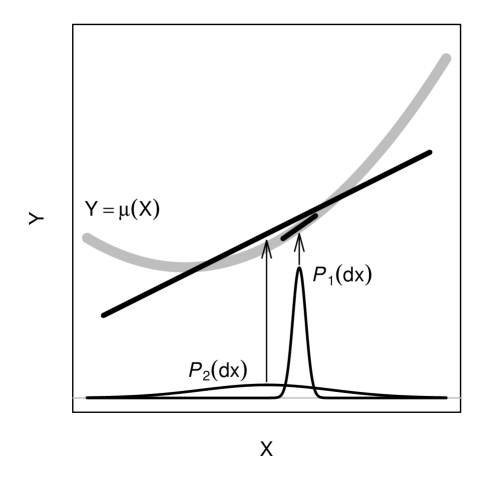
Figure 3: Illustration of the interplay between regressors’ high-density range and nonlinearity: Over the small range of ${\boldsymbol{P}}_{\!1}$ the nonlinearity is undetectable and immaterial for realistic sample sizes, whereas over the extended range of ${\boldsymbol{P}}_{\!2}$ the nonlinearity is more likely to be detectable and relevant.

4.2 Implications of the Dependence of Slopes on Regressor Distributions

A first practical implication, illustrated by Figure 2, is that two empirical studies that use the same regressors, the same response, and the same model, may yet estimate different parameter values, ${\boldsymbol{\beta}}({\boldsymbol{P}}_{\!1})\!\neq\!{\boldsymbol{\beta}}({\boldsymbol{P}}_{\!2})$. This possibility arises even if the true response surface $\mu({\vec{\boldsymbol{x}}})$ is identical between the studies. The reason is model misspecification and differences between the regressor distributions in the two studies. Here is therefore a potential cause of so-called “parameter heterogeneity” in meta-analyses. — The single-regressor situation of Figure 2 gives only an insufficient impression of the problem because for a single regressor such differences between regressor distributions are easily detected. For multiple regressors the differences take on a multivariate nature and may become undetectable.

A second practical implication, illustrated by Figure 3, is that misspecification is a function of the regressor range: Over a narrow range a model has a better chance of appearing “correctly specified.” In the figure the narrow range of ${\boldsymbol{P}}_{\!1}(d{\vec{\boldsymbol{x}}})$ makes the linear approximation appear very nearly correctly specified, whereas the wide range of ${\boldsymbol{P}}_{\!2}(d{\vec{\boldsymbol{x}}})$ results in gross misspecification. Again, the issue gets magnified for larger numbers of regressors where the notion of “regressor range” takes on a multivariate meaning.

Finally, the fact that all models have limited ranges of “acceptable approximation” is a universal issue. This holds even in those physical sciences that are based on the most successful theories known to us.

5 The Noise-Nonlinearity Depomposition of OLS Estimates

We turn to estimation from iid data. We denote iid observations from a joint distribution ${\boldsymbol{P}_{\!\!Y,{\vec{\boldsymbol{X}}}}}$ by $(Y_{i},{\vec{\boldsymbol{X}}}_{i}{{}^{\prime}\,})=(Y_{i},1,X_{i,1},...,~{}X_{i,p})$ ($i=1$, $2$, …, $N$). We stack them to vectors and matrices as in Table 3, inserting a constant 1 in the regressors to accommodate an intercept term. In particular, ${\vec{\boldsymbol{X}}_{\!i}}{{}^{\prime}\,}$ is the $i$’th row and ${{\mathbb{X}}_{\!j}}$ the $j$’th column of the regressor matrix ${\mathbb{X}}$ ($i=1,...,N,~{}j=0,...,p$).

$$\begin{array}[]{|lclclll|}\hline\cr~{}~{}~{}~{}{\boldsymbol{\beta}}&=&(\beta_{0},\beta_{1},...,\beta_{p}){{}^{\prime}\,},&&&\hbox{ parameter vector }&((p+1)\!\times\!1)\\ ~{}~{}~{}~{}{\mathbb{Y}}&=&(Y_{1},...,Y_{N}){{}^{\prime}\,},&&&\hbox{ response vector }&(N\!\times\!1)\\ ~{}~{}~{}~{}{{\mathbb{X}}_{\!j}}&=&(X_{1,j},...,X_{N,j}){{}^{\prime}\,},&&&\hbox{ $j$'th regressor vector }&(N\!\times\!1)\\ ~{}~{}~{}~{}{\mathbb{X}}&=&[{\boldsymbol{1}},{{\mathbb{X}}_{\!1}},...,{{\mathbb{X}}_{\!p}}]&=&\left[\begin{array}[]{c}~{}~{}{\vec{\boldsymbol{X}}_{\!1}}{{}^{\prime}{}{}}\\ .....\\ .....\\ {\vec{\boldsymbol{X}}_{\!N}}{{}^{\prime}}\end{array}\right],&\begin{array}[]{l}\hbox{ regressor matrix }\\ \hbox{ ~{}~{}with intercept }\end{array}&(N\!\times\!(p+1)){}\\ ~{}~{}~{}~{}{\boldsymbol{\mu}}&=&(\mu_{1},...,\mu_{N}){{}^{\prime}\,},&&\mu_{i}=\mu({\vec{\boldsymbol{X}}_{\!i}})={\boldsymbol{E}}[Y|{\vec{\boldsymbol{X}}_{\!i}}],&\hbox{ conditional means }&(N\!\times\!1)\\ ~{}~{}~{}~{}{\boldsymbol{\eta}}&=&({\eta}_{1},...,{\eta}_{N}){{}^{\prime}\,},&&{\eta}_{i}={\eta}({\vec{\boldsymbol{X}}_{\!i}})=\mu_{i}-{\boldsymbol{\beta}}{{}^{\prime}\,}{\vec{\boldsymbol{X}}_{\!i}},&\hbox{ nonlinearities }&(N\!\times\!1)\\ ~{}~{}~{}~{}{\boldsymbol{\epsilon}}&=&({\epsilon}_{1},...,{\epsilon}_{N}){{}^{\prime}\,},&&{\epsilon}_{i}=Y_{i}-\mu_{i},&\hbox{ noise values }&(N\!\times\!1)\\ ~{}~{}~{}~{}{\boldsymbol{\delta}}&=&({\delta}_{1},...,{\delta}_{N}){{}^{\prime}\,},&&{\delta}_{i}={\eta}_{i}+{\epsilon}_{i},&\hbox{ population residuals }&(N\!\times\!1)\\ ~{}~{}~{}~{}{\boldsymbol{\sigma}}&=&({\sigma}_{1},...,{\sigma}_{\!N}){{}^{\prime}\,},&&{\sigma}_{i}={\sigma}({\vec{\boldsymbol{X}}_{\!i}})={\boldsymbol{V}}[Y|{\vec{\boldsymbol{X}}_{\!i}}]^{1/2},&\hbox{ conditional sdevs }&(N\!\times\!1){}{}\\ ~{}~{}~{}~{}{\boldsymbol{\hat{\beta}}}&=&({\hat{\beta}}_{0},{\hat{\beta}}_{1},...,{\hat{\beta}}_{p}){{}^{\prime}}&=&({\mathbb{X}}{{}^{\prime}\,}\!{\mathbb{X}})^{-1}{\mathbb{X}}{{}^{\prime}\,}{\mathbb{Y}}\,,&\hbox{ parameter estimates }&((p+1)\!\times\!1)\\ ~{}~{}~{}~{}{\boldsymbol{r}}&=&(r_{1},...,r_{N}){{}^{\prime}}&=&{\mathbb{Y}}-{\mathbb{X}}{\boldsymbol{\hat{\beta}}},&\hbox{ sample residuals }&(N\!\times\!1)\\ \hline\cr\end{array}$$

Table 3: Random variable notation for estimation in linear OLS based on iid observational data.

The nonlinearity ${\eta}$, the noise ${\epsilon}$, and the population residuals ${\delta}$ generate random $N$-vectors when evaluated at all $N$ observations (again, see Table 3):

$${\boldsymbol{\eta}}~{}=~{}{\boldsymbol{\mu}}\!-\!{\mathbb{X}}{\boldsymbol{\beta}},~{}~{}~{}~{}~{}~{}~{}~{}{\boldsymbol{\epsilon}}~{}=~{}{\mathbb{Y}}\!-\!{\boldsymbol{\mu}},~{}~{}~{}~{}~{}~{}~{}~{}{\boldsymbol{\delta}}~{}=~{}{\mathbb{Y}}\!-\!{\mathbb{X}}{\boldsymbol{\beta}}~{}=~{}{\boldsymbol{\eta}}+{\boldsymbol{\epsilon}}.$$ (9)

It is important to distinguish between population and sample properties: The vectors ${\boldsymbol{\delta}}$, ${\boldsymbol{\epsilon}}$ and ${\boldsymbol{\eta}}$ are not orthogonal to the regressor columns ${{\mathbb{X}}_{\!j}}$ in the sample. Writing $\langle\cdot,\cdot\rangle$ for the usual Euclidean inner product on ${\mathrm{I}\!\mathrm{R}}^{N}$, we have in general

$$\langle{\boldsymbol{\delta}},{{\mathbb{X}}_{\!j}}\rangle~{}\neq~{}0,~{}~{}~{}~{}\langle{\boldsymbol{\epsilon}},{{\mathbb{X}}_{\!j}}\rangle~{}\neq~{}0,~{}~{}~{}~{}\langle{\boldsymbol{\eta}},{{\mathbb{X}}_{\!j}}\rangle~{}\neq~{}0,$$

even though the associated random variables are orthogonal to $X_{j}$ in the population: ${\boldsymbol{E}}[\,{\delta}X_{j}]\!=\!0$, ${\boldsymbol{E}}[\,{\epsilon}X_{j}]\!=\!0$, ${\boldsymbol{E}}[\,{\eta}({\vec{\boldsymbol{X}}})X_{j}]\!=\!0$, according to (6).

The OLS estimate of ${\boldsymbol{\beta}({\boldsymbol{P}})}$ is as usual

$$\begin{array}[]{|l|}\hline\cr~{}~{}{\boldsymbol{\hat{\beta}}}~{}=~{}\mathrm{argmin}_{\tilde{\boldsymbol{\beta}}}\,\|{\mathbb{Y}}\!-\!{\mathbb{X}}{\tilde{\boldsymbol{\beta}}}\|^{2}~{}=~{}({\mathbb{X}}{{}^{\prime}\,}\!{\mathbb{X}})^{-1}{\mathbb{X}}{{}^{\prime}\,}{\mathbb{Y}}\,.\\ \hline\cr\end{array}$$ (10)

If we write ${\boldsymbol{\hat{P}}}$ for the empirical distribution of the observations $(Y_{i},{\vec{\boldsymbol{X}}}_{i}{{}^{\prime}\,})$, then ${\boldsymbol{\hat{\beta}}}={\boldsymbol{\beta}}({\boldsymbol{\hat{P}}})$ is the plug-in estimate. Associated is the sample residual vector ${\boldsymbol{r}}={\mathbb{Y}}\!-\!{\mathbb{X}}{\boldsymbol{\hat{\beta}}}$, based on ${\boldsymbol{\hat{\beta}}}$, which is distinct from the population residual vector ${\boldsymbol{\delta}}={\mathbb{Y}}\!-\!{\mathbb{X}}{\boldsymbol{\beta}}$, based on ${\boldsymbol{\beta}}={\boldsymbol{\beta}({\boldsymbol{P}})}$.

In linear models theory which conditions on (or fixes) ${\mathbb{X}}$, the target of estimation is what we may call the “${\mathbb{X}}$-conditional parameter”:

$$\begin{array}[]{|l|}\hline\cr~{}~{}{\boldsymbol{\beta}({\mathbb{X}})}~{}~{}{\overset{\Delta}{=}}~{}~{}{\boldsymbol{E}}[\,{\boldsymbol{\hat{\beta}}}\,|\,{\mathbb{X}}\,]~{}=~{}\mathrm{argmin}_{\boldsymbol{\beta}}\,{\boldsymbol{E}}[\,\|{\mathbb{Y}}\!-\!{\mathbb{X}}{\boldsymbol{\beta}}\|^{2}\,|\,{\mathbb{X}}\,]~{}=~{}({\mathbb{X}}{{}^{\prime}\,}{\mathbb{X}})^{-1}{\mathbb{X}}{{}^{\prime}\,}{\boldsymbol{\mu}}.{}{}\\ \hline\cr\end{array}$$ (11)

In random-${\mathbb{X}}$ theory, on the other hand, the target of estimation is ${\boldsymbol{\beta}({\boldsymbol{P}})}$, while the ${\mathbb{X}}$-conditional parameter ${\boldsymbol{\beta}}({\mathbb{X}})$ is a random vector. The vectors ${\boldsymbol{\hat{\beta}}}={\boldsymbol{\beta}}({\boldsymbol{\hat{P}}})$, ${\boldsymbol{\beta}}({\mathbb{X}})$ and ${\boldsymbol{\beta}({\boldsymbol{P}})}$ lend themselves to the following telescoping decomposition:

$${{\boldsymbol{\hat{\beta}}}-{\boldsymbol{\beta}({\boldsymbol{P}})}}~{}=~{}({\boldsymbol{\hat{\beta}}}-{\boldsymbol{\beta}({\mathbb{X}})})~{}+~{}({\boldsymbol{\beta}({\mathbb{X}})}-{\boldsymbol{\beta}({\boldsymbol{P}})}),$$ (12)

which in turn reflects the decomposition ${\boldsymbol{\delta}}={\boldsymbol{\epsilon}}+{\boldsymbol{\eta}}$:

Definition and Lemma 5: Define “Estimation Offsets” (EOs) as follows:

$$\begin{array}[]{|lllll|}\hline\cr~{}~{}\textit{Total~{}EO}&~{}~{}{\overset{\Delta}{=}{}{}}&{\boldsymbol{\hat{\beta}}}-{\boldsymbol{\beta}({\boldsymbol{P}})}&~{}={}&({\mathbb{X}}{{}^{\prime}\,}\!{\mathbb{X}})^{-1}{\mathbb{X}}{{}^{\prime}\,}{\boldsymbol{\delta}},{}{}\\ ~{}~{}\textit{Noise~{}EO}&~{}~{}{\overset{\Delta}{=}{}{}}&{\boldsymbol{\hat{\beta}}}-{\boldsymbol{\beta}({\mathbb{X}})}&~{}={}&({\mathbb{X}}{{}^{\prime}\,}\!{\mathbb{X}})^{-1}{\mathbb{X}}{{}^{\prime}\,}{\boldsymbol{\epsilon}},{}{}\\ ~{}~{}\textit{Approximation~{}EO}&~{}~{}{\overset{\Delta}{=}{}{}}&{\boldsymbol{\beta}({\mathbb{X}})}-{\boldsymbol{\beta}({\boldsymbol{P}})}&~{}={}&({\mathbb{X}}{{}^{\prime}\,}\!{\mathbb{X}})^{-1}{\mathbb{X}}{{}^{\prime}\,}{\boldsymbol{\eta}}.{}{}\\ \hline\cr\end{array}$$ (13)

The right sides follow from (9), i.e., ${\boldsymbol{\epsilon}}={\mathbb{Y}}\!\!-\!{\boldsymbol{\mu}}$, ${\boldsymbol{\eta}}={\boldsymbol{\mu}}\!-\!{\mathbb{X}}{\boldsymbol{\beta}}$, ${\boldsymbol{\delta}}={\mathbb{Y}}\!\!-\!{\mathbb{X}}{\boldsymbol{\beta}}$, and

$${\boldsymbol{\hat{\beta}}}=({\mathbb{X}}{{}^{\prime}\,}\!{\mathbb{X}})^{-1}{\mathbb{X}}{{}^{\prime}\,}{\mathbb{Y}},~{}~{}~{}~{}{\boldsymbol{E}}[\,{\boldsymbol{\hat{\beta}}}\,|{\mathbb{X}}]=({\mathbb{X}}{{}^{\prime}\,}\!{\mathbb{X}})^{-1}{\mathbb{X}}{{}^{\prime}\,}{\boldsymbol{\mu}},~{}~{}~{}~{}{\boldsymbol{\beta}({\boldsymbol{P}})}=({\mathbb{X}}{{}^{\prime}\,}\!{\mathbb{X}})^{-1}{\mathbb{X}}{{}^{\prime}\,}({\mathbb{X}}{\boldsymbol{\beta}}).$$

The first defines ${\boldsymbol{\hat{\beta}}}$, the second uses ${\boldsymbol{E}}[{\mathbb{Y}}|{\mathbb{X}}]={\boldsymbol{\mu}}$, and the third is a tautology.

Remark: One might be tempted to interpret the approximation EO ${\boldsymbol{\beta}({\mathbb{X}})}\!-\!{\boldsymbol{\beta}({\boldsymbol{P}})}$ as a bias because it is the difference of two targets of estimation. This interpretation is entirely wrong. The approximation EO is a random variable when nonlinearity is present. It will be seen to contribute not a bias but a $N^{-1/2}$ order term to the sampling variability of ${\boldsymbol{\hat{\beta}}}$ (Section 7).

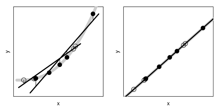
Figure 4: Noise-less Response: The filled and the open circles represent two “datasets” from the same population. The $x$-values are random; the $y$-values are a deterministic function of $x$: $y=\mu(x)$ (shown in gray).
Left: The true response $\mu(x)$ is nonlinear; the open and the filled circles have different OLS lines (shown in black). Right: The true response $\mu(x)$ is linear; the open and the filled circles have the same OLS line (black on top of gray).

6 Broken Regressor Ancillarity II:                     Nonlinearity and Random ${\mathbb{X}}$ Create Sampling Variation

6.1 Sampling Variation’s Two Sources: Noise AND Nonlinearity

For the ${\mathbb{X}}$-conditional parameter ${\boldsymbol{\beta}}({\mathbb{X}})$ to be a non-trivial random variable, two factors need to be present: (1) the regressors ${\vec{\boldsymbol{X}}}$ need to be random and (2) the nonlinearity ${\eta}({\vec{\boldsymbol{X}}})$ must not vanish: ${\boldsymbol{P}}[{\eta}({\vec{\boldsymbol{X}}})\neq 0]>0$. In combination, these factors conspire to produce sampling variation according to (13) which shows the approximation EO to depend on the random matrix $({\mathbb{X}}{{}^{\prime}\,}\!{\mathbb{X}})^{-1}{\mathbb{X}}{{}^{\prime}\,}$ and the vector of nonlinearity values ${\boldsymbol{\eta}}$.

$${\boldsymbol{V}}[\,{\boldsymbol{\hat{\beta}}}\,]~{}=~{}{\boldsymbol{E}}[\,{\boldsymbol{V}}[\,{\boldsymbol{\hat{\beta}}}\,|{\mathbb{X}}]]~{}+~{}{\boldsymbol{V}}[\,{\boldsymbol{E}}[\,{\boldsymbol{\hat{\beta}}}\,|{\mathbb{X}}]]\,,$$ (14)

where the left side represents the full unconditional variability of ${\boldsymbol{\hat{\beta}}}$ relevant for statistical inference. In view of Lemma 5 this decomposition parallels ${\boldsymbol{\delta}}={\boldsymbol{\epsilon}}+{\boldsymbol{\eta}}$:

$$\begin{array}[]{l}\,~{}~{}~{}~{}~{}~{}~{}~{}~{}~{}{\boldsymbol{V}}[\,{\boldsymbol{\hat{\beta}}}\,]~{}=~{}{\boldsymbol{V}}[\,({\mathbb{X}}{{}^{\prime}\,}\!{\mathbb{X}})^{-1}{\mathbb{X}}{{}^{\prime}\,}{\boldsymbol{\delta}}\,]\,,\\ \,~{}~{}{\boldsymbol{E}}[\,{\boldsymbol{V}}[\,{\boldsymbol{\hat{\beta}}}\,|{\mathbb{X}}]]~{}=~{}{\boldsymbol{E}}[\,({\mathbb{X}}{{}^{\prime}\,}\!{\mathbb{X}})^{-1}{\mathbb{X}}{{}^{\prime}\,}\;{\boldsymbol{V}}[\,{\boldsymbol{\epsilon}}\,|{\mathbb{X}}]~{}{\mathbb{X}}\,({\mathbb{X}}{{}^{\prime}\,}\!{\mathbb{X}})^{-1}\,]\\ \begin{array}[]{|l|}\hline\cr~{}~{}{\boldsymbol{V}}[\,{\boldsymbol{E}}[\,{\boldsymbol{\hat{\beta}}}\,|{\mathbb{X}}]\,]~{}=~{}{\boldsymbol{V}}[\,{\boldsymbol{\beta}({\mathbb{X}})}\,]~{}=~{}{\boldsymbol{V}}[\,({\mathbb{X}}{{}^{\prime}\,}\!{\mathbb{X}})^{-1}{\mathbb{X}}{{}^{\prime}\,}{\boldsymbol{\eta}}\,]{}{}\\ \hline\cr\end{array}\end{array}$$ (15)

The center line above the box represents the marginal sampling variability due to noise combined with randomness in ${\mathbb{X}}$. Note that ${\boldsymbol{V}}[\,{\boldsymbol{\epsilon}}\,|{\mathbb{X}}]=D_{{\boldsymbol{\sigma}}^{2}}$ is the diagonal matrix of noise variances. The box shows how the vector of nonlinearities ${\boldsymbol{\eta}}$ “conspires” with the randomness of ${\mathbb{X}}$ to generate sampling variability in ${\boldsymbol{\beta}({\mathbb{X}})}$.

Intuition for the sampling variability of ${\boldsymbol{\beta}({\mathbb{X}})}$ is best provided by a graphical illustration. In order to isolate this effect we consider a noise-free situation where the response is deterministic and nonlinear, hence a linear fit is “misspecified.” To this end let $Y\!=\!\mu({\vec{\boldsymbol{X}}})$ where $\mu(\cdot)$ is some non-linear function (that is, ${\boldsymbol{P}_{\!\!Y|{\vec{\boldsymbol{X}}}}}$ are point masses $\delta_{\mu({\vec{\boldsymbol{X}}})}$), and hence ${\boldsymbol{V}}[{\boldsymbol{\hat{\beta}}}|{\mathbb{X}}]={\boldsymbol{0}}$ vanishes a.s. An example is shown in the left hand frame of Figure 4 for a single regressor, with OLS lines fitted to two “datasets” consisting of $N\!=\!5$ regressor values each. The randomness in the regressors causes the fitted line to differ between datasets, hence exhibit sampling variability due to the nonlinearity of the response. This effect is absent in the right hand frame of Figure 4 where the response is linear.

6.2 Quandaries of Fixed-${\mathbb{X}}$ Theory and the Need for Random-${\mathbb{X}}$ Theory

The fixed-${\mathbb{X}}$ approach of linear models theory necessarily assumes correct specification. Its only source of sampling variability is the noise EO ${\boldsymbol{\hat{\beta}}}\!-\!{\boldsymbol{\beta}({\mathbb{X}})}$ arising from the conditional response distribution, ignoring the approximation EO ${\boldsymbol{\beta}({\mathbb{X}})}\!-\!{\boldsymbol{\beta}({\boldsymbol{P}})}$ due to conditioning on ${\mathbb{X}}$. A partial remedy in fixed-${\mathbb{X}}$ theory is to rely on diagnostics to detect lack of fit (misspecification). We emphasize that diagnostics should be part of every regression analysis. In fact, to assist such diagnostics and make them relevant for correctly sized standard errors, we propose in Section 12 a test to identify slopes that may have their usual standard errors invalidated by misspecification. Furthermore, in Part II we propose a misspecification diagnostic for regression parameters.

Data analysts may not stop with negative findings from model diagnostics and instead continue with data-driven model improvement by, for example, transforming variables and adding terms to the fitted equation till the residuals “look right.” However, model improvement based on the data can have drawbacks and limits. A drawback is that it can invalidate subsequent inferences in unpredictable ways, as does any data-driven variable selection, formal or informal (see, e.g., Berk et al. 2013; Lee et al. 2016). A limit is that residual diagnostics lose power as the number of regressors increases. This fact follows from what we may call “Mammen’s dilemma.” Mammen (1996) showed, roughly speaking, that for models with numerous regressors the residual distribution tends to look as assumed by the working model, e.g., Gaussian for OLS, Laplacian for LAD, irrespective of the true error distribution. For these reasons, data analysts who diagnose and improve their models will find themselves torn at some point between hunches of having done too much of a good thing and missing out on something.

In light of such uncertainties arising from diagnostics and model improvement, it may be of some comfort that tools are available for asymptotically correct inference under model misspecification, including misspecified deterministic responses ($Y\!=\!\mu({\vec{\boldsymbol{X}}}),~{}\sigma^{2}({\vec{\boldsymbol{X}}})\!=\!0)$. These tools — sandwich and ${x\textrm{-}y}$ bootstrap estimators of standard error — derive their justification from central limit theorems (CLTs) to be described next.

7 Model-Robust CLTs, Canonically Decomposed

Random-${\mathbb{X}}$ CLTs for OLS are standard, and the novel aspect of the following proposition is in decomposing the overall asymptotic variance into contributions stemming from the noise EO and the approximation EO according to (13), thereby providing an asymptotic analog of the finite-sample decomposition of sampling variance in Section 6.1.

Proposition 7: For linear OLS the three EOs follow CLTs:

$$\begin{array}[]{|rcl|}\hline\cr\sqrt{N}\,({\boldsymbol{\hat{\beta}}}-{\boldsymbol{\beta}})\!\!&\stackrel{{\scriptstyle{\cal D}}}{{\longrightarrow}}&\!\!{\cal N}\left({\boldsymbol{0}},{\boldsymbol{E}}[{\vec{\boldsymbol{X}}}{\vec{\boldsymbol{X}}}{{}^{\prime}\,}]^{-1}\,{\boldsymbol{E}}[\,{m}^{2}({\vec{\boldsymbol{X}}}){\vec{\boldsymbol{X}}}{\vec{\boldsymbol{X}}}{{}^{\prime}\,}]\;{\boldsymbol{E}}[{\vec{\boldsymbol{X}}}{\vec{\boldsymbol{X}}}{{}^{\prime}\,}]^{-1}\right)\\ \sqrt{N}\,({\boldsymbol{\hat{\beta}}}-{\boldsymbol{\beta}({\mathbb{X}})})\!\!&\stackrel{{\scriptstyle{\cal D}}}{{\longrightarrow}}&\!\!{\cal N}\left({\boldsymbol{0}},{\boldsymbol{E}}[{\vec{\boldsymbol{X}}}{\vec{\boldsymbol{X}}}{{}^{\prime}\,}]^{-1}\,{\boldsymbol{E}}[\,{\sigma}^{2}({\vec{\boldsymbol{X}}}){\vec{\boldsymbol{X}}}{\vec{\boldsymbol{X}}}{{}^{\prime}\,}]\;{\boldsymbol{E}}[{\vec{\boldsymbol{X}}}{\vec{\boldsymbol{X}}}{{}^{\prime}\,}]^{-1}\right)\\ \sqrt{N}\,({\boldsymbol{\beta}({\mathbb{X}})}-{\boldsymbol{\beta}})\!\!&\stackrel{{\scriptstyle{\cal D}}}{{\longrightarrow}}&\!\!{\cal N}\left({\boldsymbol{0}},{\boldsymbol{E}}[{\vec{\boldsymbol{X}}}{\vec{\boldsymbol{X}}}{{}^{\prime}\,}]^{-1}\,{\boldsymbol{E}}[\,{\eta}^{2}({\vec{\boldsymbol{X}}}){\vec{\boldsymbol{X}}}{\vec{\boldsymbol{X}}}{{}^{\prime}\,}]\;{\boldsymbol{E}}[{\vec{\boldsymbol{X}}}{\vec{\boldsymbol{X}}}{{}^{\prime}\,}]^{-1}\right)\\ \hline\cr\end{array}$$ (16)

These three statements once again reflect the decomposition (8), ${m}^{2}({\vec{\boldsymbol{X}}})=$ ${\sigma}^{2}({\vec{\boldsymbol{X}}})+$ ${\eta}^{2}({\vec{\boldsymbol{X}}})$. According to (7) and (8), ${m}^{2}({\vec{\boldsymbol{X}}})$ can be replaced by ${\delta}^{2}$ and ${\sigma}^{2}({\vec{\boldsymbol{X}}})$ by ${\epsilon}^{2}$:

$${\boldsymbol{E}}[\,{m}^{2}({\vec{\boldsymbol{X}}}){\vec{\boldsymbol{X}}}{\vec{\boldsymbol{X}}}{{}^{\prime}\,}]~{}=~{}{\boldsymbol{E}}[\,{\delta}^{2}{\vec{\boldsymbol{X}}}{\vec{\boldsymbol{X}}}{{}^{\prime}\,}],~{}~{}~{}~{}{\boldsymbol{E}}[\,\sigma^{2}({\vec{\boldsymbol{X}}}){\vec{\boldsymbol{X}}}{\vec{\boldsymbol{X}}}{{}^{\prime}\,}]~{}=~{}{\boldsymbol{E}}[\,{\epsilon}^{2}{\vec{\boldsymbol{X}}}{\vec{\boldsymbol{X}}}{{}^{\prime}\,}].$$ (17)

The asymptotic variance of linear OLS can therefore be written as

$$\begin{array}[]{l}{\boldsymbol{A\!V}}[{\boldsymbol{P}};{\boldsymbol{\beta}}]~{}~{}{\overset{\Delta}{=}}~{}~{}{\boldsymbol{E}}[{\vec{\boldsymbol{X}}}{\vec{\boldsymbol{X}}}{{}^{\prime}\,}]^{-1}\,{\boldsymbol{E}}[\,{\delta}^{2}{\vec{\boldsymbol{X}}}{\vec{\boldsymbol{X}}}{{}^{\prime}\,}]\,{\boldsymbol{E}}[{\vec{\boldsymbol{X}}}{\vec{\boldsymbol{X}}}{{}^{\prime}\,}]^{-1}\,.\end{array}$$ (18)

As always, ${\boldsymbol{\beta}}$ stands for the statistical functional ${\boldsymbol{\beta}}={\boldsymbol{\beta}}({\boldsymbol{P}})$ and by implication its plug-in OLS estimator ${\boldsymbol{\hat{\beta}}}={\boldsymbol{\beta}}({\boldsymbol{\hat{P}}})$. The formula is the basis for plug-in that produces the sandwich estimator of standard error (Section 8.1).

Special cases covered by the above proposition are the following:

• First order correct specification:  ${\eta}({\vec{\boldsymbol{X}}})\overset{{\boldsymbol{P}}}{=}0$. The sandwich form is solely due to heteroskedasticity.

• Deterministic nonlinear response:  ${\sigma}^{2}({\vec{\boldsymbol{X}}})\overset{{\boldsymbol{P}}}{=}0$. The sandwich form is solely due to the nonlinearity and randomness of ${\mathbb{X}}$.

• First and second order correct specification: ${\eta}({\vec{\boldsymbol{X}}})\!\overset{{\boldsymbol{P}}}{=}\!0$, ${\sigma}^{2}({\vec{\boldsymbol{X}}})\!\overset{{\boldsymbol{P}}}{=}\!{\sigma}_{0}^{2}$. The non-sandwich form is asymptotically valid without Gaussianity: $\sqrt{N}\,({\boldsymbol{\hat{\beta}}}-{\boldsymbol{\beta}})~{}\stackrel{{\scriptstyle{\cal D}}}{{\longrightarrow}}~{}{\cal N}\left({\boldsymbol{0}},~{}{\sigma}_{0}^{2}\,{\boldsymbol{E}}[\,{\vec{\boldsymbol{X}}}{\vec{\boldsymbol{X}}}{{}^{\prime}\,}]^{-1}\right)$.

8 Sandwich Estimators and the $M$-of-$N$ Bootstrap

Empirically one observes that standard error estimates obtained from the ${x\textrm{-}y}$ bootstrap and from the sandwich estimator are generally close to each other (Section 2). This is intuitively unsurprising as they both estimate the same asymptotic variance, that of the first CLT in Proposition 7. A closer connection between them will be described here and established in generality in Part II (Buja et al. 2018).

8.1 The Plug-In Sandwich Estimator of Asymptotic Variance

Plug-in estimators of standard error are obtained by substituting the empirical distribution ${\boldsymbol{\hat{P}}}$ for the true ${\boldsymbol{P}}$ in formulas for asymptotic variances. As the asymptotic variance ${\boldsymbol{A\!V}}[{\boldsymbol{P}};{\boldsymbol{\beta}}]$ in (18) is given explicitly and also suitably continuous in the two arguments, one obtains a consistent estimator by plugging in ${\boldsymbol{\hat{P}}}$ for ${\boldsymbol{P}}$:

$${{\boldsymbol{\hat{A\!V}}\!\!}}\,[\,{\boldsymbol{\beta}}\,]~{}~{}{\overset{\Delta}{=}}~{}~{}{\boldsymbol{A\!V}}[{\boldsymbol{\beta}},{\boldsymbol{\hat{P}}}],~{}~{}~{}~{}~{}~{}~{}{\boldsymbol{\hat{{S\!E}}}}[{\beta_{j}}]~{}~{}{\overset{\Delta}{=}}~{}~{}\frac{1}{N^{1/2}}({{\boldsymbol{\hat{A\!V}}\!\!}}\,[\,{\boldsymbol{\beta}}\,])_{jj}^{~{}1/2}.$$ (19)

[Recall again that ${\boldsymbol{\beta}}\!=\!{\boldsymbol{\beta}}({\boldsymbol{P}})$ stands for the OLS statistical functional which specializes to its plug-in estimator through ${\boldsymbol{\hat{\beta}}}={\boldsymbol{\beta}}({\boldsymbol{\hat{P}}})$.] Concretely, one estimates expectations ${\boldsymbol{E}}[...]$ with sample means $\boldsymbol{\hat{E}}[...]$, ${\boldsymbol{\beta}}={\boldsymbol{\beta}}({\boldsymbol{P}})$ with ${\boldsymbol{\hat{\beta}}}={\boldsymbol{\beta}}({\boldsymbol{\hat{P}}})$, and hence population residuals ${\delta}^{2}=(Y\!-\!{\vec{\boldsymbol{X}}}{\boldsymbol{\beta}})^{2}$ with sample residuals $r_{i}^{2}=(Y_{i}\!-\!{\vec{\boldsymbol{X}}_{\!i}}{\boldsymbol{\hat{\beta}}})^{2}$. Collecting the latter in a diagonal matrix ${\boldsymbol{D}}_{\boldsymbol{r}}^{2}$, one has

$$\begin{array}[]{ccc}\boldsymbol{\hat{E}}[\,r^{2}\,{\vec{\boldsymbol{X}}}{\vec{\boldsymbol{X}}}{{}^{\prime}\,}]=\frac{1}{N}\,({\mathbb{X}}{{}^{\prime}\,}{\boldsymbol{D}}_{\boldsymbol{r}}^{2}\,{\mathbb{X}}),&{}{}{}{}\hfil&\boldsymbol{\hat{E}}[\,{\vec{\boldsymbol{X}}}{\vec{\boldsymbol{X}}}{{}^{\prime}\,}]=\frac{1}{N}\,({\mathbb{X}}{{}^{\prime}\,}\!{\mathbb{X}}).\end{array}$$

The sandwich estimator ${{\boldsymbol{\hat{A\!V}}\!\!\!}_{sand}}[\,{\boldsymbol{\beta}}\,]={{\boldsymbol{\hat{A\!V}}\!\!}}\,[\,{\boldsymbol{\beta}}\,]$ for linear OLS in its original form (White 1980a) is therefore obtained explicitly as follows:

$$\begin{array}[]{rcl}{{\boldsymbol{\hat{A\!V}}\!\!\!}_{sand}}[\,{\boldsymbol{\beta}}\,]&{\overset{\Delta}{=}}&\boldsymbol{\hat{E}}[\,{\vec{\boldsymbol{X}}}{\vec{\boldsymbol{X}}}{{}^{\prime}\,}]^{-1}\,\boldsymbol{\hat{E}}[\,r^{2}{\vec{\boldsymbol{X}}}{\vec{\boldsymbol{X}}}{{}^{\prime}\,}]\;\boldsymbol{\hat{E}}[\,{\vec{\boldsymbol{X}}}{\vec{\boldsymbol{X}}}{{}^{\prime}\,}]^{-1}\\[8.0pt] &=&N\,({\mathbb{X}}{{}^{\prime}\,}\!{\mathbb{X}})^{-1}\,({\mathbb{X}}{{}^{\prime}\,}{\boldsymbol{D}}_{\boldsymbol{r}}^{2}\,{\mathbb{X}})\,({\mathbb{X}}{{}^{\prime}\,}\!{\mathbb{X}})^{-1}\end{array}$$ (20)

This is version “HC” in MacKinnon and White (1985). A modification accounts for the fact that residuals have smaller variance than noise, calling for a correction by replacing $1/N^{1/2}$ in (19) with $1/(N\!-\!p\!-\!1)^{1/2}$, in analogy to the linear models estimator (“HC1” ibid.). Another modification is to correct individual residuals for their reduced variance according to ${\boldsymbol{V}}[r_{i}|{\mathbb{X}}]={\sigma}^{2}(1-H_{ii})$ under homoskedasticity and ignoring nonlinearity (“HC2” ibid.). Further modifications include a version based on the jackknife (“HC3” ibid.) using leave-one-out residuals. MacKinnon and White (1985) also mention that some forms of sandwich estimators were independently derived by Efron (1982, p. 18f) using the infinitesimal jackknife, and by Hinkley (1977) using a “weighted jackknife.” See Weber (1986) for a concise comparison in the linear model limited to heteroskedasticity.

8.2 Sandwich Estimators are Limits of $M$-of-$N$ Bootstrap Estimators

An alternative to plug-in is estimating asymptotic variance with the ${x\textrm{-}y}$ bootstrap whose justification essentially derives from the validity of the CLT . Conventionally the resample size, here denoted by $M$, is taken to be the same as the sample size $N$, but it is useful to distinguish between these two quantities and allow the resample size $M$ to differ from $N$, resulting in the “$M$-of-$N$ bootstrap.” One distinguishes

• $M$-of-$N$ bootstrap resampling with replacement from

• $M$-out-of-$N$ subsampling without replacement.

In resampling, $M$ can be any $M\!<\!\infty$; in subsampling, $M$ must satisfy $M\!<\!N$. To fix notation, denote bootstrap estimates by ${{\boldsymbol{\beta}^{*}}}_{\!\!\!M}\!=\!{\boldsymbol{\beta}}({\boldsymbol{P}}_{\!\!M}^{*})$, where ${\boldsymbol{P}}_{\!\!M}^{*}$ is the empirical distribution of bootstrap data $\{(Y_{i}^{*},{\vec{\boldsymbol{X}}_{\!i}}^{*}{{}^{\prime}\,})\}_{i=1...M}$ drawn iid from ${\boldsymbol{\hat{P}}}_{\!\!N}$. Bootstrap estimates of asymptotic variance are therefore

$${{\boldsymbol{\hat{A\!V}}\!\!}_{boot}}[\,{\boldsymbol{\beta}}\,] {\overset{\Delta}{=}} M\,{\boldsymbol{V}}_{\!\!\!{\boldsymbol{\hat{P}}}_{\!\!N}}[\,{{\boldsymbol{\beta}^{*}}}_{\!\!\!M}\,].$$ (21)

The connection between bootstrap and sandwich estimates is as follows:

Proposition 8.2: The sandwich estimator (20) is the $M$-of-$N$ bootstrap estimator (21) in the limit $M\!\!\rightarrow\!\infty$ for a fixed sample of size $N$.

See Part II (Buja et al. 2018) for full generality. Bootstrap approaches may be more flexible than sandwich approaches because the bootstrap distribution can be used to generate confidence intervals that are second order correct (see, e.g., Efron and Tibshirani 1994; Hall 1992; McCarthy, Zhang et. al. 2016).

9 Adjusted Regressors

This section prepares the ground for two projects: (1) proposing meanings of slopes in the presence of nonlinearity (Section 10), and (2) comparing standard errors of slopes, model-robust versus model-trusting (Section 11). The first requires the well-known adjustment formula for slopes in multiple regression, while the second requires adjustment formulas for standard errors, both model-trusting and model-robust. Although the adjustment formulas are standard, they will be stated explicitly to fix notation. [See Appendix D for more notational details.]

• Adjustment in Populations: The population-adjusted regressor random variable ${X_{\!j{\scriptscriptstyle\bullet}}}$ is the “residual” of the population regression of ${{X}_{\!j}}$, used as the response, on all other regressors. The response $Y$ can be adjusted similarly, and we may denote it by $Y_{\!{\scriptscriptstyle\bullet}\,{{\!\scriptscriptstyle-}\!j}}$ to indicate that $X_{j}$ is not among the adjustors, which is implicit in the adjustment of $X_{j}$. The multiple regression coefficient ${\beta_{j}}={\beta_{j}}({\boldsymbol{P}})$ of the population regression of $Y$ on ${\vec{\boldsymbol{X}}}$ is obtained as the simple regression through the origin of $Y_{\!{\scriptscriptstyle\bullet}\,{{\!\scriptscriptstyle-}\!j}}$ or $Y$ on ${X_{\!j{\scriptscriptstyle\bullet}}}$:

  $${\beta_{j}}~{}=~{}\frac{{\boldsymbol{E}}[\,Y_{\!{\scriptscriptstyle\bullet}\,{{\!\scriptscriptstyle-}\!j}}{X_{\!j{\scriptscriptstyle\bullet}}}]}{{\boldsymbol{E}}[\,{X_{\!j{\scriptscriptstyle\bullet}}^{\,2}}]}~{}=~{}\frac{{\boldsymbol{E}}[\,Y{X_{\!j{\scriptscriptstyle\bullet}}}]}{{\boldsymbol{E}}[\,{X_{\!j{\scriptscriptstyle\bullet}}^{\,2}}]}~{}=~{}\frac{{\boldsymbol{E}}[\,\mu({\vec{\boldsymbol{X}}}){X_{\!j{\scriptscriptstyle\bullet}}}]}{{\boldsymbol{E}}[\,{X_{\!j{\scriptscriptstyle\bullet}}^{\,2}}]}\,.$$ (22)

  The rightmost representation holds because ${X_{\!j{\scriptscriptstyle\bullet}}}$ is a function of ${\vec{\boldsymbol{X}}}$ only which permits conditioning of $Y$ on ${\vec{\boldsymbol{X}}}$ in the numerator.

• Adjustment in Samples: Define the sample-adjusted regressor column ${{\mathbb{X}}_{\!j{\hat{\scriptscriptstyle\bullet}}}}$ to be the residual vector of the sample regression of ${{\mathbb{X}}_{\!j}}$, used as the response vector, on all other regressors. The response vector ${\mathbb{Y}}$ can be sample-adjusted similarly, and we may denote it by ${{\mathbb{Y}}_{\!\!{\hat{\scriptscriptstyle\bullet}}\,{{\!\scriptscriptstyle-}\!j}}}$ to indicate that ${{\mathbb{X}}_{\!j}}$ is not among the adjustors, which is implicit for ${{\mathbb{X}}_{\!j{\hat{\scriptscriptstyle\bullet}}}}$. (Note the use of hat notation “$\,{\hat{\scriptscriptstyle\bullet}}\,$” to distinguish it from population-based adjustment “${\scriptscriptstyle\bullet}$.”) The coefficient estimate ${\hat{\beta}_{j}}$ of the multiple regression of ${\mathbb{Y}}$ on ${\mathbb{X}}$ is obtained as the simple regression through the origin of ${{\mathbb{Y}}_{\!\!{\hat{\scriptscriptstyle\bullet}}\,{{\!\scriptscriptstyle-}\!j}}}$ or ${\mathbb{Y}}$ on ${{\mathbb{X}}_{\!j{\scriptscriptstyle\bullet}}}$:

  $${\hat{\beta}_{j}}~{}=~{}\frac{\langle{{\mathbb{Y}}_{\!\!{\hat{\scriptscriptstyle\bullet}}\,{{\!\scriptscriptstyle-}\!j}}},{{\mathbb{X}}_{\!j{\hat{\scriptscriptstyle\bullet}}}}\rangle}{\|{{\mathbb{X}}_{\!j{\hat{\scriptscriptstyle\bullet}}}}\|^{2}}~{}=~{}\frac{\langle{\mathbb{Y}},{{\mathbb{X}}_{\!j{\hat{\scriptscriptstyle\bullet}}}}\rangle}{\|{{\mathbb{X}}_{\!j{\hat{\scriptscriptstyle\bullet}}}}\|^{2}}\,.$$ (23)

[For practice, the patient reader may wrap his/her mind around the distinction between ${{\mathbb{X}}_{\!j{\hat{\scriptscriptstyle\bullet}}}}$ and ${{\mathbb{X}}_{\!j{\scriptscriptstyle\bullet}}}$, the latter being the vector of population-adjusted ${X_{i,j{\scriptscriptstyle\bullet}}}$. The components of the former are dependent, those of the latter independent.]

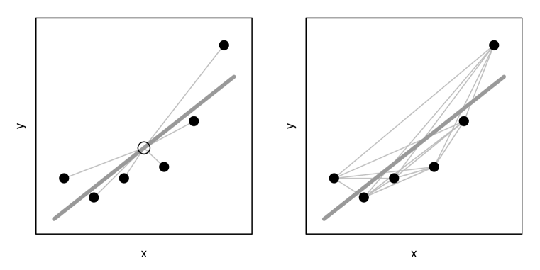
Figure 5: Case-wise and pairwise average weighted slopes illustrated: Both plots show the same six points (“cases”) as well as the OLS line fitted to them (fat gray). The left hand plot shows the case-wise slopes from the mean point (open circle) to the six cases, while the right hand plot shows the pairwise slopes between all 15 pairs. In both plots the observed slopes are positive with just one exception each, supporting the impression that the direction of association is positive.

10 Meanings of Slopes in the Presence of Nonlinearity

A first use of regressor adjustment is for proposing meanings of linear slopes in the presence of nonlinearity, and responding to Freedman’s (2006, p. 302) objection: “… it is quite another thing to ignore bias [nonlinearity]. It remains unclear why applied workers should care about the variance of an estimator for the wrong parameter.” Against this view one may argue that “flawed” models are a fact of life. Flaws such as nonlinearity can go undetected, or they can be tolerated for insightful simplification. A “parameter” based on best approximation is then not intrinsically wrong but in need of a useful interpretation.

The issue is that, in the presence of nonlinearity, slopes lose their usual interpretation: ${\beta_{j}}$ is no longer the average difference in $Y$ associated with a unit difference in $X_{j}$ at fixed levels of all other $X_{k}$. Such an interpretation holds for the best approximation ${\boldsymbol{\beta}}^{\prime}{\vec{\boldsymbol{x}}}$ but not the conditional mean function $\mu({\vec{\boldsymbol{x}}})$. The challenge is to provide an alternative interpretation that remains valid and intuitive. As mentioned, a plausible approach is to use adjusted variables, hence by (22) and (23) it is sufficient to solve the interpretation problem for simple regression through the origin. In a sense to be made precise, slopes can then be interpreted as weighted averages of “case-wise” and “pairwise” slopes. — To lighten the notational burden, we drop subscripts from adjusted variables:

$$y\leftarrow{Y_{\!{\scriptscriptstyle\bullet}\,{{\!\scriptscriptstyle-}\!j}}}\,,~{}~{}~{}~{}~{}~{} x\leftarrow{X_{\!j{\scriptscriptstyle\bullet}}}\,,\,~{}~{}~{}~{}~{}~{}~{}~{}\beta\leftarrow{\beta_{j}}\,~{}~{}~{}~{}\textrm{for populations,}$$

$$y_{i}\leftarrow({{\mathbb{Y}}_{\!\!{\hat{\scriptscriptstyle\bullet}}\,{{\!\scriptscriptstyle-}\!j}}})_{i}\,,~{}~{} x_{i}\leftarrow({{\mathbb{X}}_{\!j{\hat{\scriptscriptstyle\bullet}}}})_{i}\,,~{}~{}~{}~{}{\hat{\beta}}\leftarrow{\hat{\beta}_{j}}~{}~{}~{}~{}\textrm{for samples.}$$

By (22) and (23), the population slopes and their estimates are, respectively,

$$\beta=\frac{E[yx]}{E[x^{2}]}~{}~{}~{}~{}~{}~{}\textrm{and}~{}~{}~{}~{}~{}~{}{\hat{\beta}}=\frac{\sum y_{i}x_{i}}{\sum x_{i}^{2}}.$$

Slope interpretation will be based on the following devices:

• Population parameters $\beta$ can be represented as weighted averages of …

  • case-wise slopes: For a random case $(x,y)$ we have

    $$\beta={\boldsymbol{E}}[\,w\,b\,],~{}~{}~{}\textrm{where}~{}~{}~{}b~{}{\overset{\Delta}{=}}~{}\frac{y}{x},~{}~{}~{}~{}w~{}{\overset{\Delta}{=}}~{}\frac{x^{2}}{{\boldsymbol{E}}[\,x^{2}\,]}.$$

    Thus $b$ is the case-wise slope through the origin and $w$ its weight.

  • pairwise slopes: For iid cases $(x,y)$ and $(x^{\prime},y^{\prime})$ we have

    $$\beta~{}=~{}{\boldsymbol{E}}[\,w\,b\,],~{}~{}~{}\textrm{where}~{}~{}~{}b~{}{\overset{\Delta}{=}}~{}\frac{y-y^{\prime}}{x-x^{\prime}},~{}~{}~{}~{}w~{}{\overset{\Delta}{=}}~{}\frac{(x-x^{\prime})^{2}}{{\boldsymbol{E}}[\,(x-x^{\prime})^{2}\,]}.$$

    Thus $b$ is the pairwise slope and $w$ its weight.

• Sample estimates ${\hat{\beta}}$ can be represented as weighted averages of …

  • case-wise slopes:

    $${\hat{\beta}}=\sum_{i}\,w_{i}\,b_{i}\,,~{}~{}~{}\textrm{where}~{}~{}~{}b_{i}~{}{\overset{\Delta}{=}}~{}\frac{y_{i}}{x_{i}},~{}~{}~{}~{}w_{i}~{}{\overset{\Delta}{=}}~{}\frac{x_{i}^{2}}{\sum_{i^{\prime}}\,x_{i^{\prime}}^{2}\,}.$$

    Thus $b_{i}$ are case-wise slopes and $w_{i}$ their weights.

  • pairwise slopes:

    $${\hat{\beta}}=\sum_{ik}\,w_{ik}\,b_{ik}\,,~{}~{}~{}\textrm{where}~{}~{}~{}b_{ik}~{}{\overset{\Delta}{=}}~{}\frac{y_{i}-y_{k}}{x_{i}-x_{k}},~{}~{}~{}~{}w_{ik}~{}{\overset{\Delta}{=}}~{}\frac{(x_{i}-x_{k})^{2}}{\sum_{i^{\prime}k^{\prime}}\,(x_{i^{\prime}}-x_{k^{\prime}})^{2}\,}.$$

    Thus $b_{ik}$ are pairwise slopes and $w_{ik}$ their weights ($i\neq k$).

See Figure 5 for an illustration for samples. The formulas support the intuition that, even in the presence of nonlinearity, a linear fit can describe the overall direction of the association between the response and a regressor after adjustment.

There exist of course examples where no global direction of association exists, as when ${\boldsymbol{E}}[y|x]\!\sim\!x^{2}$ and the regressor distribution ${\boldsymbol{P}}_{\!\!x}$ is symmetric about $0$. The association is local, negative for $x<0$ and positive for $x>0$. But if ${\boldsymbol{E}}[x]/{\boldsymbol{S\!D}}[x]\gg 0$, the direction of association is positive, and a linear fit provides an excellent approximation to $x^{2}$, illustrating once again the crucial role of ${\boldsymbol{P}}_{\!\!x}$.

We conclude with a note on the history of the above formulas: Stigler (2001) points to Edgeworth, while Berman (1988) traces them back to an 1841 article by Jacobi written in Latin. A generalization based on tuples rather than pairs of cases was used by Wu (1986) for the analysis of jackknife and bootstrap procedures (see his Section 3, Theorem 1). Gelman and Park (2008) also refer to the representation of OLS slopes as weighted means of pairwise slopes.

11 Asymptotic Variances — Proper and Improper

The following prepares the ground for an asymptotic comparison of model-robust and model-trusting standard errors, one regressor at a time.

11.1 Preliminaries: Adjustment Formulas for EOs and Their CLTs:

The vectorized formulas for estimation offsets (12) can be written componentwise using adjustment as follows:

$$\begin{array}[]{|lrcl|}\hline\cr\textit{~{}Total~{}EO}:&{\hat{\beta}_{j}}-{\beta_{j}}&=&\displaystyle\frac{\langle{{\mathbb{X}}_{\!j{\hat{\scriptscriptstyle\bullet}}}},{\boldsymbol{\delta}}\rangle}{\|{{\mathbb{X}}_{\!j{\hat{\scriptscriptstyle\bullet}}}}\|^{2}},{}\\[2.0pt] \textit{~{}Noise~{}EO}:&{\hat{\beta}_{j}}-{\beta_{j}}({\mathbb{X}})&=&\displaystyle\frac{\langle{{\mathbb{X}}_{\!j{\hat{\scriptscriptstyle\bullet}}}},{\boldsymbol{\epsilon}}\rangle}{\|{{\mathbb{X}}_{\!j{\hat{\scriptscriptstyle\bullet}}}}\|^{2}},{}\\[2.0pt] \textit{~{}Approximation~{}EO}:{}{}{}&{\beta_{j}}({\mathbb{X}})-{\beta_{j}}&=&\displaystyle\frac{\langle{{\mathbb{X}}_{\!j{\hat{\scriptscriptstyle\bullet}}}},{\boldsymbol{\eta}}\rangle}{\|{{\mathbb{X}}_{\!j{\hat{\scriptscriptstyle\bullet}}}}\|^{2}}.{}\\[6.0pt] \hline\cr\end{array}$$ (24)

To see these identities directly, note the following, in addition to (23): ${\boldsymbol{E}}[{\hat{\beta}_{j}}|{\mathbb{X}}]=\langle{\boldsymbol{\mu}},{{\mathbb{X}}_{\!j{\hat{\scriptscriptstyle\bullet}}}}\rangle/\|{{\mathbb{X}}_{\!j{\hat{\scriptscriptstyle\bullet}}}}\|^{2}$ and ${\beta_{j}}=\langle{\mathbb{X}}{\boldsymbol{\beta}},{{\mathbb{X}}_{\!j{\hat{\scriptscriptstyle\bullet}}}}\rangle/\|{{\mathbb{X}}_{\!j{\hat{\scriptscriptstyle\bullet}}}}\|^{2}$, the latter due to $\langle{{\mathbb{X}}_{\!j{\hat{\scriptscriptstyle\bullet}}}},{\mathbb{X}}_{k}\rangle=\delta_{jk}\|{{\mathbb{X}}_{\!j{\hat{\scriptscriptstyle\bullet}}}}\|^{2}$. Finally use ${\boldsymbol{\delta}}={\mathbb{Y}}\!-\!{\mathbb{X}}{\boldsymbol{\beta}}$, ${\boldsymbol{\eta}}={\boldsymbol{\mu}}\!-\!{\mathbb{X}}{\boldsymbol{\beta}}$ and ${\boldsymbol{\epsilon}}={\mathbb{Y}}\!-\!{\boldsymbol{\mu}}$.  $\square$

From (24), asymptotic normality of the coefficient-specific EOs can be separately expressed using population adjustment:

Corollary 11.1:

$$\begin{array}[]{|ccccc|}\hline\cr~{}~{}N^{1/2}({\hat{\beta}_{j}}-{\beta_{j}})&\stackrel{{\scriptstyle{\cal D}}}{{\longrightarrow}}&\displaystyle{\cal N}\left(0,\frac{{\boldsymbol{E}}[\,{m}^{2}({\vec{\boldsymbol{X}}}){X_{\!j{\scriptscriptstyle\bullet}}^{\,2}}]}{{\boldsymbol{E}}[\,{X_{\!j{\scriptscriptstyle\bullet}}^{\,2}}]^{2}}\right)&=&\displaystyle{\cal N}\left(0,\frac{{\boldsymbol{E}}[\,{\delta}^{2}{X_{\!j{\scriptscriptstyle\bullet}}^{\,2}}]}{{\boldsymbol{E}}[\,{X_{\!j{\scriptscriptstyle\bullet}}^{\,2}}]^{2}}\right){}\\[16.0pt] ~{}~{}N^{1/2}({\hat{\beta}_{j}}-{\beta_{j}}({\mathbb{X}}))&\stackrel{{\scriptstyle{\cal D}}}{{\longrightarrow}}&\displaystyle{\cal N}\left(0,\frac{{\boldsymbol{E}}[\,\sigma^{2}({\vec{\boldsymbol{X}}}){X_{\!j{\scriptscriptstyle\bullet}}^{\,2}}]}{{\boldsymbol{E}}[\,{X_{\!j{\scriptscriptstyle\bullet}}^{\,2}}]^{2}}\right)&=&\displaystyle{\cal N}\left(0,\frac{{\boldsymbol{E}}[\,{\epsilon}^{2}{X_{\!j{\scriptscriptstyle\bullet}}^{\,2}}]}{{\boldsymbol{E}}[\,{X_{\!j{\scriptscriptstyle\bullet}}^{\,2}}]^{2}}\right)\\[16.0pt] ~{}N^{1/2}({\beta_{j}}({\mathbb{X}})-{\beta_{j}})&\stackrel{{\scriptstyle{\cal D}}}{{\longrightarrow}}&\displaystyle{\cal N}\left(0,\frac{{\boldsymbol{E}}[\,{\eta}^{2}({\vec{\boldsymbol{X}}}){X_{\!j{\scriptscriptstyle\bullet}}^{\,2}}]}{{\boldsymbol{E}}[\,{X_{\!j{\scriptscriptstyle\bullet}}^{\,2}}]^{2}}\right)&&\\[6.0pt] \hline\cr\end{array}$$

The equalities on the right side in the first and second case are based on (17). The first CLT in its right side form is useful for plug-in estimation of asymptotic variance, one slope at a time. The sandwich form of matrices has been reduced to ratios where numerators correspond to the “meat” and squared denominators to the “breads.”

11.2 Model-Robust Asymptotic Variances in Terms of Adjusted Regressors:

The CLTs of Corollary 11.1 contain three asymptotic variances of the same form with arguments ${m}^{2}({\vec{\boldsymbol{X}}})$, ${\sigma}^{2}({\vec{\boldsymbol{X}}})$ and ${\eta}^{2}({\vec{\boldsymbol{X}}})$. We will use ${m}^{2}({\vec{\boldsymbol{X}}})$ in the following definition for the overall asymptotic variance, but by substituting ${\sigma}^{2}({\vec{\boldsymbol{X}}})$ or ${\eta}^{2}({\vec{\boldsymbol{X}}})$ for ${m}^{2}({\vec{\boldsymbol{X}}})$ one obtains terms that can be interpreted as components of the overall asymptotic variance or else as asymptotic variances in the absence of nonlinearity or absence of noise.

Definition 11.2: Proper Asymptotic Variance.

$$\begin{array}[]{|c|}\hline\cr\vspace{-.13in}\hfil\\ {\boldsymbol{A\!V}_{\!\!{{lean}}}}[{\beta_{j}};{m}^{2}]~{}~{}{\overset{\Delta}{=}}~{}~{}\displaystyle\frac{{\boldsymbol{E}}[\,{m}^{2}({\vec{\boldsymbol{X}}}){X_{\!j{\scriptscriptstyle\bullet}}^{\,2}}]}{{\boldsymbol{E}}[\,{X_{\!j{\scriptscriptstyle\bullet}}^{\,2}}]^{2}}.\\[10.00002pt] \hline\cr\end{array}$$

From (8), ${m}^{2}({\vec{\boldsymbol{X}}})\!=\!{\sigma}^{2}({\vec{\boldsymbol{X}}})\!+\!{\eta}^{2}({\vec{\boldsymbol{X}}})$, one obtains

$${\boldsymbol{A\!V}_{\!\!{{lean}}}}[{\beta_{j}};{m}^{2}]~{}=~{}{\boldsymbol{A\!V}_{\!\!{{lean}}}}[{\beta_{j}};{\sigma}^{2}]+{\boldsymbol{A\!V}_{\!\!{{lean}}}}[{\beta_{j}};{\eta}^{2}].$$

The subscript “${{lean}}$” refers to validity in the assumption-lean model-robust framework. This proper asymptotic variance will be compared to the potentially improper asymptotic variance of model-trusting linear models theory (Section 11.4).

11.3 Model-Trusting Asymptotic Variances in Terms of Adjusted Regressors

The goal is to provide an asymptotic limit for the usual model-trusting standard error estimate of linear models theory in the model-robust framework. To this end we need the model-robust limit of the usual estimate of the noise variance, ${\hat{\sigma}}^{2}=\|{\mathbb{Y}}-{\mathbb{X}}{\boldsymbol{\hat{\beta}}}\|^{2}/(N\!-\!p\!-\!1)$:

$${\hat{\sigma}}^{2}~{}~{}\overset{{\boldsymbol{P}}}{\longrightarrow}~{}~{}{\boldsymbol{E}}[\,{\delta}^{2}\,]~{}=~{}{\boldsymbol{E}}[\,{m}^{2}({\vec{\boldsymbol{X}}})\,]~{}=~{}{\boldsymbol{E}}[\,{\sigma}^{2}({\vec{\boldsymbol{X}}})\,]+{\boldsymbol{E}}[\,{\eta}^{2}({\vec{\boldsymbol{X}}})\,],~{}~{}~{}~{}~{}~{}N\rightarrow\infty.$$

Thus the model-robust limit of ${\hat{\sigma}}^{2}$ is the average conditional MSE of $Y$, which again decomposes according to ${m}^{2}({\vec{\boldsymbol{X}}})\!=\!{\sigma}^{2}({\vec{\boldsymbol{X}}})\!+\!{\eta}^{2}({\vec{\boldsymbol{X}}})$.

Squared standard error estimates are, in matrix and adjustment form,

$$\boldsymbol{\hat{V}}_{{\!\!\!lin}}[\,{\boldsymbol{\hat{\beta}}}\,]~{}=~{}{\hat{\sigma}}^{2}\,({\mathbb{X}}{{}^{\prime}\,}\!{\mathbb{X}})^{-1},~{}~{}~{}~{}~{}~{}~{}~{}{\boldsymbol{\hat{{S\!E}}}}^{2}_{{\!\!\>l\!\!\;i\!\!\;n}}[\,{\hat{\beta}}]~{}=~{}\frac{{\hat{\sigma}}^{2}}{\|{{\mathbb{X}}_{\!j{\hat{\scriptscriptstyle\bullet}}}}\|^{2}}.$$ (25)

Their assumption-lean scaled limits are

$$N\,\boldsymbol{\hat{V}}_{{\!\!\!lin}}[\,{\boldsymbol{\hat{\beta}}}\,]~{}\overset{{\boldsymbol{P}}}{\longrightarrow}~{}{\boldsymbol{E}}[\,{m}^{2}({\vec{\boldsymbol{X}}})\,]~{}{\boldsymbol{E}}[\,{\vec{\boldsymbol{X}}}{\vec{\boldsymbol{X}}}{{}^{\prime}\,}\,]^{-1},~{}~{}~{}~{}~{}N\,{\boldsymbol{\hat{{S\!E}}}}^{2}_{{\!\!\>l\!\!\;i\!\!\;n}}[\,{\hat{\beta}_{j}}]~{}\overset{{\boldsymbol{P}}}{\longrightarrow}~{}\frac{{\boldsymbol{E}}[\,{m}^{2}({\vec{\boldsymbol{X}}})\,]}{{\boldsymbol{E}}[\,X_{j{\scriptscriptstyle\bullet}}^{2}\,]}.$$

Definition 11.3 Improper Asymptotic Variance.

$$\begin{array}[]{|c|}\hline\cr\vspace{-.13in}\hfil\\ {\boldsymbol{A\!V}_{\!\!{{\!\!\>l\!\!\;i\!\!\;n}}}}[{\beta_{j}};{m}^{2}]~{}~{}{\overset{\Delta}{=}}~{}~{}\displaystyle\frac{{\boldsymbol{E}}[\,{m}^{2}({\vec{\boldsymbol{X}}})]}{{\boldsymbol{E}}[\,{X_{\!j{\scriptscriptstyle\bullet}}^{\,2}}]}.\\[10.00002pt] \hline\cr\end{array}$$

This decomposes once again according to ${m}^{2}({\vec{\boldsymbol{X}}})\!=\!{\sigma}^{2}({\vec{\boldsymbol{X}}})\!+\!{\eta}^{2}({\vec{\boldsymbol{X}}})$:

$${\boldsymbol{A\!V}_{\!\!{{\!\!\>l\!\!\;i\!\!\;n}}}}[{\beta_{j}};{m}^{2}]~{}=~{}{\boldsymbol{A\!V}_{\!\!{{\!\!\>l\!\!\;i\!\!\;n}}}}[{\beta_{j}};{\sigma}^{2}]+{\boldsymbol{A\!V}_{\!\!{{\!\!\>l\!\!\;i\!\!\;n}}}}[{\beta_{j}};{\eta}^{2}].$$

The subscript  ${{\!\!\>l\!\!\;i\!\!\;n}}$ refers to validity of this asymptotic variance under the assumption-loaded model-trusting framework of linear models theory.

11.4 ${\boldsymbol{R\!A\!V}}$ — Ratio of Proper and Improper Asymptotic Variances

To examine the discrepancies between proper and improper asymptotic variances we form their ratio, which results in the following elegant functional of the conditional MSE and the squared adjusted regressor:

Definition 11.4:  Ratio of Asymptotic Variances (${\boldsymbol{R\!A\!V}}\!$), Proper/Improper.

$$\begin{array}[]{|ccccc|}\hline\cr{\boldsymbol{R\!A\!V}}[{\beta_{j}},{m}^{2}]&{\overset{\Delta}{=}}&\displaystyle\frac{{\boldsymbol{A\!V}_{\!\!{{lean}}}}[{\beta_{j}},{m}^{2}]}{{\boldsymbol{A\!V}_{\!\!{{\!\!\>l\!\!\;i\!\!\;n}}}}[{\beta_{j}},{m}^{2}]}&=&\displaystyle\frac{{\boldsymbol{E}}[{m}^{2}({\vec{\boldsymbol{X}}}){X_{\!j{\scriptscriptstyle\bullet}}^{\,2}}]}{{\boldsymbol{E}}[{m}^{2}({\vec{\boldsymbol{X}}})]\,{\boldsymbol{E}}[{X_{\!j{\scriptscriptstyle\bullet}}^{\,2}}]}.\\[8.99994pt] \hline\cr\end{array}$$

In order to examine the effect of heteroskedasticities and nonlinearities on the discrepancies separately, one can also define ${\boldsymbol{R\!A\!V}}[{\beta_{j}},{\sigma}^{2}]$ and ${\boldsymbol{R\!A\!V}}[{\beta_{j}},{\eta}^{2}]$. By the decomposition lemma in Appendix E.2, ${\boldsymbol{R\!A\!V}}[{\beta_{j}},{m}^{2}]$ is a weighted mixture of these two terms. — Belaboring the obvious, the interpretation of the ${\boldsymbol{R\!A\!V}}$ is:

$$\textrm{If~{}~{}}{\boldsymbol{R\!A\!V}}[{\beta_{j}},{m}^{2}]\left\{\begin{array}[]{c}>1\\ =1\\ <1\end{array}\right\},\textrm{then~{}}{\boldsymbol{\hat{{S\!E}}}}_{{\!\!\>l\!\!\;i\!\!\;n}}[{\hat{\beta}_{j}}]\textrm{~{}is~{}asymptotically~{}}\left\{\begin{array}[]{l}\textrm{too~{}small}\\ \textrm{correct}\\ \textrm{too~{}large}\end{array}\right\}.$$

We will later have use for the following sufficient condition for ${\boldsymbol{R\!A\!V}}\!=\!1$. It says essentially that when the population residual ${\delta}$ is a traditional error term, then the usual standard error of linear models theory is asymptotically correct. The condition is equivalent to first and second order correct specification, including linearity and homoskedasticity but not Gaussianity.

Lemma 11.4: Sufficient conditions for ${\boldsymbol{R\!A\!V}}[{\beta_{j}},{m}^{2}]=1$ are the following:

• ${m}^{2}({\vec{\boldsymbol{X}}})={m}_{0}^{2}$ is constant.

• ${\delta}^{2}$ and ${X_{\!j{\scriptscriptstyle\bullet}}}^{2}$ are independent.

Proof: $(a)$ is immediate from Definition 11.4. $(b)$ The numerator of ${\boldsymbol{R\!A\!V}}[{\beta_{j}},{m}^{2}]$ is ${\boldsymbol{E}}[{m}^{2}({\vec{\boldsymbol{X}}}){X_{\!j{\scriptscriptstyle\bullet}}}^{2}]\!=\!{\boldsymbol{E}}[\,{\delta}^{2}{X_{\!j{\scriptscriptstyle\bullet}}}^{2}]\!=\!{\boldsymbol{E}}[\,{\delta}^{2}]\,{\boldsymbol{E}}[{X_{\!j{\scriptscriptstyle\bullet}}}^{2}]$, hence equals the denominator. $\square$

The ratio ${\boldsymbol{R\!A\!V}}[{\beta_{j}},{m}^{2}]$ is the inner product between the random variables

$$\frac{{m}^{2}({\vec{\boldsymbol{X}}})}{{\boldsymbol{E}}[{m}^{2}({\vec{\boldsymbol{X}}})]}~{}~{}~{}~{}\mbox{and}~{}~{}~{}~{}\frac{{X_{\!j{\scriptscriptstyle\bullet}}^{\,2}}}{{\boldsymbol{E}}[{X_{\!j{\scriptscriptstyle\bullet}}^{\,2}}]}.$$

It is not a correlation as both ${m}^{2}({\vec{\boldsymbol{X}}})$ and ${X_{\!j{\scriptscriptstyle\bullet}}^{\,2}}$ are $L_{1}$-normalized; a non-centered correlation would require $L_{2}$-normalization with denominators ${\boldsymbol{E}}[{m}^{4}({\vec{\boldsymbol{X}}})]^{1/2}$ and ${\boldsymbol{E}}[{X_{\!j{\scriptscriptstyle\bullet}}^{\,4}}]^{1/2}$, respectively. Its upper bound is obviously not $+1$ but rather $\infty$:

11.5 The Range of ${\boldsymbol{R\!A\!V}}$

The analysis of the ${\boldsymbol{R\!A\!V}}$ is simplified by conditioning ${m}^{2}({\vec{\boldsymbol{X}}})$ on ${X_{\!j{\scriptscriptstyle\bullet}}^{\,2}}$:

Definition and Lemma 11.5: Letting

$${m}_{j}^{2}({X_{\!j{\scriptscriptstyle\bullet}}^{\,2}})~{}~{}{\overset{\Delta}{=}}~{}~{}{\boldsymbol{E}}[{m}^{2}({\vec{\boldsymbol{X}}})\,|\,{X_{\!j{\scriptscriptstyle\bullet}}^{\,2}}],$$

we have:

$${\boldsymbol{R\!A\!V}}[{\beta_{j}},{m}^{2}]~{}=~{}{\boldsymbol{R\!A\!V}}[{\beta_{j}},{m}_{j}^{2}].$$

Thus the analysis of the ${\boldsymbol{R\!A\!V}}$ is reduced to single squared adjusted regressors ${X_{\!j{\scriptscriptstyle\bullet}}^{\,2}}$. This fact lends itself to simple case studies and graphical illustrations.

Next we describe the extremes of the ${\boldsymbol{R\!A\!V}}$ over scenarios of ${m}^{2}({\vec{\boldsymbol{X}}})$ or, by Lemma 11.5, of ${m}_{j}^{2}({X_{\!j{\scriptscriptstyle\bullet}}^{\,2}})$.

Proposition 11.5: If ${\boldsymbol{E}}[{X_{\!j{\scriptscriptstyle\bullet}}^{\,2}}]<\infty$ and ${X_{\!j{\scriptscriptstyle\bullet}}^{\,2}}$ has unbounded support, then

$$\sup_{{m}_{j}^{2}}{\boldsymbol{R\!A\!V}}[{\beta_{j}},{m}_{j}^{2}]~{}=~{}\infty.$$

If ${\boldsymbol{E}}[{X_{\!j{\scriptscriptstyle\bullet}}^{\,2}}]<\infty$ and ${X_{\!j{\scriptscriptstyle\bullet}}^{\,2}}$ has 0 in its support, then

$$\inf_{{m}_{j}^{2}}{\boldsymbol{R\!A\!V}}[{\beta_{j}},{m}_{j}^{2}]~{}=~{}0.$$

Figure 6: A family of functions $f_{t}^{2}(x)$ that can be interpreted as conditional MSEs ${m}_{j}^{2}({X_{\!j{\scriptscriptstyle\bullet}}^{\,2}})$, heteroskedasticities $\sigma_{j}^{2}({X_{\!j{\scriptscriptstyle\bullet}}^{\,2}})$ or squared nonlinearities ${\eta}_{j}^{2}({X_{\!j{\scriptscriptstyle\bullet}}^{\,2}})$ (shown as functions of $x={X_{\!j{\scriptscriptstyle\bullet}}}$ rather than ${X_{\!j{\scriptscriptstyle\bullet}}^{\,2}}$): The family interpolates ${\boldsymbol{R\!A\!V}}$ from $0$ to $\infty$ for $x={X_{\!j{\scriptscriptstyle\bullet}}}\sim N(0,1)$. The three solid black curves show $f_{t}^{2}(x)$ that result in RAV=0.05, 1, and 10. (See Appendix E.4 for details.)
${\boldsymbol{R\!A\!V}}=\infty$ is approached as $f_{t}^{2}(x)$ bends ever more strongly in the tails of the $x$-distribution.
${\boldsymbol{R\!A\!V}}=0$ is approached by an ever stronger spike in the center of the $x$-distribution.

Figure 7: The effect of heteroskedasticity on the sampling variability of slope estimates: How does the treatment of the heteroskedasticities as homoskedastic affect statistical inference?
Left: High noise variance in the tails of the regressor distribution elevates the true sampling variability of the slope estimate above the usual standard error: ${\boldsymbol{R\!A\!V}}[{\beta_{j}},{\sigma}^{2}]>1$.
Center: High noise variance near the center of the regressor distribution lowers the true sampling variability of the slope estimate below the usual standard error: ${\boldsymbol{R\!A\!V}}[{\beta_{j}},{\sigma}^{2}]<1$.
Right: The noise variance oscillates in such a way that the usual standard error is coincidentally correct (${\boldsymbol{R\!A\!V}}[{\beta_{j}},{\sigma}^{2}]=1$).

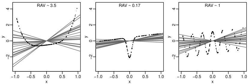
Figure 8: The effect of nonlinearities on the sampling variability of slope estimates: The three plots show three different noise-free nonlinearities; each plot shows for one nonlinearity 20 overplotted datasets of size $N=10$ and their fitted lines through the origin. The question is how the misinterpretation of the nonlinearities as homoskedastic random errors affects statistical inference.
Left: Strong nonlinearity in the tails of the regressor distribution elevates the true sampling variability of the slope estimate above the usual standard error (${\boldsymbol{R\!A\!V}}[{\beta_{j}},{\eta}^{2}]>1$).
Center: Strong nonlinearity near the center of the regressor distribution lowers the true sampling variability of the slope estimate below the usual standard error (${\boldsymbol{R\!A\!V}}[{\beta_{j}},{\eta}^{2}]<1$).
Right: An oscillating nonlinearity mimics homoskedastic random error to make the usual standard error coincidentally correct (${\boldsymbol{R\!A\!V}}[{\beta_{j}},{\eta}^{2}]=1$).
Caveat: These are cartoons illustrating potential causes of standard error discrepancies. Nonlinearities may not be detectable in actual data in the presence of noise and other regressors.

Thus, when the adjusted regressor distribution is unbounded, the usual standard error can be too small to any degree. Conversely, if the adjusted regressor is not bounded away from zero, it can be too large to any degree.

What shapes of ${m}_{j}^{2}({X_{\!j{\scriptscriptstyle\bullet}}^{\,2}})$ approximate these extremes? The answer can be gleaned from Figure 6 which illustrates the proposition for normally distributed ${X_{\!j{\scriptscriptstyle\bullet}}}$: If nonlinearities and/or heteroskedasticities blow up …

• in the tails of the ${X_{\!j{\scriptscriptstyle\bullet}}}$ distribution, then ${\boldsymbol{R\!A\!V}}$ takes on large values;

• in the center of the ${X_{\!j{\scriptscriptstyle\bullet}}}$ distribution, then ${\boldsymbol{R\!A\!V}}$ takes on small values.

The proof in Appendix E.3 bears this out. As the main concern is with usual standard errors that are too small, ${\boldsymbol{R\!A\!V}}\!>\!1$, the proposition indicates that ${X_{\!j{\scriptscriptstyle\bullet}}}$-distributions with bounded support enjoy some protection from the worst case.

11.6 Illustration of Factors that Drive the ${\boldsymbol{R\!A\!V}}$

We further analyze the ${\boldsymbol{R\!A\!V}}\!$ in terms of the constituents of ${m}_{j}^{2}({X_{\!j{\scriptscriptstyle\bullet}}^{\,2}})$, conditional variance and squared nonlinearity, as functions of ${X_{\!j{\scriptscriptstyle\bullet}}^{\,2}}$:

$${\sigma}_{j}^{2}({X_{\!j{\scriptscriptstyle\bullet}}^{\,2}})={\boldsymbol{E}}[{\sigma}^{2}({\vec{\boldsymbol{X}}})|{X_{\!j{\scriptscriptstyle\bullet}}^{\,2}}]~{}~{}~{}~{}\textrm{and}~{}~{}~{}~{}{\eta}_{j}^{2}({X_{\!j{\scriptscriptstyle\bullet}}^{\,2}})={\boldsymbol{E}}[{\eta}^{2}({\vec{\boldsymbol{X}}})|{X_{\!j{\scriptscriptstyle\bullet}}^{\,2}}].$$ (26)

For qualitative insights into the drivers of the ${\boldsymbol{R\!A\!V}}\!\!$, we translate (26) to concrete data scenarios. Figure 7 shows three noise scenarios and Figure 8 three nonlinearity scenarios. The illustrated effects will both be present to degrees in real data. Their combined effect is described by a decomposition lemma in Appendix E.2: ${\boldsymbol{R\!A\!V}}[{\beta_{j}},{m}_{j}^{2}]$ is a weighted mixture of ${\boldsymbol{R\!A\!V}}[{\beta_{j}},{\sigma}_{j}^{2}]$ and ${\boldsymbol{R\!A\!V}}[{\beta_{j}},{\eta}_{j}^{2}]$. Therefore:

• Heteroskedasticities with large ${\sigma}_{j}^{2}({X_{\!j{\scriptscriptstyle\bullet}}^{\,2}})$ in the tails of ${X_{\!j{\scriptscriptstyle\bullet}}}^{2}$ produce an upward contribution to ${\boldsymbol{R\!A\!V}}[{\beta_{j}},{m}_{j}^{2}]$; heteroskedasticities with large ${\sigma}_{j}^{2}({X_{\!j{\scriptscriptstyle\bullet}}^{\,2}})$ near ${X_{\!j{\scriptscriptstyle\bullet}}^{\,2}}=0$ imply a downward contribution to ${\boldsymbol{R\!A\!V}}[{\beta_{j}},{m}_{j}^{2}]$.

• Nonlinearities with large average values ${\eta}_{j}^{2}({X_{\!j{\scriptscriptstyle\bullet}}^{\,2}})$ in the tails of ${X_{\!j{\scriptscriptstyle\bullet}}^{\,2}}$ imply an upward contribution to ${\boldsymbol{R\!A\!V}}[{\beta_{j}},{m}_{j}^{2}]$; nonlinearities with large ${\eta}_{j}^{2}({X_{\!j{\scriptscriptstyle\bullet}}^{\,2}})$ concentrated near ${X_{\!j{\scriptscriptstyle\bullet}}^{\,2}}=0$ imply a downward contribution to ${\boldsymbol{R\!A\!V}}[{\beta_{j}},{m}_{j}^{2}]$.

These facts also suggest that large values ${\boldsymbol{R\!A\!V}}\!\!>\!1$ should occur more often than small values ${\boldsymbol{R\!A\!V}}\!\!<\!1$ because large conditional variances as well as nonlinearities are often more pronounced in the extremes of regressor distributions, not their centers. This is most natural for nonlinearities which are often convex or concave. Also, it follows from the ${\boldsymbol{R\!A\!V}}\!$ decomposition lemma (Appendix E.2) that either of ${\boldsymbol{R\!A\!V}}[{\beta_{j}},\sigma_{j}^{2}]$ or ${\boldsymbol{R\!A\!V}}[{\beta_{j}},{\eta}_{j}^{2}]$ is able to single-handedly pull ${\boldsymbol{R\!A\!V}}[{\beta_{j}},{m}_{j}^{2}]$ to $+\infty$, whereas both have to be close to zero to pull ${\boldsymbol{R\!A\!V}}[{\beta_{j}},{m}_{j}^{2}]$ toward zero. These heuristics support the observation that in practice ${\boldsymbol{\hat{{S\!E}}}}_{{\!\!\>l\!\!\;i\!\!\;n}}$ is more often too small than too large compared to the asymptotically correct ${\boldsymbol{\hat{{S\!E}}}}_{{\!\!\>s\!\!\>a\!\!\>n\!\!\>d}}$.

12 Sandwich Estimators in Adjusted Form and a ${\boldsymbol{R\!A\!V}}$ Test

The goal here is to write the ${\boldsymbol{R\!A\!V}}$ in adjustment form and estimate it with plug-in for use as a test statistic to decide whether the usual standard error is adequate. We will obtain one test per regressor. The proposal is related to the class of “misspecification tests” for which there exists a literature starting with Hausman (1978) and continuing with White (1980a,b; 1981; 1982) and others. These tests are largely global rather than coefficient-specific, which ours is. The test proposed here has similarities to White’s (1982, Section 4) “information matrix test” which compares two types of information matrices globally, while we compare two types of standard errors, one coefficient at a time.

12.1 Sandwich Estimators in Adjustment Form and the ${\boldsymbol{\hat{R\!A\!V}}_{\!\!j}}$ Test Statistic

The adjustment versions of the asymptotic variances in the CLTs of Corollary 11.1 can be used to rewrite the sandwich estimator by replacing expectations ${\boldsymbol{E}}[...]$ with means $\boldsymbol{\hat{E}}[...]$, ${\boldsymbol{\beta}}$ with ${\boldsymbol{\hat{\beta}}}$, ${X_{\!j{\scriptscriptstyle\bullet}}}$ with ${{\mathbb{X}}_{\!j{\hat{\scriptscriptstyle\bullet}}}}$, and rescaling by $N$:

$${\boldsymbol{\hat{{S\!E}}}}_{{{\!\!\>s\!\!\>a\!\!\>n\!\!\>d}}}[{\hat{\beta}_{j}}]^{2}~{}=~{}\frac{1}{N}\frac{\boldsymbol{\hat{E}}[\,(Y-{\vec{\boldsymbol{X}}}{{}^{\prime}\,}{\boldsymbol{\hat{\beta}}})^{2}{X_{\!j{\hat{\scriptscriptstyle\bullet}}}}^{2}]}{\boldsymbol{\hat{E}}[\,{X_{\!j{\hat{\scriptscriptstyle\bullet}}}}^{2}]^{\,2}}~{}=~{}\frac{\langle{\boldsymbol{r}}^{2},{{\mathbb{X}}_{\!j{\hat{\scriptscriptstyle\bullet}}}}^{2}\rangle}{\|{{\mathbb{X}}_{\!j{\hat{\scriptscriptstyle\bullet}}}}\|^{4}}.$$ (27)

The squaring of $N$-vectors is meant to be coordinate-wise. Formula (27) is algebraically equivalent to the diagonal elements of (20).

To match the raw plug-in form of the sandwich estimator (27), we use the plug-in version of the standard error estimator of linear models theory, the only difference being division by $N$ rather than $N\!-\!p\!-\!1$:

$${\boldsymbol{\hat{{S\!E}}}}_{{{\!\!\>l\!\!\;i\!\!\;n}}}[{\hat{\beta}_{j}}]^{2}~{}=~{}\frac{1}{N}\frac{\boldsymbol{\hat{E}}[(Y-{\vec{\boldsymbol{X}}}{{}^{\prime}\,}{\boldsymbol{\hat{\beta}}})^{2}]}{\boldsymbol{\hat{E}}[{X_{\!j{\hat{\scriptscriptstyle\bullet}}}}^{2}]}~{}=~{}\frac{1}{N}\frac{\|{\boldsymbol{r}}\|^{2}}{\|{{\mathbb{X}}_{\!j{\hat{\scriptscriptstyle\bullet}}}}\|^{2}}\,,$$ (28)

Thus the plug-in estimate of ${\boldsymbol{R\!A\!V}}[{\beta_{j}},{m}^{2}]$ is

$${\boldsymbol{\hat{R\!A\!V}}_{\!\!j}}~{}~{}{\overset{\Delta}{=}}~{}~{}\frac{\boldsymbol{\hat{E}}[\,(Y-{\vec{\boldsymbol{X}}}{{}^{\prime}\,}{\boldsymbol{\hat{\beta}}})^{2}{X_{\!j{\hat{\scriptscriptstyle\bullet}}}}^{2}\,]}{\boldsymbol{\hat{E}}[\,(Y-{\vec{\boldsymbol{X}}}{{}^{\prime}\,}{\boldsymbol{\hat{\beta}}})^{2}\,]\,\boldsymbol{\hat{E}}[\,{X_{\!j{\hat{\scriptscriptstyle\bullet}}}}^{2}\,]}~{}=~{}N\,\frac{\langle{\boldsymbol{r}}^{2},{{\mathbb{X}}_{\!j{\hat{\scriptscriptstyle\bullet}}}}^{2}\rangle}{\|{\boldsymbol{r}}\|^{2}\;\|{{\mathbb{X}}_{\!j{\hat{\scriptscriptstyle\bullet}}}}\|^{2}}\,.$$ (29)

This is the proposed test statistic. Analogous to the population-level ${\boldsymbol{R\!A\!V}}[{\beta_{j}},{m}^{2}]$, the sample-level ${\boldsymbol{\hat{R\!A\!V}}_{\!\!j}}$ responds to associations between squared residuals and squared adjusted regressors.

12.2 The Asymptotic Null Distribution of the ${\boldsymbol{R\!A\!V}}$ Test Statistic

Here is an asymptotic result that would be expected to yield approximate inference under a null hypothesis that implies ${\boldsymbol{R\!A\!V}}[{\beta_{j}},{m}^{2}]=1$ based on Lemma 11.4:

Proposition 12.2:  Under the null hypothesis $H_{0}$ that the population residuals ${\delta}$ and the adjusted regressor ${X_{\!j{\scriptscriptstyle\bullet}}}$ are independent, it holds:

$$N^{1/2}\,({\boldsymbol{\hat{R\!A\!V}}_{\!\!j}}-1)~{}\overset{{\cal D}}{\longrightarrow}~{}{\cal N}\left(0,\,\frac{{\boldsymbol{E}}[\,{\delta}^{4}]}{{\boldsymbol{E}}[\,{\delta}^{2}]^{2}}\,\frac{{\boldsymbol{E}}[{X_{\!j{\scriptscriptstyle\bullet}}}^{4}]}{{\boldsymbol{E}}[{X_{\!j{\scriptscriptstyle\bullet}}^{\,2}}]^{2}}\,-\,1)\right).$$ (30)

As always we ignore technical assumptions. A proof outline is in Appendix E.5.

The asymptotic variance of ${\boldsymbol{\hat{R\!A\!V}}_{\!\!j}}$ under $H_{0}$ is driven by the standardized fourth moments or the kurtoses (= same$\,-\,$3) of ${\delta}$ and ${X_{\!j{\scriptscriptstyle\bullet}}}$. Some observations:

1. The larger the kurtosis of population residuals ${\delta}$ and/or adjusted regressors ${X_{\!j{\scriptscriptstyle\bullet}}}$, the less likely is detection of first and second order model misspecification resulting in standard error discrepancies.

2. As standardized fourth moments are always $\geq 1$ by Jensen’s inequality, the asymptotic variance is $\geq 0$, as it should be. The asymptotic variance vanishes iff the minimal standardized fourth moment is $+1$ for both ${\delta}$ and ${X_{\!j{\scriptscriptstyle\bullet}}}$, hence both have symmetric two-point distributions (as both are centered). For such ${X_{\!j{\scriptscriptstyle\bullet}}}$ it holds ${\boldsymbol{R\!A\!V}}[{\beta_{j}},{m}^{2}]\!=\!1$ by Proposition E.3 in the appendix.

3. A test of the stronger $H_{0}$ that includes normality of ${\delta}$ is obtained by setting ${\boldsymbol{E}}[{\delta}^{4}]/{\boldsymbol{E}}[{\delta}^{2}]^{2}$ $=3$ rather than estimating it. The result, however, is an overly sensitive non-normality test much of the time, which does not seem useful as non-normality can be diagnosed and tested by other means.

	${\hat{\beta}_{j}}$	${\boldsymbol{S\!E}}_{{\!\!\>l\!\!\;i\!\!\;n}}$	${\boldsymbol{S\!E}}_{{\!\!\>s\!\!\>a\!\!\>n\!\!\>d}}$	${\boldsymbol{\hat{R\!A\!V}}_{\!\!j}}$	2.5% Perm.	97.5% Perm.
(Intercept)	0.760	22.767	16.209	0.495	0.354	3.182
MedianIncome ($K)	-0.183	0.187	0.108	0.318	0.274	5.059
PercVacant	4.629	0.901	1.363	2.071	0.303	3.823
PercMinority	0.123	0.176	0.164	0.860	0.403	2.238
PercResidential	-0.050	0.171	0.111	0.406	0.369	3.058
PercCommercial	0.737	0.273	0.397	2.046	0.355	3.073
PercIndustrial	0.905	0.321	0.592	3.289*	0.323	3.215

Table 4: LA Homeless data: Permutation Inference for ${\boldsymbol{\hat{R\!A\!V}}_{\!\!j}}$ (10,000 permutations). The value of ${\boldsymbol{\hat{R\!A\!V}}_{\!\!j}}$ for PercIndustrial detects a statistically significant difference between ${\boldsymbol{S\!E}}_{{\!\!\>l\!\!\;i\!\!\;n}}$ and ${\boldsymbol{S\!E}}_{{\!\!\>s\!\!\>a\!\!\>n\!\!\>d}}$ for this regressor. See also Table 8 in the Appendix for the Boston Housing data where significant differences are detected for 6 of 13 regressors.

12.3 An Approximate Permutation Distribution for the ${\boldsymbol{R\!A\!V}}$ Test Statistic

The asymptotic result of Proposition 12.2 provides qualitative insights, but it is not suitable for practical application because the null distribution of ${\boldsymbol{\hat{R\!A\!V}}_{\!\!j}}$ can be very non-normal for finite $N$, and this in ways that are not easily overcome with simple tools such as nonlinear transformations. Another approach to null distributions for finite $N$ is needed, and it is available in the form of an approximate permutation test because $H_{0}$ is just a null hypothesis of independence, here between ${\delta}$ and ${X_{\!j{\scriptscriptstyle\bullet}}}$. The test is not exact, requiring $N\!\gg\!p$, because population residuals ${\delta}_{i}$ must be estimated with sample residuals $r_{i}$ and population adjusted regressor values ${X_{i,j{\scriptscriptstyle\bullet}}}$ with sample adjusted analogs ${X_{i,j{\hat{\scriptscriptstyle\bullet}}}}$. The permutation simulation is cheap: Once coordinate-wise squared vectors ${\boldsymbol{r}}^{2}$ and ${{\mathbb{X}}_{\!j{\hat{\scriptscriptstyle\bullet}}}}^{2}$ are formed, a draw from the conditional null distribution of ${\boldsymbol{\hat{R\!A\!V}}_{\!\!j}}$ is obtained by randomly permuting one of the vectors and forming the inner product with the other, rescaled by a permutation-invariant factor $N/(\|{\boldsymbol{r}}\|^{2}\|{{\mathbb{X}}_{\!j{\hat{\scriptscriptstyle\bullet}}}}\|^{2})$. A retention interval should be formed directly from the $\alpha/2$ and $1\!-\!\alpha/2$ quantiles of the permutation distribution to account for distributional asymmetries. The permutation distribution also yields an easy diagnostic of non-normality (see Appendix F for examples). Finally, by applying permutation simulations simultaneously to ${\boldsymbol{R\!A\!V}}$ statistics of multiple regressors, one can calibrate the retention intervals to control family-wise error. — See Table 4 (and 8 in the Appendix) for examples of ${\boldsymbol{R\!A\!V}}$ tests.

13 Issues with Model-Robust Standard Errors

Model-robustness is a highly desirable property, but as always there is no free lunch. Kauermann and Carroll (2001) have shown that a cost of the sandwich estimator can be inefficiency when the assumed model is correct. Sandwich estimators should be accurate only when the sample size is sufficiently large.

Another cost associated with the sandwich estimator is non-robustness in the sense of robust statistics (Huber and Ronchetti 2009, Hampel et al. 1986), meaning strong sensitivity to heavy-tailed distributions: The statistic ${\boldsymbol{\hat{{S\!E}}}}_{{\!\!\>s\!\!\>a\!\!\>n\!\!\>d}}^{2}[{\hat{\beta}_{j}}]$ (27) is a ratio of fourth order quantities of the data, whereas ${\boldsymbol{\hat{{S\!E}}}}_{{\!\!\>l\!\!\;i\!\!\;n}}^{2}[{\hat{\beta}_{j}}]$ (28) is “only” a ratio of second order quantities. The two types of robustness are in conflict: Model-robust standard error estimators are highly non-robust to heavy tails compared to their model-trusting analogs. This is a large issue which we can only raise but not solve. Here are some observations and suggestions:

• Classical robust regression may confer partial robustness to the sandwich standard error as it caps residuals with a bounded $\psi$ function, thereby addressing robustness to heavy tails in the vertical ($y$) direction. Anecdotal evidence suggests partial benefits. In the LA Homeless data, for example, when comparing boostrap standard errors and standard errors reported by the R (2008)) software (function lmrob in package robustbase), we observed ratios $\frac{{\boldsymbol{S\!E}}_{{\!\!\>b\!\!\;o\!\!\;o\!\!\;t}}}{{\boldsymbol{S\!E}}_{{\!\!\>l\!\!\>m\!\!\>r\!\!\>o\!\!\>b}}}$ of 1.470 and 0.957 for the coefficients of PercVacant and PercIndustrial, respectively. For linear OLS, the corresponding ratios $\frac{{\boldsymbol{S\!E}}_{{\!\!\>b\!\!\;o\!\!\;o\!\!\;t}}}{{\boldsymbol{S\!E}}_{{\!\!\>l\!\!\;i\!\!\;n}}}$ in Table 1 were 1.513 and 1.843, respectively. Thus the roughly 50% discrepancy for PercVacant persists, but the 80% discrepancy for PercIndustrial is completely corrected.

• Heavy-tail robustness in the horizontal (${\vec{\boldsymbol{x}}}$) direction can be achieved with bounded-influence regression (e.g., Krasker and Welsch 1982, and references therein) which downweights observations in high-leverage positions.

• Robustness to horizontally heavy tails can also be addressed by transforming the regressor variables to bounded ranges (though this changes the meaning of the slopes). Taking a cue from Proposition E.3 in the appendix, one might search for transformations that obviate the need for a model-robust standard error in the first place.

To illustrate the last point, we transformed the regressors of the LA Homeless data with their empirical cdfs to achieve approximately uniform marginal distributions. The transformed data are no longer iid, but the point is to examine the effect of transforming the regressors to a finite range. As a result, shown in Table 5 of Appendix A, the discrepancies between sandwich and usual standard errors have all but disappeared. The same drastic effect is not seen in the Boston Housing data (Appendix B, Table 7), although the discrepancies are greatly reduced, too.

14 Summary and Outlook

We explored for linear OLS the idea that statistical models imply “simplification and idealization” (Cox 1995), and hence should be treated as approximations rather than truths. The implications are many: (1) Slope parameters need to be re-interpreted as statistical functionals ${\boldsymbol{\beta}}({\boldsymbol{P}_{\!\!Y,{\vec{\boldsymbol{X}}}}})$ arising from best-approximating linear equations to essentially arbitrary conditional mean functions $\mu({\vec{\boldsymbol{X}}})$; (2) the presence of nonlinearity ${\eta}({\vec{\boldsymbol{X}}})$ requires new interpretations of slope parameters and their estimates; (3) regressors are no longer ancillary for the slope parameters; hence (4) conditioning on the regressors is not justified and regressors must be treated as random, arising from a regressor distribution ${\boldsymbol{P}_{\!\!{\vec{\boldsymbol{X}}}}}$; (5) nonlinearity causes slope parameters to depend not only on the conditional response distribution ${\boldsymbol{P}_{\!\!Y|{\vec{\boldsymbol{X}}}}}$ but on the regressor distribution ${\boldsymbol{P}_{\!\!{\vec{\boldsymbol{X}}}}}$ as well; (6) nonlinearity causes randomness in the regressors ${\vec{\boldsymbol{X}}}$ to generate sampling variation in slope estimates of order $N^{-1/2}$; (7) sampling variability due to $Y|{\vec{\boldsymbol{X}}}$ and due to ${\vec{\boldsymbol{X}}}$ are asymptotically correctly captured by model-robust standard error estimates from the ${x\textrm{-}y}$ bootstrap and sandwich plug-in, the latter being a limiting case of the former; (8) the factors that render the usual standard error of a slope too liberal are strong nonlinearity and/or large noise variance in the extremes of the adjusted regressor; (9) validity of the usual standard error varies from slope to slope but can be tested with a slope-specific test; (10) unresolved remains the problem that model-robustness and classical heavy-tail robustness of standard error estimates appear to be in conflict with each other.

A vexing item in this list is (2): What is the meaning of a slope in the presence of nonlinearity? We gave an answer in terms of average observed slopes, but this issue may remain controversial. Yet, the traditional interpretation of slopes should be even more controversial because the notion of “average difference in the response for a unit difference in the regressor, ceteris paribus,” tacitly assumes the fitted linear equation to be correctly specified. It remains correct if “in the response” is replaced by “in the best linear approximation”, but this correction may leave some dissatified as well. Yet, misspecification is often a fact, as when simple models are needed for substantive reasons or for communication with consumers of statistical analysis. It may then be prudent to use interpretations and inferences that do not assume correct specification.

Since White’s seminal work, research into misspecification has progressed far in addressing specific classes of misspecification: dependencies, heteroskedasticities and nonlinearities. A generalization of White’s sandwich estimator to time series dependence in regression is the “heteroskedasticity and auto-correlation consistent” (HAC) estimator of standard error by Newey and West (1987). Structured second order misspecification such as over/underdispersion have been addressed with quasi-likelihood. Intra-cluster dependencies in clustered (e.g., longitudinal) data have been addressed with generalized estimating equations (GEE) where the sandwich estimator is in common use, as it is in the generalized method of moments (GMM) literature. Finally, nonlinearities have been modeled with specific function classes or estimated nonparametrically with, for example, additive models, spline and kernel methods, and tree-based fitting. In spite of these advances, in finite data not all possibilities of misspecification can be approached simultaneously, and there still arises a need for model-robust inference.

There exist, finally, areas that frequently rely on model-trusting theory:

• Bayes inference based on uninformative priors is asymptotically equivalent to model-trusting frequentist inference (Hartigan 1983). It should be reasonable to ask how much inferences from Bayesian models are adversely affected by misspecification. After the early work by Berk (1966, 1970) we find some more recent promising developments: Szpiro, Rice and Lumley (2010) derive a sandwich estimator from Bayesian assumptions, and a lively discussion of misspecification from a Bayesian perspective involved Walker (2013), De Blasi (2013), Hoff and Wakefield (2013) and O’Hagan (2013), who provide further references.

• High-dimensional inference is the subject of a large literature that often relies on the assumptions of linearity, homoskedasticity as well as normality of error distributions. It may be uncertain whether procedures proposed in this area are model-robust. Recently, however, attention to the issue started to be paid by Bühlmann and van de Geer (2015). Relevant is also the incorporation of ideas from classical robust statistics by, for example, El Karoui et al. (2013), Donoho and Montanari (2014), and Loh (2015).

In summary, while interesting developments are in progress, there remain open problems, especially in some of today’s most lively research areas. Even in the non-Bayesian and low-dimensional domain there remains the conflict between model-robustness and classical robustness. The implications of statistical models viewed as approximations are not yet satisfactorily realized.

Appendix A LA Homeless data: SE discrepancies vanish after CDF transform of regressors

	${\hat{\beta}_{j}}$	${\boldsymbol{S\!E}}_{{\!\!\>l\!\!\;i\!\!\;n}}$	${\boldsymbol{S\!E}}_{{\!\!\>b\!\!\;o\!\!\;o\!\!\;t}}$	${\boldsymbol{S\!E}}_{{\!\!\>s\!\!\>a\!\!\>n\!\!\>d}}$	$\frac{{\boldsymbol{S\!E}}_{{\!\!\>b\!\!\;o\!\!\;o\!\!\;t}}}{{\boldsymbol{S\!E}}_{{\!\!\>l\!\!\;i\!\!\;n}}}$	$\frac{{\boldsymbol{S\!E}}_{{\!\!\>s\!\!\>a\!\!\>n\!\!\>d}}}{{\boldsymbol{S\!E}}_{{\!\!\>l\!\!\;i\!\!\;n}}}$	$\frac{{\boldsymbol{S\!E}}_{{\!\!\>s\!\!\>a\!\!\>n\!\!\>d}}}{{\boldsymbol{S\!E}}_{{\!\!\>b\!\!\;o\!\!\;o\!\!\;t}}}$	$t_{{\!\!\>l\!\!\;i\!\!\;n}}$	$t_{{\!\!\>b\!\!\;o\!\!\;o\!\!\;t}}$	$t_{{\!\!\>s\!\!\>a\!\!\>n\!\!\>d}}$
(Intercept)	2.932	0.381	0.395	0.395	1.037	1.036	0.999	7.697	7.422	7.427
MedianIncome ($K)	-1.128	0.269	0.280	0.278	1.041	1.033	0.992	-4.195	-4.030	-4.061
PercVacant	1.264	0.207	0.203	0.202	0.982	0.978	0.996	6.111	6.221	6.247
PercMinority	-0.467	0.230	0.246	0.246	1.070	1.069	0.999	-2.028	-1.896	-1.897
PercResidential	-0.314	0.220	0.228	0.230	1.040	1.049	1.008	-1.432	-1.377	-1.366
PercCommercial	0.201	0.212	0.220	0.220	1.040	1.042	1.002	0.949	0.913	0.911
PercIndustrial	0.180	0.238	0.244	0.244	1.022	1.024	1.002	0.754	0.737	0.736

Table 5: LA Homeless Data: Comparison of Standard Errors after transforming the regressors with their cdfs to approximately uniform distributions. The taming of the tails of the regressor distributions has resolved all discrepancy issues for the usual model-trusting standard errors.

Appendix B The Boston Housing data

Table 6 illustrates discrepancies between types of standard errors with the Boston Housing data (Harrison and Rubinfeld 1978) which will be well known to many readers. Again, we dispense with the question as to whether the analysis is meaningful and focus on the comparison of standard errors. Here, too, ${\boldsymbol{S\!E}}_{{\!\!\>b\!\!\;o\!\!\;o\!\!\;t}}$ and ${\boldsymbol{S\!E}}_{{\!\!\>s\!\!\>a\!\!\>n\!\!\>d}}$ are mostly in agreement as they fall within less than 2% of each other, an exception being CRIM with a deviation of about 10%. By contrast, ${\boldsymbol{S\!E}}_{{\!\!\>b\!\!\;o\!\!\;o\!\!\;t}}$ and ${\boldsymbol{S\!E}}_{{\!\!\>s\!\!\>a\!\!\>n\!\!\>d}}$ are larger than their linear models cousin ${\boldsymbol{S\!E}}_{{\!\!\>l\!\!\;i\!\!\;n}}$ by a factor of about 2 for RM and LSTAT, and about 1.5 for the intercept and the dummy variable CHAS. On the opposite side, ${\boldsymbol{S\!E}}_{{\!\!\>b\!\!\;o\!\!\;o\!\!\;t}}$ and ${\boldsymbol{S\!E}}_{{\!\!\>s\!\!\>a\!\!\>n\!\!\>d}}$ are less than 3/4 of ${\boldsymbol{S\!E}}_{{\!\!\>l\!\!\;i\!\!\;n}}$ for TAX. For several regressors there is no major discrepancy among all three standard errors: ZN, NOX, B, and even for CRIM, ${\boldsymbol{S\!E}}_{{\!\!\>l\!\!\;i\!\!\;n}}$ falls between the slightly discrepant values of ${\boldsymbol{S\!E}}_{{\!\!\>b\!\!\;o\!\!\;o\!\!\;t}}$ and ${\boldsymbol{S\!E}}_{{\!\!\>s\!\!\>a\!\!\>n\!\!\>d}}$.

	${\hat{\beta}_{j}}$	${\boldsymbol{S\!E}}_{{\!\!\>l\!\!\;i\!\!\;n}}$	${\boldsymbol{S\!E}}_{{\!\!\>b\!\!\;o\!\!\;o\!\!\;t}}$	${\boldsymbol{S\!E}}_{{\!\!\>s\!\!\>a\!\!\>n\!\!\>d}}$	$\frac{{\boldsymbol{S\!E}}_{{\!\!\>b\!\!\;o\!\!\;o\!\!\;t}}}{{\boldsymbol{S\!E}}_{{\!\!\>l\!\!\;i\!\!\;n}}}$	$\frac{{\boldsymbol{S\!E}}_{{\!\!\>s\!\!\>a\!\!\>n\!\!\>d}}}{{\boldsymbol{S\!E}}_{{\!\!\>l\!\!\;i\!\!\;n}}}$	$\frac{{\boldsymbol{S\!E}}_{{\!\!\>s\!\!\>a\!\!\>n\!\!\>d}}}{{\boldsymbol{S\!E}}_{{\!\!\>b\!\!\;o\!\!\;o\!\!\;t}}}$	$t_{{\!\!\>l\!\!\;i\!\!\;n}}$	$t_{{\!\!\>b\!\!\;o\!\!\;o\!\!\;t}}$	$t_{{\!\!\>s\!\!\>a\!\!\>n\!\!\>d}}$
(Intercept)	36.459	5.103	8.038	8.145	1.575	1.596	1.013	7.144	4.536	4.477
CRIM	-0.108	0.033	0.035	0.031	1.055	0.945	0.896	-3.287	-3.115	-3.478
ZN	0.046	0.014	0.014	0.014	1.005	1.011	1.006	3.382	3.364	3.345
INDUS	0.021	0.061	0.051	0.051	0.832	0.823	0.990	0.334	0.402	0.406
CHAS	2.687	0.862	1.307	1.310	1.517	1.521	1.003	3.118	2.056	2.051
NOX	-17.767	3.820	3.834	3.827	1.004	1.002	0.998	-4.651	-4.634	-4.643
RM	3.810	0.418	0.848	0.861	2.030	2.060	1.015	9.116	4.490	4.426
AGE	0.001	0.013	0.016	0.017	1.238	1.263	1.020	0.052	0.042	0.042
DIS	-1.476	0.199	0.214	0.217	1.075	1.086	1.010	-7.398	-6.882	-6.812
RAD	0.306	0.066	0.063	0.062	0.949	0.940	0.990	4.613	4.858	4.908
TAX	-0.012	0.004	0.003	0.003	0.736	0.723	0.981	-3.280	-4.454	-4.540
PTRATIO	-0.953	0.131	0.118	0.118	0.899	0.904	1.005	-7.283	-8.104	-8.060
B	0.009	0.003	0.003	0.003	1.026	1.009	0.984	3.467	3.379	3.435
LSTAT	-0.525	0.051	0.100	0.101	1.980	1.999	1.010	-10.347	-5.227	-5.176

Table 6: Boston Housing data: Comparison of Standard Errors. Sandwich and bootstrap ${\boldsymbol{S\!E}}$s are in general agreement, not so linear models ${\boldsymbol{S\!E}}$s. While significances at conventional levels are unchanged in this case, the magnitude of the $t$ statistics can change drastically, for example, for RM and LSTAT, which are the strongest regressors.

Table 7 compares standard errors after the regressors are transformed to approximately uniform distributions using a rank or cdf transform.

	${\hat{\beta}_{j}}$	${\boldsymbol{S\!E}}_{{\!\!\>l\!\!\;i\!\!\;n}}$	${\boldsymbol{S\!E}}_{{\!\!\>b\!\!\;o\!\!\;o\!\!\;t}}$	${\boldsymbol{S\!E}}_{{\!\!\>s\!\!\>a\!\!\>n\!\!\>d}}$	$\frac{{\boldsymbol{S\!E}}_{{\!\!\>b\!\!\;o\!\!\;o\!\!\;t}}}{{\boldsymbol{S\!E}}_{{\!\!\>l\!\!\;i\!\!\;n}}}$	$\frac{{\boldsymbol{S\!E}}_{{\!\!\>s\!\!\>a\!\!\>n\!\!\>d}}}{{\boldsymbol{S\!E}}_{{\!\!\>l\!\!\;i\!\!\;n}}}$	$\frac{{\boldsymbol{S\!E}}_{{\!\!\>s\!\!\>a\!\!\>n\!\!\>d}}}{{\boldsymbol{S\!E}}_{{\!\!\>b\!\!\;o\!\!\;o\!\!\;t}}}$	$t_{{\!\!\>l\!\!\;i\!\!\;n}}$	$t_{{\!\!\>b\!\!\;o\!\!\;o\!\!\;t}}$	$t_{{\!\!\>s\!\!\>a\!\!\>n\!\!\>d}}$
(Intercept)	37.481	2.368	2.602	2.664	1.099	1.125	1.024	15.828	14.405	14.069
CRIM	4.179	1.746	1.539	1.533	0.882	0.878	0.996	2.394	2.715	2.726
ZN	0.826	1.418	1.359	1.353	0.959	0.954	0.995	0.583	0.608	0.611
INDUS	-1.844	1.501	1.410	1.413	0.939	0.941	1.002	-1.228	-1.308	-1.305
CHAS	6.328	1.764	2.490	2.485	1.411	1.409	0.998	3.587	2.542	2.547
NOX	-6.209	1.986	2.035	2.037	1.025	1.026	1.001	-3.127	-3.051	-3.048
RM	4.848	1.044	1.354	1.380	1.297	1.322	1.019	4.645	3.581	3.514
AGE	2.925	1.454	1.897	1.904	1.305	1.310	1.004	2.012	1.542	1.536
DIS	-9.047	1.754	1.933	1.945	1.102	1.109	1.006	-5.159	-4.679	-4.652
RAD	1.042	1.307	1.115	1.128	0.853	0.863	1.011	0.797	0.935	0.924
TAX	-5.319	1.343	1.155	1.157	0.860	0.862	1.003	-3.961	-4.607	-4.596
PTRATIO	-4.720	0.954	0.982	0.982	1.029	1.029	1.000	-4.946	-4.806	-4.808
B	-1.103	0.822	0.798	0.800	0.970	0.972	1.002	-1.342	-1.383	-1.380
LSTAT	-21.802	1.377	2.259	2.318	1.641	1.683	1.026	-15.832	-9.649	-9.404

Table 7: Boston Housing data: Comparison of Standard Errors; regressors are transformed with cdfs. Forcing a bounded well-behaved distribution on the regressors greatly mitigates the discrepancies between ${\boldsymbol{S\!E}}$s.

Table 8 illustrates the ${\boldsymbol{R\!A\!V}}$ test for the Boston Housing data. Values of ${\boldsymbol{\hat{R\!A\!V}}_{\!\!j}}$ that fall outside the middle 95% range of their permutation null distributions are marked with asterisks.

	${\hat{\beta}_{j}}$	${\boldsymbol{S\!E}}_{{\!\!\>l\!\!\;i\!\!\;n}}$	${\boldsymbol{S\!E}}_{{\!\!\>s\!\!\>a\!\!\>n\!\!\>d}}$	${\boldsymbol{\hat{R\!A\!V}}_{\!\!j}}$	2.5% Perm.	97.5% Perm.
(Intercept)	36.459	5.103	8.145	2.458*	0.717	1.562
CRIM	-0.108	0.033	0.031	0.776	0.302	4.025
ZN	0.046	0.014	0.014	1.006	0.653	1.723
INDUS	0.021	0.061	0.051	0.671	0.641	2.007
CHAS	2.687	0.862	1.310	2.255*	0.499	1.929
NOX	-17.767	3.820	3.827	0.982	0.694	1.579
RM	3.810	0.418	0.861	4.087*	0.631	1.805
AGE	0.001	0.013	0.017	1.553*	0.715	1.472
DIS	-1.476	0.199	0.217	1.159	0.702	1.520
RAD	0.306	0.066	0.062	0.857	0.685	1.983
TAX	-0.012	0.004	0.003	0.512*	0.579	1.998
PTRATIO	-0.953	0.131	0.118	0.806	0.725	1.395
B	0.009	0.003	0.003	0.995	0.576	1.763
LSTAT	-0.525	0.051	0.101	3.861*	0.645	1.830

Table 8: Boston Housing data: Permutation Inference for ${\boldsymbol{\hat{R\!A\!V}}_{\!\!j}}$ (10,000 permutations). Of the 13 regressors, 6 have significant ${\boldsymbol{S\!E}}$ discrepancies, 5 of them indicating that linear models ${\boldsymbol{S\!E}}$s are too small, hence inferences are too optimistic.

Appendix C Ancillarity

The facts as laid out in Section 4 amount to an argument against conditioning on regressors in regression. The justification for conditioning derives from an ancillarity argument according to which the regressors, if random, form an ancillary statistic for the linear model parameters ${\boldsymbol{\beta}}$ and $\sigma^{2}$, hence conditioning on ${\mathbb{X}}$ produces valid frequentist inference for these parameters (Cox and Hinkley 1974, Example 2.27). Indeed, with a suitably general definition of ancillarity, it can be shown that in any regression model the regressors form an ancillary. To see this we need an extended definition of ancillarity that includes nuisance parameters. The ingredients and conditions are as follows:

• ${\boldsymbol{\theta}}=({\boldsymbol{\psi}},{\boldsymbol{\lambda}})\,$: the parameters, where ${\boldsymbol{\psi}}$ is of interest and ${\boldsymbol{\lambda}}$ is nuisance;

• ${\boldsymbol{S}}=({\boldsymbol{T}},{\boldsymbol{A}})\,$: a sufficient statistic with values $({\boldsymbol{t}},{\boldsymbol{a}})$;

• $p({\boldsymbol{t}},{\boldsymbol{a}};\,{\boldsymbol{\psi}},{\boldsymbol{\lambda}})=p({\boldsymbol{t}}\,|\,{\boldsymbol{a}};\,{\boldsymbol{\psi}})\;p({\boldsymbol{a}};\,{\boldsymbol{\lambda}})\,$: the condition that makes ${\boldsymbol{A}}$ an ancillary.

We say that the statistic ${\boldsymbol{A}}$ is ancillary for the parameter of interest, ${\boldsymbol{\psi}}$, in the presence of the nuisance parameter, ${\boldsymbol{\lambda}}$. Condition (3) can be interpreted as saying that the distribution of ${\boldsymbol{T}}$ is a mixture with mixing distribution $p({\boldsymbol{a}}|{\boldsymbol{\lambda}})$. More importantly, for a fixed but unknown value ${\boldsymbol{\lambda}}$ and two values ${\boldsymbol{\psi}}_{1}$, ${\boldsymbol{\psi}}_{0}$, the likelihood ratio

$$\frac{p({\boldsymbol{t}},{\boldsymbol{a}};\,{\boldsymbol{\psi}}_{1},{\boldsymbol{\lambda}})}{p({\boldsymbol{t}},{\boldsymbol{a}};\,{\boldsymbol{\psi}}_{0},{\boldsymbol{\lambda}})}~{}=~{}\frac{p({\boldsymbol{t}}\,|\,{\boldsymbol{a}};\,{\boldsymbol{\psi}}_{1})}{p({\boldsymbol{t}}\,|\,{\boldsymbol{a}};\,{\boldsymbol{\psi}}_{0})}$$

has the nuisance parameter ${\boldsymbol{\lambda}}$ eliminated, justifying the conditionality principle according to which valid inference for ${\boldsymbol{\psi}}$ can be obtained by conditioning on ${\boldsymbol{A}}$.

When applied to regression, the principle implies that in any regression model the regressors, when random, are ancillary and hence can be conditioned on:

$$p({\boldsymbol{y}},{\mathbb{X}};\,{\boldsymbol{\theta}})~{}=~{}p({\boldsymbol{y}}\,|\,{\mathbb{X}};\,{\boldsymbol{\theta}})\;p_{\mathbb{X}}({\mathbb{X}}),$$

where ${\mathbb{X}}$ acts as the ancillary ${\boldsymbol{A}}$ and $p_{\mathbb{X}}$ as the mixing distribution $p({\boldsymbol{a}}\,|{\boldsymbol{\lambda}})$ with a “nonparametric” nuisance parameter that allows largely arbitrary distributions for the regressors. (The regressor distribution should grant identifiability of ${\boldsymbol{\theta}}$ in general, and non-collinearity in linear models in particular.) The literature does not seem to be rich in crisp definitions of ancillarity, but see, for example, Cox and Hinkley (1974, p.32-33). For the interesting history of ancillarity see the articles by Stigler (2001) and Aldrich (2005).

As explained in Section 4, the problem with the ancillarity argument is that it holds only when the regression model is correct. In practice, whether models are correct is never known.

Appendix D Adjustment

D.1 Adjustment in Populations

To define the population-adjusted regressor random variable ${X_{\!j{\scriptscriptstyle\bullet}}}$, collect all other regressors in the random $p$-vector

$${\vec{\boldsymbol{X}}}_{{\!\scriptscriptstyle-}\!j}=(1,{{X}_{\!1}},...,{{X}_{\!j-1}},{{X}_{\!j+1}},...,{{X}_{\!p}}){{}^{\prime}\,},$$

and let

$${X_{\!j{\scriptscriptstyle\bullet}}}~{}=~{}X_{j}-{\vec{\boldsymbol{X}}}_{{{\!\scriptscriptstyle-}\!j}}{{}^{\prime}\,}{\boldsymbol{\beta}}_{{{\!\scriptscriptstyle-}\!j}{\scriptscriptstyle\bullet}},~{}~{}~{}~{}~{}~{}\mbox{where}~{}~{}{\boldsymbol{\beta}}_{{{\!\scriptscriptstyle-}\!j}{\scriptscriptstyle\bullet}}={\boldsymbol{E}}[\,{\vec{\boldsymbol{X}}}_{{\!\scriptscriptstyle-}\!j}{\vec{\boldsymbol{X}}}_{{\!\scriptscriptstyle-}\!j}{{}^{\prime}\,}]^{-1}{\boldsymbol{E}}[\,{\vec{\boldsymbol{X}}}_{{\!\scriptscriptstyle-}\!j}X_{j}].$$

The response $Y$ can be adjusted similarly, and we may denote it by $Y_{\!{\scriptscriptstyle\bullet}\,{{\!\scriptscriptstyle-}\!j}}$ to indicate that $X_{j}$ is not among the adjustors, which is implicit in the adjustment of $X_{j}$.

D.2 Adjustment in Samples

Define the sample-adjusted regressor column ${{\mathbb{X}}_{\!j{\hat{\scriptscriptstyle\bullet}}}}$ by collecting all regressor columns other than ${{\mathbb{X}}_{\!j}}$ in a $N\!\times\!p$ random regressor matrix

$${\mathbb{X}}_{{\!\scriptscriptstyle-}\!j}=[{\boldsymbol{1}},...,{{\mathbb{X}}_{\!j-1}},{{\mathbb{X}}_{\!j+1}},...,{{\mathbb{X}}_{\!p}}]$$

and let

$${{\mathbb{X}}_{\!j{\hat{\scriptscriptstyle\bullet}}}}~{}=~{}{{\mathbb{X}}_{\!j}}-{\mathbb{X}}_{\!{{\!\scriptscriptstyle-}\!j}}\,{\boldsymbol{\hat{\beta}}}_{{{\!\scriptscriptstyle-}\!j}{\hat{\scriptscriptstyle\bullet}}}~{}~{}~{}~{}~{}~{}\hbox{where}~{}~{}{\boldsymbol{\hat{\beta}}}_{{{\!\scriptscriptstyle-}\!j}{\hat{\scriptscriptstyle\bullet}}}=({\mathbb{X}}_{{\!\scriptscriptstyle-}\!j}{{}^{\prime}\,}{\mathbb{X}}_{{\!\scriptscriptstyle-}\!j})^{-1}{\mathbb{X}}_{{\!\scriptscriptstyle-}\!j}{{}^{\prime}\,}{{\mathbb{X}}_{\!j}}.$$

(Note the use of hat notation “$\,{\hat{\scriptscriptstyle\bullet}}\,$” to distinguish it from population-based adjustment “${\scriptscriptstyle\bullet}$.”) The response vector ${\mathbb{Y}}$ can be sample-adjusted similarly, and we may denote it by ${{\mathbb{Y}}_{\!\!{\hat{\scriptscriptstyle\bullet}}\,{{\!\scriptscriptstyle-}\!j}}}$ to indicate that ${{\mathbb{X}}_{\!j}}$ is not among the adjustors.

Appendix E Proofs

E.1 Precise Non-Ancillarity Statements and Proofs for Section 4

Lemma: The functional ${\boldsymbol{\beta}({\boldsymbol{P}})}$ depends on ${\boldsymbol{P}}$ only through the conditional mean function and the regressor distribution; it does not depend on the conditional noise distribution.

In the nonlinear case the clause $\exists{\boldsymbol{P}}_{1},{\boldsymbol{P}}_{2}:{\boldsymbol{\beta}}({\boldsymbol{P}}_{1})\neq{\boldsymbol{\beta}}({\boldsymbol{P}}_{2})$ is driven solely by differences in the regressor distributions ${\boldsymbol{P}}_{1}({\mathrm{d}}{\vec{\boldsymbol{x}}})$ and ${\boldsymbol{P}}_{2}({\mathrm{d}}{\vec{\boldsymbol{x}}})$ because ${\boldsymbol{P}}_{1}$ and ${\boldsymbol{P}}_{2}$ share the mean function $\mu_{0}(.)$ while their conditional noise distributions are irrelevant by the above lemma.

The Lemma is more precisely stated as follows: For two data distributions ${\boldsymbol{P}}_{1}({\mathrm{d}}y,{\mathrm{d}}{\vec{\boldsymbol{x}}})$ and ${\boldsymbol{P}}_{2}({\mathrm{d}}y,{\mathrm{d}}{\vec{\boldsymbol{x}}})$ the following holds:

$${\boldsymbol{P}}_{1}({\mathrm{d}}{\vec{\boldsymbol{x}}})={\boldsymbol{P}}_{2}({\mathrm{d}}{\vec{\boldsymbol{x}}}),~{}~{}~{}~{}\mu_{1}({\vec{\boldsymbol{X}}})\overset{{\boldsymbol{P}}_{1,2}}{=}\mu_{2}({\vec{\boldsymbol{X}}})~{}~{}~{}~{}\Longrightarrow~{}~{}~{}~{}{\boldsymbol{\beta}}({\boldsymbol{P}}_{1})={\boldsymbol{\beta}}({\boldsymbol{P}}_{2}).$$

Proposition: The OLS functional ${\boldsymbol{\beta}({\boldsymbol{P}})}$ does not depend on the regressor distribution if and only if $\mu({\vec{\boldsymbol{X}}})$ is linear. More precisely, for a fixed measurable function $\mu_{0}({\vec{\boldsymbol{x}}})$ consider the class of data distributions ${\boldsymbol{P}}$ for which $\mu_{0}(.)$ is a version of their conditional mean function: ${\boldsymbol{E}}[Y|{\vec{\boldsymbol{X}}}]=\mu({\vec{\boldsymbol{X}}})\overset{{\boldsymbol{P}}}{=}\mu_{o}({\vec{\boldsymbol{X}}})$. In this class the following holds:

$$\begin{array}[]{lll}\mu_{0}(.)~{}{is~{}nonlinear}&~{}~{}~{}~{}\Longrightarrow{}{}{}{}&\exists{\boldsymbol{P}}_{1},{\boldsymbol{P}}_{2}:~{}~{}{\boldsymbol{\beta}}({\boldsymbol{P}}_{1})\neq{\boldsymbol{\beta}}({\boldsymbol{P}}_{2}),\\ \mu_{0}(.)~{}{is~{}linear}{}{}{}{}{}&~{}~{}~{}~{}\Longrightarrow{}{}{}{}&\forall{\boldsymbol{P}}_{1},{\boldsymbol{P}}_{2}:~{}~{}{\boldsymbol{\beta}}({\boldsymbol{P}}_{1})={\boldsymbol{\beta}}({\boldsymbol{P}}_{2}).\end{array}$$

For the proposition we show the following: For a fixed measurable function $\mu_{0}({\vec{\boldsymbol{x}}})$ consider the class of data distributions ${\boldsymbol{P}}$ for which $\mu_{0}(.)$ is a version of their conditional mean function: ${\boldsymbol{E}}[Y|{\vec{\boldsymbol{X}}}]=\mu({\vec{\boldsymbol{X}}})\overset{{\boldsymbol{P}}}{=}\mu_{o}({\vec{\boldsymbol{X}}})$. In this class the following holds:

$$\begin{array}[]{lll}\mu_{0}(.)~{}{is~{}nonlinear}&~{}~{}~{}~{}\Longrightarrow{}{}{}{}&\exists{\boldsymbol{P}}_{1},{\boldsymbol{P}}_{2}:~{}~{}{\boldsymbol{\beta}}({\boldsymbol{P}}_{1})\neq{\boldsymbol{\beta}}({\boldsymbol{P}}_{2}),\\ \mu_{0}(.)~{}{is~{}linear}{}{}{}{}{}&~{}~{}~{}~{}\Longrightarrow{}{}{}{}&\forall{\boldsymbol{P}}_{1},{\boldsymbol{P}}_{2}:~{}~{}{\boldsymbol{\beta}}({\boldsymbol{P}}_{1})={\boldsymbol{\beta}}({\boldsymbol{P}}_{2}).\end{array}$$

The linear case is trivial: if $\mu_{0}({\vec{\boldsymbol{X}}})$ is linear, that is, $\mu_{0}({\vec{\boldsymbol{x}}})={\boldsymbol{\beta}}{{}^{\prime}\,}{\vec{\boldsymbol{x}}}$ for some ${\boldsymbol{\beta}}$, then ${\boldsymbol{\beta}({\boldsymbol{P}})}={\boldsymbol{\beta}}$ irrespective of ${\boldsymbol{P}}({\mathrm{d}}{\vec{\boldsymbol{x}}})$. The nonlinear case is proved as follows: For any set of points ${\vec{\boldsymbol{x}}}_{1},...{\vec{\boldsymbol{x}}}_{p\!+\!1}\in{\mathrm{I}\!\mathrm{R}}^{p\!+\!1}$ in general position and with 1 in the first coordinate, there exists a unique linear function ${\boldsymbol{\beta}}{{}^{\prime}\,}{\vec{\boldsymbol{x}}}$ through the values of $\mu_{0}({\vec{\boldsymbol{x}}}_{i})$. Define ${\boldsymbol{P}}({\mathrm{d}}{\vec{\boldsymbol{x}}})$ by putting mass $1/(p\!+\!1)$ on each point; define the conditional distribution ${\boldsymbol{P}}({\mathrm{d}}y\,|\,{\vec{\boldsymbol{x}}}_{i})$ as a point mass at $y=\mu_{o}({\vec{\boldsymbol{x}}}_{i})$; this defines ${\boldsymbol{P}}$ such that ${\boldsymbol{\beta}({\boldsymbol{P}})}={\boldsymbol{\beta}}$. Now, if $\mu_{0}()$ is nonlinear, there exist two such sets of points with differing linear functions ${\boldsymbol{\beta}}_{1}{{}^{\prime}\,}{\vec{\boldsymbol{x}}}$ and ${\boldsymbol{\beta}}_{2}{{}^{\prime}\,}{\vec{\boldsymbol{x}}}$ to match the values of $\mu_{0}()$ on these two sets; by following the preceding construction we obtain ${\boldsymbol{P}}_{1}$ and ${\boldsymbol{P}}_{2}$ such that ${\boldsymbol{\beta}}({\boldsymbol{P}}_{1})={\boldsymbol{\beta}}_{1}\neq{\boldsymbol{\beta}}_{2}={\boldsymbol{\beta}}({\boldsymbol{P}}_{2})$.

E.2 ${\boldsymbol{R\!A\!V}}$ Decomposition

Lemma E.2:  ${\boldsymbol{R\!A\!V}}\!$ Decomposition.

$$\begin{array}[]{l}\displaystyle{\boldsymbol{R\!A\!V}}[{\hat{\beta}_{j}},{m}^{2}]~{}=~{}w_{\sigma}\,{\boldsymbol{R\!A\!V}}[{\hat{\beta}_{j}},\sigma^{2}]~{}+~{}w_{{\eta}}\,{\boldsymbol{R\!A\!V}}[{\hat{\beta}_{j}},{\eta}^{2}],\\ \\ \textit{where}~{}~{}~{}~{}\displaystyle w_{\sigma}~{}{\overset{\Delta}{=}}~{}\frac{E[{\sigma}^{2}({\vec{\boldsymbol{X}}})]}{{\boldsymbol{E}}[{m}^{2}({\vec{\boldsymbol{X}}})]}\,,~{}~{}~{}w_{{\eta}}~{}{\overset{\Delta}{=}}~{}\frac{{\boldsymbol{E}}[{\eta}^{2}({\vec{\boldsymbol{X}}})]}{{\boldsymbol{E}}[{m}^{2}({\vec{\boldsymbol{X}}})]}\,,~{}~{}~{}w_{\sigma}+w_{{\eta}}=1.\end{array}$$

E.3 Proof of the ${\boldsymbol{R\!A\!V}}$-Range Proposition in Section 11.5

Proposition E.3: If ${\boldsymbol{E}}[{X_{\!j{\scriptscriptstyle\bullet}}^{\,2}}]<\infty$, then

$$\sup_{{m}_{j}^{2}}{\boldsymbol{R\!A\!V}}[{\hat{\beta}_{j}},{m}_{j}^{2}]~{}=~{}\frac{{{\boldsymbol{P}}\textrm{-}\!\max\,}{X_{\!j{\scriptscriptstyle\bullet}}^{\,2}}}{{\boldsymbol{E}}[{X_{\!j{\scriptscriptstyle\bullet}}^{\,2}}]},~{}~{}~{}~{}~{}~{}\inf_{{m}_{j}^{2}}{\boldsymbol{R\!A\!V}}[{\hat{\beta}_{j}},{m}_{j}^{2}]~{}=~{}\frac{{{\boldsymbol{P}}\textrm{-}\!\min\,}{X_{\!j{\scriptscriptstyle\bullet}}^{\,2}}}{{\boldsymbol{E}}[{X_{\!j{\scriptscriptstyle\bullet}}^{\,2}}]}.$$

Here are some corollaries that follow from the proposition:

• If, for example, ${X_{\!j{\scriptscriptstyle\bullet}}}\sim U[-1,+1]$ is uniformly distributed, then ${\boldsymbol{E}}[{X_{\!j{\scriptscriptstyle\bullet}}^{\,2}}]=1/3$. Hence the upper bound on the ${\boldsymbol{R\!A\!V}}$ is 3 and, asymptotically, the usual standard error will never be too short by more than a factor $\sqrt{3}\approx 1.732$.

• However, when ${\boldsymbol{E}}[{X_{\!j{\scriptscriptstyle\bullet}}^{\,2}}]$ is very small compared to ${{\boldsymbol{P}}\textrm{-}\!\max\,}{X_{\!j{\scriptscriptstyle\bullet}}^{\,2}}$, that is, when ${X_{\!j{\scriptscriptstyle\bullet}}}$ is highly concentrated around its mean 0, then this approximates the case of an unbounded support and the worst-case ${\boldsymbol{R\!A\!V}}$ can be very large.

• If, on the other hand, ${\boldsymbol{E}}[{X_{\!j{\scriptscriptstyle\bullet}}^{\,2}}]$ is very close to $\,{{\boldsymbol{P}}\textrm{-}\!\max\,}{X_{\!j{\scriptscriptstyle\bullet}}^{\,2}}=c^{2}$, then ${X_{\!j{\scriptscriptstyle\bullet}}}$ approximates a balanced two-point distribution at $\pm c$, and the sandwich and usual standard errors necessarily agree in the limit.

The result for the last case, a two-point balanced distribution, is intuitive because here it is impossible to detect nonlinearity. Heteroskedasticity, however, is still possible (different noise variances at $\pm c$), but this does not matter because the dependence of ${\boldsymbol{R\!A\!V}}$ is on ${X_{\!j{\scriptscriptstyle\bullet}}^{\,2}}$, not ${X_{\!j{\scriptscriptstyle\bullet}}}$, and ${X_{\!j{\scriptscriptstyle\bullet}}^{\,2}}$ has a one-point distribution at $c^{2}$. The ${\boldsymbol{R\!A\!V}}$ can only respond to heteroskedasticities that vary in ${X_{\!j{\scriptscriptstyle\bullet}}^{\,2}}$.

The ${\boldsymbol{R\!A\!V}}$ is a functional of ${X_{\!j{\scriptscriptstyle\bullet}}^{\,2}}$ and $f_{j}^{2}({X_{\!j{\scriptscriptstyle\bullet}}^{\,2}})$, suggesting simplified notation: ${X^{2}}$ for ${X_{\!j{\scriptscriptstyle\bullet}}^{\,2}}$, ${f^{2}}({X^{2}})$ for $f_{j}^{2}({X_{\!j{\scriptscriptstyle\bullet}}^{\,2}})$, and ${\boldsymbol{R\!A\!V}}[{f^{2}}]$ for ${\boldsymbol{R\!A\!V}}[{\hat{\beta}_{j}},f_{j}^{2}]$. Proposition E.3 is proved by the first lemma as applied to ${\sigma}_{j}^{2}({X_{\!j{\scriptscriptstyle\bullet}}^{\,2}})$, and by the second lemma as applied to ${\eta}_{j}^{2}({X_{\!j{\scriptscriptstyle\bullet}}^{\,2}})$. The difference between the two cases is that nonlinearities ${\eta}_{j}({X_{\!j{\scriptscriptstyle\bullet}}^{\,2}})$ is necessarily centered whereas for ${\sigma}_{j}^{2}({X_{\!j{\scriptscriptstyle\bullet}}^{\,2}})$ there exists no such requirement; the construction below requires in the centered case that ${{\boldsymbol{P}}\textrm{-}\!\min\,}$ and ${{\boldsymbol{P}}\textrm{-}\!\max\,}$ of ${X_{\!j{\scriptscriptstyle\bullet}}^{\,2}}$ do not carry positive probability mass. This is a largely technical condition because even for discrete regressors ${{X}}_{j}$ the adjusted squared version ${X_{\!j{\scriptscriptstyle\bullet}}^{\,2}}$ will have a continuous distribution if there exists just one other regressor that is continuous and non-orthogonal (partly collinear) to ${{X}_{\!j}}$.

Lemma E.3.1: Assume ${\boldsymbol{E}}[{X^{2}}]<\infty$.

• Define a one-parameter family ${f_{t}^{2}}$:

  $${f_{t}^{2}}({X^{2}})~{}~{}{\overset{\Delta}{=}}~{}~{}\frac{1_{[|X|\geq t]}}{{p}(t)}\,,~{}~{}~{}~{}~{}~{}{where}~{}~{}~{}~{}{p}(t)~{}{\overset{\Delta}{=}}~{}{\boldsymbol{P}}[|X|\geq t]$$

  for ${p}(t)>0$. Then the following holds:

  $$\sup_{t}{\boldsymbol{R\!A\!V}}[{f_{t}^{2}}]~{}=~{}\frac{{{\boldsymbol{P}}\textrm{-}\!\max\,}{X^{2}}}{{\boldsymbol{E}}[{X^{2}}]}.$$

• Define a one-parameter family ${g_{t}^{2}}$:

  $${g_{t}^{2}}({X^{2}})~{}~{}{\overset{\Delta}{=}}~{}~{}\frac{1_{[|X|\leq t]}}{{\bar{p}}(t)}\,,~{}~{}~{}~{}~{}~{}{where}~{}~{}~{}~{}{\bar{p}}(t)~{}{\overset{\Delta}{=}}~{}{\boldsymbol{P}}[|X|\leq t]\,.$$

  Then the following holds:

  $$\inf_{t}{\boldsymbol{R\!A\!V}}[{g_{t}^{2}}]~{}=~{}\frac{{{\boldsymbol{P}}\textrm{-}\!\min\,}{X^{2}}}{{\boldsymbol{E}}[{X^{2}}]}.$$

Proof of part (a): Preliminary observations:

• ${\boldsymbol{E}}[{f_{t}^{2}}({X^{2}})]=1$.

• ${\boldsymbol{E}}[{f_{t}^{2}}({X^{2}}){X^{2}}]\leq{{\boldsymbol{P}}\textrm{-}\!\max\,}{X^{2}}$.

• ${{\boldsymbol{P}}\textrm{-}\!\max\,}{X^{2}}=\sup_{{p}(t)>0}t^{2}$.

For ${p}(t)>0$ we have

$${\boldsymbol{E}}\left[{f_{t}^{2}}(X)X^{2}\right]~{}=~{}\frac{1}{{p}(t)}\,{\boldsymbol{E}}\left[1_{[|X|\geq t]}\,X^{2}\right]~{}\geq~{}\frac{1}{{p}(t)}\,{p}(t)\,t^{2}~{}=~{}t^{2},$$

hence  $\sup_{t}{\boldsymbol{E}}\left[{f_{t}^{2}}(X)X^{2}\right]={{\boldsymbol{P}}\textrm{-}\!\max\,}{X^{2}}$.    $\square$

Proof of part (b): Preliminary observations:

• ${\boldsymbol{E}}[{g_{t}^{2}}({X^{2}})]=1$.

• ${\boldsymbol{E}}[{g_{t}^{2}}({X^{2}}){X^{2}}]\geq{{\boldsymbol{P}}\textrm{-}\!\min\,}{X^{2}}$.

• ${{\boldsymbol{P}}\textrm{-}\!\min\,}{X^{2}}=\inf_{{\bar{p}}(t)>0}t^{2}$.

For ${\bar{p}}(t)>0$ we have:

$${\boldsymbol{E}}\left[{g_{t}^{2}}(X)X^{2}\right]~{}=~{}\frac{1}{{\bar{p}}(t)}\,{\boldsymbol{E}}\left[1_{[|X|\leq t]}\,X^{2}\right]~{}\leq~{}\frac{1}{{\bar{p}}(t)}\,{\bar{p}}(t)\,t^{2}~{}=~{}t^{2},$$

hence $\inf_{t}{\boldsymbol{E}}\left[{g_{t}^{2}}(X)X^{2}\right]={{\boldsymbol{P}}\textrm{-}\!\min\,}{X^{2}}$.    $\square$

Lemma E.3.2:

• Define a one-parameter family

  $${f_{t}}({X^{2}})~{}=~{}\frac{1_{[|X|\geq t]}-{p}(t)}{\sqrt{{p}(t)(1-{p}(t))}}\,,~{}~{}~{}~{}~{}~{}{where}~{}~{}~{}~{}{p}(t)={\boldsymbol{P}}[|X|\geq t]\,,$$

  for ${p}(t)\!>\!0$ and $1\!-\!{p}(t)\!>\!0$. If $p(t)$ is continuous at $t\!=\!{{\boldsymbol{P}}\textrm{-}\!\max\,}|X|$, that is, ${\boldsymbol{P}}[|X|={{\boldsymbol{P}}\textrm{-}\!\max\,}|X|]=0$, then

  $$\sup_{t}\,{\boldsymbol{R\!A\!V}}[{f_{t}^{2}}]~{}=~{}\frac{{{\boldsymbol{P}}\textrm{-}\!\max\,}{X^{2}}}{{\boldsymbol{E}}[{X^{2}}]}.$$

• Define a one-parameter family

  $${g_{t}}({X^{2}})~{}=~{}\frac{1_{[|X|\leq t]}-{\bar{p}}(t)}{\sqrt{{\bar{p}}(t)(1-{\bar{p}}(t))}}\,,~{}~{}~{}~{}~{}~{}{where}~{}~{}~{}~{}{\bar{p}}(t)={\boldsymbol{P}}[|X|\leq t]\,,$$

  for ${\bar{p}}(t)\!>\!0$ and $1\!-\!{\bar{p}}(t)\!>\!0$. If ${\bar{p}}(t)$ is continuous at $t\!=\!{{\boldsymbol{P}}\textrm{-}\!\min\,}|X|$, that is, ${\boldsymbol{P}}[|X|={{\boldsymbol{P}}\textrm{-}\!\min\,}|X|]=0$, then

  $$\inf_{t}\,{\boldsymbol{R\!A\!V}}[{g_{t}^{2}}]~{}=~{}\frac{{{\boldsymbol{P}}\textrm{-}\!\min\,}{X^{2}}}{{\boldsymbol{E}}[{X^{2}}]}.$$

Proof of part (a): Preliminary observations:

• ${\boldsymbol{E}}[{f_{t}^{2}}({X^{2}})]=1$.

• ${\boldsymbol{E}}[{f_{t}^{2}}({X^{2}}){X^{2}}]\leq{{\boldsymbol{P}}\textrm{-}\!\max\,}{X^{2}}$.

• ${{\boldsymbol{P}}\textrm{-}\!\max\,}{X^{2}}=\sup_{\,0<{p}(t)<1}t^{2}$.

For ${p}(t)\!>\!0$ we have:

$${\boldsymbol{E}}\left[{f_{t}^{2}}(X)X^{2}\right] ~{}=~{}\frac{1}{{p}(t)(1-{p}(t))}\,{\boldsymbol{E}}\left[\left(1_{[|X|\geq t]}-{p}(t)\right)^{2}X^{2}\right]$$

$$~{}=~{}\frac{1}{{p}(t)(1-{p}(t))}\,\left({\boldsymbol{E}}\left[1_{[|X|\geq t]}X^{2}\right](1-2\,{p}(t))+{p}(t)^{2}{\boldsymbol{E}}[X^{2}]\right)$$

$$~{}\geq~{}\frac{1}{{p}(t)(1-{p}(t))}\,\left({p}(t)\,t^{2}\,(1-2\,{p}(t))\,+{p}(t)^{2}{\boldsymbol{E}}[X^{2}]\right)~{}~{}~{}~{}~{}~{}{\rm for}~{}~{}~{}~{}{p}(t)\leq\frac{1}{2}$$

$$~{}=~{}\frac{1}{1-{p}(t)}\,\left(t^{2}\,(1-2\,{p}(t))+{p}(t){\boldsymbol{E}}[X^{2}]\,\right)$$

$$\longrightarrow~{}{{\boldsymbol{P}}\textrm{-}\!\max\,}{X^{2}}$$

as  $t\uparrow{{\boldsymbol{P}}\textrm{-}\!\max\,}|X|$   and hence  ${p}(t)\downarrow 0$.    $\square$

Proof of part (b): Preliminary observations:

• ${\boldsymbol{E}}[{g_{t}^{2}}({X^{2}})]=1$.

• ${\boldsymbol{E}}[{g_{t}^{2}}({X^{2}}){X^{2}}]\geq{{\boldsymbol{P}}\textrm{-}\!\min\,}{X^{2}}$.

• ${{\boldsymbol{P}}\textrm{-}\!\min\,}{X^{2}}=\inf_{\,0<{\bar{p}}(t)<1}t^{2}$.

$${\boldsymbol{E}}\left[{g_{t}^{2}}(X)^{2}X^{2}\right] ~{}=~{}\frac{1}{{\bar{p}}(t)(1-{\bar{p}}(t))}\,{\boldsymbol{E}}\left[\left(1_{[|X|\leq t]}-{\bar{p}}(t)\right)^{2}X^{2}\right]$$

$$~{}=~{}\frac{1}{{\bar{p}}(t)(1-{\bar{p}}(t))}\,\left({\boldsymbol{E}}\left[1_{[|X|\leq t]}X^{2}(1-2\,{\bar{p}}(t))\right]+{\bar{p}}(t)^{2}{\boldsymbol{E}}[X^{2}]\right)$$

$$~{}\leq~{}\frac{1}{{\bar{p}}(t)(1-{\bar{p}}(t))}\,\left({\bar{p}}(t)\,t^{2}\,(1-2\,{\bar{p}}(t))+{\bar{p}}(t)^{2}{\boldsymbol{E}}[X^{2}]\right)~{}~{}~{}~{}~{}~{}{\rm for}~{}~{}~{}~{}{\bar{p}}(t)\leq\frac{1}{2}$$

$$~{}=~{}\frac{1}{1-{\bar{p}}(t)}\,\left(t^{2}\,(1-2\,{\bar{p}}(t))+{\bar{p}}(t){\boldsymbol{E}}[X^{2}]\,\right)$$

$$\longrightarrow~{}{{\boldsymbol{P}}\textrm{-}\!\min\,}{X^{2}}$$

as  $t\downarrow{{\boldsymbol{P}}\textrm{-}\!\min\,}|X|$   and hence  ${\bar{p}}(t)\downarrow 0$.    $\square$

E.4 Details for Figure 6

We write $X$ instead of ${X_{\!j{\scriptscriptstyle\bullet}}}$ and assume it has a standard normal distribution, $X\sim N(0,1)$, whose density will be denoted by $\phi(x)$. In Figure 6 the base function is, up to scale, as follows:

$$f(x)~{}=~{}\exp\left(-\frac{t}{2}\,\frac{{\boldsymbol{x}}^{2}}{2}\right),~{}~{}~{}~{}~{}~{}t>-1.$$

These functions are normal densities up to normalization for $t>0$, constant 1 for $t=0$, and convex for $t<0$. Conveniently, $f(x)\phi(x)$ and $f^{2}(x)\phi(x)$ are both normal densities (up to normalization) for $t>-1$:

$$\begin{array}[]{lcll}f(x)\,\phi(x)&=&{s_{1}}\,\phi_{s_{1}}(x),{}{}{}{}{}{}{}&{s_{1}}=(1+t/2)^{-1/2},\\ f^{2}(x)\,\phi(x)&=&{s_{2}}\,\phi_{s_{2}}(x),{}{}{}{}{}{}{}&{s_{2}}=(1+t)^{-1/2},\end{array}$$

where we write $\phi_{s}(x)=\phi(x/s)/s$ for scaled normal densities. Accordingly we obtain the following moments:

$$\begin{array}[]{lclclcl}{\boldsymbol{E}}[f(X)]&=&{s_{1}}\,{\boldsymbol{E}}[\,1\,|N(0,{s_{1}}^{2})]&=&{s_{1}}&=&(1+t/2)^{-1/2},\\ {\boldsymbol{E}}[f(X)\,X^{2}]&=&{s_{1}}\,{\boldsymbol{E}}[X^{2}|N(0,{s_{1}}^{2})]&=&{s_{1}}^{3}&=&(1+t/2)^{-3/2},\\ {\boldsymbol{E}}[f^{2}(X)]&=&{s_{2}}\,{\boldsymbol{E}}[\,1\,|N(0,{s_{2}}^{2})]&=&{s_{2}}&=&(1+t)^{-1/2},\\ {\boldsymbol{E}}[f^{2}(X)\,X^{2}]&=&{s_{2}}\,{\boldsymbol{E}}[X^{2}|N(0,{s_{2}}^{2})]&=&{s_{2}}^{3}&=&(1+t)^{-3/2},\end{array}$$

and hence

$${\boldsymbol{R\!A\!V}}[{\hat{\beta}},f^{2}]~{}=~{}\frac{{\boldsymbol{E}}[f^{2}(X)\,X^{2}]}{{\boldsymbol{E}}[f^{2}(X)]\,{\boldsymbol{E}}[X^{2}]}~{}=~{}{s_{2}}^{2}~{}=~{}(1+t)^{-1}$$

Figure 6 shows the functions as follows: $f(x)^{2}/{\boldsymbol{E}}[f^{2}(X)]=f(x)^{2}/{s_{2}}$.

E.5 Proof of Asymptotic Normality of ${\boldsymbol{\hat{R\!A\!V}}_{\!\!j}}$, Section 12.2

We will need notation for each observation’s population-adjusted regressors: ${\mathbb{X}}_{\!j{\scriptscriptstyle\bullet}}=(X_{1,j{\scriptscriptstyle\bullet}},...,X_{N,j{\scriptscriptstyle\bullet}}){{}^{\prime}\,}={{\mathbb{X}}_{\!j}}-{\mathbb{X}}_{\!{{\!\scriptscriptstyle-}\!j}}{\boldsymbol{\beta}}_{{{\!\scriptscriptstyle-}\!j}{\scriptscriptstyle\bullet}}$. The following distinction is elementary but important: The component variables of ${{\mathbb{X}}_{\!j{\scriptscriptstyle\bullet}}}=({X_{i,j{\scriptscriptstyle\bullet}}})_{i=1...N}$ are iid as they are population-adjusted, whereas the component variables of ${{\mathbb{X}}_{\!j{\hat{\scriptscriptstyle\bullet}}}}=({X_{i,j{\hat{\scriptscriptstyle\bullet}}}})_{i=1...N}$ are dependent as they are sample-adjusted. As $N\rightarrow\infty$ for fixed $p$, this dependency disappears asymptotically, and we have for the empirical distribution of the values $\{{X_{i,j{\hat{\scriptscriptstyle\bullet}}}}\}_{i=1...N}$ the obvious convergence in distribution:

$$\{{X_{i,j{\hat{\scriptscriptstyle\bullet}}}}\}_{i=1...N}~{}~{}~{}\stackrel{{\scriptstyle{\cal D}}}{{\longrightarrow}}~{}~{}~{}{X_{\!j{\scriptscriptstyle\bullet}}}~{}\overset{{\cal D}}{=}~{}{X_{i,j{\scriptscriptstyle\bullet}}}~{}~{}~{}~{}~{}~{}~{}~{}(N\rightarrow\infty).$$

We recall (29) for reference in the following form:

$${\boldsymbol{\hat{R\!A\!V}}_{\!\!j}}~{}=~{}\frac{\frac{1}{N}\langle({\mathbb{Y}}-{\mathbb{X}}{\boldsymbol{\hat{\beta}}})^{2},{{\mathbb{X}}_{\!j{\hat{\scriptscriptstyle\bullet}}}}^{2}\rangle}{\frac{1}{N}\|{\mathbb{Y}}-{\mathbb{X}}{\boldsymbol{\hat{\beta}}}\|^{2}\;\frac{1}{N}\|{{\mathbb{X}}_{\!j{\hat{\scriptscriptstyle\bullet}}}}\|^{2}}\,.$$ (31)

For the denominators it is easy to show that

$$\begin{array}[]{rcl}\frac{1}{N}\|{\mathbb{Y}}-{\mathbb{X}}{\boldsymbol{\hat{\beta}}}\|^{2}&\overset{{\boldsymbol{P}}}{\longrightarrow}&{\boldsymbol{E}}[\,{\delta}^{2}\,],\\[2.0pt] \frac{1}{N}\|{{\mathbb{X}}_{\!j{\hat{\scriptscriptstyle\bullet}}}}\|^{2}&\overset{{\boldsymbol{P}}}{\longrightarrow}&{\boldsymbol{E}}[\,{X_{\!j{\scriptscriptstyle\bullet}}^{\,2}}\,].\end{array}$$ (32)

For the numerator a CLT holds based on

$${\textstyle\frac{1}{N^{1/2}}}\langle({\mathbb{Y}}-{\mathbb{X}}{\boldsymbol{\hat{\beta}}})^{2},{{\mathbb{X}}_{\!j{\hat{\scriptscriptstyle\bullet}}}}^{2}\rangle = {\textstyle\frac{1}{N^{1/2}}}\langle({\mathbb{Y}}-{\mathbb{X}}{\boldsymbol{\beta}})^{2},{{\mathbb{X}}_{\!j{\scriptscriptstyle\bullet}}}^{2}\rangle+O_{P}(N^{-1/2}).$$ (33)

For a proof outline see Details below. It is therefore sufficient to show asymptotic normality of $\langle{\boldsymbol{\delta}}^{2},{{\mathbb{X}}_{\!j{\scriptscriptstyle\bullet}}}^{2}\rangle$. Here are first and second moments:

$$\begin{array}[]{rclcl}{\boldsymbol{E}}[\frac{1}{N}\langle{\boldsymbol{\delta}}^{2},{{\mathbb{X}}_{\!j{\scriptscriptstyle\bullet}}}^{2}\rangle]&=&{\boldsymbol{E}}[{\delta}^{2}\,{X_{\!j{\scriptscriptstyle\bullet}}^{\,2}}]&=&{\boldsymbol{E}}[{\delta}^{2}]\,{\boldsymbol{E}}[{X_{\!j{\scriptscriptstyle\bullet}}^{\,2}}],\\[4.0pt] {\boldsymbol{V}}[\frac{1}{N^{1/2}}\langle{\boldsymbol{\delta}}^{2},{{\mathbb{X}}_{\!j{\scriptscriptstyle\bullet}}}^{2}\rangle]&=&{\boldsymbol{E}}[{\delta}^{4}\,{X_{\!j{\scriptscriptstyle\bullet}}}^{4}]-{\boldsymbol{E}}[{\delta}^{2}\,{X_{\!j{\scriptscriptstyle\bullet}}^{\,2}}]^{2}&=&{\boldsymbol{E}}[{\delta}^{4}]\,{\boldsymbol{E}}[{X_{\!j{\scriptscriptstyle\bullet}}}^{4}]-{\boldsymbol{E}}[{\delta}^{2}]^{2}\,{\boldsymbol{E}}[{X_{\!j{\scriptscriptstyle\bullet}}^{\,2}}]^{2}.\end{array}$$

The second equality on each line holds under the null hypothesis of independent ${\delta}$ and ${\vec{\boldsymbol{X}}}$. For the variance one observes that we assume that $\{(Y_{i},{\vec{\boldsymbol{X}}_{\!i}})\}_{i=1...N}$ to be iid sampled pairs, hence $\{({\delta}_{i}^{2},{X_{i,j{\scriptscriptstyle\bullet}}}^{2})\}_{i=1...N}$ are $N$ iid sampled pairs as well. Using the denominator terms (32) and Slutsky’s theorem, we arrive at the first version of the CLT for ${\boldsymbol{\hat{R\!A\!V}}_{\!\!j}}$:

$$\begin{array}[]{rcl}N^{1/2}\,({\boldsymbol{\hat{R\!A\!V}}_{\!\!j}}-1)&\overset{{\cal D}}{\longrightarrow}&{\cal N}\left(0,\,{\displaystyle\frac{{\boldsymbol{E}}[\,{\delta}^{4}]}{{\boldsymbol{E}}[\,{\delta}^{2}]^{2}}\,\frac{{\boldsymbol{E}}[{X_{\!j{\scriptscriptstyle\bullet}}}^{4}]}{{\boldsymbol{E}}[{X_{\!j{\scriptscriptstyle\bullet}}^{\,2}}]^{2}}\,-\,1}\right)\end{array}$$

With the additional null assumption of normal noise we have ${\boldsymbol{E}}[\,{\delta}^{4}]=3{\boldsymbol{E}}[\,{\delta}^{2}]^{2}$, and hence the second version of the CLT for ${\boldsymbol{\hat{R\!A\!V}}_{\!\!j}}$:

$$\begin{array}[]{rcl}N^{1/2}\,({\boldsymbol{\hat{R\!A\!V}}_{\!\!j}}-1)&\overset{{\cal D}}{\longrightarrow}&{\cal N}\left(0,\,3\,{\displaystyle\frac{{\boldsymbol{E}}[{X_{\!j{\scriptscriptstyle\bullet}}}^{4}]}{{\boldsymbol{E}}[{X_{\!j{\scriptscriptstyle\bullet}}^{\,2}}]^{2}}-1}\right).\end{array}$$

Details for the numerator (33), using notation of Sections D.1 and D.2, in particular ${\mathbb{X}}_{\!j{\scriptscriptstyle\bullet}}={{\mathbb{X}}_{\!j}}-{\mathbb{X}}_{{{\!\scriptscriptstyle-}\!j}}{\boldsymbol{\beta}}_{{{\!\scriptscriptstyle-}\!j}{\scriptscriptstyle\bullet}}$ and ${\mathbb{X}}_{\!j{\hat{\scriptscriptstyle\bullet}}}={{\mathbb{X}}_{\!j}}-{\mathbb{X}}_{\!{{\!\scriptscriptstyle-}\!j}}{\boldsymbol{\hat{\beta}}}_{{{\!\scriptscriptstyle-}\!j}{\hat{\scriptscriptstyle\bullet}}}$:

$$\begin{array}[]{rcl}\langle({\mathbb{Y}}-{\mathbb{X}}{\boldsymbol{\hat{\beta}}})^{2},{{\mathbb{X}}_{\!j{\hat{\scriptscriptstyle\bullet}}}}^{2}\rangle&=&\langle\,(({\mathbb{Y}}-{\mathbb{X}}{\boldsymbol{\beta}})-{\mathbb{X}}({\boldsymbol{\hat{\beta}}}-{\boldsymbol{\beta}}))^{2},\,({{\mathbb{X}}_{\!j{\scriptscriptstyle\bullet}}}-{\mathbb{X}}_{{\!\scriptscriptstyle-}\!j}({\boldsymbol{\hat{\beta}}}_{{{\!\scriptscriptstyle-}\!j}{\hat{\scriptscriptstyle\bullet}}}-{\boldsymbol{\beta}}_{{{\!\scriptscriptstyle-}\!j}{\scriptscriptstyle\bullet}}))^{2}\,\rangle\\[4.0pt] &=&\langle\,{\boldsymbol{\delta}}^{2}+({\mathbb{X}}({\boldsymbol{\hat{\beta}}}-{\boldsymbol{\beta}}))^{2}-2\,{\boldsymbol{\delta}}\,({\mathbb{X}}({\boldsymbol{\hat{\beta}}}-{\boldsymbol{\beta}})),\\ &&~{}~{}{{\mathbb{X}}_{\!j{\scriptscriptstyle\bullet}}}^{2}+({\mathbb{X}}_{{\!\scriptscriptstyle-}\!j}({\boldsymbol{\hat{\beta}}}_{{{\!\scriptscriptstyle-}\!j}{\hat{\scriptscriptstyle\bullet}}}-{\boldsymbol{\hat{\beta}}}_{{{\!\scriptscriptstyle-}\!j}{\scriptscriptstyle\bullet}}))^{2}-2\,{{\mathbb{X}}_{\!j{\scriptscriptstyle\bullet}}}({\mathbb{X}}_{{\!\scriptscriptstyle-}\!j}({\boldsymbol{\hat{\beta}}}_{{{\!\scriptscriptstyle-}\!j}{\hat{\scriptscriptstyle\bullet}}}-{\boldsymbol{\beta}}_{{{\!\scriptscriptstyle-}\!j}{\scriptscriptstyle\bullet}}))\,\rangle\\[4.0pt] &=&\langle\,{\boldsymbol{\delta}}^{2},{{\mathbb{X}}_{\!j{\scriptscriptstyle\bullet}}}^{2}\,\rangle+...\end{array}$$ (34)

Among the 8 terms in “…”, each contains at least one subterm of the form ${\boldsymbol{\hat{\beta}}}-{\boldsymbol{\beta}}$ or ${\boldsymbol{\hat{\beta}}}_{{{\!\scriptscriptstyle-}\!j}{\hat{\scriptscriptstyle\bullet}}}-{\boldsymbol{\beta}}_{{{\!\scriptscriptstyle-}\!j}{\scriptscriptstyle\bullet}}$, each being of order $O_{P}(N^{-1/2})$. We first treat the terms with just one of these subterms to first power, of which there are only two, normalized by $N^{1/2}$:

$$\begin{array}[]{rcl}\frac{1}{N^{1/2}}\,\langle\,-2\,{\boldsymbol{\delta}}\,({\mathbb{X}}({\boldsymbol{\hat{\beta}}}-{\boldsymbol{\beta}})),\,{{\mathbb{X}}_{\!j{\scriptscriptstyle\bullet}}}^{2}\,\rangle&=&-2\,\sum_{k=0...p}\,\left(\frac{1}{N^{1/2}}\sum_{i=1...N}{\delta}_{i}X_{i,k}X_{i,j{\scriptscriptstyle\bullet}}^{2}\right)({\hat{\beta}_{j}}-{\beta_{j}})\\[4.0pt] &=&\sum_{k=0...p}\,O_{P}(1)\,O_{P}(N^{-1/2})~{}=~{}O_{P}(N^{-1/2}),\\[8.0pt] \frac{1}{N^{1/2}}\,\langle\,{\boldsymbol{\delta}}^{2},\,-2\,{{\mathbb{X}}_{\!j{\scriptscriptstyle\bullet}}}({\mathbb{X}}_{{\!\scriptscriptstyle-}\!j}({\boldsymbol{\hat{\beta}}}_{{{\!\scriptscriptstyle-}\!j}{\hat{\scriptscriptstyle\bullet}}}-{\boldsymbol{\beta}}_{{{\!\scriptscriptstyle-}\!j}{\scriptscriptstyle\bullet}}))\,\rangle&=&-2\,\sum_{k(\neq j)}\,\left(\frac{1}{N^{1/2}}\sum_{i=1...N}{\delta}_{i}^{2}X_{i,j{\scriptscriptstyle\bullet}}X_{i,k}\right)({\hat{\beta}}_{{{\!\scriptscriptstyle-}\!j}{\hat{\scriptscriptstyle\bullet}},k}-\beta_{{{\!\scriptscriptstyle-}\!j}{\scriptscriptstyle\bullet},k})\\[4.0pt] &=&\sum_{k(\neq j)}\,O_{P}(1)\,O_{P}(N^{-1/2})~{}=~{}O_{P}(N^{-1/2}).\end{array}$$

The terms in the big parens are $O_{P}(1)$ because they are asymptotically normal. This is so because they are centered under the null hypothesis that ${\delta}_{i}$ is independent of the regressors ${\vec{\boldsymbol{X}}_{\!i}}$: In the first term we have

$${\boldsymbol{E}}[{\delta}_{i}X_{i,k}X_{i,j{\scriptscriptstyle\bullet}}^{2}]={\boldsymbol{E}}[{\delta}_{i}]\,{\boldsymbol{E}}[X_{i,k}X_{i,j{\scriptscriptstyle\bullet}}^{2}]=0$$

due to ${\boldsymbol{E}}[{\delta}_{i}]=0$. In the second term we have

$${\boldsymbol{E}}[{\delta}_{i}^{2}X_{i,j{\scriptscriptstyle\bullet}}X_{i,k}]={\boldsymbol{E}}[{\delta}_{i}^{2}]\,{\boldsymbol{E}}[X_{i,j{\scriptscriptstyle\bullet}}X_{i,k}]=0$$

due to ${\boldsymbol{E}}[X_{i,j{\scriptscriptstyle\bullet}}X_{i,k}]=0$ as $k\neq j$.

We proceed to the 6 terms in (34) that contain at least two $\beta$-subterms or one $\beta$-subterm squared. For brevity we treat one term in detail and assume that the reader will be convinced that the other 5 terms can be dealt with similarly. Here is one such term, again scaled for CLT purposes:

$$\begin{array}[]{rcl}\frac{1}{N^{1/2}}\langle\,({\mathbb{X}}({\boldsymbol{\hat{\beta}}}-{\boldsymbol{\beta}}))^{2},{{\mathbb{X}}_{\!j{\scriptscriptstyle\bullet}}}^{2}\,\rangle&=&\sum_{k,l=0...p}\left(\frac{1}{N}\sum_{i=1...N}X_{i,k}X_{i,l}X_{i,j{\scriptscriptstyle\bullet}}^{2}\right)N^{1/2}({\hat{\beta}}_{k}-\beta_{k})({\hat{\beta}}_{l}-\beta_{l})\\ &=&\sum_{k,l=0...p}{\mathrm{const}}\cdot O_{P}(1)\,O_{P}(N^{-1/2})~{}=~{}O_{P}(N^{-1/2}).\end{array}$$

The term in the parens converges in probability to ${\boldsymbol{E}}[X_{i,k}X_{i,l}X_{i,j{\scriptscriptstyle\bullet}}^{2}]$, accounting for “const”; the term $N^{1/2}({\hat{\beta}}_{k}-\beta_{k})$ is asymptotically normal and hence $O_{P}(1)$; and the term $({\hat{\beta}}_{l}-\beta_{l})$ is $O_{P}(N^{-1/2})$ due to its CLT.

Details for the denominator terms (32): It is sufficient to consider the first denominator term. Let ${\boldsymbol{H}}={\mathbb{X}}({\mathbb{X}}{{}^{\prime}\,}{\mathbb{X}})^{-1}{\mathbb{X}}{{}^{\prime}\,}$ be the hat or projection matrix for ${\mathbb{X}}$.

$${\textstyle\frac{1}{N}}\,\|{\mathbb{Y}}-{\mathbb{X}}{\boldsymbol{\hat{\beta}}}\|^{2} ~{}=~{}{\textstyle\frac{1}{N}}\,{\mathbb{Y}}{{}^{\prime}\,}({\boldsymbol{I}}-{\boldsymbol{H}}){\mathbb{Y}}$$

$$~{}=~{}{\textstyle\frac{1}{N}}\,\left(\|{\mathbb{Y}}\|^{2}-{\mathbb{Y}}{{}^{\prime}\,}{\boldsymbol{H}}{\mathbb{Y}}\right)$$

$$~{}=~{}{\textstyle\frac{1}{N}}\,\|{\mathbb{Y}}\|^{2}~{}-~{}\left({\textstyle\frac{1}{N}}\sum Y_{i}{\vec{\boldsymbol{X}}}_{i}{{}^{\prime}\,}\right)\left({\textstyle\frac{1}{N}}\sum{\vec{\boldsymbol{X}}}_{i}{\vec{\boldsymbol{X}}}_{i}{{}^{\prime}\,}\right)^{-1}\left({\textstyle\frac{1}{N}}\sum{\vec{\boldsymbol{X}}}_{i}Y_{i}\right)$$

$$\stackrel{{\scriptstyle{\boldsymbol{P}}}}{{\longrightarrow}}~{}{\boldsymbol{E}}[Y^{2}]~{}-~{}{\boldsymbol{E}}[Y{\vec{\boldsymbol{X}}}]\,{\boldsymbol{E}}[{\vec{\boldsymbol{X}}}{\vec{\boldsymbol{X}}}{{}^{\prime}\,}]^{-1}{\boldsymbol{E}}[{\vec{\boldsymbol{X}}}Y]$$

$$~{}=~{}{\boldsymbol{E}}[Y^{2}]-{\boldsymbol{E}}[Y{\vec{\boldsymbol{X}}}{{}^{\prime}\,}{\boldsymbol{\beta}}]$$

$$~{}=~{}{\boldsymbol{E}}[(Y-{\vec{\boldsymbol{X}}}{{}^{\prime}\,}{\boldsymbol{\beta}})^{2}]~{}~{}~{}~{}~{}~{}~{}~{}{\rm due~{}to}~{}~{}{\boldsymbol{E}}[(Y-{\vec{\boldsymbol{X}}}{{}^{\prime}\,}{\boldsymbol{\beta}}){\vec{\boldsymbol{X}}}]={\boldsymbol{0}}$$

$$~{}=~{}{\boldsymbol{E}}[\,{\delta}^{2}].$$

The calculations are the same for the second denominator term, substituting ${{\mathbb{X}}_{\!j}}$ for ${\mathbb{Y}}$, ${\mathbb{X}}_{\!{{\!\scriptscriptstyle-}\!j}}$ for ${\mathbb{X}}$, $X_{\!j{\scriptscriptstyle\bullet}}$ for ${\delta}$, and ${\boldsymbol{\beta}}_{{{\!\scriptscriptstyle-}\!j}{\scriptscriptstyle\bullet}}$ for ${\boldsymbol{\beta}}$.

Appendix F Non-Normality of Conditional Null Distributions of ${\boldsymbol{\hat{R\!A\!V}}_{\!\!j}}$

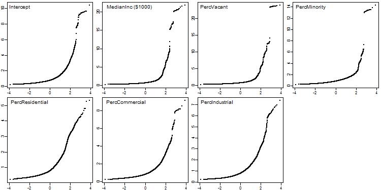
Figure 9: Permutation distributions of ${\boldsymbol{\hat{R\!A\!V}}_{\!\!j}}$ for the LA Homeless Data

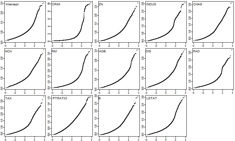
Figure 10: Permutation distributions of ${\boldsymbol{\hat{R\!A\!V}}_{\!\!j}}$ for the Boston Housing Data

References

- [1] Aldrich, J. (2005). Fisher and Regression. Statistical Science 20 (4), 4001–417.
- [2] Berk, R., Brown, L., Buja, A., Zhang, K., and Zhao, L. (2013). Valid Post-Selection Inference. The Annals of Statistics 41 (2), 802–837.
- [3] Berk, R. H. (1966). Limiting Behavior of Posterior Distributions When the Model is Incorrect. The Annals of Mathematical Statistics 37 (1), 51–58.
- [4] Berk, R. H. (1970). Consistency A Posteriori. The Annals of Mathematical Statistics 41 (3), 894–960.
- [5] Berk, R. and Kriegler, B. and Yilvisaker, D. (2008). Counting the Homeless in Los Angeles County. in Probability and Statistics: Essays in Honor of David A. Freedman, Monograph Series for the Institute of Mathematical Statistics, D. Nolan and S. Speed (eds.)
- [6] Berman, M. (1988). A Theorem of Jacobi and its Generalization. Biometrika 75 (4), 779–783.
- [7] Bickel, P. J. and Götze, F. and van Zwet, W. R. (1997). Resampling Fewer than Observations: Gains, Losses, and Remedies for Losses. Statistica Sinica 7, 1–31.
- [8] Box, G. E. P. (1979). Robustness in the Strategy of Scientific Model Building. in Robustness in Statistics: Proceedings of a Workshop (Launer, R. L., and Wilkinson, G. N., eds.) Amsterdam: Academic Press (Elsevier), 201–236.
- [9] Bühlmann, P. and van de Geer, S. (2015). High-dimensional Inference in Misspecified Linear Models. arXiv:1503.06426
- [10] Buja, A. and Berk, R. and Brown, L. and George, E. and Kuchibhotla, A. K. Zhao, L. (2018). Models as Approximations: A General Theory of Model-Robust Regression. arXiv:1612.03257
- [11] Cox, D. R. and Hinkley, D. V. (1974). Theoretical Statistics, London: Chapman & Hall.
- [12] Cox, D.R. (1995). Discussion of Chatfield (1995). Journal of the Royal Statistical Society, Series A 158 (3), 455-456.
- [13] Davies, P. L. (2014). Data Analysis and Approximate Models. Boca Raton, FL: CRC Press.
- [14] De Blasi, P. (2013). Discussion of Walker (2013). Journal of Statistical Planning and Inference 143, 1634–1637.
- [15] Diggle, P. J. and Heagerty, P. and Liang, K.Y., and Zeger, S. L. (2002). Analysis of Longitudinal Data. Oxford Statistical Science Series. Oxford: Oxford University Press. ISBN 978-0-19-852484-7.
- [16] Donoho, D. D. and Montanari, A. (2014). Variance Breakdown of Huber (M)-estimators: . arXiv:1503.02106
- [17] Efron, B. (1982). The Jackknife, the Bootstrap and other Resampling Plans. Philadelphia, PA: Society for Industrial and Applied Mathematics (SIAM).
- [18] Efron, B. and Tibshirani, R. J. (1994). An Introduction to the Bootstrap, Boca Raton, FL: CRC Press.
- [19] Eicker, F. (1963). Asymptotic Normality and Consistency of the Least Squares Estimators for Families of Linear Regressions. The Annals of Mathematical Statistics 34 (2), 447-456.
- [20] El Karoui, N. and Bean, D. and Bickel, P. and Yu, B. (2013). Optimal M-Estimation in High-Dimensional Regression. Proceedings of National Academy of Sciences 110 (36), 14563-–14568.
- [21] Freedman, D. A. (1981). Bootstrapping Regression Models. The Annals of Statistics 9 (6), 1218–1228.
- [22] Freedman, D. A. (2006). On the So-Called “Huber Sandwich Estimator” and “Robust Standard Errors.” The American Statistician 60 (4), 299–302.
- [23] Gelman, A. and Park, D.. K. (2008). Splitting a Regressor at the Upper Quarter or Third and the Lower Quarter or Third, The American Statistician 62 (4), 1–8.
- [24] Hall, A. R. (2005). Generalized Method of Moments (Advanced Texts in Econometrics). Oxford: Oxford University Press. ISBN 0-19-877520-2.
- [25] Hall, P. (1992). The Bootstrap and Edgeworth Expansion. (Springer Series in Statistics) New York, NY: Springer Verlag.
- [26] Hampel, F. R. and Ronchetti, E. M. and Rousseeuw, P. J. and Stahel, W. A. (1986). Robust Statistics: The Approach based on Influence Functions. New York, NY: Wiley.
- [27] Hansen, L. P. (1982). Large Sample Properties of Generalized Method of Moments Estimators. Econometrica 50 (4), 1029–1054.
- [28] Harrison, X. and Rubinfeld, X. (1978). Hedonic Prices and the Demand for Clean Air. Journal of Environmental Economics and Management 5, 81–102.
- [29] Hartigan J. A. (1983). Asymptotic Normality of Posterior Distributions. In: Bayes Theory, Chapter 11, Springer Series in Statistics. New York, NY: Springer.
- [30] Hausman, J. A. (1978). Specification Tests in Econometrics. Econometrica 46 (6), 1251-1271.
- [31] Hinkley, D. V. (1977). Jackknifing in Unbalanced Situations. Technometrics 19, 285–292.
- [32] Hoff, P. and Wakefield, J. (2013). Bayesian Sandwich Posteriors for Pseudo-True Parameters — Discussion of Walker (2013). Journal of Statistical Planning and Inference 143, 1638–1642.
- [33] Huber, P. J. (1967). The Behavior of Maximum Likelihood Estimation under Nonstandard Conditions. Proceedings of the Fifth Berkeley Symposium on Mathematical Statistics and Probability, Vol. 1, Berkeley: University of California Press, 221–233.
- [34] Huber, P. J. and Ronchetti, E.M. (2009). Robust Statistics., 2nd ed. New York, NY: Wiley.
- [35] Kauermann, G. and Carroll, R. J. (2001). A Note on the Efficiency of Sandwich Covariance Matrix Estimation, Journal of the American Statistical Association 96(456), 1387-–1396.
- [36] Krasker, W. S. and Welsch, R. W. (1982). Efficient Bounded-Influence Regression Estimation. Journal of the American Statistical Association 77 (379), 595-604.
- [37] Lehmann, E. L. and Romano, J. P. (2008). Testing Statistical Hypotheses. New York, NY: Springer Verlag.
- [38] Liang, K.-Y. and Zeger, S. L. (1986). Longitudinal Data Analysis Using Generalized Linear Models. Biometrika 73 (1), 13-22.
- [39] Loh, P. (2015). Statistical Consistency and Asymptotic Normality for High-Dimensional Robust M-Estimators. arXiv:1501.00312
- [40] Long, J. S. and Ervin, L. H. (2000). Using Heteroscedasticity Consistent Standard Errors in the Linear Model. The American Statistician 54(3), 217-224.
- [41] MacKinnon, J. and White, H. (1985). Some Heteroskedasticity-Consistent Covariance Matrix Estimators with Improved Finite Sample Properties. Journal of Econometrics 29, 305–325.
- [42] Mammen, E. (1993). Bootstrap and Wild Bootstrap for High Dimensional Linear Models. The Annals of Statistics 21 (1), 255–285.
- [43] Mammen, E. (1996). Empirical process of residuals for high-dimensional linear models The Annals of Statistics 24 (1), 307-335.
- [44] McCarthy, D. and Zhang, K. and Berk, R. and Brown, L. and Buja, A. and George, E. and Zhao, L. (2016). Calibrated Percentile Double Bootstrap For Robust Linear Regression Inference. http://arxiv.org/abs/1511.00273
- [45] Newey, W. K. and West, K. D. (1987). A Simple, Positive Semi-definite, Heteroskedasticity and Autocorrelation Consistent Covariance Matrix. Econometrica 55 (3), 703-–708.
- [46] O’Hagan, A. (2013). Bayesian Inference with Misspecified Models: Inference about what? Journal of Statistical Planning and Inference 143, 1643–1648.
- [47] Owen, A. B. (2001). Empirical Likelihood. New York: Chapman & Hall/CRC Monographs on Statistics & Applied Probability.
- [48] Politis, D. N. and Romano, J. P. (1994). A General Theory for Large Sample Confidence Regions based on Subsamples under Minimal Assumptions. The Annals of Statistics 22, 2031–2050.
- [49] R Development Core Team (2008). R: A Language and Environment for Statistical Computing. R Foundation for Statistical Computing, Vienna, Austria. ISBN 3-900051-07-0, URL http://www.R-project.org.
- [50] Stigler, S. M. (2001). Ancillary History. In State of the Art in Probability and Statistics: Festschrift for W. R. van Zwet (M. DeGunst, C. Klaassen and A. van der Vaart, eds.), 555–567.
- [51] Szpiro, A. A. and Rice, K. M. and Lumley, T. (2010). Model-Robust Regression and a Bayesian “Sandwich” Estimator. The Annals of Applied Statistics 4 (4), 2099–-2113.
- [52] Lee, J. D. and Sun, D. L. and Sun, Y. and Taylor, J. E. (2016). Exact Post-Selection Inference, with Application to the Lasso. The Annals of Statistics 44 (3), 907–927.
- [53] Walker, S. G. (2013). Bayesian Inference with Misspecified Models. Journal of Statistical Planning and Inference 143, 1621–1633.
- [54] Wasserman, L. (2011). Low Assumptions, High Dimensions. Rationality, Markets and Morals (RMM) 2 (11), 201–209 (www.rmm-journal.de).
- [55] Weber, N.C. (1986). The Jackknife and Heteroskedasticity (Consistent Variance Estimation for Regression Models). Economics Letters 20, 161-–163.
- [56] White, H. (1980a). Using Least Squares to Approximate Unknown Regression Functions. International Economic Review 21 (1), 149-–170.
- [57] White, H. (1980b). A Heteroskedasticity-Consistent Covariance Matrix Estimator and a Direct Test for Heteroskedasticity. Econometrica 48, 817-–838.
- [58] White, H. (1981). Consequences and Detection of Misspecified Nonlinear Regression Models. Journal of the American Statistical Association 76 (374), 419-–433.
- [59] White, H. (1982). Maximum Likelihood Estimation of Misspecified Models. Econometrica 50, 1–25.
- [60] White, H. (1994). Estimation, Inference and Specification Analysis. Econometric Society Monographs No. 22. Cambridge, GB: Cambridge University Press.
- [61] Wu, C. F. J. (1986). Jackknife, Bootstrap and Other Resampling Methods in Regression Analysis. The Annals of Statistics 14 (4), 1261–1295.