Fast shuttling of a trapped ion in the presence of noise

Abstract

We theoretically investigate the motional excitation of a single ion caused by spring-constant and position fluctuations of a harmonic trap during trap shuttling processes. A detailed study of the sensitivity on noise for several transport protocols and noise spectra is provided. The effect of slow spring-constant drifts is also analyzed. Trap trajectories that minimize the excitation are designed combining invariant-based inverse engineering, perturbation theory, and optimal control.

I Introduction

A quantum information processing architecture based on shuttling individual or small groups of ions among different storing or processing sites requires fast transporting techniques that avoid decoherence and excitations at the arrival zone Wineland2002 ; Rowe ; Wineland2006 . A promising research and technological avenue Roos ; Monroe has been opened by recent experiments Rowe ; Home ; transna that demonstrate the feasibility of a transport-based architecture, even beyond (faster than) the adiabatic regime Bowler ; Schmidt . Such experiments on transport and fast splitting of ion crystals have been performed with optimized time-dependent control voltages and the outcome is analysed with spectroscopy precise at the level of single motional quanta Bowler ; Schmidt . A fundamental limit to the shuttling speed which can be achieved at a desired final excitation is given by the unavoidable presence of noise. Electric field noise in Paul traps has been characterized experimentally in Ref. TURCHETTE2000 by monitoring the heating out of the motional ground state. It was found that the corresponding noise level exceeds the limit given by Johnson noise by several orders of magnitude, an effect that has been termed anomalous heating. In a resting trap, it has been shown Lamoreaux that the heating rate is determined by the noise power spectral density at the trap frequency. This does not necessarily hold for shuttling operations, where a broader part of the noise spectrum and slow drifts of the trap parameters can compromise the shuttling result producing undesired excitation.
On many ion trap experiments, the frequency dependence of the electric field noise spectral density $S(\Omega)$ has been investigated by measuring heating rates for varying trap frequencies, and commonly a polynomial scaling $S(\Omega)\propto\Omega^{-\alpha}$ is observed. While a wide range of exponents $\alpha$ between -1 and 6 have been reported Brownnutt , in many cases a behavior consistent with flicker noise $\alpha\approx 1$ is observed. This indicates that a variety of noise spectra can occur and that resonances of technical origin can play a role. Fast shuttling operations ultimately require rapidly changing voltage waveforms BAIG2013 ; BOWLER2013 , which strongly restricts the possibility to mitigate noise by filtering. This leads us to the conclusion that it is worthwhile to investigate the sensitivity of shuttling protocols for colored noise. We also consider drifts of trap parameters, which are slow on the timescales of the trap period and the durations of shuttling operations. These drifts can be characterized by monitoring the trap frequency over time. On a trap similar to the design used in Schmidt , we find long-time variations of the trap frequency of up to 5%. These variations can be caused by drift of the trap voltages, thermal expansion of the trap and charging of the trap itself.
Faster than adiabatic trap trajectories without final excitation may be designed using invariant-based inverse engineering Erik1 ; Erikcond ; transOCT ; 2ions ; Mainz2 . This technique produces families of trajectories as reviewed in Sec. II. It is possible to choose among them the ones that optimize some variable of interest, for example the time average of the transient energy or of the displacement between the trap center and the center of mass transOCT . In the field of internal state control this type of multiplicity has been used to design protocols that minimize the effects of noise noise1 ; noise2 , and we shall apply this idea to ion transport too. In Sec. III, we shall consider two basic types of noise that affect a moving harmonic trap: spring-constant fluctuations and position fluctuations around the ideal trajectory (trap shaking). A basic challenge in transport-protocol design is to mitigate or suppress noise or systematic errors and their effects on the final state fidelities. Our aim is to characterize and minimize noise effects by finding optimal transport trajectories and strategies.
We provide general results for the final excitation energy for different noise power spectra by using a perturbative master-equation approach. A detailed study of the three relevant cases of white noise (flat spectrum), brown noise (Ornstein-Ulhenbeck process with Lorentzian spectrum) and pink or flicker noise (1/frequency spectrum in a frequency range) is performed.

In Sec. IV, trajectories are found that minimize the effect of a systematic (constant, not random) spring constant error, and, finally, we discuss how our theoretical results may be implemented experimentally.

II Invariant-based inverse engineering method

The harmonic transport of one ion is described here by the effective 1D Hamiltonian

$$H_{0}(t)=\frac{\hat{p}^{2}}{2m}+\frac{1}{2}m\omega^{2}[\hat{q}-q_{0}(t)]^{2},$$ (1)

where $\hat{q}$ and $\hat{p}$ are the position and momentum operators, $\omega/(2\pi)$ is the frequency of the trap, and $q_{0}(t)$ its center. The corresponding quadratic-in-momentum Lewis-Riesenfeld invariant LR ; LL ; DL is given in this case (up to an arbitrary multiplicative constant) by Erik1

$$I(t)=\frac{1}{2m}(\hat{p}-m\dot{q}_{c})^{2}+\frac{1}{2}m\omega^{2}[\hat{q}-q_{c}(t)]^{2},$$ (2)

where the function $q_{c}(t)$ must satisfy the auxiliary equation

$$\ddot{q}_{c}+\omega^{2}(q_{c}-q_{0})=0$$ (3)

to guarantee the invariant condition

$$\frac{dI(t)}{dt}\equiv\frac{\partial I(t)}{\partial t}+\frac{1}{i\hbar}[I(t),H_{0}(t)]=0.$$ (4)

The expectation value of $I(t)$ remains constant for solutions of the time-dependent Schrödinger equation $i\hbar\partial_{t}\Psi(q,t)=H_{0}(t)\Psi(q,t)$. They can be expressed in terms of independent “transport modes” $\Psi_{n}(q,t)=e^{i\alpha_{n}}\psi_{n}(q,t)$ as $\Psi(q,t)=\sum_{n}c_{n}e^{i\alpha_{n}}\psi_{n}(q,t),$ where $n=0,1,...$; $c_{n}$ are time-independent coefficients; and $\psi_{n}(q,t)$ are the orthonormal eigenvectors of the invariant $I(t)$ satisfying $I(t)\psi_{n}(q,t)=\lambda_{n}\psi_{n}(q,t)$, with real time-independent $\lambda_{n}$. The Lewis-Riesenfeld phase is

$$\alpha_{n}(t)=\frac{1}{\hbar}\int_{0}^{t}\Big{\langle}\psi_{n}(t^{\prime})\Big{|}i\hbar\frac{\partial}{\partial t^{\prime}}-H_{0}(t^{\prime})\Big{|}\psi_{n}(t^{\prime})\Big{\rangle}dt^{\prime}.$$ (5)

For the harmonic trap considered here Erik1 ,

$$\psi_{n}(q,t)=\exp{\left(i\frac{m\dot{q}_{c}q}{\hbar}\right)}\psi_{n}^{0}(q-q_{c}),$$ (6)

where $\psi_{n}^{0}(q)$ are the eigenstates of Eq. (1) for $q_{0}(t)=0$. Note that $q_{c}$ is the center of mass of the transport modes obeying the classical Newton equation (3).

Suppose that the harmonic trap is displaced from $q_{0}(0)=0$ to $q_{0}(T)=d$ in a shuttling time $T$. The trajectory $q_{0}(t)$ of the trap can be inverse engineered by designing first an appropriate classical trajectory $q_{c}(t)$. To guarantee the commutativity of $I(t)$ and $H_{0}(t)$ at $t=0$ and $t=T$, which implies the mapping between initial and final trap eigenstates without final excitation, we set the conditions Erik1

$$q_{0}(0)=q_{c}(0)=0,~{}~{}\dot{q}_{c}(0)=0,$$

$$q_{0}(T)=q_{c}(T)=d,~{}~{}\dot{q}_{c}(T)=0.$$ (7)

The additional conditions

$$\ddot{q}_{c}(0)=0,~{}~{}\ddot{q}_{c}(T)=0$$ (8)

may be imposed to avoid sudden jumps in the trap position. However discontinuities of $\ddot{q}_{c}(t)$ may in general be allowed: they correspond to ideal instantaneous trap displacements inducing a sudden finite jump of the acceleration, whereas the velocity $\dot{q}_{c}$ and the trajectory $q_{c}$ remain continuous. In the following, we consider for simplicity the transport of the single mode $n$ in the noiseless limit ($n=0$ in the numerical examples), and examine the excitation energy of the system energy due to noise or errors, as well as ways to suppress or minimize it.

III Noise

To study the effect of the noise we follow the master equation treatment in diosi1 ; diosi2 ; strunzpla . The Hamiltonian is assumed to be of the form

$$H(t)=\frac{\hat{p}^{2}}{2m}+\frac{1}{2}m\omega^{2}[\hat{q}-q_{0}(t)]^{2}+Lx(t),$$ (9)

where $L$ is a system operator coupling to the environment. The fluctuating variable $x(t)$ satisfies

$${\cal{E}}[x(t)]=0,~{}~{}{\cal{E}}[x(t)x(s)]=\alpha(t-s),$$ (10)

where $\alpha(t-s)$ is the correlation function of the noise and $\cal{E}[...]$ the statistical expectation. The correlation function and the spectral power density are related by the Wiener-Khinchin theorem,

$$S(\Omega) = \frac{1}{2\pi}\int_{-\infty}^{\infty}\alpha(\tau)\cos(\Omega\tau)d\tau,$$ (11)

$$\alpha(\tau) = \int_{-\infty}^{\infty}S(\Omega)\cos(\Omega\tau)d\Omega.$$ (12)

By expanding in the ratio between environmental correlation time and the typical time scale of the system yuting , a closed master equation can be derived retaining first order corrections to the Markovian limit,

$$\frac{d}{dt}\rho=-\frac{i}{\hbar}[H_{0},\rho]+\frac{1}{\hbar}[L,\rho\bar{O}(t)^{{\dagger}}]-\frac{1}{\hbar}[L^{{\dagger}},\bar{O}(t)\rho],$$ (13)

where

$$\bar{O}(t)=\frac{1}{\hbar}g_{0}(t)L-\frac{i}{\hbar^{2}}g_{1}(t)[H_{0},L]-\frac{g_{2}(t)}{\hbar^{3}}[L^{{\dagger}},L]L,$$ (14)

and

$$g_{0}(t) = \int_{0}^{t}\alpha(t-s)ds,$$ (15)

$$g_{1}(t) = \int_{0}^{t}\alpha(t-s)(t-s)ds,$$ (16)

$$g_{2}(t) = \int_{0}^{t}\int_{0}^{s}\alpha(t-s)\alpha(s-u)(t-s)du\,ds.$$ (17)

We insist that the master equation (13) is valid on the condition that the noise correlation time is small compared to the typical system time scales, so that $g_{1}$ and $g_{2}$ terms must be corrections to the dominant $g_{0}$ term.

III.1 Spring constant noise

We consider now a fluctuating spring constant by setting $L=\frac{1}{2}m\omega^{2}(\hat{q}-q_{0})^{2}$. Then

$$\bar{O}(t)=\frac{m\omega^{2}}{2\hbar}(t)g_{0}(t)(\hat{q}-q_{0})^{2}+\frac{2}{m\hbar}g_{1}(t)\!\!\left[\hat{p}q_{0}-\frac{1}{2}(\hat{p}\hat{q}+\hat{q}\hat{p})\right]\!,$$ (18)

and the master equation (13) becomes

$$\frac{d}{dt}\rho= - \frac{i}{\hbar}[H_{0},\rho]-\frac{m^{2}\omega^{4}}{4\hbar^{2}}g_{0}(t)\left[(\hat{q}-q_{0})^{2},[(\hat{q}-q_{0})^{2},\rho]\right]$$ (19)

$$- \frac{m\omega^{4}}{2\hbar^{2}}g_{1}(t)\!\!\left[(\hat{q}-q_{0})^{2},[\hat{p}q_{0}-\frac{1}{2}(\hat{p}q+q\hat{p}),\rho]\right]\!.$$

Using time-dependent perturbation theory for the master equation we may write the density operator as (for an alternative non-perturbative approach see the Appendix A)

$$\rho(T) \simeq \rho_{0}(T)+\frac{m^{2}\omega^{4}}{4\hbar^{2}}\int_{0}^{T}g_{0}(t)\widetilde{U}_{0}(T,t)\widetilde{J}_{1}(t)\rho_{0}(t)dt$$ (20)

$$+ \frac{m\omega^{4}}{2\hbar^{2}}\int_{0}^{T}g_{1}(t)\widetilde{U}_{0}(T,t)\widetilde{J}_{2}(t)\rho_{0}(t)dt,$$

where the subscript $``0"$ represents noiseless unitary dynamics, $\rho_{0}(T)=|\Psi_{n}(T)\rangle\langle\Psi_{n}(T)|$, and $\widetilde{U}_{0}(T,t)$ is the noiseless evolution superoperator, i.e.,

$$\rho_{0}(t)=\widetilde{U}_{0}(t,t^{\prime})\rho_{0}(t^{\prime})=U_{0}(t,t^{\prime})\rho_{0}(t^{\prime})U_{0}^{{\dagger}}(t,t^{\prime}),$$ (21)

where $U_{0}(t,t^{\prime})$ is the noiseless evolution operator. $\widetilde{J}_{1}(t)$ and $\widetilde{J}_{2}(t)$ are superoperators,

$$\!\!\widetilde{J}_{1}(t)\rho_{0}(t)\! \!=\! \!-[(\hat{q}-q_{0})^{2}\!,\![(\hat{q}-q_{0})^{2},\rho_{0}(t)]],$$ (22)

$$\!\!\widetilde{J}_{2}(t)\rho_{0}(t) = \!-\!\bigg{[}\!(\hat{q}-q_{0})^{2}\!,\!\bigg{[}\hat{p}q_{0}\!-\!{{\frac{(\hat{p}\hat{q}+\hat{q}\hat{p})}{2}}},\rho_{0}(t)\!\bigg{]}\!\bigg{]}\!.$$ (23)

A detailed calculation gives the final energy corresponding in the noiseless limit to the $n_{th}$ mode,

$${\langle}H_{0}(T){\rangle}_{n} = tr[H_{0}(T)\rho(T)]\simeq{\langle}\Psi_{n}(T)|H_{0}(T)|\Psi_{n}(T){\rangle}$$

$$+ \frac{m^{2}\omega^{4}}{4\hbar^{2}}\int_{0}^{T}g_{0}(t){\langle}\Psi_{n}(t)|\widetilde{J}_{1}(t)H^{\prime}(t)|\Psi_{n}(t){\rangle}dt$$

$$+ \frac{m\omega^{4}}{2\hbar^{2}}\int_{0}^{T}g_{1}(t){\langle}\Psi_{n}(t)|\widetilde{J}_{3}(t)H^{\prime}(t)|\Psi_{n}(t){\rangle}dt$$

$$= E_{n}+\hbar\omega^{3}\left(n+\frac{1}{2}\right)\int_{0}^{T}g_{0}(t)dt,$$

$$+ m\int_{0}^{T}[g_{0}(t)\ddot{q}_{c}^{2}(t)+\omega^{2}g_{1}(t)\dot{q}_{c}(t)\ddot{q}_{c}(t)]dt,$$

where $E_{n}=(n+1/2)\hbar\omega$,

$$\widetilde{J}_{3}(t)H^{\prime}(t)=-\left[\hat{p}q_{0}-\frac{1}{2}(\hat{p}\hat{q}+\hat{q}\hat{p}),[(\hat{q}-q_{0})^{2},H^{\prime}(t)]\right],$$

and $H^{\prime}(t)=U_{0}^{{\dagger}}(T,t)H_{0}(T)U_{0}(T,t)$.

The following subsections deal with different noise types according to their spectrum. We pay much attention to white noise because our method is perturbative, so understanding this reference case in depth is fundamental. In addition, white noise is amenable of analytical treatment and explicit optimization of trap trajectories.

III.1.1 White noise

The correlation function for white noise is $\alpha(\tau)=\gamma\delta(\tau)$, and the corresponding power spectrum is constant, $S(\Omega)=\frac{\gamma}{2\pi}$. Here $\gamma$ scales the noise and

$$g_{0}(t)=\gamma/2,~{}g_{1}(t)=0.$$ (24)

The instantaneous energy in Eq. (III.1) can be expressed as

$${\langle}H_{0}(T){\rangle}_{n}=E_{n}+\gamma G(T),$$ (25)

where

$$G(T)=\frac{m}{2}\int_{0}^{T}\ddot{q}_{c}^{2}(t)dt+\frac{\hbar\omega^{3}}{2}\left(n+\frac{1}{2}\right)T.$$ (26)

The excitation energy is $E_{e}=\gamma G(T)$. The first term of $G(t)$ contains an integral of $\ddot{q}_{c}(t)$ and the mass of the ion, it reflects the fact that larger displacements from the trap center, see Eq. (3), increase the effect of spring constant fluctuations. The second term depends on trap frequency and the final time, and it is independent of the trajectory, so it can only be reduced by speeding up the transport. For fixed $T$, however, it is possible to design the trajectory $q_{c}(t)$ to make $G(T)$ as small as possible and minimize the integral. We shall now consider four different protocols. Examples of the corresponding trap trajectories $q_{0}(t)$ are provided in Fig. 1.

Polynomial protocol. A simple choice satisfying all boundary conditions and trap position continuity is a polynomial ansatz $q_{c}(t)=\sum_{n=0}^{5}\beta_{n}t^{n}$. The $\beta_{n}$ can be solved from the boundary conditions (II) and (8) to give

$$q_{c}(t)=d(10s^{3}-15s^{4}+6s^{5}),$$ (27)

where $s=t/T$, and the corresponding trap trajectory $q_{0}(t)$ is obtained from Eq. (3), see Fig. 1. $G(t)$ becomes

$$G(T)=\frac{60md^{2}}{7T^{3}}+\frac{(2n+1){\hbar\omega^{3}}}{4}T,$$ (28)

which is depicted in Fig. 2 (red dotted line). Short times are dominated by an inverse-cubic-in-time, frequency-independent term, and long times by a linear-in-time, $d$-independent term that accumulates the effect of noise. A minimum exists at $T=T_{min}=\sqrt[4]{\frac{720md^{2}}{7(2n+1)\hbar\omega^{3}}}$. For the realistic parameters of the figures, $T_{min}=73.2$ $T_{0}$, where $T_{0}=2\pi/\omega$ is the oscillation period. This $T_{min}$ is quite a large time (not shown in Fig. 2) well into the adiabatic regime.

Optimal control. To minimize $G(T)$ for a given $n$ and fixed transport time $T$, we may apply optimal control theory with the cost function

$$J_{E}=\int_{0}^{T}\ddot{q}_{c}^{2}(t)dt=\int^{T}_{0}\omega^{4}|q_{c}(t)-q_{0}(t)|^{2}dt,$$ (29)

subjected to the conditions (II), and a constrained (bounded) displacement $|q_{c}(t)-q_{0}(t)|\leq\delta$. This optimal-control problem was worked out in transOCT to minimize the time-average of the potential energy. Incidentally, this also minimizes the small effects of fast ion shuttling on the internal states due to the dc Stark shift phaseshift and adverse effects arising from anharmonicities of the trap potentials 2ions . The optimal $q_{c}(t)$ ($q_{0}(t)$ follows from Eq. (3), see Fig. 1) is transOCT

$$q_{c}(t)=\left\{\begin{array}[]{lll}0,&t\leq 0\\ \frac{1}{2}\omega^{2}t^{2}\delta,&0<t<t_{1}\\ -\frac{1}{6}\omega^{2}c_{1}(t-\frac{T}{2})^{3}+v_{0}t+c_{2},&t_{1}<t<t_{1}+t_{2}\\ d-\frac{1}{2}{\omega^{2}}(t-T)^{2}\delta,&t_{1}+t_{2}<t<T\\ d,&t\geq T\end{array}\right.,$$ (30)

where $c_{1}=\frac{2\delta}{T-2t_{1}},~{}v_{0}=\frac{1}{4}\omega^{2}\delta(T+2t_{1}),c_{2}=\frac{1}{2}(d-v_{0}T)$, and $t_{1}=\frac{T}{2}\left(1-\sqrt{3}\sqrt{1-\frac{4d}{\omega^{2}T^{2}\delta}}\right)$. $G(T)$ becomes

$$G(T)={\hbar\omega^{3}}\left[\frac{m\omega}{2\hbar}\bigg{(}2\delta^{2}t_{1}+\frac{c_{1}^{2}t_{2}^{3}}{12}\bigg{)}+\frac{2n+1}{4}T\right].$$ (31)

These equations hold for the time window

$$\sqrt{\frac{4d}{\omega^{2}\delta}}\leq T\leq\sqrt{\frac{6d}{\omega^{2}\delta}}.$$ (32)

For smaller times there is no solution to the “bounded control” optimization problem. For larger times, the solution coincides with the one for “unbounded control”,

$$q_{c}=d(3s^{2}-2s^{3}).$$

“Unbounded control” here means that the displacement is allowed to take any value, and this “unbounded” solution may be applied to an arbitrarily short time $T$ Erik1 ; transOCT ; phaseshift . The corresponding $G(T)$ is

$$G(T)=\frac{6md^{2}}{T^{3}}+\frac{(2n+1)\hbar\omega^{3}}{4}T,$$ (33)

similar in behavior to the polynomial ansatz, see Fig. 2 (blue dashed line). The minimum occurs at $T=\sqrt[4]{\frac{72md^{2}}{(2n+1)\hbar\omega^{3}}}$. For the parameters of the numerical examples, $T_{min}=66.9$ $T_{0}$, again well into the adiabatic regime. The solid lines in Fig. 2 depict $G(T)$ in Eq. (31) for two values of the constraint.

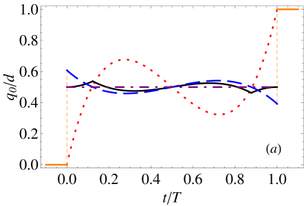
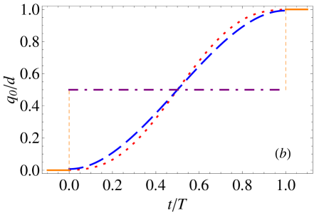
Figure 1: (Color online) Comparison of trap trajectories $q_{0}$ between the initial and final trap positions (yellow solid segments). Polynominal protocol (red dotted line); bounded optimal (black solid line, only in (a)); unbounded optimal (blue dashed line, the jump at the boundary times is $6d/(\omega^{2}T^{2})$); bang-bang (dot-dashed purple line). In (a) $T=T_{0}/2$ ($T_{0}$ is the oscillation period); in (b) $T=9T_{0}/2$. $\delta=0.5$ $d$, mass of ⁴⁰Ca⁺, initial state in $n=0$, $\omega=2\pi\times 1.4$ MHz, $d=280$ $\mu$m.

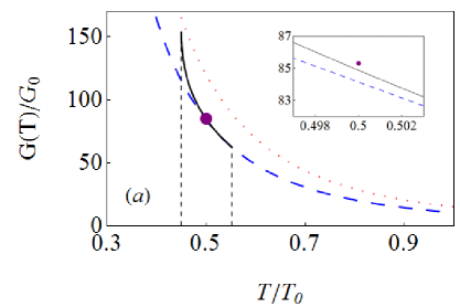
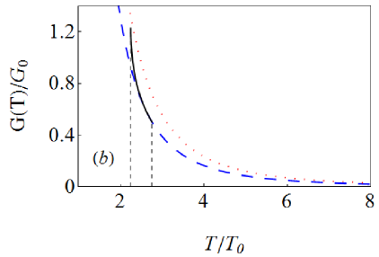
Figure 2: (Color online) G(T) versus final time. Polynominal ansatz (red dotted line), unbounded optimal (blue dashed line), bounded optimal (black solid line, the vertical dashed lines delimitate the time window in Eq. (32)), and bang-bang (purple dot, $T=T_{0}/2$, see the magnification in the inset). (a) $\delta=0.5\,d$, (b) $\delta=0.02\,d$, $G_{0}=\hbar\omega^{2}\times 10^{6}$, other parameters are the same as in Fig. 1.

Bang-bang protocol. Finally let us examine the simple bang-bang protocol Alonso

$$q_{0}(t)=\left\{\begin{array}[]{ll}0,&t\leq 0\hbox{},\\ d/2,&0<t<T\hbox{},\\ d,&t\geq T\hbox{}.\end{array}\right.$$ (37)

From Eq. (3), we can solve $q_{c}(t)$ as

$$q_{c}(t)=\frac{d}{2}-\frac{d}{2}\cos\omega t+\frac{d(1+\cos\omega T)}{2\sin\omega T}\sin\omega t.$$ (38)

To make $q_{c}(t)$ satisfy the boundary conditions (II), the final time must be an odd multiple of a semiperiod, $\omega T=(2k+1)\pi,~{}~{}k=0,1,2..$. Now

$$G(T)=\frac{m\omega^{4}d^{2}}{16}T+\frac{\hbar\omega^{3}(2n+1)}{4}T$$ (39)

increases linearly with time without a short-time inverse-cubic term characteristic of the previous protocols. For the minimal time, $T=T_{0}/2$, $G(T)$ is just slightly above that for the unbounded optimal, see the inset in Fig. 2 (a). $G(T)$ values for the next valid times ($3T_{0}/2$, $5T_{0}/2$…) are too high and out of scale in the figure. The unbounded optimal trajectory is quite close to the bang-bang one for $T=T_{0}/2$ but differs significantly from it for larger times, compare Figs. 1 (a) and 1 (b).

III.1.2 Ornstein-Uhlenbeck process

The Ornstein-Uhlenbeck (OU) noise is a natural generalization of the Markovian, white noise limit, with a finite correlation time $\tau$ and a power spectrum of Lorentzian form

$$S(\Omega)=\frac{D}{2\pi(1+\Omega^{2}\tau^{2})},$$ (40)

where $D$ is the noise intensity. When $\tau\rightarrow 0$, it reduces to white noise, and is also instrumental in generating flicker noise (see the following subsection) by superposing a range of correlation times. The correlation function corresponding to Eq. (40) is

$$\alpha(t)=\frac{D}{2\tau}e^{-t/\tau},$$ (41)

so that

$$g_{0}(t) = \frac{D}{2}(1-e^{-t/\tau}),$$ (42)

$$g_{1}(t) = \frac{D\tau}{2}\left(1-e^{-t/\tau}-\frac{t}{\tau}e^{-t/\tau}\right).$$ (43)

The energy in Eq. (III.1) will be

$${\langle}H_{0}(T){\rangle}_{n}=E_{n}+DG(T),$$

where the excitation energy is $E_{e}(T)=DG(T)$ and

$$G(T)=\frac{\hbar\omega^{3}}{4}\left(2n+1\right)\left(T-\tau+\tau e^{-T/\tau}\right)$$

$$+\frac{m}{2}\int_{0}^{T}\left[(1-e^{-t/\tau})\ddot{q}_{c}^{2}(t)-\frac{\omega^{2}t}{2\tau}e^{-t/\tau}\dot{q}_{c}^{2}(t)\right]dt.$$

In the small $\tau$ limit, integrating by parts and retaining only linear terms,

$$G(T) = \frac{\hbar\omega^{3}}{2}\left(n+\frac{1}{2}\right)\left(T-\tau\right)$$ (44)

$$+ \frac{m}{2}\left[\int_{0}^{T}\ddot{q}_{c}^{2}(t)dt-\tau\ddot{q}_{c}^{2}(0)\right].$$

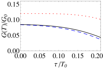
Figure 3: (Color online) G(T) for Ornstein-Uhlenbeck noise versus correlation time. Polynomial ansatz (red dotted line), unbounded optimal (blue dashed line), and bounded optimal (black solid line). $\delta=0.005\,d$, $T=5T_{0}$, $G_{0}=\hbar\omega^{2}\times 10^{6}$ and other parameters are the same as in Fig. 1.

The two correcting terms proportional to $\tau$ are negative so that the noise effect is reduced with respect to white noise. In Fig. 3 we plot $G(T)$ versus correlation time using the polynomial protocol and the protocols optimized for white noise.

III.1.3 Flicker noise

Flicker noise, with $\sim 1/\Omega$ spectrum in a range $\Omega_{2}<\Omega<\Omega_{1}$, may be modeled by summing over Lorentzian (Ohrnstein-Uhlenbeck) noises Hooge ; watanabe with proper statistical weights. Specifically we consider Hooge

$$\alpha(t)=\frac{C}{\ln(\tau_{2}/\tau_{1})}\int_{\tau_{1}}^{\tau_{2}}\frac{1}{\tau}e^{-t/\tau}d\tau,$$ (45)

where $C={\cal{E}}[x^{2}(t)]=\alpha(0)$. Using Eq. (11), the corresponding power spectrum takes the form

$$S(\Omega) = \frac{C}{\pi\ln(\tau_{2}/\tau_{1})}\int_{\tau_{1}}^{\tau_{2}}\frac{d\tau}{1+\Omega^{2}\tau^{2}}$$ (49)

$$= \left\{\begin{array}[]{ll}\frac{C(\tau_{2}-\tau_{1})}{\pi\ln(\tau_{2}/\tau_{1})},&\hbox{}\Omega\ll\Omega_{2},\\ \frac{C}{2\ln(\tau_{2}/\tau_{1})}\frac{1}{\Omega},&\hbox{}\Omega_{2}\ll\Omega\ll\Omega_{1},\\ \frac{C(\tau_{2}-\tau_{1})}{\pi\ln(\tau_{2}/\tau_{1})}\frac{1}{\tau_{1}\tau_{2}\Omega^{2}},&\hbox{}\Omega\gg\Omega_{1}.\end{array}\right.$$

where $\Omega_{1,2}=(2\pi)/\tau_{1,2}$. The spectrum is white if the frequency is below $\Omega_{2}$ and decays as $1/\Omega^{2}$ above $\Omega_{1}$. Eq. (45) leads to

$$g_{0}(t) = \frac{C}{\ln(\tau_{2}/\tau_{1})}\left[\tau-\tau e^{-t/\tau}-tEi\left(\frac{-t}{\tau}\right)\right]_{\tau_{1}}^{\tau_{2}},$$ (50)

$$g_{1}(t) = \frac{C}{2\ln(\tau_{2}/\tau_{1})}$$ (51)

$$\times \!\left[\tau^{2}(1\!-\!e^{t/\tau})\!-\!t\tau e^{-t/\tau}\!-\!t^{2}Ei\left(\frac{-t}{\tau}\right)\right]_{\tau_{1}}^{\tau_{2}}\!\!.$$

Here $Ei[-x]=\int_{-\infty}^{-x}(e^{t}/t)dt$ with $x>0$, which behaves as $Ei[-x]\simeq-e^{-x}/x$ for $x\rightarrow\infty$, and $Ei[-x]\simeq\gamma_{E}+\ln x$ for $x\rightarrow 0$, where $\gamma_{E}$ is Euler’s constant. The energy (III.1) takes the form

$${\langle}H_{0}(T){\rangle}_{n}=E_{n}+\frac{2C(\tau_{2}-\tau_{1})}{\ln(\tau_{2}/\tau_{1})}G(T),$$ (52)

where the excitation energy is $E_{e}(T)=\frac{2C(\tau_{2}-\tau_{1})}{\ln(\tau_{2}/\tau_{1})}G(T)$ and

$$G(T)=\frac{\hbar\omega^{3}}{4(\tau_{2}-\tau_{1})}\left(n+\frac{1}{2}\right)\left[\tau T(2-e^{-T/\tau})+\tau^{2}(e^{-T/\tau}-1)-T^{2}Ei\bigg{(}\!\!\!-\frac{T}{\tau}\bigg{)}\right]_{\tau_{1}}^{\tau_{2}}$$

$$+\frac{m}{2(\tau_{2}-\tau_{1})}\int_{0}^{T}\left\{\ddot{q}_{c}^{2}(t)\left[\tau-\tau e^{-t/\tau}-tEi\bigg{(}\!\!\!-\frac{t}{\tau}\bigg{)}\right]_{\tau_{1}}^{\tau_{2}}+\frac{\omega^{2}t}{2}\dot{q}_{c}^{2}(t)Ei\bigg{(}\!\!\!-\frac{t}{\tau}\bigg{)}\bigg{|}_{\tau_{1}}^{\tau_{2}}\right\}dt.$$ (53)

For $\tau_{2}/T\ll 1$ and $\dot{q_{c}}(0)=0$, we find, integrating by parts, the approximation

$$G(T) \simeq \frac{\hbar\omega^{3}}{2}\left(n+\frac{1}{2}\right)\left(T-\frac{\tau_{2}+\tau_{1}}{2}\right)$$ (54)

$$+ \frac{m}{2}\left[\int_{0}^{T}\ddot{q}_{c}^{2}(t)dt-\frac{\tau_{2}+\tau_{1}}{2}\ddot{q}_{c}^{2}(0)\right],$$

with a small correction to the white noise case similar to the one found for Ornstein-Uhlenbeck noise. Fig. 4 depicts $G(T)$ versus $\tau_{2}$ for the polynomial protocol and the protocols optimized in the Markovian limit.

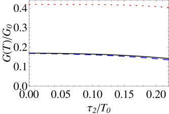
Figure 4: (Color online) $G(T)$ for flicker noise versus upper limit of the interval of correlation times $\tau_{2}$. Polynomial ansatz (red dotted line), unbounded optimal (blue dashed line), and bounded optimal (black solid line). $\delta=0.5\,d$, $G_{0}=\hbar\omega^{2}\times 10^{6}$, $\tau_{1}=1\times 10^{-10}$ $s$, $T=5T_{0}$, and other parameters are the same as in Fig. 1.

III.2 Position noise

In this subsection we define $L=K(\hat{q}-q_{0})$ in Eqs. (9) and (13) to simulate the effect of the environment on a fluctuating trap position. The master equation (13) takes the form

$$\frac{d}{dt}\rho= - \frac{i}{\hbar}[H_{0},\rho]-\frac{K^{2}}{\hbar^{2}}g_{0}(t)\left[\hat{q}-q_{0},[\hat{q}-q_{0},\rho]\right]$$ (55)

$$+ \frac{K^{2}}{m\hbar^{2}}g_{1}(t)\left[\hat{q}-q_{0},[\hat{p},\rho]\right].$$

Using the same time-dependent perturbation theory approach as in the previous section, the density matrix is

$$\rho(T) \simeq \rho_{0}(T)+\frac{K^{2}}{\hbar^{2}}\int_{0}^{T}g_{0}(t)\widetilde{U}_{0}(T,t)\widetilde{J}_{2}(t)\rho_{0}(t)dt$$

$$+ \frac{K^{2}}{m\hbar^{2}}\int_{0}^{T}g_{1}(t)\widetilde{U}_{0}(T,t)[\hat{q},[\hat{p},\rho_{0}(t)]]dt,$$

where the system energy is

$${\langle}H_{0}(T){\rangle}_{n} = tr[H_{0}(T)\rho(T)]\simeq{\langle}\Psi_{n}(T)|H_{0}(T)|\Psi_{n}(T){\rangle}$$ (56)

$$+ \frac{K^{2}}{\hbar^{2}}\!\!\int_{0}^{T}\!\!\!g_{0}(t){\langle}\Psi_{n}(t)|\widetilde{J}_{2}(t)H^{\prime}(t)|\Psi_{n}(t){\rangle}dt$$

$$+ \frac{K^{2}}{m\hbar^{2}}\!\!\int_{0}^{T}\!\!\!g_{1}(t){\langle}\Psi_{n}(t)|[\hat{p},[\hat{q},H^{\prime}(t)]]|\Psi_{n}(t){\rangle}dt$$

$$= E_{n}+\frac{K^{2}}{m}\int_{0}^{T}g_{0}(t)dt.$$

The excitation energy at the final time is independent of the trap trajectory, and depends only on the transport time. The only strategy left to minimize the effect of position fluctuations is to speed up the transport making $T$ as small as possible. The independence on the trajectory may be understood already at classical level from the solution of Eq. (3), $q_{c}(t)=q_{0}(t)-\int_{0}^{t}dt^{\prime}\dot{q}_{0}(t^{\prime})\cos[\omega(t-t^{\prime})]$. Note that a deviation from $q_{c}(t)$ due to a modified trajectory $q_{0}+\delta q_{0}$ depends only on $\delta q_{0}$ and its time derivative, not on $q_{0}$ itself. As a consequence, studies of excitation or heating rates for non-shuttling traps are directly applicable Savard1 ; Savard2 ; Milburn ; Lamoreaux .

IV Systematic spring constant error

Assume that the trap trajectory is designed for a given spring constant $\omega^{2}$, but the actual one is different, $\omega^{2}(1+\lambda)$. $\lambda$ may change from run to run but remain constant throughout the transport time. This is quite common as a consequence of experimental drifts and imperfect calibration. In current experiments it is likely to dominate other imperfections. Our objective here is to determine the induced excitation and to find trap trajectories that minimize the excitation in a range of $\lambda$ around 0. The system Hamiltonian is

$$H(t)=\frac{\hat{p}^{2}}{2m}+\frac{1}{2}m\omega^{2}(1+\lambda)[\hat{q}-q_{0}(t)]^{2},$$ (57)

where $\lambda$ is the relative error in the spring constant. For the actual frequency, the auxiliary equation is

$$\ddot{Q}_{c1}(t)+\omega_{1}^{2}(Q_{c1}-q_{0})=0,$$ (58)

with $\omega_{1}^{2}=\omega^{2}(1+\lambda)$. We define $Q_{c1}(t)=q_{c}(t)+f(t)$. Combining Eqs. (3) and (58), $f(t)$ satisfies

$$\ddot{f}(t)+\omega^{2}_{1}f(t)=\lambda\ddot{q}_{c}(t),$$ (59)

which is solved by

$$f(t) = \frac{\lambda}{\omega_{1}}\sin(\omega_{1}t)\int_{0}^{t}\ddot{q}_{c}(t^{\prime})\cos(\omega_{1}t^{\prime})dt^{\prime}$$ (60)

$$- \frac{\lambda}{\omega_{1}}\cos(\omega_{1}t)\int_{0}^{t}\ddot{q}_{c}(t^{\prime})\sin(\omega_{1}t^{\prime})dt^{\prime}.$$

For the new frequency $\omega_{1}$ and trajectory $Q_{c1}$, the exact energy of the system takes the form

$${\langle}H(T){\rangle}_{n} = \left(n+\frac{1}{2}\right)\hbar\omega_{1}+E_{e}(T),$$ (61)

where $E_{e}$ is the excitation energy,

$$E_{e}(T) = \frac{m\lambda^{2}}{2}\left[\int_{0}^{T}\ddot{q}_{c}(t)\cos(\omega_{1}t)dt\right]^{2}$$ (62)

$$+ \frac{m\lambda^{2}}{2}\left[\int_{0}^{T}\ddot{q}_{c}(t)\sin(\omega_{1}t)dt\right]^{2}.$$

To suppress the excitation energy, the trajectory $q_{c}(t)$ has to satisfy the conditions

$$\int_{0}^{T}\ddot{q}_{c}(t)\cos(\omega_{1}t)dt=0,~{}~{}~{}\int_{0}^{T}\ddot{q}_{c}(t)\sin(\omega_{1}t)dt=0.$$ (63)

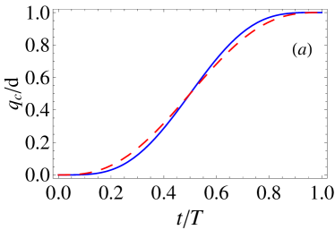
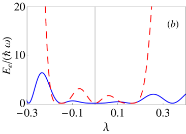
Figure 5: (Color online) (a) $q_{c}(t)$ versus $t$; (b) excitation energy versus $\lambda$. Dashed red line: quintic polynomial (27); solid blue line: seventh order polynomial in Eq. (64). $T=6.5\,T_{0}$ and other parameters are the same as in Fig. 1.

We approximate $\cos(\omega_{1}t)\simeq\cos(\omega t)$ and $\sin(\omega_{1}t)\simeq\sin(\omega t)$ to keep only quadratic terms in $\lambda$ in Eq. (62), and assume for $q_{c}$ a seventh order polynomial

$$q_{c}(t)=\sum_{n=0}^{7}c_{n}t^{n}$$ (64)

to satisfy the six conditions in Eqs. (II), (8) and

$$\int_{0}^{T}\ddot{q}_{c}(t)\cos(\omega t)\,dt=0,~{}~{}~{}\int_{0}^{T}\ddot{q}_{c}(t)\sin(\omega t)\,dt=0.$$ (65)

Doing the integrals formally, in terms of the unknown coefficients, we end up with a system of eight equations with eight unknowns (the $c_{n}$), which can be solved, but the expressions for the $c_{n}$ are too lengthy to be displayed here. The corresponding $q_{0}$ is obtained from Eq. (3). In Fig. 5 we have plotted the seventh order $q_{c}$ in Eq. (64) and the simplest quintic polynomial ansatz (27), as well as the corresponding excitation energies. The protocol based on Eq. (64) is more robust, i.e., it leads to smaller excitations when the actual trap frequency does not have the expected value. Alternative robustification schemes are possible adapted to specific needs, for example, imposing zero or minimal excitation at a discrete number of values of $\lambda$ in a given interval, see e.g. oldPRL for a similar approach applied to maximize the absorption of complex potentials.

Time-scaling errors are shown to be equivalent to spring-constant systematic errors in Appendix B, so the same strategies used here may be used in that case.

V Discussion

In this paper we have examined the excitation energy due to spring-constant noise/error and position noise in ions transported by a moving harmonic trap. We consider families of trajectories without final excitation in the noiseless limit and select optimal trap trajectories that minimize heating when the noise applies. For fixed shuttling time $T$, this selection is only possible for spring-constant noise/error, since for position noise the final energy increases linearly with $T$ but does not depend on any other feature of the trap trajectory.

We find an additional beneficial feature of the trajectories that minimize the effect of spring-constant noise even in the case that position noise is dominant: These trajectories minimize the time-average of the potential energy Erik1 ; transOCT , thus adverse effects of anharmonicity Mainz1 ; 2ions are suppressed.

Apart from trap trajectories with sudden, finite position jumps (optimal trap trajectories unconstrained or constrained by a maximum ion displacement with respect to the center of the trap, and simple bang-bang trajectories) we have as well considered smooth polynomial trajectories. For very short shuttling times (half an oscillation period) optimal control and bang-bang solutions display a reduced noise sensitivity, although they imply the technical challenge of implementing sudden trap jumps. At moderate times and beyond (five oscillations or more) the bang-bang approach produces too much excitation and the polynomial behaves similarly to the optimal trajectory.

Advances in the fabrication of micro structured ion traps and fast control electronics have allowed to experimentally reach the limits of adiabacity, thus the proposed protocols may be tested and the respective noise-sensitivity verified. Envisaged experiments at shuttle times of the order of an oscillation period Alonso require changes of the trapping potential on timescales much shorter than the period corresponding to the trap frequency. At such fast temporal changes of the control voltages, the cut-off frequency for noise filtering elements must be very high, and thus we expect that it might be increasingly difficult to reach a low noise level. As additionally the noise sensitivity of the shuttling results is increasing at fast timescales, the importance of noise-suppression by trajectory design becomes obvious. In the well-controlled setting of an ion trap, one may experimentally investigate the schemes with artificial injected designed noise arti1 ; arti2 . It is in experimental reach to design the spectral properties of a noise source and verify the predicted effects. The accuracy of sideband spectroscopy to determine the excess energy has reached sub-phonon level, such that even small optimization effects would be visible.

Acknowledgments— This work was supported by the Grants No. 61176118, 12QH1400800, 13PJ1403000, 2013310811003, IT472-10, FIS2009-12773-C02-01, UFI 11/55, and the Program for Professor of Special Appointment (Eastern Scholar) at Shanghai Institutions of Higher Learning. This research was also funded by the Office of the Director of National Intelligence (ODNI), Intelligence Advanced Research Projects Activity (IARPA), through the Army Research Office grant W911NF-10-1-0284. All statements of fact, opinion or conclusions contained herein are those of the authors and should not be construed as representing the official views or policies of IARPA, the ODNI, or the US Government.

Appendix A Closed equations for the moments

The quadratic and linear operators involving position and momentum form a dynamical Lie algebra (the Hamiltonian is a member of this algebra) for the Hamiltonians that describe spring constant noise and position noise. This leads to closed equations for the corresponding moments Milburn , which is interesting numerically, as the results are not perturbative in noise intensity. Also, physical consequences follow without even solving the system as we shall see.

For spring constant noise, the expectation values of position and momentum operators and their quadratic combinations satisfy, using Eq. (19),

$$\frac{d}{dt}\!\left(\!\!\begin{array}[]{c}{\langle}\hat{q}^{2}{\rangle}\\ {\langle}\hat{p}^{2}{\rangle}\\ {\langle}\hat{q}\hat{p}+\hat{p}\hat{q}{\rangle}\\ {\langle}\hat{q}{\rangle}\\ {\langle}\hat{p}{\rangle}\\ \end{array}\!\!\right)=M_{S}\left(\!\!\begin{array}[]{c}{\langle}\hat{q}^{2}{\rangle}\\ {\langle}\hat{p}^{2}{\rangle}\\ {\langle}\hat{q}\hat{p}+\hat{p}\hat{q}{\rangle}\\ {\langle}\hat{q}{\rangle}\\ {\langle}\hat{p}{\rangle}\\ \end{array}\!\!\right)+\left(\!\!\begin{array}[]{c}0\\ 8\hbar^{2}q_{0}^{2}g_{0}(t)\\ \frac{8\hbar^{2}}{m}q_{0}^{2}g_{1}(t)\\ 0\\ m\omega^{2}q_{0}-\frac{4\hbar^{2}}{m}q_{0}g_{1}(t)\\ \end{array}\!\!\right),$$ (66)

where

$$M_{S}=\left(\begin{array}[]{ccccc}0&0&\frac{1}{m}&0&0\\ 8\hbar^{2}g_{0}(t)&0&-m\omega^{2}&-16\hbar^{2}q_{0}g_{0}(t)&2m\omega^{2}q_{0}\\ -2m\omega^{2}+\frac{16\hbar^{2}}{m}g_{1}(t)&\frac{2}{m}&0&2m\omega^{2}q_{0}-\frac{8\hbar^{2}}{m}q_{0}g_{1}(t)&0\\ 0&0&0&0&\frac{1}{m}\\ 0&0&0&-m\omega^{2}+\frac{4\hbar^{2}}{m}g_{1}(t)&0\\ \end{array}\right).$$ (72)

For position noise, Eq. (55), the expectation values satisfy

$$\frac{d}{dt}\!\!\left(\!\!\!\begin{array}[]{c}{\langle}\hat{q}^{2}{\rangle}\\ {\langle}\hat{p}^{2}{\rangle}\\ {\langle}\hat{q}\hat{p}+\hat{p}\hat{q}{\rangle}\\ {\langle}\hat{q}{\rangle}\\ {\langle}\hat{p}{\rangle}\\ \end{array}\!\!\!\right)\!=\!M_{P}\!\left(\!\!\!\begin{array}[]{c}{\langle}\hat{q}^{2}{\rangle}\\ {\langle}\hat{p}^{2}{\rangle}\\ {\langle}\hat{q}\hat{p}+\hat{p}\hat{q}{\rangle}\\ {\langle}\hat{q}{\rangle}\\ {\langle}\hat{p}{\rangle}\\ \end{array}\!\!\!\right)\!\!+\!\!\left(\!\!\!\begin{array}[]{c}0\\ 2K^{2}g_{0}(t)\\ 2K^{2}g_{1}(t)/m\\ 0\\ m\omega^{2}q_{0}\\ \end{array}\!\!\!\right)$$ (89)

where

$$M_{P}=\left(\begin{array}[]{ccccc}0&0&1/m&0&0\\ 0&0&-m\omega^{2}&0&2m\omega^{2}q_{0}\\ -2m\omega^{2}&2/m&0&2m\omega^{2}q_{0}&0\\ 0&0&0&0&1/m\\ 0&0&0&-m\omega^{2}&0\\ \end{array}\right).$$ (90)

For colored or white position noise, the average position and momenta are not affected by the noise.

Appendix B Time scaling

We analyze here a systematic error in the clock used to design the trap trajectory so that instead of $q_{0}(t)$, the implemented trajectory is $q_{0}(\varepsilon t)$. The Hamiltonian is

$$H(t)=\frac{\hat{p}^{2}}{2m}+\frac{1}{2}m\omega^{2}[\hat{q}-q_{0}(\varepsilon t)],$$ (91)

and the Schrödinger equation $i\hbar\partial\Psi(t)/\partial t=H(t)\Psi(t)$ can be rewritten as

$$i\hbar\frac{\partial\Phi(\tau)}{\partial\tau}=H^{\prime}(\tau)\Phi(\tau),$$ (92)

where $\tau=\epsilon t$, $\Phi(\tau)=\Psi(t)$, and

$$H^{\prime}(\tau)=\frac{p^{2}}{2m^{\prime}}+\frac{1}{2}m^{\prime}\omega^{\prime 2}(\hat{q}-q_{0}(\tau)),$$ (93)

with $m^{\prime}=\varepsilon m$, and $\omega^{\prime}=\omega/\varepsilon$. Since $q_{0}(\tau)$ is designed for $\omega$, time scaling errors reduce formally to systematic spring-constant errors, and their effect can be suppressed or mitigated in the same manner.

References

- (1) D. Kielpinski, C. Monroe, and D. Wineland, Nature (London) 417, 709 (2002).
- (2) M.A. Rowe et al., Quantum Inf. Comput. 2, 257 (2002).
- (3) R. Reichle, D. Leibfried, R. B. Blakestad, J. Britton, J. D. Jost, E. Knill, C. Langer, R. Ozeri, S. Seidelin, and D. J. Wineland, Fortschr. Phys. 54, 666 (2006).
- (4) C. Roos, Physics 5, 94 (2012).
- (5) C. Monroe and J. Kim, Science 339, 1164 (2013).
- (6) J. P. Home, D. Hanneke, J. D. Jost, J. M. Amini, D. Leibfried, and D. J. Wineland, Science 325, 1227 (2009).
- (7) R. B. Blakestad, C. Ospelkaus, A. P. VanDevender, J. H. Wesenberg, M. J. Biercuk, D. Leibfried, and D. J. Wineland, Phys. Rev. A 84, 032314 (2011).
- (8) R. Bowler, J. Gaebler, Y. Lin, T. R. Tan, D. Hanneke, J. D. Jost, J. P. Home, D. Leibfried and D. J.Wineland, Phys. Rev. Lett. 109, 080502 (2012).
- (9) A. Walther, F. Ziesel, T. Ruster, S. T. Dawkins, K. Ott, M. Hettrich, K. Singer, F. Schmidt-Kaler, and U. Poschinger, Phys. Rev. Lett 109, 080501 (2012).
- (10) Q. A. Turchette, D. Kielpinski, B. E. King, D. Leibfried, D. M. Meekhof, C. J. Myatt, M. A. Rowe, C. A. Sackett, C. S. Wood, W. M. Itano, C. Monroe, and D. J. Wineland, Phys. Rev. A 61, 063418 (2000).
- (11) S. K. Lamoreaux, Phys. Rev. A 56, 4970 (1997).
- (12) M. Brownnutt et al., to be published.
- (13) M. T. Baig, M. Johanning, A. Wiese, S. Heidbrink, M. Ziolkowski, and C. Wunderlich, Rev. Sci. Instr. 84, 124701 (2013).
- (14) R. Bowler, U. Warring, J. W. Britton, B. C. Sawyer, and J. Amini, Rev. Sci. Instr. 84, 033108 (2013).
- (15) E. Torrontegui, S. Ibanez, X. Chen, A. Ruschhaupt, D. Guéry-Odelin and J. G. Muga, Phys. Rev. A 83, 013415 (2011).
- (16) E. Torrontegui, X. Chen, M. Modugno, S. Schmidt, A. Ruschhaupt, and J. G. Muga, New J. Phys. 14, 013031 (2012).
- (17) X. Chen, E. Torrontegui, D. Stefanatos, J.-S. Li, and J. G. Muga, Phys. Rev. A, 84, 043415 (2011).
- (18) M. Palmero, E. Torrontegui, D. Guéry-Odelin, and J. G. Muga, Phys. Rev. A 88, 053423 (2013).
- (19) H. A. Fürst, M. H. Goerz, U. G. Poschinger, M. Murphy, S. Montangero, T. Calarco, F. Schmidt-Kaler, K. Singer, C. P. Koch, arXiv: 1312.4156
- (20) A. Ruschhaupt, X. Chen, D. Alonso, and J. G. Muga, New J. Phys. 14, 093040 (2012).
- (21) X.-J. Lu, X. Chen, A. Ruschhaupt, D. Alonso, S. Guérin, and J. G. Muga, Phys. Rev. A 88, 033406 (2013).
- (22) H. R. Lewis and W. B. Riesenfeld, J. Math. Phys. 10, 1458 (1969).
- (23) H. R. Lewis and P. G. Leach, J. Math. Phys. 23, 2371 (1982).
- (24) A. K. Dhara and S. W. Lawande, J. Phys. A 17, 2324 (1984).
- (25) L. Diósi, Quantum Semiclassic. Opt. 8, 309 (1996).
- (26) L. Diósi and W. T. Strunz, Phys. Lett. A 235, 569 (1997).
- (27) W. T. Strunz, Phys. Lett. A 224, 25 (1996).
- (28) T. Yu, L. Diosi, N. Gisin, W. T. Strunz, Phys. Rev. A 60, 91 (1999).
- (29) Hoi-Kwan Lau, and Daniel F. V. James, Phys. Rev. A 83, 062330 (2011).
- (30) J. Alonso, F. M. Leupold, B. C. Keitch, and J. P. Home, New J. Phys. 15, 023001 (2013).
- (31) F. N. Hooge, P. A. Bobbert, Phys. B 239, 223 (1997).
- (32) S. Watanabe, Journal of the Korean Physical Society 46, 646 (2005).
- (33) T. A. Savard, K. M. O’Hara, and J. E. Thomas, Phys. Rev. A 56, R1095 (1997).
- (34) M. E. Gehm, K. M. O’Hara, T. A. Savard, and J. E. Thomas, Phys. Rev. A 58, 3914 (1998).
- (35) S. Schneider and G. J. Milburn, Phys. Rev. A 59, 3766 (1999).
- (36) J. P. Palao, J. G. Muga, and R. Sala, Phys. Rev. Lett. 80, 5469 (1998).
- (37) S. Schulz, U. Poschinger, K. Singer, and F. Schmidt- Kaler, Fortschr. Phys. 54, 648 (2006).
- (38) Q. A. Turchette, C. J. Myatt, B. E. King, C. A. Sackett, D. Kielpinski, W. M. Itano, C. Monroe, and D. J. Wineland, Phys. Rev. A 62, 053807 (2000).
- (39) C. J. Myatt, B. E. King, Q. A. Turchette, C. A. Sackett, D. Kielpinski, W. M. Itano, C. Monroe, and D.J. Wineland, Nature 403, 269 (2000).