Direct $N$-body simulations of globular clusters - II. Palomar 4

Abstract

We use direct $N$-body calculations to study the evolution of the unusually extended outer halo globular cluster Palomar 4 (Pal 4) over its entire lifetime in order to reproduce its observed mass, half-light radius, velocity dispersion and mass function slope at different radii.

We find that models evolving on circular orbits, and starting from a non-mass segregated, canonical initial mass function (IMF) can reproduce neither Pal 4 s overall mass function slope nor the observed amount of mass segregation. Including either primordial mass segregation or initially flattened IMFs does not reproduce the observed amount of mass segregation and mass function flattening simultaneously. Unresolved binaries cannot reconcile this discrepancy either. We find that only models with both a flattened IMF and primordial segregation are able to fit the observations. The initial (i.e. after gas expulsion) mass and half-mass radius of Pal 4 in this case are about 57000 M${\odot}$ and 10 pc, respectively. This configuration is more extended than most globular clusters we observe, showing that the conditions under which Pal 4 formed must have been significantly different from that of the majority of globular clusters. We discuss possible scenarios for such an unusual configuration of Pal 4 in its early years.

1 Introduction

Globular clusters are ideal astrophysical systems whose long-term evolution is determined by several internal and external processes, like mass loss due to stellar evolution and the energy-equipartition processes as well as tidal removal of star. In this regard, numerous numerical investigations have been carried out to understand their dynamical evolution (e.g. Giersz & Heggie 2011; see also the textbook by Heggie & Hut 2003). However, only within the last few years, with the introduction of graphics processing unit (GPU)-accelerated $N$-body codes such as nbody6 (Aarseth, 2003; Nitadori & Aarseth, 2012) it has become feasible to compute the dynamical evolution of massive star clusters over their entire lifetimes on a star-by-star basis. In Paper I of this series (Zonoozi et al., 2011), we presented the first direct $N$-body simulation of a Milky Way globular cluster over a Hubble time. For this project we chose the outer-halo globular cluster Palomar 14 (Pal 14), due to its relatively low mass and its large half-mass radius. In the paper, we presented a comprehensive set of $N$-body computations of Pal 14’s evolution over its entire lifetime and compared the results to the observed mass, half-light radius, flattened stellar mass function and velocity dispersion of Pal 14, which have been presented by Jordi et al. (2009). We showed that dynamical mass segregation alone cannot explain the mass function flattening in the cluster centre when starting from a canonical Kroupa initial mass function (IMF), and that a very high degree of primordial mass segregation would be necessary to explain this discrepancy. We concluded that such initial conditions for Pal 14 might be obtained by a violent early gas-expulsion phase from an embedded cluster born with mass segregation and a canonical IMF for low-mass stars, a thesis supported later by an independent study of an ensemble of globular clusters (Marks, Kroupa, & Baumgardt, 2008).

Here we aim at modelling the globular cluster Palomar 4 (Pal 4), which is similar to Pal 14 but has more complete observational data. Recently, Frank et al. (2012) presented an extensive observational study of Pal 4, revealing a flattened stellar mass function and significant mass segregation throughout the cluster. This additional knowledge of Pal 4 puts much stronger constraints on its current dynamical state.

Star clusters can undergo significant changes not only at birth but also during the course of their dynamical evolutions. It is therefore essential to specify to what extent the present-day properties of a globular cluster, e.g. their degree of mass segregation, are imprinted by early evolution and the formation processes, and to what extent they are the outcome of long-term dynamical evolution.

There are certain distinct mechanisms that can cause mass segregation. Dynamical mass segregation is the process by which the more massive stars of a gravitationally bound system sink towards the central regions, while lighter stars move further away from the centre. This process is a consequence of evolution towards energy equipartition driven by two-body encounters and is usually associated with the long-term evolution of clusters through the two-body relaxation process.

However, a number of observational studies (e.g. Hillenbrand 1997; Fischer et al. 1998; Hillenbrand & Hartmann 1998; de Grijs et al. 2002; Sirianni et al. 2002; Gouliermis et al. 2004; Stolte et al. 2006; Sabbi et al. 2008; Allison et al. 2009; Gouliermis, de Grijs, & Xin 2009) have found evidence of mass segregation in clusters with ages shorter than the time needed to produce the observed segregation via two-body relaxation (see also de Grijs 2010).

It has been suggested that the observed mass segregation in young clusters could be primordial – imprinted by the early star-formation process (Bonnell et al., 1997, 2001; Bonnell & Davies, 1998; Klessen, 2001; Bonnell & Bate, 2006). Such mass segregation could be due to the higher accretion rate of proto-stars in high-density regions of molecular clouds fragmenting into clumps. If individual clumps are mass segregated, it has been shown by McMillan, Vesperini, & Portegies Zwart (2007), that such primordial mass segregation would not be erased in the violent-relaxation phase during which clumps merge. The final system would preserve the mass segregation of the original clumps (see also Fellhauer, Wilkinson, & Kroupa 2009; Moeckel & Bonnell 2009). But even if such clumps are not initially segregated, the internal segregation time-scale can be shorter than the time needed for the clumps to merge. Hence, they will segregate internally via two-body relaxation and preserve this segregation after they have merged (McMillan, Vesperini, & Portegies Zwart 2007).

Alternatively, Bastian et al. (2008) found observational evidence for a strong expansion in the first 20 Myr of the evolution of six young M51 clusters and pointed out that this expansion could also lead to a rapid variation in the cluster relaxation time, thus, using the present-day relaxation time might lead to an underestimation of the possible role played by two-body relaxation in generating mass segregation in the early phases of a cluster’s dynamical evolution.

Regardless of the mechanism producing mass segregation, the presence of primordial (or early) mass segregation significantly affects the global dynamical evolution of star clusters (Gürkan, Freitag, & Rasio 2004; Baumgardt, De Marchi, & Kroupa 2008). For example, the early mass loss due to stellar evolution of high-mass stars has a stronger impact on initially segregated clusters than on unsegregated clusters (Vesperini et al. 2009). The degree of primordial or early mass segregation is therefore a crucial parameter in the modelling of globular clusters.

Another important quantity that has to be taken into account in the modelling of star clusters is the IMF. Its shape strongly influences the dynamical evolution of star clusters. The canonical IMF as observed in young star clusters in the Milky Way is often expressed as a two-part power-law function ($\frac{dN}{dm}\propto m^{-\alpha}$) with near Salpeter-like slope above $0.5\,\mbox{M}{\odot}$ (i.e., $\alpha=2.3$; Salpeter 1955), and a shallower slope of $\alpha=1.3$ for stars in the mass range $0.08-0.5\,\mbox{M}{\odot}$ (Kroupa, 2001, 2008; Kroupa et al., 2013).

The mass function of stars in clusters evolves through stellar evolution and through dynamical evolution, i.e. via preferential loss of low-mass stars (Vesperini & Heggie, 1997; Baumgardt & Makino, 2003). This effect should be more pronounced in concentrated clusters, since the two-body relaxation times-cale is shorter for such systems. However, based on a data set of observed mass functions of a sample of globular clusters, De Marchi et al. (2007) found that all high concentration clusters have steep mass functions (i.e., larger $\alpha$), while low concentration ones have a smaller $\alpha$, although the opposite is expected. This effect is not well understood yet. Marks et al. (2008) suggested that the ‘De Marchi relation’ is due to early gas expulsion. They showed that for initially mass-segregated clusters mostly low-mass stars are lost due to gas expulsion, which yields a shallower slope in the low-mass range in clusters with low concentration.

Moreover, the mass functions of some outer-halo globular clusters also show a flattening at comparatively high stellar masses (i.e., the range $0.55\leq m/M{\odot}\leq 0.85$; Jordi et al. 2009; Frank et al. 2012). Some of the ideas that have been proposed to explain a shallowness of the slope at the high-mass end, again, include primordial mass segregation of stars in the cluster (e.g., Vesperini & Heggie 1997; Kroupa 2002; Mouri & Taniguchi 2002). It remains to be shown if such scenarios can really reproduce the observational findings. Direct $N$-body simulations offer the possibility to test these scenarios.

In this paper we perform a set of direct $N$-body simulations of Pal 4 to determine its most likely initial conditions in terms of total mass, initial half-mass radius, stellar mass function and primordial mass segregation. We furthermore investigate the effect of unresolved binaries on the observed mass function of this cluster.

The paper is organized as follows. In Section 2 we describe the observational data of Pal 4, including the velocity dispersion, the mass function and the total stellar mass to which we later compare our simulations. In Section 3 we describe the set-up of the $N$-body models. This is followed by a presentation of the results of simulations for different scenarios in Section 4. A discussion and conclusions are presented in Section 5.

2 Observational data

We compare the results of our numerical modelling of Pal 4 with the observational data by Frank et al. (2012), who have presented a spectroscopic and photometric study of Pal 4.

Frank et al. (2012) have determined Pal 4’s velocity dispersion by measuring the line-of-sight radial velocities of a sample of member stars using the High Resolution Echelle Spectrograph (HIRES; Vogt et al. 1994) mounted on the Keck I telescope. Using the radial velocities of 23 clean member stars (excluding an outlier called star 12) the internal radial velocity dispersion of Pal 4 was measured to be $\sigma=0.87\pm 0.18$ kms^-1.

Frank et al. also obtained the cluster’s mass function down to a limiting magnitude of $V\approx 28$ mag using Hubble Space Telescope/Wide Field Planetary Camera 2 (HST/WFPC2) data from the HST archive. They determined the stellar mass function of the cluster in the mass range $0.55\leq m/M{\odot}\leq 0.85$, corresponding to stars from the tip of the red giant branch (RGB) down to the 50 per cent completeness limit in the cluster’s core at the faint end, removing likely foreground stars, blue stragglers and horizontal branch stars. The best-fitting present-day mass function slope of Pal 4 was found to be $\alpha=1.4\pm 0.25$. This is significantly shallower than a Kroupa (2001) IMF with $\alpha=2.3$ in this range of masses, and is similar to the mass function in other Galactic globular clusters (e.g De Marchi et al. 2007; Jordi et al. 2009; Paust et al. 2010). Moreover, Frank et al. found that the slope of the mass function steepens with radius from a slope of $\alpha\leq 1$ inside $r\leq 1.3r_{h}$ to $\alpha\geq 2.3$ at the largest observed radii, indicating the presence of mass segregation in Pal 4. Since the two-body relaxation time of Pal 4 is of the order of a Hubble time, the authors concluded that this may be an indication for primordial mass segregation.

Frank et al. (2012) estimated the total stellar mass inside the projected radius covered by the WFPC2 pointing, $r<2.26$ arcmin, and in the stellar mass range $0.55\leq m/\mbox{M}{\odot}\leq 0.85$ to be $5960\pm 110\,\mbox{M}{\odot}$, without considering the contribution of blue stragglers and horizontal branch stars, which is negligible due to their low number. Using the measured slope for masses down to $0.5\,\mbox{M}{\odot}$ and adopting a Kroupa (2001) mass function, with $\alpha=1.3$ for masses between $0.08$ and $0.5\,\mbox{M}{\odot}$ and $\alpha=0.3$ for masses between $0.01$ and $0.08\,\mbox{M}{\odot}$, Frank et al. estimated the mass of Pal 4 to be about $M=14500\pm 1300\,\mbox{M}{\odot}$ in the mass range $0.01\leq m/\mbox{M}{\odot}\leq 0.85$. Extrapolating out to the tidal radius ($r_{t}=3.90\pm 0.20$ arcmin), and including the contribution of remnant white dwarfs, they finally derive a total cluster mass of $M_{tot}=29800\pm 800\,\mbox{M}{\odot}$.

According to Frank et al. (2012), Pal 4’s distance from the Sun is 102.8 $\pm$ 2.4 kpc. This is slightly closer than the 109.2 kpc given by Harris (1996, edition 2010), but well inside the range of other previous estimate, by e.g. Burbidge & Sandage (1958), Christian & Heasley (1986) and VandenBerg (2000) who derived distances of 100, 105$\pm$5, and 104 kpc, respectively. Assuming a circular velocity of 220 km/s, the orbital period of Pal 4 around Galaxy is about 3 Gyr.

Frank et al. (2012) estimate an age of $11\pm 1$ Gyr for Pal 4 by adopting [Fe/H]$=-1.41\pm 0.17$ dex for the metallicity from the best-fitting isochrone of Dotter et al. (2008).

Regarding the surface brightness profile of the cluster, the best-fitting King (1966) model [based on the WFPC2 data and on broad-band imaging with the Low-Resolution Imaging Spectrometer (LRIS) at the Keck II telescope] yields a core radius of $r_{c}=0.43\pm 0.03$ arcmin, corresponding to $12.8\pm 1.1$ pc and a tidal radius of $r_{t}=3.90\pm 0.20$ arcmin, corresponding to $115.5\pm 10.2$ pc. As a result, the concentration parameter $c=\rm log_{10}(r_{t}/r_{c})$ is $0.96\pm 0.04$ and the projected half-light radius is $r_{hl}=0.62\pm 0.03$ arcmin, corresponding to $18.4\pm 1.1$ pc. The corresponding 3D half-light radius is about 24 pc.

In order to find the most likely initial conditions which reproduce these observational values, e.g. projected half-light radius, $r_{hl}$, radial velocity dispersion of stars, $\sigma_{los}$, and mass function slope, $\alpha$, we construct a set of $N$-body models for Pal 4 in the next section.

3 Description of the models

In order to find the most likely initial conditions which reproduce these observational values, e.g. projected half-light radius, $R_{hl}$, radial velocity dispersion of stars, $\sigma_{los}$, and mass function slope, $\alpha$, we construct a set of $N$-body models for Pal 4. We use the collisional $N$-body code nbody6 (Aarseth, 2003; Nitadori & Aarseth, 2012) on the GPU computers of the University of Queensland to compute a comprehensive set of initial models of Pal 4 over its entire lifetime. nbody6 uses a fourth-order Hermite integration scheme, an individual time step algorithm to follow the orbits of cluster members, invokes regularization schemes to deal with the internal evolution of small-$N$ subsystems, and treats stellar evolution by including analytical fitting functions (see Aarseth 2003 for details). It is the most advanced computer code available for our propose.

All clusters were set up using the publicly available code McLuster (Küpper et al., 2011). We simulate clusters consisting initially of $N\simeq 10^{5}$ stars with positions and velocities chosen according to a Plummer profile (Plummer, 1911) in virial equilibrium. The initial half-light radius and mass of the cluster are chosen from an appropriate range, such that the simulated clusters have projected half-light radii and masses at 11 Gyr close to the observed values for Pal 4. Since the half-mass radius increases owing to mass loss by stellar evolution and dynamical evolution over the cluster lifetime, we chose the initial 3D half-mass radii in the range of 8 to 15 pc to reach 3D half-light radii of about 24 pc after 11 Gyr.

We first start with the canonical Kroupa IMF (Kroupa, 2001) to assign masses to stars using lower and upper mass limits of 0.08 and 100 M${\odot}$, respectively. For each cluster profile we perform two sets of simulations, one with initially non-segregated clusters (henceforth NS; i.e., the IMF is identical throughout the whole cluster) and the other with initially segregated clusters (henceforth S; i.e. a radially-dependent mass function) to investigate the effect on the cluster’s evolution. Thereafter, we try models with an initially flattened (bottom-light) IMF to see if these initial conditions can better reproduce the observed mass function and mass segregation.

To save computational cost, we do not add primordial binaries in our simulated clusters, although binaries created via three-body interactions are automatically included. Because of the cluster’s large extent, dynamical effects from primordial binaries are not expected to be significant (Kroupa, 1995a) . Including binaries, however, may decrease the mass segregation time-scale and increase the star–star collision rate to some degree.

The evolution of each cluster is followed for Pal 4’s estimated age of 11 Gyr. Stellar and binary evolution is modelled using the sse/bse routines developed by  Hurley, Pols & Tout (2000) and  Hurley, Tout & Pols (2002). Velocity kicks are given to stellar remnants at the time of their formation. Because of the low escape velocity of Pal 4 over most of its lifetime, we (effectively) assume a 0% retention fraction for neutron stars and black holes which form during the simulation, whereas all white dwarfs remain inside the cluster.

nbody6 also includes tidal effects of an analytic galactic background potential consisting of a bulge, a disc and a logarithmic halo, which we adjusted to resemble the Milky Way using the configuration as described in Allen & Santillan (1991), which yields a rotational velocity of 220 km/s within the disc at 8.5 kpc from the galactic centre. The Allen & Santillan model has been widely used for the purpose of numerical orbit calculations, owing to a mathematically simple and analytically closed form which is preferred as it supports fast computations. Newer models for the potential field of the Milky Way exist (Wilkinson & Evans, 1999; Sakamoto et al., 2003; Irrgang et al., 2013), however the differences are not important for this paper since we consider a circular orbit for Pal 4. The differences might be more important for our future models which include orbits with smaller perigalactica. For the sake of simplicity and due to a lack of observational constraints, we chose a circular orbit for our models of Pal 4 around the Milky Way at the cluster’s present-day Galactocentric distance of 102.8 kpc with the orbital velocity of 200 km/s.

Because of the computational cost of $N$-body simulations (it takes about 3 d for one simulation to complete), it is hard to do statistics for all parameters by repeating several runs for each simulation. Hence, in order to determine the influence of statistical scatter on our results, we repeat run M60R14 five times varying the random seed for generating the positions and velocities for each star. We will use the resulting uncertainties in the following discussion. We ran about 60 models with different initial conditions, but we just discuss those models that come close to the observed values which are summarized in Table 1.

4 Results

In this section we present the results from our numerical simulations. In order to compare with observations, we have four main observables: the present-day projected half-light radius, $r_{hl}=18.4\pm 1.1$ pc, the observed mass in the mass range 0.55 – 0.85 M${\odot}$, $M_{measured}=5960\pm 110\,\mbox{M}{\odot}$ and the present-day global slope of the mass function $\alpha=1.4\pm 0.25$ inside projected radius $r=2.26$ arcmin in the same mass range, and finally the line of sight velocity dispersion of bright stars of $\sigma=0.87\pm 0.18$ kms^-1 measured within the tidal radius. We also compare the final total mass of the modelled clusters with the present-day total mass, $M_{tot}=29800\pm 800\,\mbox{M}{\odot}$, which is obtained by extrapolating the measured mass function towards lower-mass stars including the contribution of compact remnants (Frank et al., 2012). Due to the low escape velocity of Pal 4 over most of its lifetime, we (effectively) assume a 0% retention fraction for neutron stars and black holes which form during the simulation, whereas all white dwarfs remain inside the cluster. This is in accordance with the cluster mass estimate of Frank et al. (2012).

Note that in order to match $r_{hl}$ in the $N$-body models we use only the giant stars, as the light profile is dominated by those stars. Giant stars are identified in the models by their stellar-evolution phase as red giant and asymptotic giant branch stars. Moreover, to be consistent with the observations, we restrict our analysis of the mass function to stars which lie at a projected distance of less than $r=2.26$ arcmin ($\approx 67$ pc). Following Frank et al. (2012), we extract the mass function for stars within this radius with a mass in the range of $0.55<m<0.85\,\mbox{M}{\odot}$. That is, we ignore compact remnants for this measurement as they are too faint to be observable in Pal 4. Regarding the velocity dispersion, we use only stars within the cluster’s tidal radius, with a mass higher than 0.8 M${\odot}$.

In addition to these four basic properties, the slope of the mass function in different radial intervals from the cluster centre out to the projected radius of $r=2.26$ arcmin ($\approx 67$ pc) is numerically determined. Adopting different scenarios for the IMF, we evaluate whether the initially segregated and unsegregated cluster models can reproduce the observed level of mass segregation at the current age of Pal 4 (11 Gyr) as well as its global mass function slope.

In the next sections we present the results of three sets of simulations:

1. Kroupa IMF without primordial mass segregation (canonical-NS, Sec. 4.1).

2. Kroupa IMF with different degrees of primordial mass segregation (canonical-S, Sec. 4.2).

3. Flattened IMF (flattened, Sec. 4.3).

In Table 1, we summarize the initial cluster properties and the key results of the simulated clusters, that is, final radius, total mass, slope of the global mass function and velocity dispersion.

4.1 Canonical IMF without primordial mass segregation (canonical-NS)

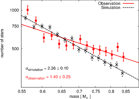
Figure 1: Global mass function in the mass range 0.55–0.85 M${\odot}$ for model ’M57R14.5’ without primordial mass segregation, which started with M=57000 M${\odot}$ and $R=$14.5 pc. The mass function at the start of the simulation was chosen to be a canonical Kroupa IMF, with $\alpha=2.3$ for the high-mass stars (see Sec. 4.1). The red solid line together with the red data points depicts the observed present-day mass function. The black, dotted line together with the black data points with a slope of $\alpha=2.36\pm 0.1$ shows the clusters mass function after an evolution of 11 Gyr. The error of the slope of mass function is derived from fitting. It is significantly steeper than the observed value. Hence, two-body relaxation is not able to deplete the mass function sufficiently to reproduce the observations, when starting from a non-segregated cluster on a circular orbit.

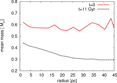
Figure 2: Mean stellar mass as a function of 3D radius for model ’M57R14.5’ without primordial mass segregation, which started with M=57000 M${\odot}$ and $R=$14.5 pc, in the mass range 0.55–0.85 M${\odot}$. Shown are the initial mean mass (red) and the final mean mass at $t=$11 Gyr (black) as function of projected radius. The decreasing mean mass with increasing distance from the cluster centre at $t=$11 Gyr indicates that dynamical mass segregation has happened in the cluster over time.

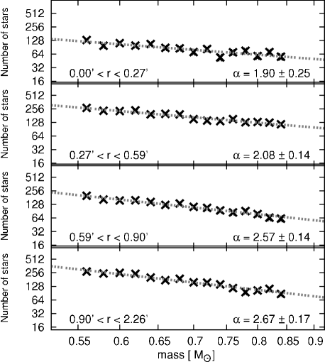
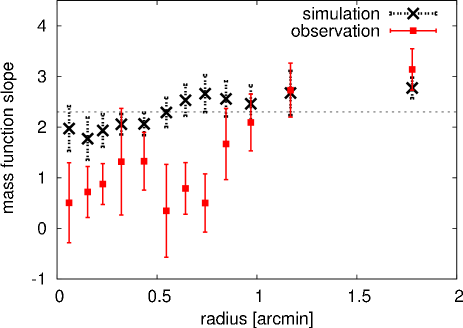
Figure 3: Top: the mass function in the mass range 0.55–0.85 M${\odot}$ for model ’M57R14.5’ without primordial mass segregation, which started with M=57000 M${\odot}$ and $R=$14.5 pc, after an evolution of 11 Gyr in various radial bins. From top to bottom, the panels represent the innermost to outermost regions shown in fig. 10 of Frank et al. (2012). The black dotted lines show power-law fits to the data. The radial ranges and best-fitting power-law slopes are indicated in each panel. The flattened slope within the inner parts with respect to the slope in the outer parts indicates that dynamical mass segregation has happened in the cluster. Bottom: the best-fitting mass function slopes, $\alpha$, derived in radial bins for the model mentioned above. The red squares are the observed values taken from Frank et al. (2012), and the black dots represent the result of the simulation after an evolution of 11 Gyr. The $\chi^{2}$ and $P$-value for this model are 36.24 and 0.001, respectively. This implies a probability of $10^{-3}$ that the data are represented by the model.

Table 1: Initial and final properties of all simulated star clusters starting with three different initial mass distributions. Column 1 gives the model name, in which the first two digit numbers after ‘M’ denote the initial mass in units of 1000 M${\odot}$ and the second two digit numbers denote the initial half-mass radius in parsec. For flattened models the first number in the model name is the adopted high-mass slope (see Section 4.3). Column 2 represents the adopted mass segregation parameter $S$. The mass segregation parameter changes in the range $S=0--0.95$. The following columns give the parameters of the simulated star clusters after 11 Gyr of evolution. The initial two-body relaxation time of models is presented in column 3. Column 4 gives the projected half-light radius $R_{hl}$. Column 5 gives the present-day total mass of the modelled cluster in the stellar mass range $0.55\leq m/\mbox{M}{\odot}\leq 0.85$. Column 6 is the present-day total mass of the cluster. The present-day slope of the mass function, $\alpha_{tot}$, for stars with masses between 0.55 and 0.85$\mbox{M}_{\odot}$ inside the projected radius $r=2.26$ arcmin, corresponding to $\approx 67$ pc, is presented in column 7. Columns 8 and 9 give the slope of the mass function inside and outside the half-light radius, respectively. The $\chi^{2}$ goodness-of-fit and corresponding $P$-values are presented in column 10 to compare the observed values of the slope of the mass function in different radial bins to those of the simulated models. The last column is the line-of-sight velocity dispersion of bright stars. Compared to the observational values given at the bottom, only the flattened models are an acceptable fit to Pal 4. Typical errors of the numerical values were obtained by repeating run M60R14 five times and are indicated in the header. The best-fitting models that agree within the uncertainties with all observational parameters are highlighted with boldface.

(1)	(2)	(3)	(4)	(5)	(6)	(7)	(8)	(9)	(10)	(11)
Model	$S$	$T_{rh}$	$R_{hl}$	$M_{measured}$	$M^{f}_{r<R_{t}}$	$\alpha_{tot}$	$\alpha_{in}$	$\alpha_{out}$	$\chi^{2}$($P$-value)	$\sigma_{los}$
		(Gyr)	(pc)	(M${\odot}$)	(M${\odot}$)					(kms-1)
			($\pm$2.1)	($\pm$105)	($\pm$1100)	($\pm$0.13)	($\pm$0.13)	($\pm$0.13)		($\pm$0.02)
Canonical-NS
M50R12	0	3.18	16.1	4894	26755	2.30	1.93	2.59	37.08 (0.001)	0.81
M55R12	0	3.28	16.1	5354	29372	2.28	2.11	2.62	36.84 (0.001)	0.84
M60R12	0	3.43	15.5	5920	32418	2.25	2.01	2.79	35.76 (0.001)	0.86
M50R14	0	4.01	16.6	4953	26762	2.25	1.87	2.58	32.52 (0.001)	0.76
M55R14	0	4.13	19.0	5236	28506	2.09	1.93	2.54	22.44 (0.021)	0.76
M60R14	0	4.32	16.8	5670	32320	2.31	2.17	2.68	32.28 (0.001)	0.84
M57R14.5	0	4.46	17.8	5550	30564	2.36	2.18	2.76	36.24 (0.001)	0.80
Canonical-S
M60R8	0.80	1.86	12.3	6449	32823	2.36	1.98	3.00	40.80 (0.001)	0.87
M60R8	0.95	1.86	15.8	6551	32683	2.17	1.68	2.91	25.80 (0.007)	0.79
M55R9	0.95	2.13	20.5	5565	27974	2.19	1.66	2.89	13.31 (0.273)	0.68
M60R10	0.50	2.60	14.0	6084	32203	2.21	1.94	2.71	35.50 (0.001)	0.87
M60R10	0.95	2.60	22.8	6278	31500	2.14	1.56	2.97	10.82 (0.460)	0.67
M57R10	0.95	2.55	22.1	5912	30025	2.25	1.86	2.97	18.96 (0.062)	0.67
Flattened
F0.5M57R14	0	4.23	20.5	5295	29435	1.26	1.12	1.81	16.87 (0.111)	0.79
F0.6M57R14	0	4.23	19.6	5870	30820	1.56	1.45	2.04	16.85 (0.112)	0.81
F0.7M57R14	0	4.23	18.6	6240	32292	1.76	1.60	2.27	20.76 (0.036)	0.84
F0.6M57R10	0.50	2.55	15.5	5888	30484	1.51	1.40	2.06	16.80 (0.114)	0.86
F0.6M55R10	0.70	2.49	16.8	5746	29418	1.54	1.23	2.22	8.88  (0.640)	0.80
F0.6M57R12	0.70	3.36	20.5	5875	30457	1.61	1.38	2.28	9.01  (0.620)	0.77
F0.6M57R10	0.90	2.55	20.3	5715	30231	1.41	0.79	2.35	13.80 (0.240)	0.76
Observations			18.4$\pm$1.1	5960$\pm$110	29800$\pm$800	1.4$\pm$0.25	0.89$\pm$0.39	1.87$\pm$0.24		0.87$\pm$0.18

All clusters in the first part of Table 1 start with a canonical Kroupa mass function but different initial half-mass radii and initial cluster masses.

As can be seen from the upper section of Table 1, the line-of-sight velocity dispersion in most of our computed models is about $0.8$ kms^-1, and therefore within the uncertainties of the observational value.

Furthermore, many models can reproduce Pal 14’s half-light radius (column 4) and its measured and total mass (column 5 and 6). We also calculate the global mass function slope for all models (column 7). Fig. 1 depicts the mass function of one example model after 11 Gyr of evolution and compares it with the observed data. Our simulations have typically $\alpha\simeq 2.2$ after 11 Gyr, which means only a mild decrease of the high-mass slope from the initial Kroupa value of $\alpha=2.3$. In contrast, the observed slope is $\alpha=1.4\pm 0.25$. Hence, the models starting with a canonical mass function are unable to reproduce the observed slope of the mass function of Pal 4 even when accounting for and statistical errors. This is a result of the long two-body relaxation time of the models and of the present-day cluster. This implies an evaporation time-scale which is significantly larger than the age of the cluster.

In Fig. 2, we plot the mean stellar mass, including the remnants, as a function of radius for the cluster M57R14.5, which is closest to Pal 4 among our non-segregated clusters. After 11 Gyr of evolution, the mean stellar mass decreases from $<$m$>\simeq 0.45M{\odot}$ at the centre of the cluster to $<$m$>\simeq 0.30M{\odot}$ at the half-mass radius. The decline of the mean mass with cluster radius shows the substantial degree of mass segregation that has been generated by dynamical evolution.

In order to test for mass segregation, we also measure the mass function as a function of radius of the modelled cluster. Fig. 3 shows the exponents of the best-fitting power laws fitted to the projected mass functions in four different radial bins. After 11 Gyr of evolution, the mass function steepens with increasing radius, from $\alpha\simeq 1.9\pm 0.25$ within a projected radius of $R=8.1$ pc to $\alpha\simeq 2.67\pm 0.17$ at the largest observed radius.

Fig. 3 shows that, while the mass function in the outer region of the non-segregated cluster is almost in agreement with the observations, this is not the case for the inner part of the cluster.

In order to measure the quality of the fit of the model to the observations, we employ the $\chi^{2}$ goodness-of-fit test defined as:

$$\chi^{2}=\sum_{i=1}^{N}\frac{(\alpha_{i,sim}-\alpha_{i,obs})^{2}}{\sigma_{i}^{2}},$$ (1)

where $\sigma_{i}^{2}=\sigma_{i,sim}^{2}+\sigma_{i,obs}^{2}$ is the uncertainty in the slope of the mass function including both observational as well as the simulated uncertainty. The sum runs over the $N=12$ radial bins. We obtain a value of $\chi^{2}=36.24$, which shows that, although the simulations show some degree of mass segregation, the primordially unsegregated clusters do not attain the observed degree of mass segregation and the discrepancy with the observations is extremely large. The corresponding $P$-value of 0.001 allows us to reject this model at the 99.9% confidence level. Similar results for the slope of the mass function are obtained for clusters with other initial radii and masses. These models do not undergo much mass loss due to being on circular orbits at a large Galactocentric radius, so their mass function can not fit after 11 Gyr of dynamical evolution. The main difference among these models lies in their final masses and radii. We therefore conclude that two-body relaxation alone cannot be responsible for the flattened mass function of Pal 4 and its segregated structure, if the post-gas expulsion re-virialized cluster had a canonical Kroupa IMF.

4.2 Canonical IMF with primordial mass segregation (canonical-S)

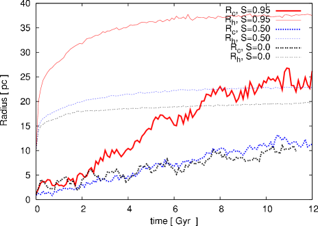
Figure 4: Evolution of the 3D half-mass radius (upper thick curves) and core radius (thin curves) for different degrees of primordial mass segregation with a canonical Kroupa IMF. The initial mass is 57000 M${\odot}$, and the initial half-mass radius is 10 pc for all models. Because of stellar evolution clusters experience a rapid expansion such that clusters with higher degrees of primordial mass segregation experience a larger jump in the half-mass radius within the first 100 Myr of evolution. The rising core radius shows that the cluster is still in the pre-core-collapse phase.

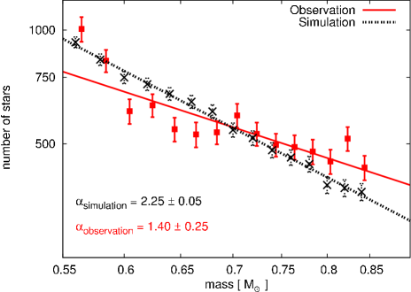
Figure 5: The same as Fig. 1, but for a primordially mass-segregated cluster with a canonical Kroupa IMF. The initial mass of this particular model (M57R10) is 57000 M${\odot}$, the initial half-light radius is 10 pc, and the mass segregation parameter is set to $S=0.95$. Clusters with such a strong degree of primordial mass segregation are still not able to reproduce the observed flat mass function (see the text for more explanation).

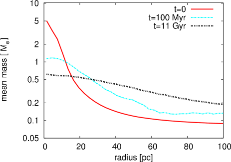
Figure 6: The same as Fig. 2, but here we started with a primordially mass-segregated cluster with a canonical Kroupa IMF. The initial mass of this particular model (M57R10) is 57000 M${\odot}$, the initial half-light radius is 10 pc and the mass segregation parameter is set to $S=0.95$. The mean mass profile at $t=100$ Myr after the early stellar evolution of massive stars is also plotted.

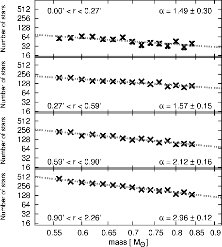
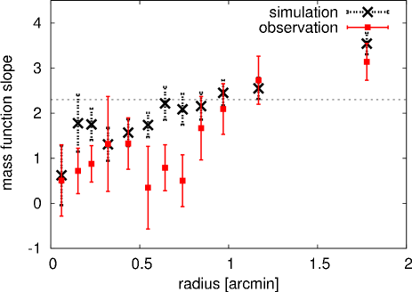
Figure 7: The same as Fig. 3, but for a primordially mass-segregated cluster with a canonical Kroupa IMF. The initial mass of this particular model (M57R10) is 57000 M${\odot}$, the initial half-light radius is 10 pc and the mass segregation parameter is set to $S=0.95$. As can be seen, the mass function steepens with increasing radius, and the mass function slopes in each bin are marginally compatible with the observed values. The $\chi^{2}$ value for this model is 18.96 corresponding to a probability of 6.2% that the data can be represented by the model.

In order to understand whether primordial mass segregation helps to reconcile the inconsistency between observations and simulations, we calculated a number of models starting with primordial mass segregation. That is, the post-gas expulsion re-virialaized cluster is assumed to be mass segregated with an overall canonical IMF.

The code McLuster allows to initialize any degree of primordial mass segregation (hereafter, $S$) to all available density profiles. $S=0$ means no segregation (’NS’ in Table 1) and $S=1$ refers to full segregation. McLuster uses the routine described in Baumgardt, De Marchi, & Kroupa (2008) to segregate the clusters. This routine allows to maintain the desired density profile when increasing the degree of mass segregation while also making sure that the cluster is in virial equilibrium. For a fully segregated cluster, the highest mass star occupies the orbit with the lowest energy.

To allow for a better comparison with the models from Sec. 4.1, we set up clusters with various degrees of mass segregation in the range $S=0.5-0.95$, the same range of initial cluster masses, but with smaller initial half-mass radii. The reason that we chose a smaller initial radius is the expansion due to both dynamical and stellar evolution. In the first few Myr of a cluster’s life, the mass loss is dominated by stellar evolution of massive stars in the core and leads to a rapid expansion in the size of the cluster. Fig. 4 shows the evolution of the 3D half-mass radius and the core radius for different values of the mass segregation parameter over the entire evolution of the cluster. The growing core radius shows that the cluster is far from the core collapse.

The results of the simulated models with primordial mass segregation are shown in Table 1 and Figs. 5–7. Even by selecting very high values of primordial segregation, the present-day global mass function of Pal 4 cannot be reproduced. Since the whole cluster is included within 2.26 arcmin in the calculation of the global mass function, and since the overall mass function did not change for the segregated clusters (because we just distributed the stars differently according to their mass), one should expect to end with the same global (i.e. within $R=2.26$ arcmin) mass function as in the unsegregated case. Also, distant globular clusters undergo very little mass loss due to tidal interaction. Almost 45% of the initial mass is lost owing to early stellar evolution. From Table 1 it can then be estimated that dynamical interactions lead to about 15% additional mass loss after 11 Gyr evolution.

Fig. 6 shows the mean stellar mass, including the remnants, as a function of 3D radius for the modelled cluster ’M57R10’ with $S=0.95$. The rapid fall in mean mass during the first 100 Myr is due to stellar evolution of massive stars, which is the dominant process in the early evolution of the clusters. Thereafter, the change in mean mass continues more slowly. The final mean mass profile at 11 Gyr shows that the mean stellar mass decreases from $<$m$>\simeq 0.62M{\odot}$ at the centre of the cluster to $<$m$>\simeq 0.43M{\odot}$ at the 3D half-mass radius of 37 pc.

By comparing Figs  3 and 7, it can be seen that the mass function slopes in different radial bins are closer to the observed values for the initially segregated models than the unsegregated ones. This is confirmed by the lower $\chi^{2}$ value of 18.96 for this model. The corresponding $P$-value of 0.062 allows us to reject this model at the 93% confidence. Moreover, in the segregated models, the amount of mass function flattening does not depend on the amount of mass segregation.

According to Table 1, some of the mass segregated models such as ’M55R9’, ’M60R10’, and ’M57R10’ have $P$-values of 0.273, 0.460 and 0.062, respectively, so these models cannot be excluded given the data of radial structure of the slope of the mass function, but the difference between the observed and calculated values of $\alpha_{tot}$ are significant for both inside and outside the half-light radius. The slope of the mass function in all models is far from the observed value of Pal 4, though, even when accounting for observational and statistical errors. Moreover, we find that the values for the present-day total mass of the modelled clusters M55R9’ and ’M60R10’ in the stellar mass range $0.55\leq m/\mbox{M}{\odot}\leq 0.85$ (column 5 of Table 1) are not compatible with the observed values. A glimpse on the last column of Table 1 shows that if we account for the statistical and observational errors, the line-of-sight velocity dispersion for these models is marginally compatible with the observed value. Therefore it is clear that we will not be able to fit the observations if we start with a Kroupa/Salpeter mass function.

4.3 Flattened IMF

Figure 8: The same as Fig. 1, but here we started with a flattened mass function with a slope of $\alpha=1.6$ above 0.5 M${\odot}$ and $\alpha=0.6$ below 0.5 M${\odot}$. The initial mass of this particular model (F0.6M57R14) is 57000 M${\odot}$, the initial half-light radius is 14 pc. Further properties of the cluster after 11 Gyr of evolution are given in Table 1.

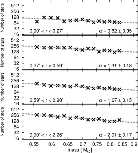
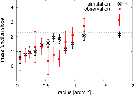
Figure 9: The same as Figure 3, but here we started with a flattened mass function with a slope of $\alpha=1.6$ above 0.5 M${\odot}$ and $\alpha=0.6$ below 0.5 M${\odot}$. The initial mass of this particular model (F0.6M57R14) is 57000 M${\odot}$, the initial half-light radius is 14 pc. Further properties of the cluster after 11 Gyr of evolution are given in Table 1. The $\chi^{2}$ value for this model is 16.80, corresponding to a probability of 88.6% for rejecting the model.

So far, we have shown that clusters starting with a Kroupa/Salpeter slope of $\alpha=2.3$ at the high-mass end cannot reproduce the observed slope of the mass function well. The smallest slope that can be achieved from these models is about 2.0, while the observed slope is $\alpha=1.40\pm 0.25$. In this section we present a number of models starting with a flatter IMF to see whether it is possible to make up for the discrepancy in $\alpha$.

One way to achieve such a flat mass function is if the cluster was born mass segregated and embedded in a primordial gas cloud. In such a case, the early phase of gas expulsion can be very violent, depending on the exact initial conditions of its parent gas cloud (Baumgardt & Kroupa, 2007; Baumgardt, Kroupa, & Parmentier, 2008; Parmentier et al., 2008; Marks, Kroupa, & Baumgardt, 2008; Dabringhausen, Fellhauer, & Kroupa, 2010; Banerjee & Kroupa, 2013). The ejection and distribution of the remaining cloud gas is the natural outcome of the stellar winds of massive stars, and of supernovae explosions. This early rapid mass loss changes the gravitational potential, and consequently causes a cluster to expand. Such expansion leads to the rapid dissolution of low-concentration clusters. For initially mass-segregated clusters, the mass lost due to the evolution of massive stars is removed preferentially from the cluster’s inner regions, and the early expansion of the cluster is stronger and potentially more destructive than when the same amount of mass is lost in a non-segregated cluster.

Marks, Kroupa, & Baumgardt (2008) suggested that an initially mass-segregated cluster loses preferentially low-mass stars during the gas-expulsion phase, which would leave the cluster with a flattened mass function. Therefore, a globular cluster’s evolution over a Hubble time can be strongly affected by this early evolutionary processes (Marks & Kroupa, 2010).

Assuming that a certain flattening of the mass function slope has happened within the first 100 Myr of the cluster’s evolution, we have performed a series of $N$-body simulations for models with various flattened initial slopes of the mass function instead of the canonical IMF (Table 1). The effect of early evolutionary processes on the long-term evolution of clusters cannot be easily computed in a direct way for a globular cluster of the pre-gas expulsive mass of Pal 4, because clusters can lose a large fraction of their birth stellar population as a result of gas expulsion. The initial state of our models therefore ought to be understood as being the re-virialized state of a post-gas expulsion cluster (Banerjee & Kroupa, 2013).

Since stars with masses larger than 5 M${\odot}$ will have died or turned into compact remnants within the first 100 Myr, the maximum mass in the mass spectrum was set to 5 M${\odot}$, instead of 100 M${\odot}$. Because of the low escape velocity from Pal 4, it is reasonable to assume a 0 per cent retention fraction for neutron stars and black holes that form during the simulation.

We have chosen three sets of slopes for the mass function: $\alpha_{a}=\{1.7,0.7\}$, $\alpha_{b}=\{1.6,0.6\}$ and $\alpha_{c}=\{1.5,0.5\}$, where the first number in each set is the slope of the mass function for stars more massive than 0.5 M${\odot}$ and the second one is for low-mass stars (for comparison, the Kroupa IMF is $\alpha=\{2.3,1.3\}$). The first column in Table 1 shows the name of the simulated models. For example, F0.6M57R14 represents a flattened model with a slope of $\alpha_{b}=\{1.6,0.6\}$, an initial mass of 57000 M${\odot}$, and an initial (i.e. post-gas expulsion re-virialized) half-mass radius of 14 pc.

The results are summarized in the lower section of Table 1. We find that a particular model (F0.6M57R14) without primordial segregation ($S=0$) can reproduce the present day total mass and half-light radius of Pal 4 better than the scenarios mentioned above. The global mass function slope of this model after 11 Gyr of evolution is $\alpha=1.56\pm 0.07$, which is compatible with the observed value within the uncertainty (see also Fig. 8). Moreover, according to Table 1, all other present day properties of this model are in good agreement with the observed values.

In Fig. 9 we plot the mass function slope as a function of radius for the best-fitting model, F0.6M57R14. We see that mass segregation has taken place, in addition to our artificial flattening of the mass function, by about the same amount as in the non-flattened case (Fig. 3).

Fig. 9 shows the mass function and power-law fits to the mass distributions for different radii. As can be seen, the slope of the inner part is compatible with the observed value. The average values of the mass function slopes in the outer regions are compatible with the observed values within the uncertainties, since we obtain $\chi^{2}=16.8$, which corresponds to a $P$-value of 0.114. This means that the model can be just rejected with 88.6 per cent confidence. That is not very strong and this model can be acceptable.

This agreement can be increased by adding mass segregation to the initial configuration. Such a cluster with a flattened mass function and some left-over mass segregation ($S\geq 0.7$) would be the natural outcome of a primordially strongly mass-segregated cluster which expelled its gas and preferentially lost its low-mass stars. As shown in Figs 10 and 11, the agreement can be made almost perfect, since we obtain $\chi^{2}=8.9$, which corresponds to a $P$-values of 0.640.

In fact, in models with flattened mass function, the slope of the stellar mass function in the mass range $0.55\leq m/\mbox{M}{\odot}\leq 0.85$ is lowered across the cluster in all radial bins. Because of the addition of mass segregation, the slope of the mass function in the outer radial bins ($r>0.7$ arcmin) increases, while in the inner bins ($0.7>r>0.3$ arcmin) it decreases. This leads to a better agreement with the observations.

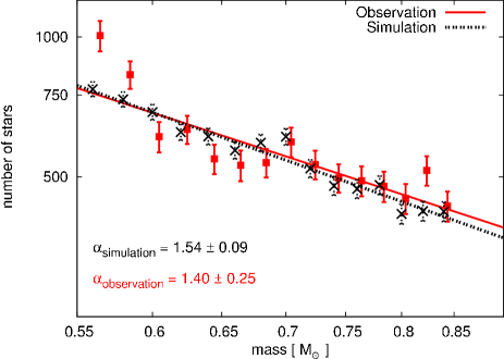
Figure 10: The same as Fig. 1, but here we started with a primordially segregated cluster with a flattened mass function with a slope of $\alpha=1.6$ above 0.5 M${\odot}$ and $\alpha=0.6$ below 0.5 M${\odot}$ . The initial mass of this particular model (F0.6M55R10) is 55000 M${\odot}$, the initial half-light radius is 10 pc, and the mass segregation parameter is set to $S=0.70$. Further properties of the cluster after 11 Gyr of evolution are given in Table 1.

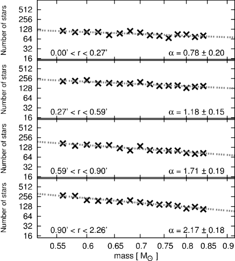
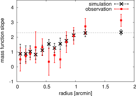
Figure 11: The same as Fig. 3, but here we started with a flattened mass function with a slope of $\alpha=1.6$ above 0.5 M${\odot}$ and $\alpha=0.6$ below 0.5 M${\odot}$. The initial mass of this particular model (F0.6M55R10) is 55000 M${\odot}$, the initial half-light radius is 10 pc and the mass segregation parameter is set to $S=0.70$. Further properties of the cluster after 11 Gyr of evolution are given in Table 1. The $\chi^{2}$ value for this model is 8.9, corresponding to a $P$-value of 0.64.

4.4 The effect of unresolved binaries

Binary stars, either primordial or dynamically formed during close encounters between single stars, can affect the observational parameters of a star cluster, such as the velocity dispersion and the mass function. Unfortunately, binaries slow down direct $N$-body computations enormously because timesteps have to be very small for their integration, such that most numerical investigations neglect binaries completely. Star cluster models with a 100% primordial binary fraction and full realistic binary star distribution function have been presented by Kroupa (1995a, b, c) and Kroupa, Aarseth, & Hurley (2001). The binaries could also have an impact on the dynamical evolution of the cluster, and might therefore allow the initial conditions to be more compact (allowing rapid mass segregation) followed by a period of binary-driven expansion (Wilkinson et al., 2003).

In our analysis we did not take into account the effects of unresolved binaries on the determination of the mass function so far. An unresolved binary consisting of two main-sequence stars will have a combined colour somewhere in between the colours of the two components, and a magnitude brighter than that of a single-star main sequence at this combined colour (Kroupa & Tout, 1992). If the binarity is not taken into account in the determination of stellar masses, the combined system will be assigned a mass that is larger than the mass of the two single stars. This causes an unrealistic flattening in the mass function slope (Kroupa, Gilmore, & Tout, 1991; Kroupa, Tout, & Gilmore, 1993).

The magnitude of this effect depends on the fraction of unresolved binaries and the mass distribution of the binary components. Here, we investigate the effect of binaries on measured mass function slopes by populating evolved McLuster models of Pal 4 with a varying fraction of binaries,

$$f_{bin}=\frac{N_{bin}}{(N_{bin}+N_{single})},$$ (2)

following the method outlined in Frank et al. (2012). $N_{bin}$ is the number of binary systems in the cluster and $N_{single}$ is the number of single stars. We add binaries following a Kroupa period distribution and a thermal eccentricity distribution (Kroupa 1995b), and the binary components with different masses were paired randomly for stars with $m\leq 5M{\odot}$ after choosing both companion masses independently and randomly from the IMF. For massive stars with $m\geq 5M{\odot}$ the pairing rules change and they tend to prefer more similar-mass companions (Sana & Evans, 2011).

We assume different values for the binary fraction ranging from 10 to 90 per cent, to evaluate the effect of a population of unresolved binaries on the slope of the mass function. To obtain the mass function of the cluster members, we do the following procedure.

(i) We derive the luminosity of each star in the modelled cluster and add up the luminosities of the two components for each binary system.

(ii) In order to turn the combined luminosity back into a mass, we generate a large cluster model, astrophysically evolve it to an age of 11 Gyr and derive a relation between luminosity and mass from all single stars in the cluster. Using this relation, we then convert the luminosity of each binary back into a mass estimate.

It should be noted that, in order to be compatible with the observations for Pal 4 by Frank et al. (2012), we restrict the sample from which we derive the transformation to systems for which at least one component is a main-sequence, sub-giant branch, or red giant branch star.

We first derive the system mass function that is the mass function for binaries and single stars. It is shown in Fig. 12 as $\alpha_{SYS}$. Then, in order to compare we calculate the mass function for the single stars and the components of the binaries ($\alpha_{S}$).

As can be seen in Fig. 12, the slope of the mass function in the low-mass range decreases as the binary fraction increases, while there is no significant change in the high-mass end which is the observed range in this paper. A high binary fraction, say 90%, which is most probably not realistic for an evolved cluster like Pal 4, can make the mass function extremely flattened (i.e. $\alpha_{1SYS}\simeq 0.24$) in the low-mass range $m/M{\odot}\leq 0.5$. This confirms the results of Kroupa, Gilmore, & Tout (1992), Kroupa, Tout, & Gilmore (1993), Weidner, Kroupa, & Maschberger (2009) and Khalaj & Baumgardt (2013) that even under extreme circumstances (100% binaries or higher order multiples), the effect of unresolved multiple systems on the power-law index of the mass function slope is small ($\leq 0.1$) at the high-mass end.

A decrease of $\alpha$ at the low-mass end can be expected since many low-mass stars will be hidden in binaries with more massive companions. However, the effect at the high-mass end is small, even for a binary fraction of 90%. With a flattening of $\approx 0.2$ it is of the order of the uncertainties in the observations. We therefore conclude that unresolved binaries cannot be responsible for the flattening of the mass function in the observed mass range in Pal 4.

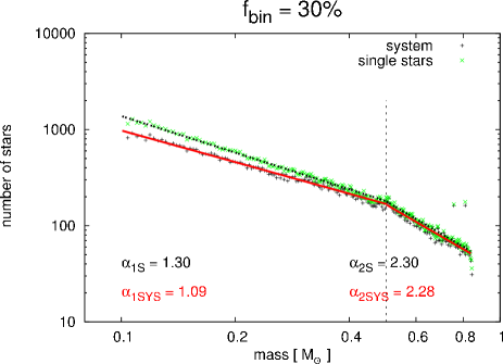
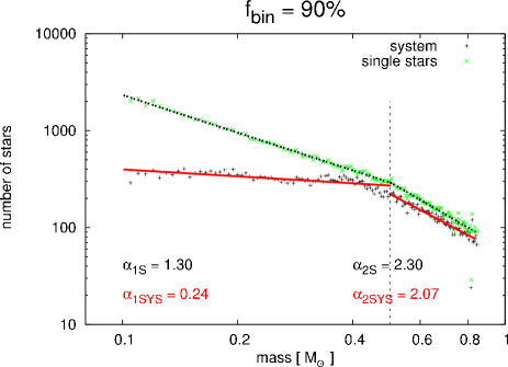
Figure 12: The effect of increasing the binarity on the measured mass function. In the top panel, the binary fraction is $f_{bin}=30\%$ and in the bottom panel it is $f_{bin}=90\%$. The vertical dashed line which corresponds to $m_{break}=0.5M{\odot}$ shows the point at which the Kroupa canonical IMF has a break. The black, dotted lines show the best fit to the mass function of low- and high-mass stars assuming all binaries to be resolved into their components. The corresponding values for the slopes ($\alpha_{1S}$ and $\alpha_{2S}$) in both low- and high-mass ranges are compatible with a Kroupa IMF. The solid red lines show the best fit to the mass function considering the effect of unresolved binaries. According to the calculated values for the slopes ($\alpha_{1SYS}$ and $\alpha_{2SYS}$), a high binary fraction can severely affect the measured mass function slope in the low-mass range, below $m=0.5M{\odot}$, but it has little effect above this value .

5 Conclusions

This paper is the second study in which we model the dynamical evolution of a Galactic globular cluster over its entire lifetime by direct $N$-body simulations on a star-by star basis. While we focused on Pal 14 in Paper I (Zonoozi et al., 2011), we here investigate the diffuse outer halo globular cluster Pal 4 using the $N$-body code nbody6 (Aarseth, 2003).

Recent observational work on Pal 4 (Frank et al., 2012) has shown that the global mass function slope in the mass range 0.55-0.85 M${\odot}$ is $\alpha=1.4\pm 0.25$, i.e. significantly shallower than a canonical mass function slope of about 2.3 (Kroupa, 2001). Similar results have been found for a number of Milky Way globular clusters (see, e.g., De Marchi et al. 2007; Jordi et al. 2009; Paust et al. 2010; Frank et al. 2012; Hamren et al. 2013). Interestingly, Frank et al. (2012) also found that the slope of the mass function steepens with radius from a slope of $\alpha\leq 1$ inside about $1.3r_{h}$ to $\alpha\geq 2.3$ at the largest observed radii, indicating the presence of mass segregation in Pal 4 and therefore constraining numerical models much more than our previous target Pal 14 could do.

A preferential loss of low-mass stars due to two-body relaxation would be a natural explanation for the observed mass function depletion (Baumgardt & Makino, 2003). However, for diffuse outer halo clusters such as Pal 4 and Pal 14 (i.e., a low mass together with a large half-mass radius), the present-day two-body relaxation time is of the order of a Hubble time. Therefore, relaxation should be inefficient in these clusters and the observations should be an indication for primordial mass segregation. Alternatively the cluster could have been more compact in the past such that relaxation was more important at that time. To test these scenarios, we have tried to find the best possible evolutionary model for Pal 4 by running a set of models with varying initial half-mass radii and total masses, until we got an adequate fit to the observed structural parameters.

While it is relatively straightforward to find initial models which reproduce the observed structural parameters of Pal 4, i.e. half-light radius, total mass and velocity dispersion, it is very difficult if not impossible to reproduce its global mass function and degree of mass segregation. Because the models have to start with a comparatively low mass and large half-mass radius of about 55000 M${\odot}$ and 10 pc, low-mass star depletion and mass segregation are very ineffective in these clusters. We showed that models evolving on circular orbits, starting with a Kroupa IMF, and without primordial mass segregation do not produce enough depletion in the slope of the mass function. In addition, these models do not develop enough mass segregation within the cluster lifetime to match the observations. It should be noted that the current conclusions are based on the assumption of a circular orbit for Pal 4. The orbit of Pal 4 is unknown however. In the case of an eccentric orbit the Galactic field changes with time, which could significantly affect the dynamical evolution of Pal 4.

We also find that the present-day global mass function slope of Pal 4 cannot be reproduced in models starting with a canonical but primordially segregated IMF, not even by using very high degrees of primordial segregation. Models starting with a flattened IMF reach enough depletion in the global mass function to be compatible with the observations. However, the radial variation of the mass function slope is significantly better reproduced when we include both a flattened IMF and primordial mass segregation.

This is similar to our findings from Paper I (Zonoozi et al., 2011), where we concluded that Pal 14 must have undergone one of two scenarios:

1. the observed mass function may be a result of dynamical evolution starting from a canonical Kroupa IMF with a high degree of primordial mass segregation;
   

2. the observed mass function may be the result of an already established non-canonical IMF depleted in low-mass stars, which might have been obtained during a violent early phase of gas-expulsion of an embedded cluster with primordial mass segregation (Marks & Kroupa, 2010).

Now, for Pal 4 we can exclude the first scenario as we have observations covering larger parts of the cluster and hence have more precise knowledge of the present-day global mass function and the degree of mass segregation.

This leaves us with the assumption that the peculiar mass function and the cluster’s unusual extent have been imprinted on Pal 4 during its very early lifetime. The inferred initial half-light radius of about 10 pc is significantly larger than the present-day half-light radii of most globular clusters, which are narrowly distributed around 3 pc (Jordán et al., 2005). This could be a footprint of the weaker external tidal force of Pal 4’s host galaxy during its formation. The Galactic tidal field, which we here model as being static, has evolved significantly since Pal 4’s birth and might have been much weaker 11 Gyr ago. The cluster might have also been born in a now detached/disrupted dwarf galaxy.

Alternatively, since star clusters lose more mass during pericentric passages on eccentric orbits, and undergo stronger expansion due to the weaker tidal fields at larger Galactic radii (Madrid, Hurley, & Sippel, 2012), an eccentric cluster orbit might have had an important influence on Pal 4’s evolution, as it could have had a much smaller initial size and significantly higher mass. We leave this scenario for an upcoming paper to be investigated in detail (Küpper et al., in preparation).

References

- Aarseth (2003) Aarseth S. J., 2003, Gravitational N-Body Simulations, Cambridge University Press, Cambridge
- Allen & Santillan (1991) Allen C., Santillan A., 1991, Rev. Mex. Astron. Astrofis, 22, 255
- Allison et al. (2009) Allison R. J., Goodwin S. P., Parker R. J., de Grijs R., Portegies Zwart S. F., Kouwenhoven M. B. N., 2009, ApJ, 700, L99
- Banerjee & Kroupa (2013) Banerjee S., Kroupa P., 2013, ApJ, 764, 29
- Bastian et al. (2008) Bastian N., Gieles M., Goodwin S. P., Trancho G., Smith L. J., Konstantopoulos I., Efremov Y., 2008, MNRAS, 389, 223
- Baumgardt & Makino (2003) Baumgardt H., Makino J., 2003, MNRAS, 340, 227.
- Baumgardt & Kroupa (2007) Baumgardt H., Kroupa P., 2007, MNRAS, 380, 1589
- Baumgardt, De Marchi, & Kroupa (2008) Baumgardt H., De Marchi G., Kroupa P., 2008, ApJ, 685, 247
- Baumgardt, Kroupa, & Parmentier (2008) Baumgardt H., Kroupa P., Parmentier G., 2008, MNRAS, 384, 1231
- Bonnell et al. (1997) Bonnell I. A., Bate M. R., Clarke C. J., Pringle J. E., 1997, MNRAS, 285, 201
- Bonnell et al. (2001) Bonnell I. A., Clarke C. J., Bate M. R., Pringle J. E., 2001, MNRAS, 324, 573
- Bonnell & Davies (1998) Bonnell I. A. & Davies M. B., 1998, MNRAS, 295, 691
- Bonnell & Bate (2006) Bonnell I. A., Bate M. R., 2006, MNRAS, 370, 488
- Burbidge & Sandage (1958) Burbidge E. M., Sandage A., 1958, ApJ, 127, 527
- Christian & Heasley (1986) Christian C. A., Heasley J. N., 1986, ApJ, 303, 216
- de Grijs et al. (2002) de Grijs R., Gilmore G. F., Johnson R. A., Mackey A. D., 2002, MNRAS, 331, 245
- de Grijs (2010) de Grijs R., 2010, Philos. Trans. R. Soc. A: Math. Phys. Eng. Sci., 368, 693
- Dabringhausen, Fellhauer, & Kroupa (2010) Dabringhausen, J., Fellhauer, M., & Kroupa, P. 2010, MNRAS, 403, 1054
- De Marchi et al. (2007) De Marchi G., Paresce F., Pulone L., 2007, ApJ, 656, L65
- Dotter et al. (2008) Dotter A., Chaboyer B., Jevremović D., Kostov V., Baron E., Ferguson J. W., 2008, ApJS, 178, 89
- Fellhauer, Wilkinson, & Kroupa (2009) Fellhauer M., Wilkinson M. I., Kroupa P., 2009, MNRAS, 397, 954
- Fischer et al. (1998) Fischer P., Pryor C., Murray S., Mateo M., Richtler T., 1998, AJ, 115, 592
- Frank et al. (2012) Frank M. J., Hilker M., Baumgardt H., Côté P., Grebel E. K., Haghi H., Küpper A. H. W., Djorgovski S. G., 2012, MNRAS, 423, 2917
- Giersz & Heggie (2011) Giersz M., Heggie D. C., 2011, MNRAS, 410, 2698
- Gouliermis et al. (2004) Gouliermis D., Keller S. C., Kontizas M., Kontizas E., Bellas-Velidis I., 2004, A&A, 416, 137
- Gouliermis, de Grijs, & Xin (2009) Gouliermis D. A., de Grijs R., Xin Y., 2009, ApJ, 692, 1678
- Gürkan, Freitag, & Rasio (2004) Gürkan M. A., Freitag M., Rasio F. A., 2004, ApJ, 604, 632
- Hamren et al. (2013) Hamren K. M., Smith G. H., Guhathakurta P., Dolphin A. E., Weisz D. R., Rajan A., Grillmair C. J., 2013, AJ, 146, 116
- Harris (1996) Harris W. E., 1996, AJ, 112, 1487 (arXiv:1012.3224)
- Heggie & Hut (2003) Heggie D., Hut P., 2003, The Gravitational Million Body Problem. Cambridge University Press, Cambridge
- Hillenbrand (1997) Hillenbrand L. A., 1997, AJ, 113, 1733
- Hillenbrand & Hartmann (1998) Hillenbrand L. A., Hartmann L. W., 1998, ApJ, 492, 540
- Hurley, Pols & Tout (2000) Hurley J. R., Pols O. R., Tout C. A., 2000, MNRAS, 315, 543
- Hurley, Tout & Pols (2002) Hurley J. R., Tout C. A., Pols O. R., 2002, MNRAS, 329, 897
- Irrgang et al. (2013) Irrgang A., Wilcox B., Tucker E., Schiefelbein L., 2013, A&A, 549, A137
- Jordán et al. (2005) Jordán A., et al., 2005, ApJ, 634, 1002
- Jordi et al. (2009) Jordi K. et al., 2009, AJ, 137, 4586
- Khalaj & Baumgardt (2013) Khalaj P., Baumgardt B., 2013, MNRAS, 434, 3236
- King (1966) King I. R., 1966, AJ, 71, 276
- Klessen (2001) Klessen R. S., 2001, ApJ, 556, 837
- Kroupa, Gilmore, & Tout (1991) Kroupa P., Gilmore G., Tout C. A., 1991, MNRAS, 251, 293
- Kroupa & Tout (1992) Kroupa P., & Tout C. A., 1992, MNRAS, 259, 223
- Kroupa, Gilmore, & Tout (1992) Kroupa P., Gilmore G., Tout C. A., 1992, AJ, 103, 1602
- Kroupa, Tout, & Gilmore (1993) Kroupa P., Tout C. A., Gilmore G., 1993, MNRAS, 262, 545
- Kroupa (1995a) Kroupa P., 1995a, MNRAS, 277, 1491
- Kroupa (1995b) Kroupa P., 1995b, MNRAS, 277, 1507
- Kroupa (1995c) Kroupa P., 1995c, MNRAS, 277, 1522
- Kroupa (2001) Kroupa P., 2001, MNRAS, 322, 231
- Kroupa, Aarseth, & Hurley (2001) Kroupa P., Aarseth S., Hurley J., 2001, MNRAS, 321, 699
- Kroupa (2002) Kroupa P., 2002, Science, 295, 82
- Kroupa (2008) Kroupa, P. 2008, in Aarseth S. J., Tout C. A., Mardlingin R. A., eds, Lecture Notes in Physics, Vol. 760, The Cambridge N-Body Lectures. Springer-Verlag, Berlin, p. 181
- Kroupa et al. (2013) Kroupa P., Weidner ., Pflamm-Altenburg J., Thies I., Dabringhausen J., Marks M., Maschberger T., 2013, Stellar Systems and Galactic Structure, Vol. 5. Springer-Verlag, Berlin
- Küpper et al. (2011) Küpper A. H. W., Maschberger T., Kroupa P., Baumgardt H., 2011, MNRAS, 417, 2300
- McMillan, Vesperini, & Portegies Zwart (2007) McMillan S. L. W., Vesperini E., Portegies Zwart S. F., 2007, ApJ, 655, L45
- Madrid, Hurley, & Sippel (2012) Madrid J. P., Hurley J. R., Sippel A. C., 2012, ApJ, 756, 167