Monte Carlo Null Models for Genomic Data

Abstract

As increasingly complex hypothesis-testing scenarios are considered in many scientific fields, analytic derivation of null distributions is often out of reach. To the rescue comes Monte Carlo testing, which may appear deceptively simple: as long as you can sample test statistics under the null hypothesis, the $p$-value is just the proportion of sampled test statistics that exceed the observed test statistic. Sampling test statistics is often simple once you have a Monte Carlo null model for your data, and defining some form of randomization procedure is also, in many cases, relatively straightforward. However, there may be several possible choices of a randomization null model for the data and no clear-cut criteria for choosing among them. Obviously, different null models may lead to very different $p$-values, and a very low $p$-value may thus occur due to the inadequacy of the chosen null model. It is preferable to use assumptions about the underlying random data generation process to guide selection of a null model. In many cases, we may order the null models by increasing preservation of the data characteristics, and we argue in this paper that this ordering in most cases gives increasing $p$-values, that is, lower significance. We denote this as the null complexity principle. The principle gives a better understanding of the different null models and may guide in the choice between the different models.

, and

1 Introduction

Increasingly, Monte Carlo methods are needed to provide answers to important scientific questions, particularly in the rapidly advancing field of genomics. For better or worse, these questions are often framed within the formalism of statistical hypothesis testing. In many cases, Monte Carlo hypothesis testing techniques such as permutation testing are the only options.

Conceptually, these methods share an appealing clarity: As long as you can sample test statistics under the null hypothesis, the $p$-value is just the proportion of sampled test statistics that exceed the observed test statistic. One of our main aims is to show that the apparent simplicity of randomization hypothesis testing can be very deceptive. In the following, we use null model as a general term for the distribution of the resampled data (e.g., using random permutations), and we use null distribution to denote the distribution of the test statistic under the null model. Even though there is a highly developed theory of classical hypothesis testing (e.g., Lehmann and Romano (2005)), new practical and methodological problems appear when we need to resort to Monte Carlo testing:

• The question of interest may be unavoidably vague, so that it is not obvious how to translate it into a precise mathematical formulation.

• There may be several possible choices of a randomization null model and no clear-cut criteria for choosing among them (except possibly conservativeness arguments for choosing the null model giving the largest $p$-values).

• A full specification of the null hypothesis consists of both the null model and the question of interest. This complicates the interpretation of a rejection of the null hypothesis—the question of interest may not really have been answered if the null model is inadequate.

• There may be several possible choices of test statistic and no clear-cut criteria for choosing one (except possibly power considerations).

If unresolved, these problems may degrade the reproducibility and transparency of investigations, as well as lead to false research findings. There has lately been an increasing focus on how to make science more reproducible, especially in the field of computational biology (Ioannidis et al. (2008); Noseda and McLean (2008); Mesirov (2010); Sandve et al. (2013b)). Also, due to the increased prevalence of data-driven science (Kell and Oliver, 2004) through increased availability of public data and more accessible and efficient analytical tools, there has also been a heated discussion on whether a large proportion of published research findings are false (Ioannidis (2005); Goodman and Greenland (2007)). We discuss this topic further in the remainder of this paper. Our main application of interest is genomics and the Genomic HyperBrowser (Sandve et al., 2010, 2013a) where choosing the correct null model is a major issue. We have discussed null models in ecology in a companion report, Ferkingstad, Holden and Sandve (2013). Several examples show that the choice of a null model can strongly affect the resulting $p$-values. We state that ordering the null models according to increasing preservation may imply an ordering of the statistical significance. Further, if the null models are not able to capture the essential structural properties of data, this may lead to false findings.

We proceed as follows: Section 2 discusses general problems of randomization null models. Section 3 presents null model preservation hierarchies and significance orderings. Sections 4–6 illustrate several different null models within genomics: Section 4 considers null models for the location of transcription factor binding sites, Section 5 shows that genetic properties have a tendency to cluster along the genome, while Section 6 illustrates that we may get false rejections with too simple null models using simulated data of points and segments in genomic tracks. Finally, Section 7 provides a general discussion and some concluding remarks and recommendations.

For the genomics case studies described in Sections 4–6 we have used $q$-values (Storey, 2002) to correct for multiple testing. Assume that we test $m$ hypotheses where $p_{(1)}\leq p_{(2)}\leq\cdots\leq p_{(m)}$ are the ordered, observed $p$-values, $R$ is the number of rejected null hypotheses, and $V$ is the (unknown) number of falsely rejected null hypotheses. The false discovery rate (FDR) (Benjamini and Hochberg, 1995) is then defined as FDR $=\mathrm{E}(V/R)$. For each test, the corresponding $q$-value is defined as the minimum FDR at which the test is called significant. Let $\pi_{0}$ be the proportion of tests that are truly null (Langaas, Lindqvist and Ferkingstad, 2005) and $q_{(i)}$ the $q$-value for the test with $p$-value $p_{i}$. Then, we may estimate $q_{(i)}$ by

$$\hat{q}_{(i)}=\min_{i\leq j\leq m}m*\hat{\pi}_{0}*p_{(j)}/j,$$

where $\hat{\pi}_{0}$ is an estimate of $\pi_{0}$. Thus, the main inputs to this multiple testing method are the observed $p$-values together with an estimate of $\pi_{0}$. To estimate $\pi_{0}$, we have used the robust estimator of Pounds and Cheng (2006), since this is very computationally efficient and can be shown to be conservative in many realistic settings. For a general discussion of multiple-testing issues in Monte Carlo settings, see also Sandve, Ferkingstad and Nygård (2011). All calculations were performed using the R programming language (R Development Core Team, 2011) and the Genomic HyperBrowser. A Galaxy Pages (Goecks et al., 2010) document allowing for replication of the results is available at https://hyperbrowser.uio.no/suppnullmodels.

2 Randomization Null Models

Consider a hypothesis test based on data $X$ and a test statistic $T=T(X)$. Without loss of generality, we may assume that large values of $T$ constitute evidence against $H_{0}$. Then, for an observed test statistic $T=t$, the decision to accept or reject $H_{0}$ can be based on the $p$-value $p=F_{0}(T\geq t)$, where we reject $H_{0}$ if $p<\alpha$ for some threshold $\alpha$ and where $F_{0}$ is the distribution of $T$ under the null model $P_{0}$. If $P_{0}$ is false, $T$ has distribution $F_{1}$.

In the classic textbook setting, the null model is known and can be described explicitly, so we can directly compute the $p$-value. Increasingly, both data and models are too complex for this to be done. In such cases we must resort to some type of Monte Carlo randomization test: we generate samples $T_{i}=t_{i}$, $i=1,\ldots,n$ of the test statistic $T$ under the null model and estimate the empirical $p$-value from the data set $X$ by

$$\hat{p}_{X,e}(t)=\frac{1}{n}\sum_{i=1}^{n}I(t_{i}\geq t),$$ (1)

where $t$ is the observed test statistic and $I(\cdot)$ denotes the indicator function, equal to one if its argument is true or zero if false. The idea of randomization testing has been around at least since the pioneering work of Fisher (1935), but has only become practical with the advent of electronic computers. For a recent overview of Monte Carlo methods, see Manly (2007).

The randomization null model is arguably the most crucial component of the Monte Carlo testing setup. Often, the research question and even the test statistics may be clear, but how should one specify the null model? Sandve et al. (2010) introduce the idea of null model preservation hierarchies and note that “a crucial aspect of an investigation is the precise formalization of the null model, which should reflect the combination of stochastic and selective events that constitutes the evolution behind the observed genomic feature. […] Unrealistically simple null models may […] lead to false positives.” Here, we build further on these ideas and provide a conceptual framework to aid the choice of null model.

In the statistics literature, the most directly relevant previous papers on null models are Efron (2004) and Bickel et al. (2010). Efron (2004) estimates the null model from data in multiple-testing problems, giving an “empirical null.” This is very useful for some multiple-testing settings, but not directly applicable to the problems we study here. Bickel et al. (2010) propose subsampling methods based on a piecewise stationary model for genome sequences, a potentially useful approach for our case study in Section 4, but which we feel would be beyond the scope of this paper.

There is also relevant work from other disciplines. Particularly, null models have been a very contested issue within ecology, as further discussed in Ferkingstad, Holden and Sandve (2013). For example, Gotelli (2000) points out that “the analysis of presence–absence matrices with null model randomization tests has been a major source of controversy in community ecology for over two decades.” See also the book by Gotelli and Graves (1996) and Manly [(2007), Chapter 14], who notes that “one of the interesting aspects of this [species competition problem] is the difficulty in defining the appropriate model of randomness” (page 348). Fortin and Jacquez (2000) discuss randomization tests for spatially autocorrelated data. As discussed elsewhere in this paper, genomics is another area where the problem of choosing the right null model is very urgent (Sandve et al., 2010). Bickel et al. (2010) note that “a common question asked in many applications is the following: Given the position vectors of two features in the genome […] and a measure of relatedness between features […] how significant is the observed value of the measure? How does it compare with that which might be observed ‘at random?’ The essential challenge in the statistical formulation of this problem is the appropriate modelling of randomness of the genome, since we observe only one of the multitudes of possible genomes that evolution might have produced for our and other species.” See Kallio et al. (2011) for a general discussion of the importance of null models within bioinformatics. Related work has also been done within the field of data mining; see Gionis et al. (2007), Hanhijärvi, Garriga and Puolamäki (2009). Lijffijt et al. (2014) consider the related problem of estimating the level of preservation needed to attain a prespecified significance level $\alpha$ (for example, $\alpha=0.05$).

3 Preservation and Significance Orderings

By assumption, the data set $X$ is taken as given, that is, it is not considered to be a random sample from some population. In order to test our hypothesis, we need to randomize $X$ from a null model $P_{0}$. In many cases some specific features of $X$ will need to be preserved. In a specific problem, it may be very difficult to decide what features are fundamental and which are not. If we attempt to conserve all possible features of the observed $X$, we are left with $X$ itself and no basis for performing the hypothesis test. If we conserve too little, we generate realizations that violate basic properties of the phenomenon under study. Different null models may preserve different properties of $X$, for example, null model $P_{0}$ preserves properties Q and R and null model $P_{1}$ preserves properties R and S. But quite often we may order the null models according to increasing preservation of the properties of $X$. We describe two different alternative descriptions of ordering of preservation of the null models:

1. Let $P_{0}$ denote the state space obtained by a set of resamplings (for example, permutations) that are allowed under a given null model. That is, the state space is the set of all possible combinations of values of variables in the stochastic model. We define a preservation hierarchy if the following criteria are satisfied: $P_{0}^{(1)}\subset P_{0}^{(2)}\subset\cdots\subset P_{0}^{(n)}$. We then state that $P_{0}^{(i)}$ preserves more than $P_{0}^{(i+1)}$ for $i=1,2,\ldots,n-1$ of the properties of the original data set $X$ and hence is more restricted. As we will discuss further below, a more restricted null model will in most cases give less significant results, that is, $p$-values from $P_{0}^{(i)}$ will tend to be larger than $p$-values from $P_{0}^{(j)}$ if $P_{0}^{(i)}\subset P_{0}^{(j)}$. Note that we only consider Monte Carlo null models, that is, null models that are generated by resampling from the observed data (as in permutation testing), and that the $P_{0}^{(i)}$ are sets of allowed resamplings under $H_{0}$—they are not sets of allowed parameter values.

2. Let $X=(X_{1},X_{2},\ldots,X_{n})$ denote a state in the state space and let the null model be defined by a set of allowed permutations of the $X_{i}$’s. Define $X_{i}=1$ for a certain property in base pair $i$ and otherwise $X_{i}=0$. Assume further that the test statistic $T$ is given by

   $$T=\frac{1}{n}\sum_{i}y_{i}X_{i}$$ (2)

   for a fixed vector $y=(y_{1},y_{2},\ldots,y_{n})$. We trivially have

   $$\mathrm{E}(T)=\frac{1}{n}\sum_{i}y_{i}\mathrm{E}(X_{i})$$

   and

   $$\operatorname{Var}(T)=\frac{1}{n^{2}}\sum_{i}\sum_{j}y_{i}y_{j}\operatorname{Cov}(X_{i},X_{j}).$$

   We assume the stationary criteria $\mathrm{E}(X_{i})=\lambda$ and $\operatorname{Var}(X_{i})=\sigma^{2}$ are independent of $i$. Assume $\operatorname{Cov}(X_{i},X_{j})$ is positive for $|i-j|$ small and decreases with increasing distance $|i-j|$, say, $\operatorname{Cov}(X_{i},X_{j})=\sigma^{2}\rho(|i-j|)$, for some decreasing, positive correlation function $\rho$. The covariance is smaller in null model $P_{(1)}$ than $P_{(2)}$ if the corresponding correlation functions satisfy $\rho^{(1)}(d)\geq\rho^{(2)}(d)$ for all $d>0$. This implies that the more the permutation preserves of $\operatorname{Cov}(X_{i},X_{j})$ for $|i-j|$ small, the larger is $\operatorname{Var}(T)$. Here we may define a sequence of null models with decreasing $\operatorname{Cov}(X_{i},X_{j})$ for all distances $|i-j|$, implying larger values of $\operatorname{Var}(T)$. In most cases it is reasonable to also assume that $\mathrm{E}(T)$ is the same for all the null models.

Cases A and B may both be satisfied at the same time. In Section 5 we argue that it is typical for genomic data of certain types to satisfy the criteria in case B, that is, $\operatorname{Cov}(X_{i},X_{j})$ is positive for $|i-j|$ small and decreases with increasing distance $|i-j|$. In this case, we make assumptions directly on the test statistic $T$ which indicate larger empirical $p$-values [see definition (1)] the more we preserve of the original data $X$. By assumption, large values of $T$ indicate evidence against the hypothesis $H_{0}$. A larger value of $\operatorname{Var}(T)$ implies under quite general statistical assumptions that a larger fraction of the realizations have a test statistic $T_{i}>T$ (provided the number of realizations are sufficiently large), leading to larger $p$-values. Also, in case A, an increasing state space will in most cases lead to an increase in $\operatorname{Var}(T)$.

The relationship between preservation and significance is the same observation as in Hanhijärvi, Garriga and Puolamäki (2009), “obviously, the more restricted the null hypothesis […] the less significant the results of a data mining algorithm tend to be.” We will call this observation the null complexity principle.

The null complexity principle may be an aid in choosing the correct level of preservation in the null model, as well as in interpretation of the results. Since the null complexity principle does not always hold, it is necessary to demonstrate it for the problem under study. If this property is proved for the null models applied, then this is very useful information when choosing a null model. For example, a scientist wishing to be conservative may choose the null model known a priori to give the largest $p$-values. Also, some Monte Carlo null models may be considerably more computationally demanding than others. Then, we may first test a null model having low computational cost. If we reject the hypothesis using this model, we will also reject the hypothesis for less conservative (and more computationally intensive) null models. The ordering of the $p$-values imply that too simple null models may lead to false positives, as conjectured in Sandve et al. (2010).

Our concepts of null models and preservation may be illustrated by the following simple example. Assume we have tossed a coin $N\gg 100$ times and we question whether the observed proportion of heads in the beginning of the sequence is significantly larger than $0.5$. We want to allow for the possibility of coins tosses being correlated. We use the number of heads in the first $100$ coin tosses as the test statistic. We use two different null models. In null model 1 we assume that the coins are independent of each other and have a 50% probability for heads, so we can permute the observed coin tosses freely to sample from the null model. For null model 2 we permute each sequence of 2 observations from the observed $N$ coins in order to maintain a possible correlation between consecutive coins. The second model is more restrictive and according to the null complexity principle gives larger $p$-values. If there is positive correlation between consecutive coins, this increases the variability of the test statistics and hence increases the $p$-value. However, if there is negative correlation between consecutive coins, this decreases the variability of the test statistics and hence decreases the $p$-value. The example also illustrates that the null complexity principle often assumes positive correlations between terms in the test statistic. For test statistics defined on point processes (such as the examples in Section 4), this typically corresponds to attraction between points (correlation between consecutive inter-point distances). Intuitively, it is easier to envision mechanisms leading to attraction than repulsion (although these for sure also exist). Our experience is that positive correlations (including attraction in point processes) are much more common than negative correlations (including repulsion) in real data sets, which we also show for a number of genomic data sets, representing several classes of features, in Section 5.

3.1 How to Measure Clustering of Points

As we have seen in case B above, in some cases it is important to preserve clustering of points, since this has important implications for the sizes of the resulting $p$-values. Following the notation defined in the previous section, we may use the Ripley’s $K$-function (Ripley, 1976) as a measure for clustering. This is defined relative to a distance $t$ as

$$K(t)=\lambda^{-1}\mathrm{E}(\mbox{number of extra points within}$$

$$\hskip 56.0pt\mbox{distance }t\mbox{ of a randomly chosen point}).$$

To simplify the notation, disregard edge effects by assuming that there exist $X_{-t-1},\ldots,X_{0}$ and $X_{n+1},\ldots,\allowbreak X_{n+t}$ from the same process as $X_{1},\ldots,X_{n}$. Then

$$K(t)=(n\lambda)^{-1}\sum_{i=1}^{n}\mathop{\sum_{j=i-t}}\limits_{j\neq i}^{i+t}\mathrm{P}(X_{j}=1|X_{i}=1)$$

for integer $t$. We may write $K(t)$ in terms of the correlation function $\rho$, as follows:

$$K(t) = (n\lambda)^{-1}\sum_{i=1}^{n}\mathop{\sum_{j=i-t}}\limits_{j\neq i}^{i+t}\bigl{(}\lambda+\lambda^{-1}\operatorname{Cov}(X_{i},X_{j})\bigr{)}$$

$$= 2t+\sigma^{2}n^{-1}\lambda^{-2}\sum_{i=1}^{n}\mathop{\sum_{j=i-t}}\limits_{j\neq i}^{i+t}\rho\bigl{(}|i-j|\bigr{)}$$

$$= 2t+2\sigma^{2}n^{-1}\lambda^{-2}\sum_{i=1}^{n}\sum_{j=1}^{t}\rho(j)$$

$$= 2t+2\sigma^{2}\lambda^{-2}\sum_{j=1}^{t}\rho(j).$$

Using our earlier definition of clustering [$\rho^{(1)}(d)\geq\rho^{(2)}(d)$ for all $d>0$], this means that increased clustering implies increased $K(t)$ for each $t$.

Note that if $X_{i}$ and $X_{j}$ are independent for $i\neq j$, then

$$K(t)=(n\lambda)^{-1}\sum_{i=1}^{n}\mathop{\sum_{j=i-t}}\limits_{j\neq i}^{i+t}\lambda=(n\lambda)^{-1}\sum_{i=1}^{n}(2t\lambda)=2t.$$

Therefore, we may define a scaled $K$-function, $L(t)$, as follows:

$$L(t)=K(t)/(2t).$$

Then, $L(t)<1$ corresponds to repulsion between points, $L(t)=1$ to independent points, while $L(t)>1$ corresponds to attraction between points.

Assume that we have observed $X_{i}=x_{i}$, $i=1,\ldots,n$ and wish to estimate $\hat{L}(t)$. To simplify notation, let $x_{i}=0$ for $i<1$ and $i>n$. Then, we choose some value $t=\tau$ and estimate $K(\tau)$ by

$$\hat{K}(\tau)=n^{-1}\hat{\lambda}^{-2}\sum_{i=1}^{n}\mathop{\sum_{j=i-\tau}}_{j\neq i}^{i+\tau}w_{ij}^{-1}x_{i}x_{j},$$

where

$$\hat{\lambda}=n^{-1}\sum_{i=1}^{n}x_{i}$$

and

$$w_{ij}=\frac{\min(\max(i,j),n)-\max(\min(i,j),1)}{\max(i,j)-\min(i,j)}$$

are weights that correct for edge effects. Finally, $L(\tau)$ is estimated by

$$\hat{L}(\tau)=\hat{K}(\tau)/(2\tau).$$

4 Null Models for Genomic Locations

In this section we will show how to choose a null model when we want to test whether the points in a point track are independent of segments in a segment track. Several null models that have preservation orderings according to both cases A and B in Section 3 are presented. The results are as expected, with more preservation giving larger $p$-values.

A fully extended human chromosome would be about one meter long, consisting of about 3 billion base pairs. The properties vary along the genome and we often divide the genome into bins and perform separate tests for each bin. There are about 30,000 genes, represented as intervals of base pairs or segments in the terminology of Sandve et al. (2010). Transcription factors (TF) regulate the expression of genes by binding to DNA in the spatial proximity of the genes they regulate, interacting with the complex of proteins that transcribes DNA to RNA (the transcriptional machinery). As the DNA may form loops, spatial proximity is not necessarily the same as proximity along the sequence. A TF that binds to DNA may therefore regulate the expression of a gene that is millions of base pairs away from the binding site, and may even regulate genes on different chromosomes (Visel, Rubin and Pennacchio (2009); Ruf et al. (2011)). In higher organisms, such as humans, transcription factor binding sites are organized into modular units, often referred to as cis-regulatory modules (CRM). These CRM usually comprise a few hundred base pairs and are characterized by a high local frequency of binding for one or several TFs (Berman et al. (2002); Zhou and Wong (2004)). TFs that interact with the transcriptional machinery to increase the expression of genes at some distance from where the TFs bind to DNA are often referred to as enhancers, and the regions of DNA containing such TF binding sites are often referred to as enhancer regions. The TF are also segments of base pairs, but since these segments usually are shorter than the genes, these are often represented as unmarked points in the terminology of Sandve et al. (2010).

4.1 Specifying Details of Hypothesis Tests: Transcription Factor Binding Relative to Genes

In this section we will discuss two null models that have a preservation ordering according to both cases A and B of Section 3. The results are as expected: more preservation gives larger $p$-values. We only get rejection of the null hypothesis when we have little preservation. This may be due to a too simple null model.

A very basic question related to the positioning of transcription factor binding sites (TFBS) is whether the binding sites of a given TF fall preferentially inside or outside genes. As a concrete example, we consider binding sites for the transcription factor MitF (Strub et al., 2011) in relation to Ensembl gene regions (Flicek et al., 2012). We asked this question locally along the genome, dividing the genome into bins and performing one separate test per bin. As bins we used chromosome bands, which represent a common partition of chromosomes into regions of a few megabases. To ensure a reasonable amount of data for the tests, we only considered chromosome bands containing at least one gene and five TFBS, resulting in 73 bins. Separate tests were performed for each bin.

How can a hypothesis test be specified for this problem? Clearly, a natural test statistic is the number $T$ of TFBS falling inside genes. Furthermore, let $n$ be the total number of TFBS in the bin and $p$ the proportion of the bin covered by genes. A natural null model is that TFBS are uniformly and independently located within each bin. It is then easily seen that the distribution of the test statistic is $T\sim\operatorname{Binomial}(n,p)$. There are other alternatives. For instance, one might assume that the TFBS are Poisson distributed within the bin. This would preserve the underlying probability of observing a TFBS instead of the exact count of observed TFBS, thus giving rise to a (slightly) different null distribution. In our opinion, when realizations are based on Monte Carlo analysis, it is necessary to carefully study the properties of the null model. Mistakes are easily made if one directly writes down the null distribution of the test statistic.

Performing the binomial test as described above yields the conclusion that there is preferential location inside genes for 9 out of the 73 bins after multiple testing correction (at a 10% false discovery rate). This could be taken as an indication of local variation of an underlying (mechanistic) tendency of TFBS for the transcription factor MitF to be located inside gene regions.

The TFBS may form clusters, denoted CRM, with typical length of a few hundred base pairs. This is a much smaller scale than the gene regions, which typically are several thousand base pairs. The clustering of TFBS appears to be an intrinsic property of the TFBS themselves, and not a part of the TFBS–gene relation that is being tested. This suggests that at least some aspects of clustering should be preserved in the null model. This is an example of case B of Section 3, as can be seen by letting $X_{i}=1$ for a TFBS in base pair $i$. Most of the clusters are either completely inside or completely outside a segment, meaning that $\operatorname{Cov}(X_{i},X_{j})$ is larger for $i$ and $j$ close. If we maintain this positive correlation in the null model, this gives higher $p$-values. This is tested by using two different null models. The first model is the null model described above, where we only preserve the total number of TFBS. In the second model the empirical inter-TFBS distances are preserved in the null model by only permuting these distances. This second model preserves more of positive correlation in $\operatorname{Cov}(X_{i},X_{j})$. These two null models are in fact also an example of case A in Section 3, since both null models give a finite state space with equally likely states and the second null model is a subset of the first one. The $p$-values from the two null models are illustrated in Figure 1. We see clearly that preserving the empirical inter-TFBS distances in the null model gives larger $p$-values. Some bins show very different results between null models, for example, at chromosome band q25.1, where independent location gives a $p$-value less than 0.0005, while preservation of inter-TFBS distance gives a $p$-value of 0.1. This is probably due to strong correlation $\operatorname{Cov}(X_{i},X_{j})$ in this bin. When the empirical distribution of inter-TFBS distances is preserved, the null hypothesis is not rejected in any bin at 10% FDR, suggesting that the significant findings under the uniformity assumption may simply be due to inadequacy of the null model.

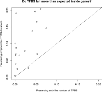
Figure 1: Scatter plot of $p$-values for the same test under two different null models.

4.2 Deciding What Should Be Preserved in the Null Model: Randomizing Genes Instead of Transcription Factors Binding Sites

In this section there are two pairs of null models with preservation ordering according to case A in Section 3. The $p$-values are ordered as expected: more preservation gives larger $p$-values.

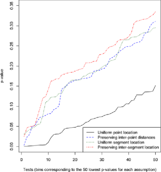
Figure 2: Empirical cumulative distribution of $p$-values under four different null models. The different null models correspond to whether TFBS or genes are randomized, and whether the empirical inter-element distances are preserved or not.

In the above discussion, we have implicitly assumed that the TFBS distribution should be stochastic in the null model, while genes are preserved exactly at their genomic locations. This seems reasonable from a biological standpoint, as the location of binding sites can generally be assumed to follow the location of genes chronologically through evolution (although there may be exceptions, such as coding regions copied into genomic regions that already have an established regulatory machinery). However, one should also consider which of the tracks have the more complex structure. This structure should be preserved in the null model, and one would prefer to randomize the track with the simplest structure. Although the location of genes is clearly not uniform, it can be argued that the TFBS has an even more complex structure. The reason is that individual TFBS fall as clusters with specific intra-cluster structure inside regulatory regions, with regulatory regions again having a certain structure in relation to genes. Indeed, as can be seen from Figure 2, the $p$-values are somewhat higher when randomizing genes as opposed to TFBS. In the figure we compare the two null models described above randomizing TFBS-positions and two null models where we randomize the gene locations with random positioning and preserving inter-gene distances. These two null models, randomizing the gene locations, are also examples of case A in Section 3. As expected, the second null model gives larger $p$-values. The two models with gene randomization also give larger $p$-values than the two models with TFBS randomization, indicating that the models with gene randomization preserve more of the complex interaction between genes and TFBS than the two other models. Note also that the difference between the two models randomizing genes is smaller than between the two models randomizing TFBS. This indicates that preserving inter-distances is more important for TFBS than for genes.

5 Significance Ordering for Data That Display Internal Clustering: Transcription Factor Binding and Chromatin States

In this section we will show that clustering is present in a large amount of genomic tracks. Clustering leads to the preservation ordering shown in case B of Section 3. Again, the $p$-values are ordered, with more preservation giving larger $p$-values.

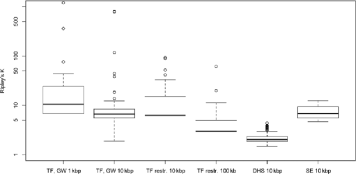
Figure 3: Box plot of scaled Ripley’s $K$ values for several collections of ENCODE and RoadMap Epigenomics tracks. The two left boxes are based on 81 TF ChIP-seq tracks with genome wide data, followed by two boxes with the same data but restricted to selected regions of size $>100$ kb that are more than 100 kbps away from the nearest gene, followed by a box based on 147 tracks of DHS for different cell types and finally a box with elements of chromatin state “5-Strong Enhancer” in nine different cell types. The clustering is analyzed for two different scales for the two first data types.

The DNA has to be highly compacted in order to fit into a cell. At the same time, it has to be accessible, for example, to the binding of transcription factors in order to allow efficient gene regulation. To achieve controlled compactness and accessibility, DNA is packed in a structured manner at multiple levels. The first such organizational layer consists of the DNA double helix, at the order of 100 base pairs, wound around small protein complexes called nucleosomes (Kornberg and Lorch, 1999). These nucleosomes can be modified through the attachment of other molecules to the proteins of the nucleosomes, which are called histones. This is referred to as histone modification, and serves a regulatory role in itself (Cairns, 2009). Recently, it has become possible to create genome-wide maps of histone modifications through the use of high-throughput sequencing protocols (Wang et al., 2008). It has been suggested that combinations of such histone modifications in a given region, referred to as chromatin states, can be used as a mark of the functional role of the region (Ernst et al., 2011). One of the proposed chromatin states, the “5-enhancer” (shortened to “SE” in part of the following text), is suggested to correspond to regions that play a role in gene regulation by providing accessible binding sites to several transcription factors. It is thus interesting to see whether different TFs indeed shows a higher than expected density of experimentally determined binding events inside these regions. To investigate this, we considered a collection of 82 tracks of experimentally determined TF binding events in blood cells (cell type gm12878) generated through the ENCODE project. The tracks are originally of type Segments, corresponding to called signal peaks of ChIP-seq experiments (Kim et al., 2005). These peak segments are around 100 bps long, reflecting experimental inaccuracy in the determination of binding sites that are themselves around 5–25 bp long (Wingender et al., 1996). The real binding sites are often, but not always, located around the center of these peak regions. In our analyses, we used the midpoints of the peak regions as binding site locations. For each TF, we then tested whether the binding locations occurred inside regions in the “5-enhancer” chromatin state more than expected by chance.

An analysis of the direct relation between TF binding locations and chromatin states might be strongly confounded by a common relation to gene locations. To reduce this potentially confounding factor, we focused the study of the relation between TF binding and enhancer states on only contiguous regions of size $>100$ kb, that are more than 100 kbps away from the nearest gene. Parts of these regions are located in centromeres, where neither TF binding events nor chromatin states can be mapped. To avoid any bias due to this, we constrained the analysis regions to only part of the regions being located in the chromosome arms. There is a total of 580 such regions in the human genome (using the Ensembl gene definition for computing distance from genes), ranging in size from 100 kbp to 2.6 Mbp and covering a total of 151 Mbps.

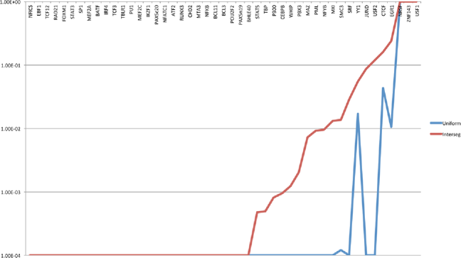
Figure 4: $p$-values for hypothesis testing of whether midpoints of ChIP-seq peaks for 47 different TF were located more than expected inside regions of the chromatin state 5-Strong Enhancer. $p$-values were computed for two different null models: random location of the midpoints or preserving the inter-point distances. The TFs on the $x$-axis were sorted according to the $p$-value achieved when preserving inter-point distances in the null model.

As can be seen from Figure 3, ENCODE tracks display a strong clustering tendency across different scales for a large number of tracks of different types. The scaled Ripley $K$ values are described in Section 3.1. All the collections show a typical clustering tendency well beyond the neutral value of 1. Based on these results, we claim that clustering is typical for genomic data of this type. We observe very few data sets where we find repulsion. Case B in Section 3 shows that clustering may give increasing $p$-values for null models: if we reduce or remove the clustering in the stochastic model, that is, reduce the preservation, then the $p$-values decrease. Hence, the $p$-value from the null models are ordered according to increasing preservation of the clustering. When testing the clustering it is important to apply a scale that is adapted to the length of the observed property, for example, TFs. The ordering of the $p$-values depends on the scale of clustering relative to the length of the properties (e.g., genes) in the other tracks used in the test.

Furthermore, we tested whether ChIP-seq peaks for 47 different TFs transcription factors were located more than expected inside regions of chromatin state 5-Strong Enhancer. $p$-values for two different null models with random location of the CHIP-seq peaks or preserving the inter-distances from the original tracks are shown in Figure 4. A total of 81 tracks of the TF ChIP-seq peak region for the cell type gm12878 were retrieved from the ENCODE data collection and analyzed against Strong Enhancer inside regions of size $>100$ kb that were more than 100 kbps away from the nearest gene. For 34 of these tracks, there were less than a total of 20 peaks across all analysis regions, and they were removed from the analysis. The $p$-values were computed based on Monte Carlo, using 10,000 samples, thus giving a minimum achievable $p$-value of 1E$-$4. For some TFs, this minimum $p$-value was achieved using either null model. For other TFs, either null model resulted in a $p$-value of 1. In all cases where the two null models resulted in different $p$-values, the null model that preserves inter-point distances gave the highest $p$-value.

As we can see from Figure 4, very low $p$-values are reached for many of the tests, confirming that the 5-Strong Enhancer chromatin state captures histone modification patterns indicative of TF binding. Indeed, when considering the union of binding locations across all TFs, the relation between TFs and SE is highly significant ($p<0.00001$) for either null model. Our interpretation of the results is that it clearly appears to be a relation of TF binding and the 5-Strong Enhancer chromatin state, but that the data limitation due to only considering regions that meets the strict criteria above does not allow a conclusion to be drawn regarding this relation for all TFs, when considering only the behavior in these regions. The systematic difference between $p$-values achieved using the two null models then reflects that the null model preserving inter-point distances more accurately portrays the possibility of concluding on the TF–SE relation, while the null model disregarding the clustering of TF points (inter-point distances) gives $p$-values that are lower than the degree of certainty that can really be assigned to the TF–SE relation in the considered analysis regions.

6 False Rejections of Null Models Using Simulated Data

In this section we perform hypothesis tests based on simulated data with a clustering representative for genomic data. One test has synthetic tracks for points and segments and another test uses real TF tracks and simulated segment tracks. We generate the tracks independently from each other, so the null hypothesis of independence should not be rejected for any of the tests. In both cases, we get many false rejections if we assume uniform locations of points, but good results when we preserve inter-point distances.

Table 1: Number of falsely rejected null hypotheses under different combinations of data generation procedures and testing assumptions. Two tracks of points and segments, respectively, are generated independently, and then tested for significant relation. The different columns correspond to whether points or segments are generated uniformly (Poisson) or with a tendency for clustering. The different rows correspond to whether points or segments are assumed to be random in the null model, as well as whether location is assumed to be uniformly distributed or according to a preserved empirical distribution of inter-element distances

	Generation
Assumption	Uniform	Clustered points	Clustered segments
Uniform point location (analytic)	0/100	17/100	0/100
Uniform point location (MC)	0/100	19/100	0/100
Preserving inter-point distances	0/100	0/100	0/100
Uniform segment location (MC)	0/100	0/100	0/100

The previously presented genomic cases confirm that a null model with a higher level of preservation typically gives higher $p$-values on real data. However, they do not tell us which null model should be preferred. As the simple null models will typically be easier to implement, will often allow computationally fast analytical solutions and will typically give more significance, they may be a tempting choice for a practitioner. However, when their assumptions are not met, there is a severe risk of false positive findings, due to the failure of the null model to account for intrinsic characteristics of the data, unrelated to the null and alternative hypotheses that are on trial.

In order to study the potential severity of false positive findings due to unrealistic null models, we performed a simulation study. Two tracks were generated independently, but with various intrinsic clustering-related properties. They were then tested for a relation under different null models. The results are shown in Table 1. The synthetic tracks were generated according to the approach described in Sandve et al. (2010). Independent points were generated according to a Poisson distribution with $\lambda=0.01$. Clustered points were generated under an intra-cluster Poisson distribution with $\lambda=0.1$ and inter-cluster Poisson with $\lambda=0.01$, with each point having a probability $0.3$ of forming a new cluster. Segments were generated similarly to points, with distance between consecutive segments following a Poisson distribution with $\lambda=0.01$. Lengths of segments were distributed uniformly between $10$ and $100$ base pairs. For each combination, 100 separate tests were performed and the number of false rejections reported after multiple testing correction at 20% FDR. We notice that inappropriate assumptions could lead to up to 19% of null hypotheses being falsely rejected after correction for multiple testing.

Preserving more of the individual properties (inter-element distances) was the safe choice, essentially avoiding false rejections, while assuming uniform point locations resulted in a high degree of false rejections, whether the test was resolved analytically or by Monte Carlo simulation. For this particular test, using a too simple assumption on segment location (assuming uniform location for segments that were in reality clustered) presented less of a problem. The reason for this is that the autocorrelation between values of $X_{i}$, as discussed in Section 3, would be relatively low, and thus not lead to any strong underestimation of $p$-values.

It was shown in the previous two sections that using simple null models led to lower $p$-values and more rejections when testing the relation of TF binding to genes to certain chromatin states. Although it would be tempting to consider the higher significance as a sign of better power of the testing setup, the assumption of uniform TF binding location is problematic and could lead to $p$-values being underestimated. We have also shown on purely simulated data that too simple and unrealistic assumptions can lead to a high degree of false rejections. Here, we combine the real data of TF binding with simulated segment data having the same characteristics as genes and chromatin states, but where the simulated data is generated independently from TF binding locations and chromatin states. The null hypothesis should then not be rejected in any test after multiple testing correction.

For each chromosome band with at least 5 MitF binding sites, we tested whether these binding sites occur differently than expected inside simulated segments. This resulted in $H_{0}$ being rejected in 1 out of 73 bins at 10% FDR when assuming uniform MitF locations. However, when performing the tests only on 14 bins with a more satisfactory amount of data (at least 10 MitF binding sites), the null hypothesis is rejected in 4 out of 14 bins (still at 10% FDR). This high rate of false rejections suggests that part of the significance observed for MitF versus genes or chromatin states under the assumption of uniform location is likely due to underestimation of $p$-values due to the inadequacy of this null model. Conversely, preserving the empirical distribution of inter-MitF distances leads to no rejections of $H_{0}$ at 10% FDR, either when testing in all 73 bins or in the 14 bins with most MitF binding sites. This suggests that the preservation of inter-point distances is able to capture the intrinsic structure of the MitF track in an appropriate manner.

In summary, we find that the choice of null model strongly influences the results. Mainly, the difference is that a null model preserving more of the observed data yields higher $p$-values. Tests on simulated data show that an overly simple null model, preserving too little of the observed data, can lead to a large number of false rejections, even after correcting for multiple testing.

7 Discussion

In this paper we have studied the choice of Monte Carlo null models. We have defined the Monte Carlo state space as the (finite) set of allowed resamplings of the observed data, and defined a Monte Carlo null model preservation hierarchy. We have discussed the null complexity principle, namely, that an ordering of preservation may imply a corresponding ordering of statistical significance (i.e., of estimated $p$-values), and illustrated the use of our result on real data sets of general interest.

The choice of null model is very application dependent, so it is difficult to give general guidelines. However, two general approaches are as follows: (1) to be conservative and choose the largest $p$-value and (2) use the most restricted null model (which, however, should still have sufficient freedom of variability to provide an efficient test), so that we are “close to the truth,” that is, faithful to restriction given by the phenomenon under study. Because of the null complexity principle, approaches (1) and (2) will usually coincide.

A fundamental feature of the Monte Carlo approach to statistical inference is that conclusions may only be drawn regarding the actual observed data. In other words, there is no prospect for generalizations to any (hypothetical or real) population. While some may see this as a serious drawback of Monte Carlo methods, we feel that this line of objection to randomization methodology is often quite misguided. Obviously, the idea of random sampling from a population is both useful and extremely entrenched in classical statistics. However, often is it very hard to even conceive of the “population” in which random sampling is supposed to take place. Genomics and DNA sequences are good examples of this. In many cases, the Monte Carlo method is simply a more natural approach: we do not wish to draw conclusions from a sample to a population, it is really the (single, unique) sample itself that we are genuinely interested in. In this paper we have focused on examples from genetics since this is our main interest and motivation for the paper. But similar problems are encountered in other areas such as ecology, as documented in a separate report; see Ferkingstad, Holden and Sandve (2013).

An interesting topic for future work would be to study the implications for the multiple hypothesis testing setting. For a discussion of some computational and conceptual challenges of Monte Carlo multiple testing, see Sandve, Ferkingstad and Nygård (2011). The multiple testing problem is particularly important in genomics, but it also appears in ecology; see, for example, Gotelli and Ulrich (2010).

Our main focus has been avoiding false positives due to too simple null models. Of course, false negatives also occur, and the effect of differing null models on the power of tests should be further studied. In order to avoid underpowered tests, a very general advice is the following. Most test statistics in the paper are based on counting, hence, the variance of test statistics decreases as $1/N$ where $N$ is the number of samples. But observations may be correlated, reducing power. We may have very high correlation between a large number of observations. It is important to be aware of this and try to find test statistics where the correlation between observations is as small as possible.

Finally, we have also considered a third type of null model preservation, where the data is a sequence of categorical variables, for example, …ACGT…for a DNA sequence. The distribution for each variable depends on the value of the previous $n$ variables. In this model, it is possible to have the same probability distribution for sequences of length $n$ as in the observed data. Then, increasing $n$ implies preservering more of the probabilistic structure of the original data. We omitted this material to make the paper shorter and more focused. A separate paper on this topic is in preparation.

References

- Benjamini and Hochberg (1995) {barticle}[mr] \bauthor\bsnmBenjamini, \bfnmYoav\binitsY. and \bauthor\bsnmHochberg, \bfnmYosef\binitsY. (\byear1995). \btitleControlling the false discovery rate: A practical and powerful approach to multiple testing. \bjournalJ. Roy. Statist. Soc. Ser. B \bvolume57 \bpages289–300. \bidissn=0035-9246, mr=1325392 \bptokimsref\endbibitem
- Berman et al. (2002) {barticle}[pbm] \bauthor\bsnmBerman, \bfnmBenjamin P.\binitsB. P., \bauthor\bsnmNibu, \bfnmYutaka\binitsY., \bauthor\bsnmPfeiffer, \bfnmBarret D.\binitsB. D., \bauthor\bsnmTomancak, \bfnmPavel\binitsP., \bauthor\bsnmCelniker, \bfnmSusan E.\binitsS. E., \bauthor\bsnmLevine, \bfnmMichael\binitsM., \bauthor\bsnmRubin, \bfnmGerald M.\binitsG. M. and \bauthor\bsnmEisen, \bfnmMichael B.\binitsM. B. (\byear2002). \btitleExploiting transcription factor binding site clustering to identify cis-regulatory modules involved in pattern formation in the Drosophila genome. \bjournalProc. Natl. Acad. Sci. USA \bvolume99 \bpages757–762. \biddoi=10.1073/pnas.231608898, issn=0027-8424, pii=99/2/757, pmcid=117378, pmid=11805330 \bptokimsref\endbibitem
- Bickel et al. (2010) {barticle}[mr] \bauthor\bsnmBickel, \bfnmPeter J.\binitsP. J., \bauthor\bsnmBoley, \bfnmNathan\binitsN., \bauthor\bsnmBrown, \bfnmJames B.\binitsJ. B., \bauthor\bsnmHuang, \bfnmHaiyan\binitsH. and \bauthor\bsnmZhang, \bfnmNancy R.\binitsN. R. (\byear2010). \btitleSubsampling methods for genomic inference. \bjournalAnn. Appl. Stat. \bvolume4 \bpages1660–1697. \biddoi=10.1214/10-AOAS363, issn=1932-6157, mr=2829932 \bptokimsref\endbibitem
- Cairns (2009) {barticle}[pbm] \bauthor\bsnmCairns, \bfnmBradley R.\binitsB. R. (\byear2009). \btitleThe logic of chromatin architecture and remodelling at promoters. \bjournalNature \bvolume461 \bpages193–198. \biddoi=10.1038/nature08450, issn=1476-4687, pii=nature08450, pmid=19741699 \bptokimsref\endbibitem
- Efron (2004) {barticle}[mr] \bauthor\bsnmEfron, \bfnmBradley\binitsB. (\byear2004). \btitleLarge-scale simultaneous hypothesis testing: The choice of a null hypothesis. \bjournalJ. Amer. Statist. Assoc. \bvolume99 \bpages96–104. \biddoi=10.1198/016214504000000089, issn=0162-1459, mr=2054289 \bptokimsref\endbibitem
- Ernst et al. (2011) {barticle}[author] \bauthor\bsnmErnst, \bfnmJason\binitsJ., \bauthor\bsnmKheradpour, \bfnmPouya\binitsP., \bauthor\bsnmMikkelsen, \bfnmTarjei S.\binitsT. S., \bauthor\bsnmShoresh, \bfnmNoam\binitsN., \bauthor\bsnmWard, \bfnmLucas D.\binitsL. D., \bauthor\bsnmEpstein, \bfnmCharles B.\binitsC. B., \bauthor\bsnmZhang, \bfnmXiaolan\binitsX., \bauthor\bsnmWang, \bfnmLi\binitsL., \bauthor\bsnmIssner, \bfnmRobbyn\binitsR., \bauthor\bsnmCoyne, \bfnmMichael\binitsM., \bauthor\bsnmKu, \bfnmManching\binitsM., \bauthor\bsnmDurham, \bfnmTimothy\binitsT., \bauthor\bsnmKellis, \bfnmManolis\binitsM. and \bauthor\bsnmBernstein, \bfnmBradley E.\binitsB. E. (\byear2011). \btitleMapping and analysis of chromatin state dynamics in nine human cell types. \bjournalNature \bvolume473 \bpages43–49. \bptokimsref\endbibitem
-
Ferkingstad, Holden and
Sandve (2013)
{bmisc}[author]
\bauthor\bsnmFerkingstad, \bfnmEgil\binitsE.,
\bauthor\bsnmHolden, \bfnmLars\binitsL. and \bauthor\bsnmSandve, \bfnmGeir Kjetil\binitsG. K.
(\byear2013).
\bhowpublishedMonte Carlo null models in ecology.
Technical Report SAMBA/20/13,
Norwegian Computing Center.
Available at \surlhttp://publications.nr.no/1370000051/
NullModelsEcology-Ferkingstad.pdf. \bptokimsref\endbibitem - Fisher (1935) {bbook}[author] \bauthor\bsnmFisher, \bfnmR. A.\binitsR. A. (\byear1935). \btitleThe Design of Experiments. \bpublisherOliver & Boyd, \blocationLondon. \bptokimsref\endbibitem
- Flicek et al. (2012) {barticle}[pbm] \bauthor\bsnmFlicek, \bfnmPaul\binitsP., \bauthor\bsnmAmode, \bfnmM. Ridwan\binitsM. R., \bauthor\bsnmBarrell, \bfnmDaniel\binitsD., \bauthor\bsnmBeal, \bfnmKathryn\binitsK., \bauthor\bsnmBrent, \bfnmSimon\binitsS., \bauthor\bsnmCarvalho-Silva, \bfnmDenise\binitsD., \bauthor\bsnmClapham, \bfnmPeter\binitsP., \bauthor\bsnmCoates, \bfnmGuy\binitsG., \bauthor\bsnmFairley, \bfnmSusan\binitsS., \bauthor\bsnmFitzgerald, \bfnmStephen\binitsS., \bauthor\bsnmGil, \bfnmLaurent\binitsL., \bauthor\bsnmGordon, \bfnmLeo\binitsL., \bauthor\bsnmHendrix, \bfnmMaurice\binitsM., \bauthor\bsnmHourlier, \bfnmThibaut\binitsT., \bauthor\bsnmJohnson, \bfnmNathan\binitsN., \bauthor\bsnmKähäri, \bfnmAndreas K.\binitsA. K., \bauthor\bsnmKeefe, \bfnmDamian\binitsD., \bauthor\bsnmKeenan, \bfnmStephen\binitsS., \bauthor\bsnmKinsella, \bfnmRhoda\binitsR., \bauthor\bsnmKomorowska, \bfnmMonika\binitsM., \bauthor\bsnmKoscielny, \bfnmGautier\binitsG., \bauthor\bsnmKulesha, \bfnmEugene\binitsE., \bauthor\bsnmLarsson, \bfnmPontus\binitsP., \bauthor\bsnmLongden, \bfnmIan\binitsI., \bauthor\bsnmMcLaren, \bfnmWilliam\binitsW., \bauthor\bsnmMuffato, \bfnmMatthieu\binitsM., \bauthor\bsnmOverduin, \bfnmBert\binitsB., \bauthor\bsnmPignatelli, \bfnmMiguel\binitsM., \bauthor\bsnmPritchard, \bfnmBethan\binitsB., \bauthor\bsnmRiat, \bfnmHarpreet Singh\binitsH. S., \bauthor\bsnmRitchie, \bfnmGraham R. S.\binitsG. R. S., \bauthor\bsnmRuffier, \bfnmMagali\binitsM., \bauthor\bsnmSchuster, \bfnmMichael\binitsM., \bauthor\bsnmSobral, \bfnmDaniel\binitsD., \bauthor\bsnmTang, \bfnmY. Amy\binitsY. A., \bauthor\bsnmTaylor, \bfnmKieron\binitsK., \bauthor\bsnmTrevanion, \bfnmStephen\binitsS., \bauthor\bsnmVandrovcova, \bfnmJana\binitsJ., \bauthor\bsnmWhite, \bfnmSimon\binitsS., \bauthor\bsnmWilson, \bfnmMark\binitsM., \bauthor\bsnmWilder, \bfnmSteven P.\binitsS. P., \bauthor\bsnmAken, \bfnmBronwen L.\binitsB. L., \bauthor\bsnmBirney, \bfnmEwan\binitsE., \bauthor\bsnmCunningham, \bfnmFiona\binitsF., \bauthor\bsnmDunham, \bfnmIan\binitsI., \bauthor\bsnmDurbin, \bfnmRichard\binitsR., \bauthor\bsnmFernández-Suarez, \bfnmXosé M.\binitsX. M., \bauthor\bsnmHarrow, \bfnmJennifer\binitsJ., \bauthor\bsnmHerrero, \bfnmJavier\binitsJ., \bauthor\bsnmHubbard, \bfnmTim J. P.\binitsT. J. P., \bauthor\bsnmParker, \bfnmAnne\binitsA., \bauthor\bsnmProctor, \bfnmGlenn\binitsG., \bauthor\bsnmSpudich, \bfnmGiulietta\binitsG., \bauthor\bsnmVogel, \bfnmJan\binitsJ., \bauthor\bsnmYates, \bfnmAndy\binitsA., \bauthor\bsnmZadissa, \bfnmAmonida\binitsA. and \bauthor\bsnmSearle, \bfnmStephen M. J.\binitsS. M. J. (\byear2012). \btitleEnsembl 2012. \bjournalNucleic Acids Res. \bvolume40 \bpagesD84–D90. \biddoi=10.1093/nar/gkr991, issn=1362-4962, pii=gkr991, pmcid=3245178, pmid=22086963 \bptokimsref\endbibitem
- Fortin and Jacquez (2000) {barticle}[author] \bauthor\bsnmFortin, \bfnmM. J.\binitsM. J. and \bauthor\bsnmJacquez, \bfnmG. M.\binitsG. M. (\byear2000). \btitleRandomization tests and spatially auto-correlated data. \bjournalBulletin of the Ecological Society of America \bvolume81 \bpages201–205. \bptokimsref\endbibitem
- Gionis et al. (2007) {barticle}[author] \bauthor\bsnmGionis, \bfnmA.\binitsA., \bauthor\bsnmMannila, \bfnmH.\binitsH., \bauthor\bsnmMielikäinen, \bfnmT.\binitsT. and \bauthor\bsnmTsaparas, \bfnmP.\binitsP. (\byear2007). \btitleAssessing data mining results via swap randomization. \bjournalACM Transactions on Knowledge Discovery from Data \bvolume1 \bpages14. \bptokimsref\endbibitem
- Goecks et al. (2010) {barticle}[pbm] \bauthor\bsnmGoecks, \bfnmJeremy\binitsJ., \bauthor\bsnmNekrutenko, \bfnmAnton\binitsA., \bauthor\bsnmTaylor, \bfnmJames\binitsJ. and \bauthor\bsnmGalaxy Team (\byear2010). \btitleGalaxy: A comprehensive approach for supporting accessible, reproducible, and transparent computational research in the life sciences. \bjournalGenome Biol. \bvolume11 \bpagesR86. \biddoi=10.1186/gb-2010-11-8-r86, issn=1465-6914, pii=gb-2010-11-8-r86, pmcid=2945788, pmid=20738864 \bptokimsref\endbibitem
- Goodman and Greenland (2007) {bmisc}[author] \bauthor\bsnmGoodman, \bfnmS.\binitsS. and \bauthor\bsnmGreenland, \bfnmS.\binitsS. (\byear2007). \bhowpublishedAssessing the unreliability of the medical literature: A response to “Why most published research findings are false.” Working Paper 135, Dept. Biostatistics, Johns Hopkins Univ., Baltimore, MD. Available at http://www.bepress.com/jhubiostat/paper135. \bptokimsref\endbibitem
- Gotelli (2000) {barticle}[author] \bauthor\bsnmGotelli, \bfnmN. J.\binitsN. J. (\byear2000). \btitleNull model analysis of species co-occurrence patterns. \bjournalEcology \bvolume81 \bpages2606–2621. \bptokimsref\endbibitem
- Gotelli and Graves (1996) {bbook}[author] \bauthor\bsnmGotelli, \bfnmN. J.\binitsN. J. and \bauthor\bsnmGraves, \bfnmG. R.\binitsG. R. (\byear1996). \btitleNull Models in Ecology. \bpublisherSmithsonian Institution, \blocationWashington, DC. \bptokimsref\endbibitem
- Gotelli and Ulrich (2010) {barticle}[pbm] \bauthor\bsnmGotelli, \bfnmNicholas J.\binitsN. J. and \bauthor\bsnmUlrich, \bfnmWerner\binitsW. (\byear2010). \btitleThe empirical Bayes approach as a tool to identify non-random species associations. \bjournalOecologia \bvolume162 \bpages463–477. \biddoi=10.1007/s00442-009-1474-y, issn=1432-1939, pmid=19826839 \bptokimsref\endbibitem
- Hanhijärvi, Garriga and Puolamäki (2009) {binproceedings}[author] \bauthor\bsnmHanhijärvi, \bfnmS.\binitsS., \bauthor\bsnmGarriga, \bfnmG.\binitsG. and \bauthor\bsnmPuolamäki, \bfnmK.\binitsK. (\byear2009). \btitleRandomization techniques for graphs. In \bbooktitleProceedings of the 9th SIAM International Conference on Data Mining (SDM’09) \bpages780–791. \bpublisherSIAM, \blocationPhiladelphia, PA. \bptokimsref\endbibitem
- Ioannidis (2005) {barticle}[pbm] \bauthor\bsnmIoannidis, \bfnmJohn P. A.\binitsJ. P. A. (\byear2005). \btitleWhy most published research findings are false. \bjournalPLoS Med. \bvolume2 \bpagese124. \biddoi=10.1371/journal.pmed.0020124, issn=1549-1676, pii=04-PLME-E-0321R2, pmcid=1182327, pmid=16060722 \bptokimsref\endbibitem
- Ioannidis et al. (2008) {barticle}[author] \bauthor\bsnmIoannidis, \bfnmJohn P A.\binitsJ. P. A., \bauthor\bsnmAllison, \bfnmDavid B.\binitsD. B., \bauthor\bsnmBall, \bfnmCatherine A.\binitsC. A., \bauthor\bsnmCoulibaly, \bfnmIssa\binitsI., \bauthor\bsnmCui, \bfnmXiangqin\binitsX., \bauthor\bsnmCulhane, \bfnmAed’in C.\binitsA. C., \bauthor\bsnmFalchi, \bfnmMario\binitsM., \bauthor\bsnmFurlanello, \bfnmCesare\binitsC., \bauthor\bsnmGame, \bfnmLaurence\binitsL., \bauthor\bsnmJurman, \bfnmGiuseppe\binitsG., \bauthor\bsnmMangion, \bfnmJon\binitsJ., \bauthor\bsnmMehta, \bfnmTapan\binitsT., \bauthor\bsnmNitzberg, \bfnmMichael\binitsM., \bauthor\bsnmPage, \bfnmGrier P.\binitsG. P., \bauthor\bsnmPetretto, \bfnmEnrico\binitsE. and \bauthor\bparticlevan \bsnmNoort, \bfnmVera\binitsV. (\byear2008). \btitleRepeatability of published microarray gene expression analyses. \bjournalNat. Genet. \bvolume41 \bpages149–155. \bptokimsref\endbibitem
- Kallio et al. (2011) {barticle}[pbm] \bauthor\bsnmKallio, \bfnmAleksi\binitsA., \bauthor\bsnmVuokko, \bfnmNiko\binitsN., \bauthor\bsnmOjala, \bfnmMarkus\binitsM., \bauthor\bsnmHaiminen, \bfnmNiina\binitsN. and \bauthor\bsnmMannila, \bfnmHeikki\binitsH. (\byear2011). \btitleRandomization techniques for assessing the significance of gene periodicity results. \bjournalBMC Bioinformatics \bvolume12 \bpages330. \biddoi=10.1186/1471-2105-12-330, issn=1471-2105, pii=1471-2105-12-330, pmcid=3199764, pmid=21827656 \bptokimsref\endbibitem
- Kell and Oliver (2004) {barticle}[pbm] \bauthor\bsnmKell, \bfnmDouglas B.\binitsD. B. and \bauthor\bsnmOliver, \bfnmStephen G.\binitsS. G. (\byear2004). \btitleHere is the evidence, now what is the hypothesis? The complementary roles of inductive and hypothesis-driven science in the post-genomic era. \bjournalBioessays \bvolume26 \bpages99–105. \biddoi=10.1002/bies.10385, issn=0265-9247, pmid=14696046 \bptokimsref\endbibitem
- Kim et al. (2005) {barticle}[author] \bauthor\bsnmKim, \bfnmTae Hoon\binitsT. H., \bauthor\bsnmBarrera, \bfnmLeah O.\binitsL. O., \bauthor\bsnmZheng, \bfnmMing\binitsM., \bauthor\bsnmQu, \bfnmChunxu\binitsC., \bauthor\bsnmSinger, \bfnmMichael A.\binitsM. A., \bauthor\bsnmRichmond, \bfnmTodd A.\binitsT. A., \bauthor\bsnmWu, \bfnmYingnian\binitsY., \bauthor\bsnmGreen, \bfnmRoland D.\binitsR. D. and \bauthor\bsnmRen, \bfnmBing\binitsB. (\byear2005). \btitleA high-resolution map of active promoters in the human genome. \bjournalNature \bvolume436 \bpages876–880. \bptokimsref\endbibitem
- Kornberg and Lorch (1999) {barticle}[pbm] \bauthor\bsnmKornberg, \bfnmR. D.\binitsR. D. and \bauthor\bsnmLorch, \bfnmY.\binitsY. (\byear1999). \btitleTwenty-five years of the nucleosome, fundamental particle of the eukaryote chromosome. \bjournalCell \bvolume98 \bpages285–294. \bidissn=0092-8674, pii=S0092-8674(00)81958-3, pmid=10458604 \bptokimsref\endbibitem
- Langaas, Lindqvist and Ferkingstad (2005) {barticle}[mr] \bauthor\bsnmLangaas, \bfnmMette\binitsM., \bauthor\bsnmLindqvist, \bfnmBo Henry\binitsB. H. and \bauthor\bsnmFerkingstad, \bfnmEgil\binitsE. (\byear2005). \btitleEstimating the proportion of true null hypotheses, with application to DNA microarray data. \bjournalJ. Roy. Statist. Soc. Ser. B \bvolume67 \bpages555–572. \biddoi=10.1111/j.1467-9868.2005.00515.x, issn=1369-7412, mr=2168204 \bptokimsref\endbibitem
- Lehmann and Romano (2005) {bbook}[mr] \bauthor\bsnmLehmann, \bfnmE. L.\binitsE. L. and \bauthor\bsnmRomano, \bfnmJoseph P.\binitsJ. P. (\byear2005). \btitleTesting Statistical Hypotheses, \bedition3rd ed. \bpublisherSpringer, New York. \bidmr=2135927 \bptokimsref\endbibitem
- Lijffijt et al. (2014) {barticle}[author] \bauthor\bsnmLijffijt, \bfnmJefrey\binitsJ., \bauthor\bsnmPapapetrou, \bfnmPanagiotis\binitsP. and \bauthor\bsnmPuolamäki, \bfnmKai\binitsK. (\byear2014). \btitleA statistical significance testing approach to mining the most informative set of patterns. \bjournalData Min. Knowl. Discov. \bvolume28 \bpages238–263. \bptokimsref\endbibitem
- Manly (2007) {bbook}[mr] \bauthor\bsnmManly, \bfnmBryan F. J.\binitsB. F. J. (\byear2007). \btitleRandomization, Bootstrap and Monte Carlo Methods in Biology, \bedition3rd ed. \bpublisherChapman & Hall/CRC, Boca Raton, FL. \bidmr=2257066 \bptokimsref\endbibitem
- Mesirov (2010) {barticle}[pbm] \bauthor\bsnmMesirov, \bfnmJill P.\binitsJ. P. (\byear2010). \btitleComputer science. Accessible reproducible research. \bjournalScience \bvolume327 \bpages415–416. \biddoi=10.1126/science.1179653, issn=1095-9203, mid=NIHMS169985, pii=327/5964/415, pmcid=3878063, pmid=20093459 \bptokimsref\endbibitem
- Noseda and McLean (2008) {barticle}[pbm] \bauthor\bsnmNoseda, \bfnmMichela\binitsM. and \bauthor\bsnmMcLean, \bfnmGary R.\binitsG. R. (\byear2008). \btitleWhere did the scientific method go? \bjournalNat. Biotechnol. \bvolume26 \bpages28–29. \biddoi=10.1038/nbt0108-28, issn=1546-1696, pii=nbt0108-28, pmid=18183010 \bptokimsref\endbibitem
- Pounds and Cheng (2006) {barticle}[pbm] \bauthor\bsnmPounds, \bfnmStan\binitsS. and \bauthor\bsnmCheng, \bfnmCheng\binitsC. (\byear2006). \btitleRobust estimation of the false discovery rate. \bjournalBioinformatics \bvolume22 \bpages1979–1987. \biddoi=10.1093/bioinformatics/btl328, issn=1367-4811, pii=btl328, pmid=16777905 \bptokimsref\endbibitem
- R Development Core Team (2011) {bmanual}[author] \bauthor\bsnmR Development Core Team (\byear2011). \btitleR: A Language and Environment for Statistical Computing. \blocationVienna, Austria. \bptokimsref\endbibitem
- Ripley (1976) {barticle}[mr] \bauthor\bsnmRipley, \bfnmB. D.\binitsB. D. (\byear1976). \btitleThe second-order analysis of stationary point processes. \bjournalJ. Appl. Probab. \bvolume13 \bpages255–266. \bidissn=0021-9002, mr=0402918 \bptokimsref\endbibitem
- Ruf et al. (2011) {barticle}[author] \bauthor\bsnmRuf, \bfnmSandra\binitsS., \bauthor\bsnmSymmons, \bfnmOrsolya\binitsO., \bauthor\bsnmUslu, \bfnmVeli Vural\binitsV. V., \bauthor\bsnmDolle, \bfnmDirk\binitsD., \bauthor\bsnmHot, \bfnmChloé\binitsC., \bauthor\bsnmEttwiller, \bfnmLaurence\binitsL. and \bauthor\bsnmSpitz, \bfnmFrançois\binitsF. (\byear2011). \btitleLarge-scale analysis of the regulatory architecture of the mouse genome with a transposon-associated sensor. \bjournalNat. Genet. \bvolume43 \bpages379–386. \bptokimsref\endbibitem
- Sandve, Ferkingstad and Nygård (2011) {barticle}[author] \bauthor\bsnmSandve, \bfnmGeir Kjetil\binitsG. K., \bauthor\bsnmFerkingstad, \bfnmEgil\binitsE. and \bauthor\bsnmNygård, \bfnmStåle\binitsS. (\byear2011). \btitleSequential Monte Carlo multiple testing. \bjournalBioinformatics \bvolume27 \bpages3235–3241. \bptokimsref\endbibitem
- Sandve et al. (2010) {barticle}[author] \bauthor\bsnmSandve, \bfnmGeir K.\binitsG. K., \bauthor\bsnmGundersen, \bfnmSveinung\binitsS., \bauthor\bsnmRydbeck, \bfnmHalfdan\binitsH., \bauthor\bsnmGlad, \bfnmIngrid K.\binitsI. K., \bauthor\bsnmHolden, \bfnmLars\binitsL., \bauthor\bsnmHolden, \bfnmMarit\binitsM., \bauthor\bsnmLiestøl, \bfnmKnut\binitsK., \bauthor\bsnmClancy, \bfnmTrevor\binitsT., \bauthor\bsnmFerkingstad, \bfnmEgil\binitsE., \bauthor\bsnmJohansen, \bfnmMorten\binitsM., \bauthor\bsnmNygaard, \bfnmVegard\binitsV., \bauthor\bsnmTøstesen, \bfnmEivind\binitsE., \bauthor\bsnmFrigessi, \bfnmArnoldo\binitsA. and \bauthor\bsnmHovig, \bfnmEivind\binitsE. (\byear2010). \btitleThe Genomic HyperBrowser: Inferential genomics at the sequence level. \bjournalGenome Biol. \bvolume11 \bnoteArticle ID R121. \bptokimsref\endbibitem
- Sandve et al. (2013a) {barticle}[author] \bauthor\bsnmSandve, \bfnmGeir K.\binitsG. K., \bauthor\bsnmGundersen, \bfnmSveinung\binitsS., \bauthor\bsnmJohansen, \bfnmMorten\binitsM., \bauthor\bsnmGlad, \bfnmIngrid K.\binitsI. K., \bauthor\bsnmGunathasan, \bfnmKrishanthi\binitsK., \bauthor\bsnmHolden, \bfnmLars\binitsL., \bauthor\bsnmHolden, \bfnmMarit\binitsM., \bauthor\bsnmLiestøl, \bfnmKnut\binitsK., \bauthor\bsnmNygård, \bfnmStåle\binitsS., \bauthor\bsnmNygaard, \bfnmVegard\binitsV., \bauthor\bsnmPaulsen, \bfnmJonas\binitsJ., \bauthor\bsnmRydbeck, \bfnmHalfdan\binitsH., \bauthor\bsnmTrengereid, \bfnmKai\binitsK., \bauthor\bsnmClancy, \bfnmTrevor\binitsT., \bauthor\bsnmDrabløs, \bfnmFinn\binitsF., \bauthor\bsnmFerkingstad, \bfnmEgil\binitsE., \bauthor\bsnmKalas, \bfnmMatús\binitsM., \bauthor\bsnmLien, \bfnmTonje\binitsT., \bauthor\bsnmRye, \bfnmMorten B.\binitsM. B., \bauthor\bsnmFrigessi, \bfnmArnoldo\binitsA. and \bauthor\bsnmHovig, \bfnmEivind\binitsE. (\byear2013a). \btitleThe Genomic HyperBrowser: An analysis web server for genome-scale data. \bjournalNucleic Acids Res. \bvolume41 \bpagesW133–W141. \bptokimsref\endbibitem
- Sandve et al. (2013b) {barticle}[pbm] \bauthor\bsnmSandve, \bfnmGeir Kjetil\binitsG. K., \bauthor\bsnmNekrutenko, \bfnmAnton\binitsA., \bauthor\bsnmTaylor, \bfnmJames\binitsJ. and \bauthor\bsnmHovig, \bfnmEivind\binitsE. (\byear2013b). \btitleTen simple rules for reproducible computational research. \bjournalPLoS Comput. Biol. \bvolume9 \bpagese1003285. \biddoi=10.1371/journal.pcbi.1003285, issn=1553-7358, pii=PCOMPBIOL-D-12-01778, pmcid=3812051, pmid=24204232 \bptokimsref\endbibitem
- Storey (2002) {barticle}[mr] \bauthor\bsnmStorey, \bfnmJohn D.\binitsJ. D. (\byear2002). \btitleA direct approach to false discovery rates. \bjournalJ. Roy. Statist. Soc. Ser. B \bvolume64 \bpages479–498. \biddoi=10.1111/1467-9868.00346, issn=1369-7412, mr=1924302 \bptokimsref\endbibitem
- Strub et al. (2011) {barticle}[pbm] \bauthor\bsnmStrub, \bfnmT.\binitsT., \bauthor\bsnmGiuliano, \bfnmS.\binitsS., \bauthor\bsnmYe, \bfnmT.\binitsT., \bauthor\bsnmBonet, \bfnmC.\binitsC., \bauthor\bsnmKeime, \bfnmC.\binitsC., \bauthor\bsnmKobi, \bfnmD.\binitsD., \bauthor\bsnmGras, \bfnmS. Le\binitsS. L., \bauthor\bsnmCormont, \bfnmM.\binitsM., \bauthor\bsnmBallotti, \bfnmR.\binitsR., \bauthor\bsnmBertolotto, \bfnmC.\binitsC. and \bauthor\bsnmDavidson, \bfnmI.\binitsI. (\byear2011). \btitleEssential role of microphthalmia transcription factor for DNA replication, mitosis and genomic stability in melanoma. \bjournalOncogene \bvolume30 \bpages2319–2332. \biddoi=10.1038/onc.2010.612, issn=1476-5594, pii=onc2010612, pmid=21258399 \bptokimsref\endbibitem
- Visel, Rubin and Pennacchio (2009) {barticle}[pbm] \bauthor\bsnmVisel, \bfnmAxel\binitsA., \bauthor\bsnmRubin, \bfnmEdward M.\binitsE. M. and \bauthor\bsnmPennacchio, \bfnmLen A.\binitsL. A. (\byear2009). \btitleGenomic views of distant-acting enhancers. \bjournalNature \bvolume461 \bpages199–205. \biddoi=10.1038/nature08451, issn=1476-4687, mid=NIHMS225119, pii=nature08451, pmcid=2923221, pmid=19741700 \bptokimsref\endbibitem
- Wang et al. (2008) {barticle}[author] \bauthor\bsnmWang, \bfnmZhibin\binitsZ., \bauthor\bsnmZang, \bfnmChongzhi\binitsC., \bauthor\bsnmRosenfeld, \bfnmJeffrey A.\binitsJ. A., \bauthor\bsnmSchones, \bfnmDustin E.\binitsD. E., \bauthor\bsnmBarski, \bfnmArtem\binitsA., \bauthor\bsnmCuddapah, \bfnmSuresh\binitsS., \bauthor\bsnmCui, \bfnmKairong\binitsK., \bauthor\bsnmRoh, \bfnmTae-Young\binitsT.-Y., \bauthor\bsnmPeng, \bfnmWeiqun\binitsW., \bauthor\bsnmZhang, \bfnmMichael Q.\binitsM. Q. and \bauthor\bsnmZhao, \bfnmKeji\binitsK. (\byear2008). \btitleCombinatorial patterns of histone acetylations and methylations in the human genome. \bjournalNat. Genet. \bvolume40 \bpages897–903. \bptokimsref\endbibitem
- Wingender et al. (1996) {barticle}[author] \bauthor\bsnmWingender, \bfnmEdgar\binitsE., \bauthor\bsnmDietze, \bfnmPeter\binitsP., \bauthor\bsnmKaras, \bfnmHolger\binitsH. and \bauthor\bsnmKnüppel, \bfnmR.\binitsR. (\byear1996). \btitleTRANSFAC: A database on transcription factors and their DNA binding sites. \bjournalNucleic Acids Res. \bvolume24 \bpages238–241. \bptokimsref\endbibitem
- Zhou and Wong (2004) {barticle}[pbm] \bauthor\bsnmZhou, \bfnmQing\binitsQ. and \bauthor\bsnmWong, \bfnmWing H.\binitsW. H. (\byear2004). \btitleCisModule: De novo discovery of cis-regulatory modules by hierarchical mixture modeling. \bjournalProc. Natl. Acad. Sci. USA \bvolume101 \bpages12114–12119. \biddoi=10.1073/pnas.0402858101, issn=0027-8424, pii=0402858101, pmcid=514443, pmid=15297614 \bptokimsref\endbibitem