A Parametric Framework for the Comparison of Methods of Very Robust Regression

Abstract

There are several methods for obtaining very robust estimates of regression parameters that asymptotically resist 50% of outliers in the data. Differences in the behaviour of these algorithms depend on the distance between the regression data and the outliers. We introduce a parameter $\lambda$ that defines a parametric path in the space of models and enables us to study, in a systematic way, the properties of estimators as the groups of data move from being far apart to close together. We examine, as a function of $\lambda$, the variance and squared bias of five estimators and we also consider their power when used in the detection of outliers. This systematic approach provides tools for gaining knowledge and better understanding of the properties of robust estimators.

, and

1 Introduction

Multiple regression is one of the main tools of applied statistics. It has, however, long been appreciated that ordinary least squares as a method of fitting regression models is exceptionally susceptible to the presence of outliers. Instead, very robust methods, that asymptotically resist 50% of outliers, are to be preferred. Our paper presents a systematic, parameterised framework for the nonasymptotic comparison of these methods.

Very robust regression was introduced by Rousseeuw (1984) who developed suggestions of Hampel (1975) that led to the Least Median of Squares (LMS) and Least Trimmed Squares (LTS) algorithms. For some history of more recent developments see Rousseeuw and Van Driessen (2006). More general discussions of robust methods are in Maronna, Martin and Yohai (2006) and Morgenthaler (2007). We illustrate our methods for the comparison of high-breakdown regression procedures with comparisons of the performance of LTS and other well-established methods, including S and MM estimators, with that of a publicly available algorithm for very robust regression that uses the Forward Search (FS). See Atkinson, Riani and Cerioli (2010) for a recent discussion of the FS.

Very robust regression estimators share the property that, asymptotically, they have a breakdown point of 50% (see Section 3.2) as the main data and outliers become infinitely far apart. In order to distinguish between the estimators we study, in a systematic way, their properties as the distance between the two groups of observations decreases. In Section 4 we introduce a parameterised framework, with parameter $\lambda$, for moving the outliers along a trajectory which is initially remote from the main data, but which then passes close to it before again becoming far away. We control whether, at their closest, the two populations share the same centre. We design measures of overlap to calibrate the trajectories.

Numerical results are in Sections 5 and 6. In Section 5 we take the outliers from the regression model to have a multivariate normal distribution. This provides a very general scenario for outliers that can range from a seemingly random scatter around the regression plane to points virtually on a line. The special case of point contamination is explored in Section 6. Boxplots of the estimates from the five methods as $\lambda$ varies indeed show that, for wide separations, the methods have similar properties. However, they differ markedly as the two populations converge. In order to summarise this information, we look at cumulative plots, over the range of $\lambda$, of the variance and squared bias of the estimators. Another method of comparing robust estimators is by their properties for outlier detection (Cook and Hawkins (1990)). In Section 5 we calculate power curves as a function of $\lambda$ for the number of outliers detected. Since the curves indicate that the estimators provide tests of varying sizes, we find the size of the outlier tests in Section 7.

There are two main conclusions. The first is that the parameterised family of departures provides a cogent framework for investigating the behaviour of very robust estimators. The second is that we can clearly establish the properties of the various methods of very robust regression in terms of the bias and variance of estimators and the size and power of outlier tests.

The approach is motivated in the next section by an example in which there is a mixture of two regression lines. Such data arise in the analysis of trade where different countries or suppliers may report different relationships between value and quantity. Although, in our example, there are only two countries, which makes the data appropriate for a robust analysis assuming one model describes at least half the data, there is no reason why there should not be several suppliers. The comparative robust analysis of the data is in Section 8.

2 An Example: Trade Data

Our interest in the behaviour of robust regression procedures when the main data and outliers are close together was stimulated by a seemingly simple example with a single explanatory variable. The data, shown in Figure 1, are of a kind discussed by Perrotta, Riani and Torti (2009) in the detection of fraud in international trade, where false declarations of price are used in tax evasion and money laundering. The result is data which are a mixture of regression lines.

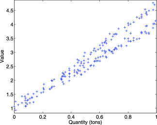
Figure 1: Trade data: A mixture of two regression lines.

There are 180 observations in Figure 1 that come from two firms. The structure is of two lines that overlap for lower values; any kind of separation is likely to be impossible. However, the two lines are clearly separate for the higher values of $y$ and $x$ and a robust procedure should respond to this pattern, by downweighting some of the observations in estimation and flagging them as outliers. If the outlier pattern suggests that there is a mixture of regression models, the analysis can move to clusters of regression lines, as in García-Escudero et al. (2010). But the first stage is the identification of outliers, for which a robust fit is required. Interest in the analysis is not in individual outliers but whether the two lines differ. Accordingly, in Section 4 we introduce a Bonferroni adjustment to provide, at least theoretically, the desired samplewise size of the outlier test. We return to the analysis of these data in Section 8.

3 Models, Data, Robustness and Methods

3.1 Outliers and Regression

We consider the usual regression model with random carriers [Huber and Ronchetti (2009), page 197]. The observations are i.i.d. random vectors ($y$, $x^{T})\in\Re^{p+1}$, where $y\in\Re$ and $x\in\Re^{p}$ satisfy

$$y=x^{T}\beta+u.$$ (1)

The random errors $u$ are distributed independently of the covariates $x$ and $\beta$ is the $p\times 1$ vector parameter of interest.

In the absence of outliers the least squares estimate $\hat{\beta}$ is the best linear unbiased estimator of $\beta$. However, even a single outlier can cause $\hat{\beta}$ to be severely biased. Figure 2 of Rousseeuw (1984) is a paradigmatic example in which a cluster of 20 outliers at a remote point in $X$-space cause the least squares fitted line to pass close to the cluster. The robust line, in that case LMS, completely downweights the outliers and is close to the least squares line for the 30 remaining data points when the outliers have been deleted.

Of course, the outliers are not usually known and the problems of robust estimation and outlier detection are closely related. In robust estimation a fit is found which is close to that without the outliers. The robust fit then allows identification of all important outliers. However, the outliers may be difficult to identify from a nonrobust fit since their inclusion can seriously bias the parameter estimates and make the outliers seem less remote. “Backward” methods of outlier detection that start from a fit to all data and then proceed by eliminating observations that appear to be outlying can therefore fail.

One example for regression is a synthetic data set due to Hawkins, Bradu and Kass (1984) with $n=75$ and three explanatory variables. The figures on page 95 of Rousseeuw and Leroy (1987) show that the least squares residuals, unlike those from LMS, are not sufficiently large to call attention to the ten outlying observations. Numerous other examples for regression are in Chapters 3 and 4 of Atkinson and Riani (2000); further plots for the Hawkins, Bradu and Kass (1984) data are on pages 72 and 73.

3.2 Maxbias and Breakdown Point

Robustness is concerned with fitting a single model to data which are generated by two, or maybe more, models. We suppose that the larger part of the data, $1-\varepsilon$, where $0<\varepsilon<0.5$, is generated by the model $M_{1}(\theta_{1})$ and the remaining part $\varepsilon$ of the data is generated by the model $M_{2}(\theta_{2})$. In the absence of outliers, that is, when $\varepsilon=0$, an ideal robust estimator would have a variance that achieved the Cramer–Rao lower bound. If the data were contaminated, the estimate would be unbiased. Such estimators do not exist. Maronna, Martin and Yohai [(2006), Section 3.4] describe some compromises between the two properties.

Robust methods study the properties of methods that fit $M_{1}(\theta_{1})$ in ignorance of knowledge of the form of the outlier generating model $M_{2}(\theta_{2})$, which can be quite general. When $M_{1}(\cdot)$ is a regression model, $M_{2}(\cdot)$ is often taken, for example, to distribute observations randomly over a large space, concentrate them in a cluster or to be a second regression model. There is no difficulty in having $M_{1}(\theta)=M_{2}(\theta)$, but then we must have $\theta_{1}\neq\theta_{2}$.

With $M_{1}(\theta_{1})$ the usual regression model (1), let $\mathrm{E}u^{2}=\sigma^{2}<\infty$ and $I(x)=\mathrm{E}xx^{T}$. The bias of an estimator $\hat{\beta}$ of $\beta$ is

$$b(\hat{\beta})=\bigl{\{}(\hat{\beta}-\beta)^{T}I(x)(\hat{\beta}-\beta)\bigr{\}}^{0.5}.$$ (2)

The bias depends on the estimator, the distribution of $y$ and $x$, the amount of contamination $\varepsilon$ and on $M_{2}(\theta_{2})$. In the robustness literature dependence on $M_{2}(\theta_{2})$ is removed by considering estimators that minimise the maximum (asymptotic) bias within a particular class of estimators. The maxbias curve shows how the maximum bias varies with $\varepsilon$. The breakdown point of an estimator is the minimum value of $\varepsilon$ for which $b(\hat{\beta})$ in (2) equals $\infty$. The estimators we consider all have an asymptotic breakdown point of 50%. An introduction to these ideas for regression is given by Maronna, Martin and Yohai [(2006), Section 5.9]. Although 50% is customarily considered to be the maximum possible breakdown value, higher values may occur in clustering.

Unfortunately maxbias curves are only calculable for some estimators and distributions of $x$. The latter are often assumed to be elliptically symmetrical. A summary of the literature is given by Berrendero and Zamar (2001) who extend results on maxbias curves to regression models with intercepts and to regressors that have Student’s $t$ and Cauchy distributions, although without intercepts. Berrendero, Mendes and Tyler (2007) find maxbias curves for MM estimators, again without intercepts. We describe MM estimators in Section 3.3.

The theoretical results that are available are asymptotic and do not cover all estimators or models of interest to us. A few numerical results are available for finite samples. Figure 5.14 of Maronna, Martin and Yohai (2006) plots biases of several estimators as a function of a single parameter, the slope of the regression line for the contaminating observations. Figure 3 of García-Escudero et al. (2010) is more in the spirit of our numerical approach. It shows the simulated bias as a point cluster of outliers moves around a regression line. When the outliers are very close to the line, the bias is negligible, as it is when the outliers are far away and are easily downweighted by, in this case, LTS. Only for intermediate outliers is the bias appreciable.

In our numerical comparisons we study the variance as well as the bias of the estimators. In addition, following the comments in Section 3.1 about the relationship between robustness and outlier detection, we asses the power of outlier tests using residuals from robustly fitted models.

3.3 Five Methods for Very Robust Regression

We compare and contrast the properties of what are currently considered the five best methods for very robust regression. The algorithms that we use are all publicly available from the Forward Search Data Analysis (FSDA) Matlab toolbox. See Riani, Perrotta and Torti (2012). In this section we outline the methods that we compare. Full implementation details of the algorithms are in the documentation of the FSDA library. Numerically, all algorithms involve selecting many subsets from the data. An important factor in our ability to conduct as many simulations as were necessary is the efficient sampling of subsets provided in FSDA as described by Torti et al. (2012).

Traditional robust estimators attempt to limit the influence of outliers by replacing the squares of the residuals in least squares estimation of $\beta$ by a function $\rho$ of the residuals which is bounded. Of the numerous forms that have been suggested for $\rho(\cdot)$ (Andrews et al. (1972); Hampel et al. (1986); Huber and Ronchetti (2009)), we use the most popular choice, Tukey’s Biweight, in which extreme residuals are replaced by the value $c^{2}/6$. See, for example, Rousseeuw and Leroy (1987), (4.31). The M-estimator of scale $\tilde{\sigma}_{M}$ is the solution to a second equation, for example, Rousseeuw and Leroy (1987), (4.30), depending on a second $\rho$ function and a constant $K_{c}$. Although the two $\rho$ functions may be different, we again use the biweight. The minimum value of $\tilde{\sigma}_{M}$ which satisfies this second equation provides the S-estimate of scale ($\tilde{\sigma}_{S}$) with associated estimate of the vector of regression coefficients ($\tilde{\beta}_{S}$). $K_{c}$ and $c$ are related constants which are linked to the breakdown point of the estimator of $\beta$. Fixing the breakdown point at 50% gives a value for 1.547 for $c$ and an efficiency for estimation of 28.7% [Rousseeuw and Leroy (1987), pages 135–143].

The MM-regression estimator is intended to improve the S estimator. The S estimate of scale $\tilde{\sigma}_{S}$ is used and kept fixed to estimate $\beta$, but with a value of $K_{c}$ giving a higher efficiency. Because of the relationship between $K_{c}$ and $c$, the hope expressed by Rousseeuw and Leroy [(1987), page 143] is that the MM estimator maintains its high breakdown point for finite samples. Following the recommendation of Maronna, Martin and Yohai [(2006), page 126], we take $K_{c}$ such that the (asymptotic) nominal efficiency is 85%, which gave a high-breakdown estimator in our examples, which included up to 23% of outliers. Small numerical experiments indicate that even slight increases, for example, to a nominal efficiency of 87%, result in very low breakdown and estimates similar to those from least squares.

The remaining three estimators of $\beta$ result from more direct approaches. The forward search (FS) uses least squares to fit subsets of observations of increasing size $m$ to the data, with $p\leq m\leq n$. The forward search for regression was introduced by Atkinson and Riani (2000). A recent general review of forward search methods is Atkinson, Riani and Cerioli (2010). For efficient parameter estimation $m$ should increase until all $n-m$ observations not in the subset used for fitting are outliers. The outliers are found by testing at each step of the search. The effect of simultaneous testing can be severe (Atkinson and Riani (2006)); the FS algorithm is designed to have size $\alpha$ of declaring an outlier free sample to contain at least one outlier. We perform the outlier test for individual observations at a Bonferronised size $\alpha^{*}=\alpha/n$, so taking the $1-\alpha^{*}$ cutoff value of the reference distribution. In our calculations $\alpha=0.01$. The automatic algorithm is based on that of Riani, Atkinson and Cerioli (2009) who used scaled Mahalanobis distances to detect outliers in multivariate normal data. For regression we replace these distances by deletion residuals.

In Least Trimmed Squares (LTS) [Rousseeuw (1984), page 876] the search is over subsets of size $h$ for which the residual sum of squares from least squares estimates of $\beta$ is minimised. LTS has an asymptotic breakdown point of 50% when $h=[n/2]+\break[(p+1)/2]$.

To increase efficiency, reweighted versions of LTS estimators can be computed. These reweighted estimators, denoted LTSr, are computed by giving weight 0 to outlying observations. We then obtain a sample of reduced size $n-k$, possibly outlier free, to which OLS is applied. For comparison of results from LTSr with those from the FS, we perform the outlier test at the Bonferronised size $\alpha^{*}$.

In FS, LTS and its reweighted version LTSr, $\sigma^{2}$ is estimated from subsets formed by hard $(0,1)$ trimming. Consistency factors for the estimators are given by Croux and Rousseeuw (1992), equation (6.5) and follow from the results of Tallis (1963) on elliptically trimmed multivariate normal distributions. For LTS we also use the small sample correction of Pison, Van Aelst and Willems (2002).

4 A Parameterised Family of Departures

As $y_{M2}\sim M_{2}(\theta_{2})\rightarrow\infty$ the observations $y_{M1}$ and $y_{M2}$ from the two models become increasingly well separated. Under these conditions the five estimators in our study have similar properties. We are also interested in those data configurations when the observations are not so well separated, so that both $y_{M1}$ and $y_{M2}$ may be used in estimating $\theta$ because of overlap between the two samples. Such configurations are highly informative about the differences in properties of robust estimators. We define a finite-sample measure of the overlap of $y_{M1}$ and $y_{M2}$ that is designed to be informative for regression models. In general, the properties of robust estimators depend on the “distance” between the two models. Table 3.1 of Maronna, Martin and Yohai (2006) is a typical example showing the behaviour of robust estimators as one observation $\rightarrow\infty$. Our proposed distance measure likewise provides a framework for comparisons in the more complicated world of regression procedures.

There is a sample ${\mathcal{S}}_{1}$ of $n_{1}$ observations from $M_{1}(\theta_{1})$ with distribution $F_{1}(y_{i};x_{i},\theta_{1})$ conditional on the value of $x_{i}$. These values of $x_{i}$ belong to a design region ${\mathcal{X}}$. The sample ${\mathcal{S}}_{2}$ of $n_{2}$ observations from $M_{2}(\theta_{2})$ has conditional expectation $\mathrm{E}(y;x_{i},\theta_{2})$. Some values of $x_{i}$ from ${\mathcal{S}}_{2}$ may belong to ${\mathcal{X}}$. We define the indicator

$$I_{i,\gamma}=\cases{=1,&$\mbox{if }F_{1}^{-1}(\gamma/2;x_{i},\theta_{1})$\vspace*{2pt}\cr&\hskip 20.0pt$<\mathrm{E}(y;x_{i},\theta_{2})$\vspace*{2pt}\cr&\hskip 20.0pt$<F_{1}^{-1}(1-\gamma/2;x_{i},\theta_{1}),$\vspace*{2pt}\cr&\hskip 20.0pt$i\in{\mathcal{S}}_{2},x_{i}\in{\mathcal{X}}$,\vspace*{2pt}\cr=0,&$\mbox{otherwise.}$}$$ (3)

The index is a function of both $\theta_{1}$ and $\theta_{2}$ and we examine it over a set of parameter values $\Theta_{1}$ and $\Theta_{2}$. For a particular set of parameter values $\theta_{1,k}$ and $\theta_{2,k}$ the overlapping index is defined as

$$O_{\gamma,k}=\sum_{i}I_{i,\gamma,k},\quad i\in{\mathcal{S}}_{2}.$$ (4)

With $M_{1}(\theta_{1})$ normal theory regression, we are therefore counting the total number of observations in ${\mathcal{S}}_{2}$ for which $x_{i}\in{\mathcal{X}}$, the conditional medians of which lie in a strip around the expectation of $M_{1}(\cdot)$. As $\gamma$ decreases, the strip becomes broader in $y$. If also for all $i\in{\mathcal{S}}_{2},x_{i}\in{\mathcal{X}}$, then ${O}_{\gamma,k}\rightarrow n_{2}$, the number of observations in ${\mathcal{S}}_{2}$.

It is informative to keep $\theta_{1}$ fixed and to vary $\theta_{2}$ in a smooth way with a parameter $\lambda\in\mathfrak{R}$. Then we look at a set of indexes

$${\mathcal{O}}_{\gamma}(\lambda)=\{O_{\gamma,k}\},\quad\theta_{1}\in\Theta_{1}\mbox{ and }\theta_{2,k}\in\Theta_{2}(\lambda).$$ (5)

In particular, we vary $\theta_{2}$ linearly using the combination

$$\theta_{2,k}=\lambda_{k}\theta_{2}^{0}+(1-\lambda_{k})\theta_{2}^{1}$$

(6)

$$\eqntext{(-\infty<\lambda_{k}\in\Lambda<\infty).}$$ (7)

The set $\Lambda$ of values considered is problem dependent. With $\theta_{2}^{0}=\theta_{1}$ the centre of $M_{2}$ passes through that of $M_{1}$. Other choices of $\theta_{2}^{0}$ can produce a trajectory in which the observations $y_{2}$ are always outlying. Our examples show how the variance and bias of the parameter estimates change in a smooth way with $\lambda$, but in different and informative ways for different estimators.

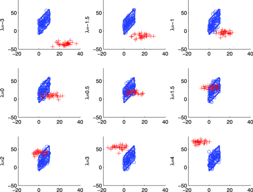
Figure 2: Example 1. Typical simulated data sets with $n_{1}=100$ and $n_{2}=30$ for nine values of $\lambda$. As $\lambda$ increases, observations from $M_{2}$ become close to those from $M_{1}$ and then become remote again. The parallelogram defines the region for the empirical overlapping index.

In Section 5 the contamination $M_{2}$ in our examples comes from a multivariate normal distribution. In the Appendix we show how to calculate the probability of intersection between this distribution and a strip around the regression plane. We call this the theoretical overlapping index. Although it ignores ${\mathcal{X}}$, it does signal cases where $y_{2}$ lies close to the regression line, even if remote from ${\mathcal{X}}$. These observations would then be “good” leverage points, in the sense that they improve the estimates of the regression parameters. For counting vertical outliers we need observations that lie in ${\mathcal{X}}$. These are signalled by the index defined in (4), which has to be calculated by simulation. We therefore call this the empirical index.

5 The Numerical Effect of Overlap: Normal Contamination

Because of the flexibility of our systematic approach, we can potentially cover a wide range of possibilities. Here we look at three numerical examples with normal contamination. In the next section we consider point contamination. We look at boxplots of the estimates over a suitable $\Lambda$ and relate these plots to the overlapping indices. We separate out the variance and bias components of the estimates and compare these through cumulative plots over $\Lambda$. Finally, we compare the estimators for their power of detecting outlying observations, that is, those that come from model 2. The detection of outliers is particularly important if we require an indication that other methods of data analysis are appropriate.

In our one-variable regression examples $M_{1}$ is the regression model $y_{i}=\alpha+\beta x_{i}+\varepsilon_{i}$, with the independent $x_{i}\sim U(a,b)$, these values generated once for all observations and values of $\lambda$. The standard deviation of $Y$ is $\sigma_{\varepsilon}$ and overlapping indices were calculated for a strip of width $\pm 2\sigma_{\varepsilon}$ around $\mathrm{E}(Y)$.

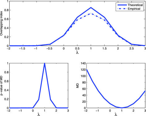
Figure 3: Example 1. Upper panel: theoretical and empirical overlapping indices for the data in Figure 2, showing maxima at $\lambda=1$. Lower panel: squared Mahalanobis distance of $M_{1}$ from $M_{2}$ (right) and corresponding $p$-values (left).

The expectation of $x$ is $\mu_{x}=(a+b)/2$. The bivariate normal distribution for $M_{2}$ has mean $\mu$ and variance $\Sigma$ given by

$$\quad\mu = \pmatrix{\alpha+\beta(\mu_{x}+d)\vspace*{2pt}\cr\mu_{x}+d}\lambda+\pmatrix{\mu_{2}\vspace*{2pt}\cr\mu_{2}}(1-\lambda)\quad\mbox{and}$$

$$\Sigma = \pmatrix{\sigma_{1}^{2}&\sigma_{12}\vspace*{2pt}\cr\sigma_{12}&\sigma_{2}^{2}},$$

where the first component corresponds to the response. When $\lambda=1$ the centres of the two populations are identical when the displacement $d=0$.

Example 1.

We took $n_{1}=100$ with $\alpha=10,\beta=3,\sigma_{\varepsilon}=10,a=0$ and $b=10$. For the second population, $n_{2}=30,\sigma_{1}^{2}=\sigma_{2}^{2}=20,\sigma_{12}=2$ and $\mu_{2}=10$. Also, $d=0$ so the centres coincide at $\lambda=1$. There were 100 simulations for each value of $\lambda$.

Figure 2 shows nine typical simulated data sets. As $\lambda$ increases from $-3$ to 4, the centre of $M_{2}$ passes through that of $M_{1}$, at which point there is almost complete overlapping of the observations from the two populations. That the overlap is not complete is shown by the plots of the indices in the upper panel of Figure 3, the maxima of which are less than one. The theoretical index is slightly higher than the empirical index, as there is some probability of observations falling within the band of $y$ values that are not in ${\mathcal{X}}$. On the other hand, the plot of the squared Mahalanobis distance from the mean of $M_{2}$ to that of $M_{1}$ has a minimum of zero, showing identity of the two centres.

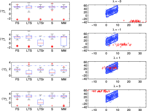
Figure 4: Example 1. Four simulated data sets for $\lambda=-3,-1,1$ and 3. Left-hand panels: boxplots, from 100 simulations, of estimates of $\beta$ (dotted and dashed line: $\beta_{1}=3$) for FS, LTS, LTSr S and MM estimators. Right-hand panels: typical simulations for these four values of $\lambda$.

We now consider the effect of these data configurations on the estimation of $\beta$. The left-hand panels of Figure 4 show boxplots, from 100 simulations, of the values of the five estimators for a series of values of $\lambda$, together with a typical data configuration for each. For $\lambda=-3$, observations from $M_{2}$ lie below and to the right of those from $M_{1}$. If these outliers are not identified, the slope of the line is decreased. The boxplots all show some simulations where such estimates occur. LTS has the highest variance amongst the estimators in the main part of the boxplot, that is, for the estimates when all outlying observations are rejected, with S the second most variable. For $\lambda=-1$, LTSr and MM are most affected by the outliers. The value $\lambda=1$ corresponds to virtually complete overlap of the two groups. All methods, on average, give estimates that are biased downwards. However, those for LTS and S are both more variable and more biased. In the last panel, for $\lambda=3$, the outliers are not as well separated as they are in panel 1. LTSr now has appreciable negative bias, due to the inclusion of outliers in the reweighting stage.

Figure 5 provides a powerful summary of the results on the variance and bias of the estimates of $\alpha$ and $\beta$ as $\lambda$ varies. The left-hand panels show the partial sums of the squared bias over $\Lambda$ and the right-hand panels show the partial sums of the variances. The values for $\alpha$ are in the top row and those for $\beta$ in the bottom row.

The plots illustrate the trade-off between bias and variance for some of the estimators. For values of $\lambda$ up to three or so, LTS and S have the highest variances and the lowest biases and have very similar properties. Over the same range LTSr and MM have high biases and low variances. The effect of the modification of LTS to LTSr and S to MM has, in general, been to reduce variance at the cost of an increase in bias. The bias values for FS are in between those of these two groups, but closer to the lower pair of values, especially for estimation of $\beta$. The variance of FS is close, and ultimately less than, the low values for LTSr and MM.

The bottom right panel of Figure 4 shows that for $\lambda=3$, the outliers are becoming distinct from $y_{1}$. As $\lambda$ increases further, the two groups become increasingly distinct, an effect that is evident in Figure 5. For the extreme values of $\lambda$, the horizontal value of the summed squared bias for all estimators shows that the bias is zero. The two populations are sufficiently far apart that the asymptotics defining high breakdown apply. This is achieved for slightly less separation by MM than LTSr. The plots of partial sums of variances, on the other hand, increase steadily, since the estimators are always subject to the effect of the random variability in the observations. The sums of variances for S and, particularly, LTS are, however, increasing more rapidly at the ends of the region than those for the other three methods, a result in line with the rows of boxplots for $\lambda=\pm 3$ in Figure 4.

These plots illustrate the differing performance of the five estimators. Since this is a paper about robust statistics, we also looked at plots in which the variance of the estimators was replaced by the average median absolute deviation from the median. These plots were close to those of the variances shown here.

In addition to good parameter estimates, we would also like our estimate to signal the presence of outliers if the model fitted to the data is incorrect. Accordingly, we calculated the average power, that is, the average number of observations correctly detected as being contaminated, which is the average number of detected observations from $M_{2}$. In testing for the presence of outliers, we used a test of Bonferronised size $\alpha^{*}$. The results are in Figure 6. Outliers are not detected for central values of $\lambda$, as the parameter estimates are sufficiently corrupted by observations from $M_{2}$ that no observations appear outlying. As the means of the two populations move apart, the number of outliers detected increases. Over most of the range FS has the highest power and LTSr the lowest. The other three estimates lie between these extremes, with MM having lower power for values of $\lambda$ near zero. As with any power curves calculated for tests whose exact sizes are not known, we need to calibrate these findings against the size of the tests (see Section 7).

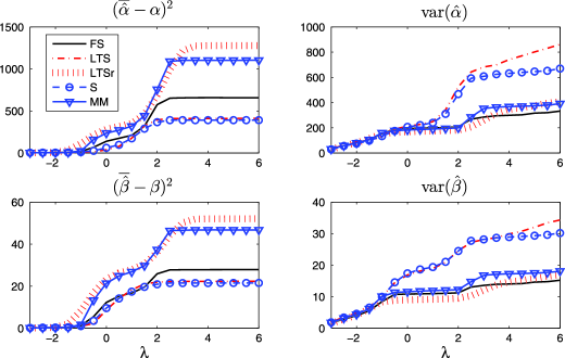
Figure 5: Example 1. Partial sums over $\Lambda$ of simulated squared bias and variance of the five estimators. Left-hand panels squared bias, right-hand panels variance. Top line $\hat{\alpha}$, bottom line $\hat{\beta}$.

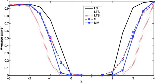
Figure 6: Example 1. Simulated average power of the five procedures over $\Lambda$.

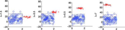
Figure 7: Example 2. Simulated data sets with $n_{1}=100$ and $n_{2}=20$ for four values of $\lambda$. As $\lambda$ increases, observations from $M_{2}$ become close to those from $M_{1}$ and then become remote again. The parallelogram defines the region for the empirical overlapping index.

Example 2.

In the interests of space we present only a part of our results, leaving the remainder for the online supplement.

We stay with a single explanatory variable but now choose a trajectory for $\lambda$ such that $\theta_{2}^{0}\neq\theta_{1}$, so that most of the observations $y_{2}$ are outlying. The parameter values for population 1 were $a=0$, $b=2$, $\alpha=10$, $\beta=1$ and $\sigma_{\varepsilon}=10$. For population 2, $\Sigma=\operatorname{diag}(4,0.1),\mu_{2}=3.4$ and $d=2$, so that the centres no longer coincided. Also, $n_{2}=20$. Figure 7 shows scatterplots of typical samples for four values of $\lambda$. In the first, for $\lambda=1.5$, there is a set of horizontal outliers, which can be expected not appreciably to affect the estimate of slope. As $\lambda$ increases, the observations from $M_{2}$ rise above those from $M_{1}$, generating increasingly remote vertical outliers.

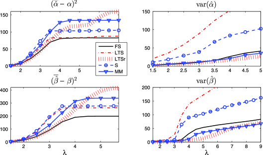
Figure 8: Example 2. Partial sums over $\Lambda$ of simulated squared bias and variance of the five estimators. Left-hand panels squared bias, right-hand panels variance. Top line $\hat{\alpha}$, bottom line $\hat{\beta}$.

The behaviour of the five estimators for this new situation is summarised in the partial sum plots of Figure 8. The plots of variances are simply interpreted: S and LTS have high variance for both $\alpha$ and $\beta$ over the whole range of $\lambda$, with MM and LTSr having low values which are slightly less than that of FS.

The comparison of biases is less straightforward. The scatterplots of Figure 7 suggest that the two populations should be adequately separated by the time $\lambda=4$. For lower values of $\lambda$, S and LTS have similar higher biases for $\beta$. The biases for $\alpha$ do not show much difference for lower values of $\lambda$. In the right-hand halves of the plots in Figure 8, with $\lambda>4$, the two populations are more separated. The plots of bias show that S and LTS provide unbiased estimates (horizontal plots) for smaller values of $\lambda$ than does MM. The LTSr estimates are not unbiased, even for the largest values of $\lambda$. The FS has excellent properties; it has the lowest bias for both parameters and a variance which is close to those from MM and LTSr.

The plot of average power for this example in Figure 19 of Riani, Atkinson and Perrotta (2014) leads to similar conclusions to those for Example 1 in Figure 6. FS has the highest power and LTSr the lowest, but now the difference between FS and the other rules is much greater. S and MM have indistinguishable performances, with LTS closer to that of LTSr.

Example 3.

The third example had five explanatory variables ($p=6$), independently uniformly distributed on ($0,2\sqrt{1}0$) with regression parameters $\beta=5$ for all variables, $\sigma_{\varepsilon}=10$ and $n_{1}=200$. For population 2, $\Sigma=\operatorname{diag}(100,I_{5}),\mu_{2}=3,d=2$ and $n_{2}=60$.

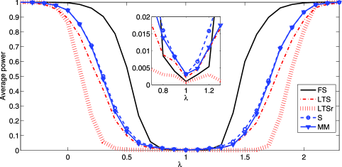
Figure 9: Example 3. Simulated average power of the five procedures over $\Lambda$ with an inset zoom of the central part of the figure.

This is a larger example, with $n_{1}=200$ and $n_{2}=60$. As $\lambda$ increases from $-1$ to 2.6, the outliers “rise through” the central observations. Since $d\neq 0$, the centres of the two distributions are never identical. Unlike our other two examples, this one does not include outliers at leverage points, so that the differences in behaviour of the methods are, to some extent, reduced.

With five explanatory variables the major contribution to the mean squared error of the parameter estimates comes from $\beta$, so we only consider these values, which are plotted in Figure 21 of Riani, Atkinson and Perrotta (2014). With independent $x_{j}$, the bias and variance are the sums of those for the individual components. LTS behaves surprisingly poorly, with the uniformly highest bias and variance. LTSr and S have medium behaviour for both properties, with the order reversed for bias and variance, while MM and FS have the same, lowest values for bias and similar values for variance until $\lambda=1$ when that for FS increases, although staying below that for S. Unlike the other two examples, the relative behaviour of the estimators is little affected by the value of $\lambda$, a reflection of the stability of the outlier pattern over $\Lambda$. Of course, the magnitude of the outliers is largest for extreme values, but leverage points are not introduced or removed.

The plot of average power is in Figure 9. As in the other plots of average power, FS has the highest power and LTSr the least. The other three estimators have very similar properties to each other. However, in assessing power we need to be sure that we are comparing tests with similar sizes. The zoom in the centre of the plot for values of $\lambda$ close to one shows that we are not, with FS and LTSr, having the smallest values. For accurate comparisons we need to scale the other three tests downwards, which will reduce the curves below the plotted values. However, even when $\lambda=1$, outliers are still present and, since $d\neq 0$, we are not looking at the null distribution of the test statistics. We consider null distributions and the resulting size of tests in Section 7.

6 The Numerical Effect of Overlap: Point Contamination

Point contamination plays an important role in the theory of robust estimation, for example, in finding conditions of maximum bias in regression (Martin, Yohai and Zamar (1989); Berrendero and Zamar (2001)). Accordingly, we extend our simulations to such contamination. Although it is a special case of (5) as $\Sigma\rightarrow 0$, there are new features.

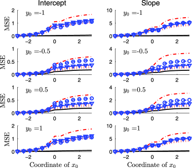
Figure 10: Point contamination at $(x_{0},y_{0})$. Partial sums of mean squared errors of estimates of $\alpha$ and $\beta$ for five values of $y_{0}$ as $x_{0}$ varies from $-3$ to 3.

The first feature is the response of the FS algorithm to several identical observations. As the search progresses, observations are not only added to the subset used in estimation, but remote observations are deleted. If several of the identical observations are included, those outside the point contamination will seem remote and the search will collapse, since the fitted model will be singular. If such singularity occurs, we identify all identical observations and force them to enter at the end of the search. As the figures show, in some cases this has a powerful beneficial effect on the estimates. The second feature is that the overlapping index now has the value of either zero or one.

We took 100 $x$ values between 0 and 1, with the normally distributed values of $y$ such that approximately 95% lay between $-0.5$ and 0.5. We add 30 identical contaminating observations at $(x_{0},y_{0})$ where both the vertical and horizontal directions of contamination range from $-3$ to 3.

Figure 10 shows plots of the partial sums of the mean squared error of the estimates of the intercept and slope for four values of $y_{0}$ over a fine grid of values of $x_{0}$ from $-3$ to 3. The most notable features are the poor performance of LTS and the good performance of FS. This is particularly striking in the more extreme vertical contaminations, $y_{0}=\pm 1$, where the FS estimates are virtually unaffected by the thirty outliers.

In Figure 11 we look at the same quantities, as $y_{0}$ varies for four fixed values of $x_{0}$: $-1$, $-0.5$, 0.5 and 1. Recall that the values of $x$ range from 0 to 1, so these plots are not symmetrical around $x_{0}=0$. The most striking feature is the excellent performance of the FS, which is by far the best except when the contamination passes through the centre of ${\mathcal{X}}$; even then it is slightly better than MM and S. LTS behaves particularly poorly when $x_{0}\in{\mathcal{X}}$, but is uniformly poorest. S and MM are similar, and slightly better than LTSr.

The use of point contamination allows sharp comparison of the algorithms for very robust regression. In the more diffuse situations of Section 5 the plots of the power curves, such as those of Figure 9, help to strengthen the comparisons.

With this two-dimensional model for contamination it is possible to explore the properties of the estimators over a grid of values for $(x_{0},y_{0})$. With higher dimensional problems, such as Example 3, we will again need to construct a trajectory $\Lambda$ along which the point contamination moves.

7 Size Comparisons

In order to establish the size of the outlier tests, we ran simulations for sample sizes $n$ from 100 to 1000 for several different dimensions of problems. The results for $p=6$ and 11 are in Figure 12. In the simulations the samples were allowed to grow with $n$, so that samples for larger values of $n$ contained those for smaller, leading to smoother curves. Both the response and the explanatory variables were simulated from independent standard normal distributions, with all regression coefficients set to one. Since all methods are affine equivariant, these arbitrary choices do not affect the results. For each value of $n$ we present the average of 10,000 simulations, in which we counted the number of samples declared as containing at least one outlier, with the tests conducted at the 1% Bonferronised level.

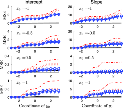
Figure 11: Point contamination at $(x_{0},y_{0})$. Partial sums of mean squared errors of estimates of $\alpha$ and $\beta$ for five values of $x_{0}$ as $y_{0}$ varies from $-3$ to 3.

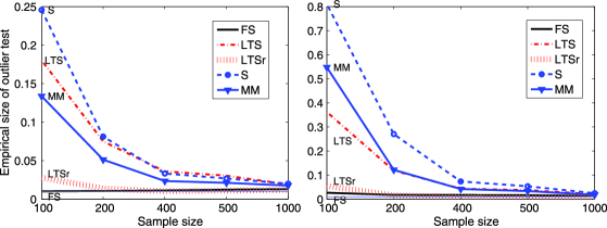
Figure 12: Size of nominally 1% Bonferronised outlier tests for, left-hand panel, $p=6$ and for $p=11$. Note the different vertical scales in the two panels.

The figure shows that, for three out of the five rules, the sizes are very far from the nominal value of 1%. For $n=100$ the sizes for MM, LTS and S when $p=6$ range between 0.13 and 0.25. For $p=11$ the range for these rules is 0.36 to 0.81. The sizes decrease with $n$, but are even so still around 2% for these rules when $n=1000$. The size for LTSr is closer to nominal, being around 3% and 6% for $n=100$ and decreasing rapidly with $n$. Only FS has a size around 1% for both values of $p$ and all $n$.

These calculations of size show that FS is correctly ordered as having highest power. The curves, such as those in Figure 9, for LTSr do not need appreciable adjustment for size. However, size adjustment for MM, LTS and S may well lead to procedures with less power than LTSr.

A simple method of adjusting power for size is a normal, or logistic, plot of the power curves, as in Figure 8.12 of Atkinson (1985), when the slope of the curve indicates power and the intercept size. Although such a comparison would be possible here, our purpose is not to establish the exact properties of outlier tests. Rather we are concerned with introducing a general framework for the comparison of methods for very robust regression.

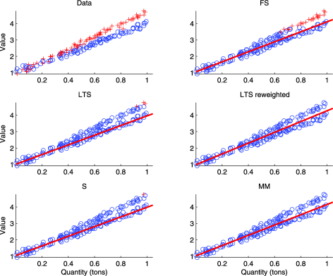
Figure 13: Trade data: results of five very robust analyses. Reading across: $\circ$ simulated regression data and outliers $+$; fitted FS line and outliers $+$; LTS, reweighted LTS, S and MM estimators.

8 Trade Data Again

We began our discussion of very robust regression in Section 2 with the trade data plotted in Figure 1. We now conclude with a plot of the fitted lines and of the outliers identified by the five methods we have been comparing. The results are in Figure 13 where the top left-hand panel repeats the plot of the data. The other panels show that FS, LTS and S all provide fits to the lower of the two lines evident for the higher values of value and quantity. The other two methods, reweighted LTS and MM, provide fitted lines which lie more between the groups. Only FS indicates that there are a large number of outliers which might perhaps be modelled separately. These results are in line with the conclusions to be expected from the simulation results of earlier sections, particularly the low power of the outlier tests for all except FS. However, the power comparisons combined with the size calculations of Section 7 show that we cannot change the level of the tests without damaging the size of the test when there no outliers and so identifying far too may outliers in the null case.

9 Discussion

The largest contrast between estimators is shown in the figures for point contamination of Section 6. The relatively poor behaviour of LTS recalls the impression of Cook and Hawkins [(1990), Section 6], that the related MVD method for multivariate data finds “Outliers Everywhere.” The superior performance of FS comes from the data-dependent flexibility of the number of observations included in the final fit.

Several authors, for example, Cook, Hawkins and Weisberg (1993) and Hawkins and Olive (2002), have commented on the persistence of the effects of the initial estimator, even asymptotically. The FS escapes such persistence because, although the subset used in fitting grows in size, observations can be deleted as well as added. This provides the algorithmic flexibility that leads to such good performance in Section 6. In addition, the flexibility of the FS combined with the plotting of diagnostic measures makes possible the detection of subpopulations in the data, not just the point contamination of Section 6. An example of cluster detection is shown in Figure 10 of Atkinson and Riani (2007).

There is also some theoretical explanation for the relative behaviour of the other estimators. In particular, the MM estimator is intended to improve the efficiency of the S estimator and, indeed, this estimator has a lower variance in Examples 1 and 2. But this is achieved at the cost of having higher bias than the S estimator. The same is true for the comparison of LTSr and LTS. For those values of ($x_{0},y_{0}$) in Section 6 for which $x_{0}\in{\mathcal{X}}$, so that there are no leverage points to introduce serious biases, LTSr and MM are, respectively, an improvement on LTS and S.

We have illustrated the use of our framework for comparing FS with methods designed to have a breakdown of 50%. Of course, the framework can be used for comparisons with breakdown levels more likely to be used in practice, such as 20% or 30%. The properties of FS, since they do not depend on a specified breakdown level, will not be changed.

Appendix: The Theoretical Overlapping Index

The response and the explanatory variables lie in a space of dimension $p+1$. Let these variables be $w$. Then the regression plane can be written as $b^{T}w-c=0$. The equation of the normal to the plane through a point $w_{0}$ on the plane is

$$z_{1}=w_{0}+bd,$$ (1)

where the scalar $d$ is the distance from the plane. The outlying observations, including the response, have a multivariate normal distribution. Let these be $W\sim{\mathcal{N}}(\mu,\Sigma)$. We require the probability that $W$ lies on one side of the plane. To obtain this, rotate $W$ to a set of variables $Z$ with $z_{1}$ (1) the normal to the plane. Integrating out the other $p$ variables shows that the required probability comes from the marginal distribution of $Z_{1}\sim{\mathcal{N}}(b^{T}\mu,b^{T}\Sigma b)$. Let the distance in the $z_{1}$ direction from $\mu$ to the plane be $d(c)$. Then, from (1), at the plane $b^{T}w=c=b^{T}\mu+b^{T}bd(c)$, so that

$$d(c)=\bigl{(}c-b^{T}\mu\bigr{)}/b^{T}b.$$ (2)

Since the distance $d(c)$ in the $z_{1}$ direction has been rescaled by the factor $1/b^{T}b$, the required probability is

$$\operatorname{Pr}\bigl{(}b^{T}W>c\bigr{)}$$

$$\quad=\operatorname{Pr}\bigl{(}Z_{1}>c-b^{T}\mu\bigr{)}$$ (3)

$$\quad=\Phi\bigl{\{}d(c)b^{T}b/\bigl{(}b^{T}\Sigma b\bigr{)}^{0.5}\bigr{\}}=\Psi(c)\quad\mbox{say},$$

where $\Phi$ is the c.d.f. of the (univariate) standard normal distribution. We require this probability in terms of the regression model, which we now write as $y=\alpha+\beta^{T}x$. Then

$$b^{T}=\bigl{(}1-\beta^{T}\bigr{)},\quad w^{T}=\bigl{(}yx^{T}\bigr{)}\quad\mbox{and}\quad c=\alpha.$$

Finally, we require the probability that $W$ lies between two planes. For any $x$ the required strip around this model is $y\pm 2\sigma_{\varepsilon}$. The two planes then are defined by constants $c^{+}=\alpha+2\sigma_{\varepsilon}$ and $c^{-}=\alpha-2\sigma_{\varepsilon}$. From (Appendix: The Theoretical Overlapping Index) the required probability is $\Psi(c^{+})-\Psi(c^{-})$.

References

- Andrews et al. (1972) {bbook}[mr] \bauthor\bsnmAndrews, \bfnmD. F.\binitsD. F., \bauthor\bsnmBickel, \bfnmP. J.\binitsP. J., \bauthor\bsnmHampel, \bfnmF. R.\binitsF. R., \bauthor\bsnmHuber, \bfnmP. J.\binitsP. J., \bauthor\bsnmRogers, \bfnmW. H.\binitsW. H. and \bauthor\bsnmTukey, \bfnmJ. W.\binitsJ. W. (\byear1972). \btitleRobust Estimates of Location: Survey and Advances. \bpublisherPrinceton Univ. Press, \blocationPrinceton, NJ. \bidmr=0331595 \bptokimsref \endbibitem
- Atkinson (1985) {bbook}[auto:STB—2013/06/05—13:45:01] \bauthor\bsnmAtkinson, \bfnmA. C.\binitsA. C. (\byear1985). \btitlePlots, Transformations, and Regression. \bpublisherOxford Univ. Press, \blocationOxford. \bptokimsref \endbibitem
- Atkinson and Riani (2000) {bbook}[mr] \bauthor\bsnmAtkinson, \bfnmAnthony\binitsA. and \bauthor\bsnmRiani, \bfnmMarco\binitsM. (\byear2000). \btitleRobust Diagnostic Regression Analysis. \bpublisherSpringer, \blocationNew York. \biddoi=10.1007/978-1-4612-1160-0, mr=1884997 \bptokimsref \endbibitem
- Atkinson and Riani (2006) {barticle}[mr] \bauthor\bsnmAtkinson, \bfnmAnthony C.\binitsA. C. and \bauthor\bsnmRiani, \bfnmMarco\binitsM. (\byear2006). \btitleDistribution theory and simulations for tests of outliers in regression. \bjournalJ. Comput. Graph. Statist. \bvolume15 \bpages460–476. \biddoi=10.1198/106186006X113593, issn=1061-8600, mr=2256154 \bptokimsref \endbibitem
- Atkinson and Riani (2007) {barticle}[mr] \bauthor\bsnmAtkinson, \bfnmA. C.\binitsA. C. and \bauthor\bsnmRiani, \bfnmM.\binitsM. (\byear2007). \btitleExploratory tools for clustering multivariate data. \bjournalComput. Statist. Data Anal. \bvolume52 \bpages272–285. \biddoi=10.1016/j.csda.2006.12.034, issn=0167-9473, mr=2409981 \bptokimsref \endbibitem
- Atkinson, Riani and Cerioli (2010) {barticle}[mr] \bauthor\bsnmAtkinson, \bfnmAnthony C.\binitsA. C., \bauthor\bsnmRiani, \bfnmMarco\binitsM. and \bauthor\bsnmCerioli, \bfnmAndrea\binitsA. (\byear2010). \btitleThe forward search: Theory and data analysis (with discussion). \bjournalJ. Korean Statist. Soc. \bvolume39 \bpages117–134. \biddoi=10.1016/j.jkss.2010.02.007, issn=1226-3192, mr=2758131 \bptnotecheck related\bptokimsref \endbibitem
- Berrendero, Mendes and Tyler (2007) {barticle}[mr] \bauthor\bsnmBerrendero, \bfnmJosé R.\binitsJ. R., \bauthor\bsnmMendes, \bfnmBeatriz V. M.\binitsB. V. M. and \bauthor\bsnmTyler, \bfnmDavid E.\binitsD. E. (\byear2007). \btitleOn the maximal bias functions of -estimates and constrained -estimates of regression. \bjournalAnn. Statist. \bvolume35 \bpages13–40. \biddoi=10.1214/009053606000000975, issn=0090-5364, mr=2332267 \bptokimsref \endbibitem
- Berrendero and Zamar (2001) {barticle}[mr] \bauthor\bsnmBerrendero, \bfnmJosé R.\binitsJ. R. and \bauthor\bsnmZamar, \bfnmRuben H.\binitsR. H. (\byear2001). \btitleMaximum bias curves for robust regression with non-elliptical regressors. \bjournalAnn. Statist. \bvolume29 \bpages224–251. \biddoi=10.1214/aos/996986507, issn=0090-5364, mr=1833964 \bptokimsref \endbibitem
- Cook and Hawkins (1990) {barticle}[auto:STB—2013/06/05—13:45:01] \bauthor\bsnmCook, \bfnmR. D.\binitsR. D. and \bauthor\bsnmHawkins, \bfnmD. M.\binitsD. M. (\byear1990). \btitleComment on Rousseeuw and van Zomeren (1990). \bjournalJ. Amer. Statist. Assoc. \bvolume85 \bpages640–644. \bptokimsref \endbibitem
- Cook, Hawkins and Weisberg (1993) {barticle}[mr] \bauthor\bsnmCook, \bfnmR. D.\binitsR. D., \bauthor\bsnmHawkins, \bfnmD. M.\binitsD. M. and \bauthor\bsnmWeisberg, \bfnmS.\binitsS. (\byear1993). \btitleExact iterative computation of the robust multivariate minimum volume ellipsoid estimator. \bjournalStatist. Probab. Lett. \bvolume16 \bpages213–218. \biddoi=10.1016/0167-7152(93)90145-9, issn=0167-7152, mr=1208510 \bptokimsref \endbibitem
- Croux and Rousseeuw (1992) {barticle}[mr] \bauthor\bsnmCroux, \bfnmChristophe\binitsC. and \bauthor\bsnmRousseeuw, \bfnmPeter J.\binitsP. J. (\byear1992). \btitleA class of high-breakdown scale estimators based on subranges. \bjournalComm. Statist. Theory Methods \bvolume21 \bpages1935–1951. \biddoi=10.1080/03610929208830889, issn=0361-0926, mr=1173503 \bptokimsref \endbibitem
- García-Escudero et al. (2010) {barticle}[mr] \bauthor\bsnmGarcía-Escudero, \bfnmL. A.\binitsL. A., \bauthor\bsnmGordaliza, \bfnmA.\binitsA., \bauthor\bsnmMayo-Iscar, \bfnmA.\binitsA. and \bauthor\bsnmSan Martín, \bfnmR.\binitsR. (\byear2010). \btitleRobust clusterwise linear regression through trimming. \bjournalComput. Statist. Data Anal. \bvolume54 \bpages3057–3069. \biddoi=10.1016/j.csda.2009.07.002, issn=0167-9473, mr=2727734 \bptokimsref \endbibitem
- Hampel (1975) {barticle}[mr] \bauthor\bsnmHampel, \bfnmFrank R.\binitsF. R. (\byear1975). \btitleBeyond location parameters: Robust concepts and methods. \bjournalBulletin of the International Statistical Institute \bvolume46 \bpages375–382. \bidmr=0483172 \bptnotecheck related\bptokimsref \endbibitem
- Hampel et al. (1986) {bbook}[mr] \bauthor\bsnmHampel, \bfnmFrank R.\binitsF. R., \bauthor\bsnmRonchetti, \bfnmElvezio M.\binitsE. M., \bauthor\bsnmRousseeuw, \bfnmPeter J.\binitsP. J. and \bauthor\bsnmStahel, \bfnmWerner A.\binitsW. A. (\byear1986). \btitleRobust Statistics: The Approach Based on Influence Functions. \bpublisherWiley, \blocationNew York. \bidmr=0829458 \bptokimsref \endbibitem
- Hawkins, Bradu and Kass (1984) {barticle}[mr] \bauthor\bsnmHawkins, \bfnmDouglas M.\binitsD. M., \bauthor\bsnmBradu, \bfnmDan\binitsD. and \bauthor\bsnmKass, \bfnmGordon V.\binitsG. V. (\byear1984). \btitleLocation of several outliers in multiple-regression data using elemental sets. \bjournalTechnometrics \bvolume26 \bpages197–208. \biddoi=10.2307/1267545, issn=0040-1706, mr=0770368 \bptokimsref \endbibitem
- Hawkins and Olive (2002) {barticle}[mr] \bauthor\bsnmHawkins, \bfnmDouglas M.\binitsD. M. and \bauthor\bsnmOlive, \bfnmDavid J.\binitsD. J. (\byear2002). \btitleInconsistency of resampling algorithms for high-breakdown regression estimators and a new algorithm (with discussion). \bjournalJ. Amer. Statist. Assoc. \bvolume97 \bpages136–159. \biddoi=10.1198/016214502753479293, issn=0162-1459, mr=1947276 \bptnotecheck related\bptokimsref \endbibitem
- Huber and Ronchetti (2009) {bbook}[mr] \bauthor\bsnmHuber, \bfnmPeter J.\binitsP. J. and \bauthor\bsnmRonchetti, \bfnmElvezio M.\binitsE. M. (\byear2009). \btitleRobust Statistics, \bedition2nd ed. \bpublisherWiley, \blocationHoboken, NJ. \biddoi=10.1002/9780470434697, mr=2488795 \bptnotecheck related\bptokimsref \endbibitem
- Maronna, Martin and Yohai (2006) {bbook}[mr] \bauthor\bsnmMaronna, \bfnmRicardo A.\binitsR. A., \bauthor\bsnmMartin, \bfnmR. Douglas\binitsR. D. and \bauthor\bsnmYohai, \bfnmVictor J.\binitsV. J. (\byear2006). \btitleRobust Statistics: Theory and Methods. \bpublisherWiley, \blocationChichester. \biddoi=10.1002/0470010940, mr=2238141 \bptokimsref \endbibitem
- Martin, Yohai and Zamar (1989) {barticle}[mr] \bauthor\bsnmMartin, \bfnmR. D.\binitsR. D., \bauthor\bsnmYohai, \bfnmV. J.\binitsV. J. and \bauthor\bsnmZamar, \bfnmR. H.\binitsR. H. (\byear1989). \btitleMin–max bias robust regression. \bjournalAnn. Statist. \bvolume17 \bpages1608–1630. \biddoi=10.1214/aos/1176347384, issn=0090-5364, mr=1026302 \bptokimsref \endbibitem
- Morgenthaler (2007) {barticle}[mr] \bauthor\bsnmMorgenthaler, \bfnmStephan\binitsS. (\byear2007). \btitleA survey of robust statistics. \bjournalStat. Methods Appl. \bvolume15 \bpages271–293. \bnoteErratum: 16 171–172. \biddoi=10.1007/s10260-007-0057-5, issn=1618-2510, mr=2394804 \bptokimsref \endbibitem
- Perrotta, Riani and Torti (2009) {barticle}[mr] \bauthor\bsnmPerrotta, \bfnmDomenico\binitsD., \bauthor\bsnmRiani, \bfnmMarco\binitsM. and \bauthor\bsnmTorti, \bfnmFrancesca\binitsF. (\byear2009). \btitleNew robust dynamic plots for regression mixture detection. \bjournalAdv. Data Anal. Classif. \bvolume3 \bpages263–279. \biddoi=10.1007/s11634-009-0050-y, issn=1862-5347, mr=2570505 \bptokimsref \endbibitem
- Pison, Van Aelst and Willems (2002) {barticle}[mr] \bauthor\bsnmPison, \bfnmG.\binitsG., \bauthor\bsnmVan Aelst, \bfnmS.\binitsS. and \bauthor\bsnmWillems, \bfnmG.\binitsG. (\byear2002). \btitleSmall sample corrections for LTS and MCD. \bjournalMetrika \bvolume55 \bpages111–123 (electronic). \biddoi=10.1007/s001840200191, issn=0026-1335, mr=1903287 \bptokimsref \endbibitem
- Riani, Atkinson and Cerioli (2009) {barticle}[mr] \bauthor\bsnmRiani, \bfnmMarco\binitsM., \bauthor\bsnmAtkinson, \bfnmAnthony C.\binitsA. C. and \bauthor\bsnmCerioli, \bfnmAndrea\binitsA. (\byear2009). \btitleFinding an unknown number of multivariate outliers. \bjournalJ. R. Stat. Soc. Ser. B Stat. Methodol. \bvolume71 \bpages447–466. \biddoi=10.1111/j.1467-9868.2008.00692.x, issn=1369-7412, mr=2649609 \bptokimsref \endbibitem
- Riani, Atkinson and Perrotta (2014) {bmisc}[auto:STB—2013/06/05—13:45:01] \bauthor\bsnmRiani, \bfnmM.\binitsM., \bauthor\bsnmAtkinson, \bfnmA. C.\binitsA. C. and \bauthor\bsnmPerrotta, \bfnmD.\binitsD. (\byear2014). \bhowpublishedSupplement to “A parametric framework for the comparison of methods of very robust regression.” DOI:\doiurl10.1214/13-STS437SUPP. \bptokimsref \endbibitem
- Riani, Perrotta and Torti (2012) {barticle}[auto:STB—2013/06/05—13:45:01] \bauthor\bsnmRiani, \bfnmM.\binitsM., \bauthor\bsnmPerrotta, \bfnmD.\binitsD. and \bauthor\bsnmTorti, \bfnmF.\binitsF. (\byear2012). \btitleFSDA: A MATLAB toolbox for robust analysis and interactive data exploration. \bjournalChemometrics and Intelligent Laboratory Systems \bvolume116 \bpages17–32. \bptokimsref \endbibitem
- Rousseeuw (1984) {barticle}[mr] \bauthor\bsnmRousseeuw, \bfnmPeter J.\binitsP. J. (\byear1984). \btitleLeast median of squares regression. \bjournalJ. Amer. Statist. Assoc. \bvolume79 \bpages871–880. \bidissn=0162-1459, mr=0770281 \bptokimsref \endbibitem
- Rousseeuw and Van Driessen (2006) {barticle}[mr] \bauthor\bsnmRousseeuw, \bfnmPeter J.\binitsP. J. and \bauthor\bparticleVan \bsnmDriessen, \bfnmKatrien\binitsK. (\byear2006). \btitleComputing LTS regression for large data sets. \bjournalData Min. Knowl. Discov. \bvolume12 \bpages29–45. \biddoi=10.1007/s10618-005-0024-4, issn=1384-5810, mr=2225526 \bptokimsref \endbibitem
- Rousseeuw and Leroy (1987) {bbook}[mr] \bauthor\bsnmRousseeuw, \bfnmPeter J.\binitsP. J. and \bauthor\bsnmLeroy, \bfnmAnnick M.\binitsA. M. (\byear1987). \btitleRobust Regression and Outlier Detection. \bpublisherWiley, \blocationNew York. \biddoi=10.1002/0471725382, mr=0914792 \bptokimsref \endbibitem
- Tallis (1963) {barticle}[mr] \bauthor\bsnmTallis, \bfnmG. M.\binitsG. M. (\byear1963). \btitleElliptical and radial truncation in normal populations. \bjournalAnn. Math. Statist. \bvolume34 \bpages940–944. \bidissn=0003-4851, mr=0152081 \bptokimsref \endbibitem
- Torti et al. (2012) {barticle}[mr] \bauthor\bsnmTorti, \bfnmFrancesca\binitsF., \bauthor\bsnmPerrotta, \bfnmDomenico\binitsD., \bauthor\bsnmAtkinson, \bfnmAnthony C.\binitsA. C. and \bauthor\bsnmRiani, \bfnmMarco\binitsM. (\byear2012). \btitleBenchmark testing of algorithms for very robust regression: FS, LMS and LTS. \bjournalComput. Statist. Data Anal. \bvolume56 \bpages2501–2512. \biddoi=10.1016/j.csda.2012.02.003, issn=0167-9473, mr=2910065 \bptokimsref \endbibitem