Unitary dynamics and finite-time measurements: a case study

Abstract

The inhibition of the decay of a quantum system by frequent measurements is known as quantum Zeno effect. Beyond the limit of projective measurements, the interplay between the unitary dynamics of the system and the coupling to a measurement apparatus becomes relevant. We explore this interplay by considering a quantum particle moving on a one-dimensional chain. A local measurement by coupling to an apparatus with a two-dimensional Hilbert space detects the presence of the particle on a specific chain site. The decay of the population is studied analytically for a two-site chain and numerically for a larger system as a function of the measurement time and the time between subsequent measurements. Particular attention is given to the shift of the energy of the measured site due to the coupling to the apparatus. The decay of the initial population can be hindered or accelerated, depending on the chosen system and the coupling parameters.

I Introduction

Quantum mechanics does not allow the observation of a system without perturbing it. This important difference to classical mechanics nowadays has lead to applications, e.g. in the detection of an eavesdropper in quantum communication gisin02 . Another spectacular effect known for almost forty years is the quantum Zeno effect misra77 ; chiu77 . Here, measurements of a system which are repeated in short time intervals can lead to a slowing-down of its dynamics which can even come to a halt when the time between subsequent measurements goes to zero.

Even though the first experiment performed on beryllium ions was initially analysed in terms of projective measurements itano90 , a more appropriate description in terms of the corresponding Bloch equations shows that the experimental results can well be understood without assuming a projective measurement block91 ; frerichs91 . In fact, while many studies of the quantum Zeno effect assume a projective measurement, a treatment of the measurement in terms of a coupling to some sort of measurement apparatus is certainly more realistic. For a recent review of a dynamical description of quantum measurements, we refer to ref. allahverdyan13 . Generalised measurements in the context of the quantum Zeno effect and their experimental realisation are discussed in mack14 .

The quantum Zeno effect with a non-projective measurement was studied for the decay of a driven two-level system coupled to an electromagnetic field ruseckas01a ; ruseckas01b . Instead of coupling the measurement device directly to the system to be measured, also indirect measurement processes have been explored where decay products are detected shaji04 ; koshino05 .

In the present paper, we are interested in the dynamics of a particle on a finite one-dimensional chain where the presence or absence of the particle at a selected site is measured by coupling to a measurement apparatus. As no decay products are generated when the particle leaves the selected site, we necessarily need to perform a direct measurement of its position.

Such a situation was first studied by Gurvitz gurvitz00 who was interested in the delocalisation induced by a local measurement on a one-dimensional disordered system described by an Anderson model. There, the transmission through a quantum point contact was used to continuously monitor the presence of an electron in one of the quantum dots of an array of coupled dots. It was found that even for very weak coupling between the electron on the quantum dot and the electrons flowing through the quantum point contact, delocalisation on the quantum dot array would ensue.

The asymptotic state, and the approach to it, of a particle moving on a chain of sites under the influence of repeated projective measurements were investigated in several works flores99 ; gordon10 ; yi11 . Here, we generalise the study presented in ref. yi11, to the case of finite-time measurements and discuss the dependence on the measurement time.

To this end, we consider the setup displayed in figure 1 where a particle can move along a one-dimensional chain containing $N+1$ sites. The presence of the particle on the left-most site of the chain indicated as site 0, is measured by an apparatus A which is coupled to this site during the measurement periods. The apparatus, its initial state and the coupling to the system to be measured is chosen according to a model proposed by Zurek zurek00 and will be described in more detail in section II.

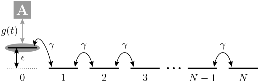
Figure 1: The setup considered here consists of a system represented by a chain of $N$ sites between which the particle can hop with an amplitude $\gamma$. The energy of the left-most site can be shifted by an amount $\epsilon$. The presence of the particle on this site is measured by coupling an apparatus A to the site with a coupling constant $g$.

According to the previous description, the Hamiltonian

$$\hat{H}=\hat{H}_{\text{c}}\otimes\openone_{\text{A}}+g(t)\hat{H}_{\text{I}}$$ (1)

consists of a part $\hat{H}_{\text{c}}$ describing the motion on the chain while $\hat{H}_{\text{I}}$ pertains to the coupling to the measurement apparatus. The unperturbed apparatus is supposed to be static with a vanishing apparatus Hamiltonian $H_{\text{A}}$. The time dependence of the coupling constant $g(t)$ ensures that the coupling is present only during measurement periods while it vanishes between them when the particle moves unobserved on the chain. The identity operator in the Hilbert space of the apparatus is denoted by $\openone_{\text{A}}$. The chain Hamiltonian is given by

$$\hat{H}_{\text{c}}=\epsilon|0\rangle\langle 0|-\gamma\sum_{n=0}^{N-1}\left(|n\rangle\langle n+1|+|n+1\rangle\langle n|\right)\,.$$ (2)

Here, the hopping matrix element is denoted by $\gamma$. The left-most site is shifted in energy relative to the other sites by an amount $\epsilon$. The explicit form of the Hamiltonian $\hat{H}_{\text{I}}$ will be given below in (10).

The measurement apparatus and the particle on the chain are supposed to be initially in a factorised state. During the measurement process, correlations are built up resulting in an entangled state. After decoupling the apparatus, the system is thus typically left in a mixed state. We will not read out the state of the apparatus and thus only carry out a premeasurement which still allows for all possible measurement outcomes. The apparatus will be reset to its initial state before it is coupled again to the left-most site.

We start by reviewing Zurek’s model in section II and adapting it to our purpose. In section III we construct a minimal model where the length of the chain consists of just two lattice sites. This minimal model allows us to study the interplay between the measurement dynamics and the system dynamics during the finite measurement time. We pay particular attention to an energy shift of the measured site due to the coupling to the measurement apparatus. Section IV is devoted to the discussion of numerical results for a chain of more than two sites and the difference of the dynamics to the case of projective measurements. Finally, in section V we present our conclusions.

II Model for the measurement apparatus

In this section we restrict ourselves to the measurement aspect of the setup displayed in figure 1 and neglect any proper dynamics of the system during the time in which the measurement apparatus is interacting with the system. We thus disregard the chain Hamiltonian $\hat{H}_{\text{c}}$ or at least assume that the system dynamics is much slower than the dynamics due to the coupling between the system and the measurement apparatus. The interplay between system dynamics and measurement process will be the subject of section III.

As a motivation for the model describing the measurement apparatus and its coupling to the chain to be used later on, we follow von Neumann vonNeumann55 and consider an apparatus with a pointer described by the continuous position operator $\hat{x}$. The initial position of the pointer is assumed to be at the origin, i.e. its initial state is given by $|0\rangle_{\text{A}}$. Here, $|0\rangle_{\text{A}}$ is the eigenstate of the operator of the pointer position $\hat{x}$ with eigenvalue 0, i.e. $\hat{x}|0\rangle_{\text{A}}=0$. Assuming that the system to be measured is in an eigenstate $|s\rangle$ of the observable

$$\hat{s}=\int\text{d}s^{\prime}s^{\prime}|s^{\prime}\rangle\langle s^{\prime}|,$$ (3)

the pointer after completion of the measurement process should be found at the position $x=s$, i.e. in the eigenstate $|s\rangle_{\text{A}}$ of the position operator $\hat{x}$ of the apparatus. Such a transition can be achieved by the translation operator

$$\hat{T}=\exp\left(-\frac{\text{i}}{\hbar}s\hat{p}\right)\,,$$ (4)

where the momentum operator $\hat{p}$ conjugate to $\hat{x}$ operates on the Hilbert space of the apparatus.

For a general initial state of the system, the coupling between system and apparatus can then be described by an interaction Hamiltonian $g(t)\hat{H}_{\text{I}}$ with

$$\hat{H}_{\text{I}}=\hat{s}\hat{p}\,.$$ (5)

The time-dependent coupling constant $g(t)$ ensures that the coupling is only present during the measurement process. By choosing its magnitude, we can control how strongly the apparatus is coupled to the system. During a measurement, when $g$ takes on a fixed value, the translation of the pointer described above can then be achieved by the time evolution operator

$$\hat{U}(t)=\exp\left(-\frac{\text{i}}{\hbar}g\hat{s}\hat{p}t\right)$$ (6)

if we choose the measurement time as $t_{\text{m}}=1/g$.

For an arbitrary initial state of the system described by the function $c(s^{\prime})$ and the apparatus in its initial state $|0\rangle_{\text{A}}$, the time evolution of system and apparatus starts from the state

$$|\Psi(0)\rangle=\int\text{d}s^{\prime}c(s^{\prime})|s^{\prime}\rangle|0\rangle_{\text{A}}\,.$$ (7)

At the end of the measurement process described by the time evolution operator (6) we obtain the entangled state

$$|\Psi(1/g)\rangle=\int\text{d}s^{\prime}c(s^{\prime})|s^{\prime}\rangle|s^{\prime}\rangle_{\text{A}}\,.$$ (8)

The value of the measured system observable $\hat{s}$ is now encoded in the pointer state of the apparatus.

For our purposes, it is sufficient to provide the apparatus with a finite Hilbert space. Since we only need to measure whether the first lattice site is occupied or not, we will eventually restrict the Hilbert space to two dimensions. For the moment, however, we assume the Hilbert space of the apparatus to be $N$-dimensional.

From the discussion above it turns out as useful to introduce, apart from the pointer states $|x\rangle_{\text{A}}$, eigenstates $|p\rangle_{\text{A}}$ of the momentum operator $\hat{p}$ conjugate to the pointer position operator $\hat{x}$. Accordingly, in the discrete case, we introduce states $\{|A_{j}\rangle_{\text{A}}\}$ and $\{|B_{k}\rangle_{\text{A}}\}$ which correspond to the pointer states and the complementary momentum basis, respectively. The two sets of states are related by

$$|A_{j}\rangle_{\text{A}}=\frac{1}{N^{1/2}}\sum_{k=0}^{N-1}\exp\left(-\frac{2\pi\text{i}}{N}jk\right)|B_{k}\rangle_{\text{A}}$$ (9)

Following ref. zurek00 , we define a discrete version of the interaction Hamiltonian between system and apparatus

$$\hat{H}_{\text{I}}=\hat{s}\hat{B}$$ (10)

with the system observable

$$\hat{s}=\sum_{k=0}^{N-1}k|s_{k}\rangle\langle s_{k}|$$ (11)

and the apparatus operator

$$\hat{B}=\sum_{k=0}^{N-1}k|B_{k}\rangle_{\text{A}}{}_{\text{A}}\langle B_{k}|\,.$$ (12)

For a measurement time

$$t_{\text{m}}=\frac{2\pi\hbar}{gN}$$ (13)

an initial state $|s_{j}\rangle|A_{0}\rangle_{\text{A}}$ evolves into

$$\exp\left(-\frac{\text{i}}{\hbar}g\hat{H}_{\text{I}}t_{\text{m}}\right)|s_{j}\rangle|A_{0}\rangle_{\text{A}}=|s_{j}\rangle|A_{j}\rangle_{\text{A}}$$ (14)

by the action of the interaction Hamiltonian (10), as required for a perfect measurement. A general initial pure state of the system will thus be turned into an entangled state between system and measurement apparatus

$$\exp\left(-\frac{\text{i}}{\hbar}g\hat{H}_{\text{I}}t_{\text{m}}\right)\sum_{j}c_{j}|s_{j}\rangle|A_{0}\rangle_{\text{A}}=\sum_{j}c_{j}|s_{j}\rangle|A_{j}\rangle_{\text{A}}\,.$$ (15)

We are now in the position to specialise the model just described to the case $N=2$. However, we also need to slightly generalise it for our purposes. As we shall see, the coupling (10) of the chain to the measurement apparatus effectively changes the on-site energy at the left-most lattice site. This effect is reminiscent of the Lamb shift due to the coupling of a bound electron to the electromagnetic field bethe47 or the potential renormalisation of a dissipative system coupled to its environment weiss12 . A change of the on-site energy on one lattice site will necessarily influence the dynamics on the chain. In addition, as an effect of the coupling to the measurement apparatus, it will be time-dependent. During the measurement process, the on-site energy will be modified while it assumes its bare value $\epsilon$ between measurements.

For the discussion of the Zeno effect on a chain, we make use of the interaction Hamiltonian (10). The system observable that detects the presence of the particle on the left-most lattice site is given by

$$\hat{s}=|0\rangle\langle 0|\,.$$ (16)

The measurement operator is obtained from (12) by setting $N=2$. In addition, for later convenience, we want to be able to shift the spectrum in order to analyse the effect of the coupling-induced shift of the energy of the measured site. We thus define

$$\hat{B}=\delta\openone_{\text{A}}-\frac{1}{2}|B_{0}\rangle_{\text{A}}{}_{\text{A}}\langle B_{0}|+\frac{1}{2}|B_{1}\rangle_{\text{A}}{}_{\text{A}}\langle B_{1}|\,,$$ (17)

where the parameter $\delta$ allows to shift the spectrum of the operator $\hat{B}$. For $\delta=1/2$, we recover the definition (12) for $N=2$.

For $N=2$, the states $\{|A_{0}\rangle_{\text{A}},|A_{1}\rangle_{\text{A}}\}$ and $\{|B_{0}\rangle_{\text{A}},|B_{1}\rangle_{\text{A}}\}$ are related by a Hadamard transform

$$\begin{pmatrix}|B_{0}\rangle_{\text{A}}\\ |B_{1}\rangle_{\text{A}}\end{pmatrix}=\frac{1}{2^{1/2}}\begin{pmatrix}1&1\\ 1&-1\end{pmatrix}\begin{pmatrix}|A_{0}\rangle_{\text{A}}\\ |A_{1}\rangle_{\text{A}}\end{pmatrix}\,.$$ (18)

Note that the Hadamard matrix equals its own inverse so that the back transformation is of the same form. Finally, the measurement time (13) becomes

$$t_{\text{m}}=\frac{\pi\hbar}{g}\,.$$ (19)

In the limit $g\to\infty$, we obtain $t_{\text{m}}=0$. It should be expected that then the limit of a projective measurement is recovered. We will check this explicitly for a two-site chain in the next section.

III Competition between system dynamics and measurement dynamics

The model discussed in this paper contains two essential ingredients. The measurement takes a finite time during which the system is coupled to the measurement apparatus. This dynamics competes with the system’s own dynamics on the finite chain.

To gain insight into the interplay between these two dynamical mechanisms, we consider a minimal model where the chain consists of two sites, one of them being measured by an apparatus with a two-dimensional Hilbert space. The corresponding Hamiltonian governing the dynamics of the combined system consisting of chain and apparatus reads

$$\hat{H} =\left[\epsilon|0\rangle\langle 0|-\gamma\big{(}|0\rangle\langle 1|+|1\rangle\langle 0|\big{)}\right]\otimes\openone_{\text{A}}$$ (20)

$$\quad+g(t)|0\rangle\langle 0|\otimes\bigg{(}\delta\openone_{\text{A}}-\frac{1}{2}|B_{0}\rangle_{\text{A}}{}_{\text{A}}\langle B_{0}|$$

$$\hskip 85.35826pt+\frac{1}{2}|B_{1}\rangle_{\text{A}}{}_{\text{A}}\langle B_{1}|\bigg{)}\,,$$

where during a measurement the coupling constant $g(t)$ takes a constant non-zero value $g$ while it vanishes during periods of free dynamics.

The bare on-site energy $\epsilon$ of the left-most site is modified by the coupling to the apparatus and becomes $\epsilon+g\delta$ during the measurement processes. We will concentrate on the special case $\epsilon=0$ and, at the end of this section, comment on how the results are modified for non-zero values of $\epsilon$.

The Hamiltonian (20) with $\epsilon=0$ can be easily diagonalised yielding the eigenenergies

$$E_{0\pm}=\frac{g}{4}(2\delta-1)\pm\left(\gamma^{2}+\frac{g^{2}}{16}(2\delta-1)^{2}\right)^{1/2}$$ (21)

and

$$E_{1\pm}=\frac{g}{4}(2\delta+1)\pm\left(\gamma^{2}+\frac{g^{2}}{16}(2\delta+1)^{2}\right)^{1/2}.$$ (22)

With

$$\tan(\phi_{0})=-\frac{4\gamma}{g(2\delta-1)}$$ (23)

and

$$\tan(\phi_{1})=-\frac{4\gamma}{g(2\delta+1)}$$ (24)

where $0\leq\phi_{0},\phi_{1}<\pi$, the corresponding eigenstates can be expressed as

$$|0+\rangle =\cos\left(\frac{\phi_{0}}{2}\right)|0\rangle|B_{0}\rangle_{\text{A}}+\sin\left(\frac{\phi_{0}}{2}\right)|1\rangle|B_{0}\rangle_{\text{A}}$$ (25)

$$|0-\rangle =\sin\left(\frac{\phi_{0}}{2}\right)|0\rangle|B_{0}\rangle_{\text{A}}-\cos\left(\frac{\phi_{0}}{2}\right)|1\rangle|B_{0}\rangle_{\text{A}}$$

and

$$|1+\rangle =\cos\left(\frac{\phi_{1}}{2}\right)|0\rangle|B_{1}\rangle_{\text{A}}+\sin\left(\frac{\phi_{1}}{2}\right)|1\rangle|B_{1}\rangle_{\text{A}}$$ (26)

$$|1-\rangle =\sin\left(\frac{\phi_{1}}{2}\right)|0\rangle|B_{1}\rangle_{\text{A}}-\cos\left(\frac{\phi_{1}}{2}\right)|1\rangle|B_{1}\rangle_{\text{A}}\,.$$

We first check whether the limit of infinite coupling, $g\to\infty$, leads to a projective measurement as expected in the previous section. As the initial state, we choose

$$|\Psi(0)\rangle=(c_{0}|0\rangle+c_{1}|1\rangle)|A_{0}\rangle_{\text{A}}$$ (27)

with complex coefficients $c_{0}$ and $c_{1}$ obeying the normalisation condition $|c_{0}|^{2}+|c_{1}|^{2}=1$. The evolution of this state is subject to the Hamiltonian (20). The result of a premeasurement is the reduced density matrix of the chain

$$\rho^{\text{S}}(t_{\text{m}})=\text{Tr}_{\text{A}}\big{(}|\Psi(t_{\text{m}})\rangle\langle\Psi(t_{\text{m}})|\big{)}$$ (28)

at the measurement time defined in (19). Here, $\text{Tr}_{\text{A}}$ denotes the trace over the Hilbert space of the apparatus. This density matrix has to be compared with the result

$$\rho_{\text{proj}}=\begin{pmatrix}|c_{0}|^{2}&0\\ 0&|c_{1}|^{2}\end{pmatrix}$$ (29)

of a projective measurement on the chain state $c_{0}|0\rangle+c_{1}|1\rangle$.

To quantify the difference between the reduced density matrix of the chain after the premeasurement $\rho^{\text{S}}(t_{\text{m}})$ and $\rho_{\text{proj}}$, we determine the trace distance

$$T(\rho^{\text{S}}(t_{\text{m}}),\rho_{\text{proj}})=\frac{1}{2}\text{Tr}_{\text{S}}\left(|\rho^{\text{S}}(t_{\text{m}})-\rho_{\text{proj}}|\right)\,,$$ (30)

where $\text{Tr}_{\text{S}}$ denotes the trace over the system Hilbert space. In the limit of large values of the coupling between system and measurement apparatus, the trace distance becomes proportional to $1/g$ or, equivalently, proportional to the measurement time $t_{\text{m}}$, i.e.,

$$T(\rho^{\text{S}}(t_{\text{m}}),\rho_{\text{proj}})=\frac{2\gamma}{g}T_{1}+O(1/g^{2})\,.$$ (31)

For a general initial state of the form (27) one finds

$$T_{1}=\left|\frac{2\delta-\sin(\pi\delta)}{1-4\delta^{2}}(c_{0}^{2}+c_{1}^{2})-\text{i}\frac{\cos(\pi\delta)}{1-4\delta^{2}}(c_{0}^{2}-c_{1}^{2})\right|\,.$$ (32)

For $\delta=0$ and an initial state (27) with $c_{0}/c_{1}=\pm 1$, the term of order $1/g$ vanishes and the projective limit is approached as $1/g^{2}$ for large $g$.

Figure 2 displays the trace distance (30) as a function of the measurement time $t_{\text{m}}=\pi\hbar/g$ for $\delta=0$. The upper curve corresponds to an initial state where the system is localised on the left lattice site. Its linear approximation according to (31) with (32) is depicted as dashed line. The lower curve with $c_{0}=c_{1}=2^{-1/2}$ represents a special case where the linear approximation vanishes and the projective limit is approached much faster than in the general case.

Figure 2: The trace distance (30) between reduced density matrices $\rho^{\text{S}}(t_{\text{m}})$ and $\rho_{\text{proj}}$ corresponding to a measurement by coupling to an apparatus and a projective measurement, respectively, is displayed as a function of the duration $t_{\text{m}}$ of the measurement for $\delta=0$ and $\gamma=1$. The upper curve corresponds to an initial state of the form (27) with $c_{0}=1$ and $c_{1}=0$. The dashed line represents its linear approximation given by (31) with (32). The lower curve with $c_{0}=c_{1}=2^{-1/2}$ represents a special case where the linear term vanishes.

The dependence of the coefficient $T_{1}$ appearing in the linear approximation of the trace distance (30) on $\delta$ is shown in figure 3 for an initial state of the form (27) with $c_{0}=1$ and $c_{1}=0$. The maximum at $\delta=0$ can be explained in terms of the system dynamics during the measurement. A non-zero value of $\delta$ effectively shifts the on-site energy of the left site out of resonance with the right site, thus suppressing the system dynamics. As a consequence $T_{1}$ decreases with increasing absolute values of $\delta$. For degenerate on-site energies on the chain, approaching the projective limit requires a particularly short measurement time $t_{\text{m}}$ or, equivalently, strong coupling between chain and measurement apparatus.

Figure 3: The coefficient $T_{1}$ defined in (32) as a function of the parameter $\delta$ for an initial state of the form (27) with $c_{0}=1,c_{1}=0$.

The influence of the system dynamics on a finite-time measurement implies that the resulting state of system and apparatus is not given by (14) where the system dynamics was neglected completely. For the initial state

$$|\Psi(0)\rangle=|0\rangle|A_{0}\rangle_{\text{A}}$$ (33)

one finds for the state at the end of the measurement process to leading order in the inverse coupling constant

$$|\Psi(t_{\text{m}})\rangle =\text{ie}^{-\text{i}\pi\delta}|0\rangle|A_{1}\rangle_{\text{A}}$$ (34)

$$\quad+\frac{\gamma}{g}\left(\frac{1-\text{ie}^{-\text{i}\pi\delta}}{2\delta-1}+\frac{1+\text{ie}^{-\text{i}\pi\delta}}{2\delta+1}\right)|1\rangle|A_{0}\rangle_{\text{A}}$$

$$\quad+\frac{\gamma}{g}\left(\frac{1-\text{ie}^{-\text{i}\pi\delta}}{2\delta-1}-\frac{1+\text{ie}^{-\text{i}\pi\delta}}{2\delta+1}\right)|1\rangle|A_{1}\rangle_{\text{A}}$$

$$\quad+O(1/g^{2})\,.$$

The first term corresponds to a measurement that is not influenced by the system dynamics. For $\delta=1/2$, it agrees with the expected state $|0\rangle|A_{1}\rangle_{\text{A}}$, where the state $|A_{1}\rangle_{\text{A}}$ indicates the presence of the particle on the measured site 0. A contribution with the particle on site 0 and the apparatus in state $|A_{0}\rangle_{\text{A}}$ is only found if terms of order $1/g^{2}$ are retained.

The influence of the system dynamics on the state resulting from a measurement can again be quantified by means of the trace distance. To leading order in $1/g$, the trace distance between the density matrix $\rho(t_{\text{m}})=|\Psi(t_{\text{m}})\rangle\langle\Psi(t_{\text{m}})|$ and the density matrix $\rho_{0}=|0\rangle\langle 0|\otimes|A_{1}\rangle_{\text{A}}{}_{\text{A}}\langle A_{1}|$ is found as

$$T(\rho(t_{\text{m}}),\rho_{0})=\frac{2^{3/2}\gamma}{g}T_{1}^{\prime}+O(1/g^{2})$$ (35)

with

$$T_{1}^{\prime}=\left[\frac{1-\sin(\pi\delta)}{2(2\delta-1)^{2}}+\frac{1+\sin(\pi\delta)}{2(2\delta+1)^{2}}\right]^{1/2}\,.$$ (36)

The latter expression agrees with (32) for $c_{0}=1,c_{1}=0$. The dependence on the parameter $\delta$ of the perturbation of the measurement result by the system dynamics can thus again be inferred from figure 3 and the corresponding discussion given above.

After having explored how the system dynamics perturbs the measurement process, we now address the question of how the system dynamics is affected by the coupling to the measurement apparatus. To this end we consider the probability to find the particle on site 0

$$\rho_{00}^{\text{S}}(t)=\langle 0|\rho^{\text{S}}(t)|0\rangle\,,$$ (37)

where the reduced density matrix of the system has been defined in (28).

Starting from the pure initial state

$$|\Psi(0)\rangle=|0\rangle|A_{0}\rangle_{\text{A}}\,,$$ (38)

diagonalisation of the Hamiltonian (20) yields

$$\rho^{S}_{00}(t)=1+\frac{\gamma^{2}}{\hbar^{2}}\left[\frac{\cos(\Omega_{0}t)-1}{\Omega_{0}^{2}}+\frac{\cos(\Omega_{1}t)-1}{\Omega_{1}^{2}}\right]\,.$$ (39)

Here,

$$\Omega_{n}=\frac{E_{n+}-E_{n-}}{\hbar}\quad\text{for $n=0,1$}$$ (40)

are differences of the energies defined in (21) and (22). Of particular interest is the decay of the population on the left site of the chain which for short times is given by

$$\rho_{00}^{\text{S}}(t)=1-\frac{\gamma^{2}t^{2}}{\hbar^{2}}+\frac{1}{3}\left(1+\frac{g^{2}(4\delta^{2}+1)}{16\gamma^{2}}\right)\frac{\gamma^{4}t^{4}}{\hbar^{4}}+O(t^{6})\,.$$ (41)

The leading decay term of second order in $t$ is exclusively due to the hopping between the two sites of the chain. The coupling to the measurement apparatus appears first in fourth order in $t$ and tends to delay the decay of the population on the measured site. Including a non-zero value for $\delta$ in the coupling part of (20) helps to suppress further the dynamics on the chain.

In figure 4 the survival probability is presented during a measurement with coupling constant $g/\gamma=\pi$. Clearly, increasing $\delta$ tends to hinder the dynamics on the chain in agreement with the fourth-order term in (41). Compared to the free dynamics on the chain, $g/\gamma=0$, depicted as dashed line, this effect is visible for all values of $\delta$. Only at the beginning of the measurement process, the decay is independent of the coupling to the measurement apparatus as expressed by the second-order term in (41).

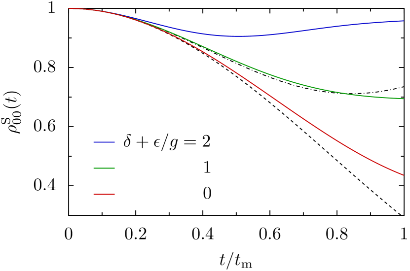
Figure 4: The survival probability on the left site of the chain during a measurement with $g/\gamma=\pi$ is shown for $\delta+\epsilon/g=0,1$, and $2$ increasing from the lower to the upper solid line. The free evolution in the absence of an apparatus, i.e. $g=0$, is depicted as dashed line for degenerate on-site energies and as dash-dotted line if the left site is lowered by $\epsilon/\gamma=-\pi$ with respect to the right site.

However, the energy shift induced by the coupling to the apparatus can also enhance the decay of the initial chain state. This is the case if the two on-site energies are not degenerate, i.e. if the energy shift $\epsilon$ in the chain part of the Hamiltonian (20) is non-zero. As we have discussed when introducing that Hamiltonian, the energy of site 0 under the influence of the coupling to the apparatus is given by $\epsilon+g\delta$. The fastest decay of the initial state is then no longer obtained for $\delta=0$ but for $\delta=-\epsilon/g$. In figure 4, the dash-dotted line depicts the time dependence of $\rho_{00}^{\text{S}}(t)$ in the absence of a coupling to the apparatus and for an energy shift of $\epsilon/\gamma=-\pi$. For $\delta=1$, corresponding to $\delta+\epsilon/g=0$ in the figure, the decay of the initial state is optimally accelerated.

IV Repeated measurements

So far, we have focussed on the interplay between the system dynamics and the coupling to the apparatus during a single measurement process. Now, we will consider repeated measurements. At the beginning of the $n$-th measurement, the particle on the chain will generally be in a mixed state described by the density matrix $\rho_{n}^{\text{S}}$. The initial state of the apparatus will always be given by the pure state $|A_{0}\rangle_{\text{A}}$ as explained in section II. During the $n$-th measurement process, an entangled state between system and apparatus will evolve which at the end of the measurement is described by a density matrix $\rho_{n}$. We will not read out the measurement result and thus account for all sequences of measurement outcomes during the repeated measurements.

After the $n$-th measurement, the free system dynamics starts with an initial density matrix $\text{Tr}_{\text{A}}(\rho_{n})$ where the degrees of freedom of the apparatus have been traced out. At the end of the free time evolution, the system state is given by the density matrix $\rho_{n+1}^{\text{S}}$. One cycle spanning the time between the beginning of subsequent measurement processes can then be described by the sequence of density matrices

$$\rho_{n}^{\text{S}}\otimes|A_{0}\rangle_{\text{A}}{}_{\text{A}}\langle A_{0}|\rightarrow\rho_{n}\rightarrow\text{Tr}_{\text{A}}(\rho_{n})\rightarrow\rho_{n+1}^{\text{S}}$$ (42)

$$\rightarrow\rho_{n+1}^{\text{S}}\otimes|A_{0}\rangle_{\text{A}}{}_{\text{A}}\langle A_{0}|$$

The relevant times involved in such a cycle are depicted in figure 5. The duration $t_{\text{m}}$ of a single measurement is related to the coupling constant $g$ between system and apparatus by (19). After the measurement, a period of length $t_{\text{f}}$ follows where the system is decoupled from the apparatus and evolves freely. The lapse of time between the beginning of subsequent measurements is then given by $t_{\text{d}}=t_{\text{m}}+t_{\text{f}}$. For the following discussion it should be kept in mind that obviously the time span $t_{\text{d}}$ can never be smaller than the duration of a measurement $t_{\text{m}}$.

Figure 5: Time scales involved in repeated measurements: Measurements of duration $t_{\text{m}}$ are separated by periods of duration $t_{\text{f}}$ of free evolution. The time between the beginning of subsequent measurements is $t_{\text{d}}=t_{\text{m}}+t_{\text{f}}$. The coupling strength between system and apparatus satisfies (19).

The results for the probability $\rho_{00}^{\text{S}}$ to find the particle on the left-most chain site presented in the figures of this section have been calculated numerically for a chain of 15 sites. For $\epsilon/\gamma=0$, the maximum group velocity on the chain is given by $2\gamma/\hbar$, so that in the absence of any measurements a particle initially located on site 0 can be expected to reappear there for the first time when $\gamma t/\hbar\sim 15$. This estimation is found to be correct even in the presence of projective measurements yi11 and can be expected to hold also for finite-time measurements. In order to avoid effects arising from reflections at the right end of the chain, we will choose times smaller than $15\hbar/\gamma$.

First, in figure 6, we compare the time dependence of $\rho_{00}^{\text{S}}$ for different energy offsets $\epsilon$ on site 0 and different durations $t_{\text{f}}$ of the free dynamics. The strength of the coupling between system and apparatus is always given by $g/\gamma=100$ corresponding to a measurement time $\gamma t_{\text{m}}/\hbar=\pi/100$ and $\delta=0$. The times at which measurements occur are indicated by arrows.

In the lower (red) solid curve, all on-site energies are degenerate and the time between measurements is $\gamma t_{\text{f}}/\hbar=0.9$. Up to the first measurement, $\rho_{00}^{\text{S}}(t)$ follows the free dynamics for $\epsilon/\gamma=0$ depicted by the lower dashed curve. Comparing the two curves one sees that the measurements tend to hinder the decay of the population on site 0.

It is interesting to compare the case of degenerate on-site energies with the case where the site 0 is shifted in energy by an amount $\epsilon/\gamma=\pi$. The corresponding free evolution of $\rho_{00}^{\text{S}}(t)$ is given by the upper dashed curve. Clearly, the energy shift makes it difficult for the particle to leave its initial site. However, frequent measurements like in the middle (black) solid curve for $\gamma t_{\text{f}}/\hbar=0.9$ assist the decay of the population on site 0. Increasing the intervals between the measurements, the population decay slows down as can be seen from the upper (blue) solid curve which has been obtained for $\gamma t_{\text{f}}/\hbar=2$.

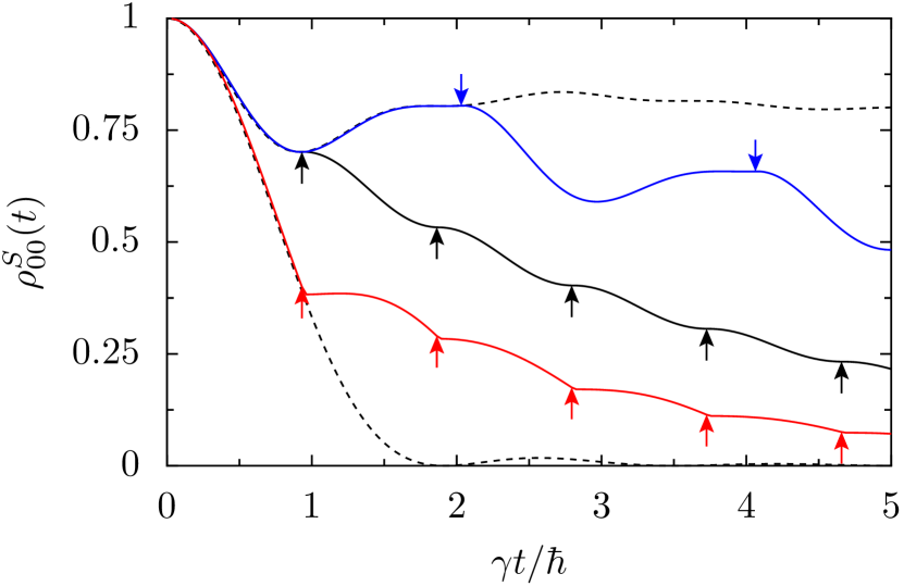
Figure 6: The time dependence of the probability to find the particle on site 0 is shown for a chain consisting of 15 sites. The lower dashed curve and the lowest (red) solid curve refer to $\epsilon/\gamma=0$ while the upper dashed curve and the two upper (black and blue) solid curves have been obtained for an energy shift of site 0 of $\epsilon/\gamma=\pi$. The solid curves show the time evolution for measurements with $\gamma t_{\text{m}}/\hbar=\pi/100$ or $g/\gamma=100$ at times indicated by the arrows. For the two lower (red and black) solid curves, the periods of free dynamics are of length $\gamma t_{\text{f}}/\hbar=0.9$ while for the upper (blue) solid curve, we have chosen $\gamma t_{\text{f}}/\hbar=2$. The dashed curves result from the free dynamics on the chain without any measurements. For all curves we have set $\delta=0$.

A more complete picture of the time evolution of the population on site 0 for fixed measurement time $\gamma t_{\text{m}}/\hbar=\pi/100$ or $g/\gamma=100$ and variable period of free dynamics of length $\gamma t_{\text{f}}/\hbar$ is given in figure 7(a) for $\epsilon/\gamma=0$ and in figure 7(b) for $\epsilon/\gamma=\pi$. In both figures, the parameter $\delta$ is set to zero but, because of the short measurement time, its value does not affect the results much. The horizontal white lines indicate the cuts represented by the solid curves in figure 6.

If all on-site energies are degenerate, the particle can easily leave its initial site 0 and move along the chain. The corresponding fast decay of $\rho_{00}^{\text{S}}$ can clearly be seen in figure 7(a) for sufficiently large values of $t_{\text{f}}$. However, as the distance between the measurements is decreased, the decay of $\rho_{00}^{\text{S}}$ is slowed down. For very small values of $t_{\text{f}}$, the particle remains on site 0 for a very long time thereby manifesting the quantum Zeno effect.

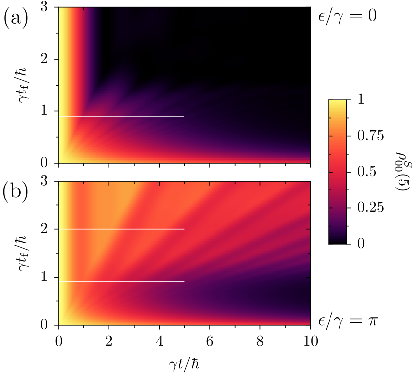
Figure 7: The occupation of site 0 is shown as function of time $t$ and the period of free evolution $t_{\text{f}}$ for finite-time measurements of a short duration $\gamma t_{\text{m}}/\hbar=\pi/100$. The chain consists of 15 sites with the energy offset (a) $\epsilon/\gamma=0$ and (b) $\epsilon/\gamma=\pi$. In the coupling Hamiltonian we have set $\delta=0$. The white lines indicate the cuts displayed as solid curves in figure 6.

The scenario just described should be contrasted with the case where the energy of site 0 is shifted with respect to the energies of the other sites of the chain. Comparing figure 7(b), where $\epsilon/\gamma=\pi$, with the previously discussed figure 7(a) we note, that they resemble each other for small values of $t_{\text{f}}$. With increasing $t_{\text{f}}$, the decay of the population on site 0 accelerates and the quantum Zeno effect becomes less effective. Increasing $t_{\text{f}}$ even further, the free dynamics becomes dominant and the nonzero value of the energy shift $\epsilon$ tends to suppress the decay of $\rho_{00}^{\text{S}}$. As a consequence, the decay is slowest for $\gamma t_{\text{f}}/\hbar\lesssim 1$, i.e. when the time between measurements is somewhat smaller than the time scale of the free dynamics.

So far, we have kept the measurement time $t_{\text{m}}$ constant. Now, we want to study the decay of $\rho_{00}^{\text{S}}$ as a function of the measurement time and the time between measurements. Since the time between measurements can be specified either in terms of $t_{\text{f}}$ or $t_{\text{d}}$ (cf. figure 5), we obtain two different representations shown in figures 8 and 9. In these figures, the decay of $\rho_{00}^{\text{S}}$, relative to its initial value $\rho_{00}^{\text{S}}(0)=1$, is represented by its value at time $\gamma t/\hbar=5$. Of course, only for special values of $t_{\text{m}}$ and $t_{\text{f}}$ will the time $\gamma t/\hbar=5$ coincide with the beginning or end of a measurement process. We consider a setup where all on-site energies are degenerate, i.e. $\epsilon/\gamma=0$. Furthermore, we choose $\delta=3/2$ which results in a strong suppression of the decay of $\rho_{00}^{\text{S}}$ during the measurement process.

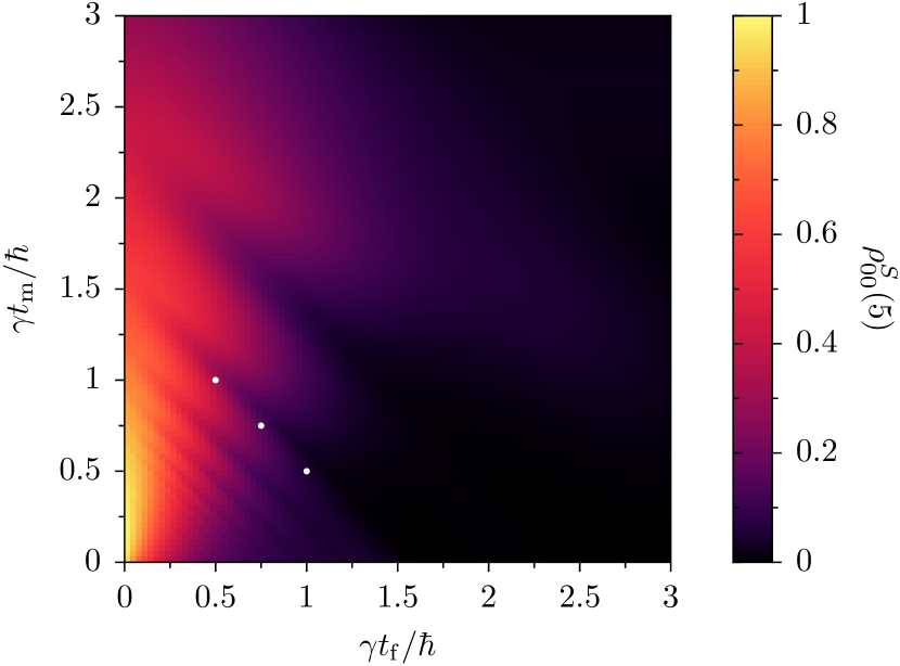
Figure 8: The occupation of site 0 at time $\gamma t/\hbar=5$ is shown as a function of the measurement duration $t_{\text{m}}$ and the period of free evolution $t_{\text{f}}$ for a chain consisting of 15 sites. All on-site energies are degenerate, $\epsilon/\gamma=0$, and $\delta=3/2$. The white points mark the parameters for which the time evolution of $\rho_{00}^{\text{S}}$ is shown in figure 10.

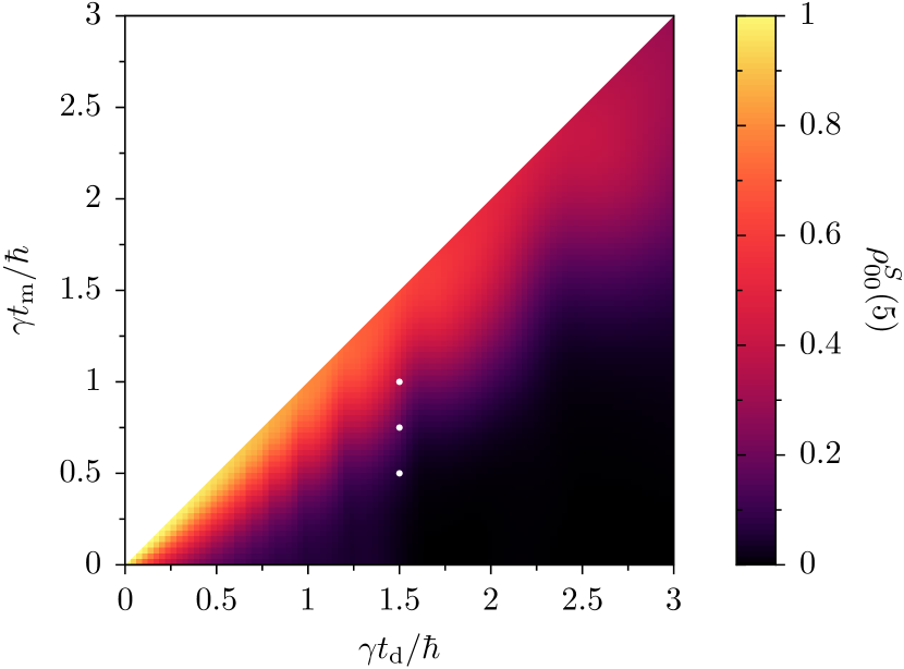
Figure 9: The data from figure 8 are now shown as a function of the measurement duration $t_{\text{m}}$ and the time $t_{\text{d}}=t_{\text{f}}+t_{\text{m}}$ between the beginning of two subsequent measurements. In the upper left white triangle, $t_{\text{f}}$ would be negative. The white points mark the parameters for which the time evolution of $\rho_{00}^{\text{S}}$ is shown in figure 10.

In figure 8, the occupation on site 0 is represented as a function of $t_{\text{m}}$ and $t_{\text{f}}$. For short times $t_{\text{f}}$ between measurements and measurement durations of up to $\gamma t_{\text{m}}/\hbar\sim 1$, one finds a strong inhibition of the decay of the occupation. This decay weakens as the period of free system evolution is increased. For long measurement durations $t_{\text{m}}$, in view of (19) the coupling between the system and the apparatus is very weak. The time dependence of the occupation on site 0 is then dominated by the system dynamics. The occupation is thus strongly suppressed at $\gamma t/\hbar=5$.

Interestingly, for sufficiently large values of $\delta$ like the one chosen for figures  8–10, there exists an intermediate regime for $t_{\text{m}}$ where $\rho_{00}^{\text{S}}$ as a function of $t_{\text{f}}$ does not decrease as fast as in the limits of small and large $t_{\text{m}}$. In this regime, the energetic degeneracy of site 0 and the other sites is lifted sufficiently strongly for a long enough time to lead to an appreciable suppression of the decay.

This effect is also visible in figure 9 where the same data are represented as in figure 8 but now as a function of $t_{\text{m}}$ and $t_{\text{d}}$. Since the time between the beginning of subsequent measurement processes has to be larger than the measurement time itself, only the lower right triangle contains data. The quantum Zeno effect is visible for small values of $t_{\text{d}}$ close to the diagonal. For not too large fixed times $t_{\text{d}}$ between the beginning of subsequent measurements, an increase of the measurement time $t_{\text{m}}$ leads to an increase of $\rho_{00}^{\text{S}}$ at a fixed time $t$. For large values of $t_{\text{d}}$, the reflection of the particle at the far end of the chain will become relevant.

Figure 10 shows how the values of $\rho_{00}^{\text{S}}(5)$ depicted in figures 8 and 9 are approached as a function of time for the parameters indicated in the latter figures by white points. The time between subsequent measurements $\gamma t_{\text{d}}/\hbar=1.5$ is kept fixed while the measurement time is different for the three curves. The time evolution during the measurement periods is indicated by thick lines. Except for short times, an increase of the measurement time will help to inhibit the decay of the population on site 0. As already indicated above, this dependence on the measurement time will only be noticeable if the energy shift induced by the coupling to the measurement apparatus is sufficiently strong, i.e. if $\delta$ is sufficiently large.

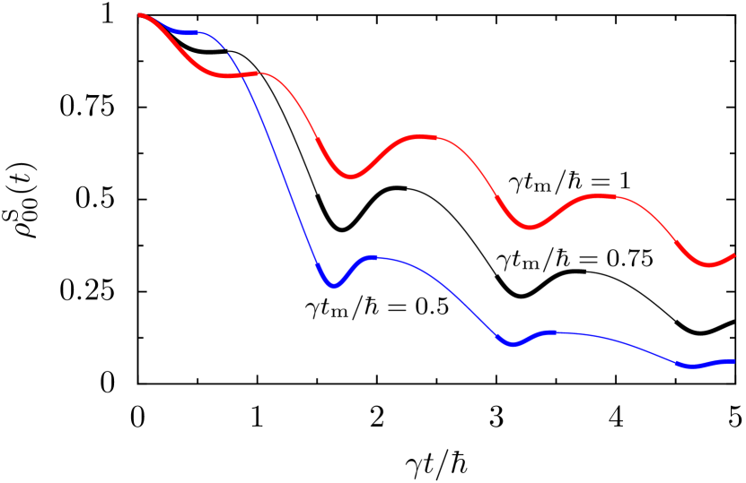
Figure 10: The occupation of site 0 of a chain consisting of 15 sites with $\epsilon/\gamma=0$ is shown as a function of time for measurement durations $\gamma t_{\text{m}}/\hbar=0.5,0.75,$ and $1$. The time evolution during the measurement processes is depicted by the thick line segments. The time between the beginning of subsequent measurements is $\gamma t_{\text{d}}/\hbar=1.5$ for all three curves and $\delta=\frac{3}{2}$.

V Conclusions

We have studied the decay of the population on a lattice site of a one-dimensional chain under the influence of a local finite-time measurement. Our setup provides a simple model to explore the interplay between the system dynamics and the coupling to the measurement apparatus. For the special case of a two-site chain, we have shown analytically, that the limit of infinite coupling to the apparatus leads to a projective measurement. For finite values of the coupling constant, we found that a shift $\delta$ of the eigenspectrum of the observable conjugate to the pointer variable modifies the on-site energy during the measurement in a significant way. Depending on the bare on-site energy and the value of $\delta$, the decay of the population on the measured site can be hindered or facilitated. If the measured site is not energetically degenerate with the other sites, numerical results for a longer chain showed that the decay is fastest for an intermediate value of the time between measurements. While for shorter periods of free dynamics, the quantum Zeno effect dominates, it is the unitary dynamics of the system which suppresses the decay if measurements occur infrequently. On the other hand, for a chain with degenerate energies, the coupling-induced shift of the on-site energy leads to a suppression of the decay for intermediate values of the measurement time. In contrast, for short measurement times, the shift is effective only during a too short time while for large measurement times, the coupling to the apparatus is weak and the shift becomes again irrelevant.

References

- (1) Gisin N, Ribordy G, Tittel W, and Zbinden H 2002 Rev. Mod. Phys. 74 145
- (2) Misra B and Sudarshan ECG 1977 J. Math. Phys. 18 756
- (3) Chiu CB, Sudarshan ECG, and Misra B 1977 Phys. Rev. D 16 520
- (4) Itano WM, Heinzen DJ, Bollinger JJ, and Wineland DJ 1990 Phys. Rev. A 41 2295
- (5) Block E and Berman PR 1991 Phys. Rev. A 44 1466
- (6) Frerichs V and Schenzle A 1991 Phys. Rev. A 44 1962
- (7) Allahverdyan AE, Balian R, Nieuwenhuizen TM 2013 Phys. Rep. 525 1
- (8) Mack G, Wallentowitz S, and Toschek PE 2014 to appear in Phys. Rep.
- (9) Ruseckas J and Kaulakys B 2001 Phys. Rev. A 63 062103
- (10) Ruseckas J 2001 Phys. Lett. A 291, 185
- (11) Shaji A 2004 J. Phys. A: Math. Gen. 37, 11285
- (12) Koshino K and Shimizu A 2005 Phys. Rep. 412, 191
- (13) Gurvitz SA 2000 Phys. Rev. Lett. 85 812
- (14) Flores JC 1999 Phys. Rev. B 60 30
- (15) Gordon G, Rao DDB, and Kurizki G 2010 New J. Phys. 12 053033
- (16) Yi J, Talkner P, and Ingold G-L 2011 Phys. Rev. A 84 032121
- (17) Zurek WH 2000 Ann. Phys. (Leipzig) 9 855
- (18) von Neumann J 1955 Mathematical foundations of quantum mechanics, Chap VI.3 (Princeton University Press, Princeton)
- (19) Bethe HA 1947 Phys. Rev. 72 339
- (20) Weiss U 2012 Quantum Dissipative Systems, edition (World Scientific, Singapore)