Redshift evolution of extragalactic rotation measures

Abstract

We obtained rotation measures of 2642 quasars by cross-identification of the most updated quasar catalog and rotation measure catalog. After discounting the foreground Galactic Faraday rotation of the Milky Way, we get the residual rotation measure (RRM) of these quasars. We carefully discarded the effects from measurement and systematical uncertainties of RRMs as well as large RRMs from outliers, and get marginal evidence for the redshift evolution of real dispersion of RRMs which steady increases to 10 rad m^-2 from $z=0$ to $z\sim 1$ and is saturated around the value at higher redshifts. The ionized clouds in the form of galaxy, galaxy clusters or cosmological filaments could produce the observed RRM evolutions with different dispersion width. However current data sets can not constrain the contributions from galaxy halos and cosmic webs. Future RM measurements for a large sample of quasars with high precision are desired to disentangle these different contributions.

1 Introduction

Faraday rotation is a powerful tool to probe the extragalactic medium. The observed rotation measure of a linearly polarized radio source at redshift $z_{\rm s}$ is determined by the polarization angle rotation ($\psi_{1}-\psi_{2}$) against the wavelength square ($\lambda_{1}^{2}-\lambda_{2}^{2}$)

$$RM_{\rm obs}=\frac{\psi_{1}-\psi_{2}}{\lambda_{1}^{2}-\lambda_{2}^{2}}=0.81\int_{z_{s}}^{0}\frac{n_{e}(z)B_{||}(z)}{(1+z)^{2}}\frac{dl}{dz}dz.$$ (1)

The rotation measure (RM, in the unit of rad m^-2) is an integrated quantity of the product of thermal electron density ($n_{\rm e}$, in the unit of cm^-3) and magnetic fields along the line of sight ($B_{||}$, in the unit of $\mu$G) over the path from the source at a redshift $z_{\rm s}$ to us. Here the comoving path increment per unit redshift, $dl/dz$, is in parsecs. The observed rotation measure, $RM_{\rm obs}$, with a uncertainty, $\sigma_{RM}$, is a sum of the rotation measure intrinsic to the source, $RM_{\rm in}$, the rotation measure in intergalactic space, $RM_{\rm IGM}$, the foreground Galactic RM, $GRM$, from our Milky Way Galaxy, i.e.

$$RM_{\rm obs}=RM_{\rm in}+RM_{\rm IGM}+GRM.$$ (2)

It has been found that the RM distribution of radio sources in the sky are correlated in angular scale of a few degree to a few tens degree (Simard-Normandin & Kronberg, 1980; Oren & Wolfe, 1995; Han et al., 1997; Stil, Taylor & Sunstrum, 2011), which indicates the smooth Galactic RM foreground. The extragalactic rotation measures is $RM_{\rm in}+RM_{\rm IGM}=RM_{\rm obs}-GRM$, which is often called as residual rotation measure (RRM), i.e. the residual after the foreground Galactic RM is discounted from the observed RM. Because the polarization angle undergoes a random walk in the intergalactic space due to intervening magnetoionic medium, the RRMs from the intergalactic medium should have a zero-mean Gaussian distribution. Radio sources at higher redshift will pass through more intervening medium, so that variance of RRMs, $V_{\rm RRM}$, of a sample of sources is expected to get larger at higher redshifts. Though the measured RM values from a source could be likely wavelength dependent due to unresolved multiple components (Farnsworth, Rudnick & Brown, 2011; Xu & Han, 2012; Bernet, Miniati & Lilly, 2012), RM values intrinsic to a radio source at redshift $z_{\rm s}$ are reduced by a factor $(1+z_{\rm s})^{−2}$ due to change of $\lambda$ when transformed to the observer’s frame, and for the variance by a factor $(1+z_{\rm s})^{−4}$, the RRMs are therefore often statistically used to probe magnetic fields in the intervening medium between the source and us, such as galaxies, galaxy clusters or cosmic webs.

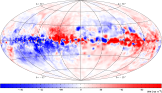
Figure 1: Sky view for the foreground Galactic RM derived by Oppermann et al. (2012) (the top panel) and by Xu & Han (2014) (the middle panel), and their difference (the bottom panel). See Xu & Han (2014) for details.

Previously there have been many efforts to investigate RRM distributions and their possible evolution with redshift. Without a good assessment of the foreground Galactic RM in early days, RMs of a small sample of radio sources gave some indications for larger RRM data scatter at higher redshifts, which were taken as evidence of magnetic field in the intergalactic medium (Nelson, 1973; Vallee, 1975; Kronberg & Simard-Normandin, 1976; Kronberg, Reinhardt & Simard-Normandin, 1977; Thomson & Nelson, 1982). Burman (1974) proposed the steady-state model and found that the variance of RRM approaches a limiting value at $z_{s}\sim 1$; Kronberg, Reinhardt & Simard-Normandin (1977) suggested $\sigma_{\rm IGM}<10$ rad m^-2; Vallee (1975) claimed the upper limit of intergalactic rotation measure as being 10 rad m^-2. Theoretical models for the random intergalactic magnetic fields in the Friedmann cosmology (Nelson, 1973) and in Einstein-de Sitter cosmology (Burman, 1974) and for the uniform fields (Vallee, 1975) have been proposed. Thomson & Nelson (1982) summarized the Friedmann model (Nelson, 1973) and the steady-state model (Burman, 1974) and also proposed their own ionized cloud model. In Friedmann model, particles conservation is assumed and the field is frozen in the evolving Friedmann cosmology, Thomson & Nelson (1982) showed $V_{\rm RRM}$ increasing with $(1+z)^{3\sim 4}$ depending on cosmology density $\Omega_{M}$. In the steady-state model contiguous random cells do not vary with time, which induces the intergalactic $V_{\rm RRM}\propto[1-(1+z_{s})^{-4}]$. In the ionized cloud model, the Faraday-active cells with random fields are in the form of non-evolving discrete gravitationally bound, ionized clouds, so that the final $V_{\rm RRM}\propto[1-(1+z_{s})^{-2}]$. Thomson & Nelson (1982) applied these three models to fit the increasing RM variance of 134 quasars against redshift, but can not distinguish the models due to large uncertainties. Welter, Perry & Kronberg (1984) made a statistics of the RRMs of 112 quasars and found a systematic increase of $V_{\rm RRM}$ with redshift even up to redshift $z$ above 2. After considering possible contributions to the RRM variance from RMs intrinsic to quasars or from RMs due to discrete intervening clouds, Welter, Perry & Kronberg (1984) suggest that the observed RRM variance mainly results from absorption-line associated intervening clouds.

Because intervening galaxies are most probable clouds for the intergalactic RMs at cosmological distances, efforts to search for evidence for the association between the enlarged RRM variance with optical absorption-lines of quasars therefore have been made for many years, first by Kronberg & Perry (1982), later by Welter, Perry & Kronberg (1984); Watson & Perry (1991); Wolfe, Lanzetta & Oren (1992); Oren & Wolfe (1995); Bernet et al. (2008); Kronberg et al. (2008); Bernet, Miniati & Lilly (2010), and most recently by Bernet, Miniati & Lilly (2012) and Joshi & Chand (2013). Small and later larger quasar samples with or without the MgII absorption lines (e.g. Joshi & Chand, 2013), with stronger or weaker MgII absorption lines (e.g. Bernet, Miniati & Lilly, 2010), with or without the Ly$\alpha$ absorption lines (e.g. Oren & Wolfe, 1995), are compared for RRM distributions. In almost all cases, the RRM or absolute values of RMs of quasars with absorption lines show significantly different cumulative RM probability distribution function or a different variance value from those without absorption lines, and those of higher redshift quasars show a marginally significant excess compared to that of lower redshift objects. Most recently Joshi & Chand (2013) got the excess of RRM deviation of $8.1\pm 4.8$ rad m^-2 for quasars with MgII absorption-lines.

Certainly intervening objects could be large-scale cosmic-web or filaments or super-clusters of galaxies, with a coherence length much larger than a galaxy, which may result in a possible excess of RRMs (Xu et al., 2006). At least the RRM excess due to galaxy clusters has been statistically detected (e.g. Clarke, Kronberg & Böhringer, 2001; Govoni et al., 2010). Computer simulations for large-scale turbulent magnetic fields together with inhomogeneous density in the cosmic web of tens of Mpc scale have been tried by, e.g., Blasi, Burles & Olinto (1999); Ryu et al. (2008); Akahori & Ryu (2010, 2011), and also compared with real RRM data. The RMs from cosmic web probably are very small, only about a few rad m^-2 (Akahori & Ryu, 2011). The dispersion of so-caused RRMs is also small, which increases steeply for $z<1$ and saturates at a value of a few rad m^-2 at $z\sim 1$.

Because of the smallness of RM contribution from intergalactic space, to study the redshift evolution of extragalactic RMs, we have to enlarge the sample size of high redshift objects for RMs and have to reduce the RRM uncertainty. The uncertainty of RRM is limited by not only the observed accuracy for RMs of radio sources but also the accuracy of estimated foreground of the Galactic RMs. The RMs were found to be correlated over a few tens of degree in the mid-latitude area (e.g. Simard-Normandin & Kronberg, 1980; Oren & Wolfe, 1995). The GRM uncertainty in most previous studies is large, around 20 rad m^-2 in general, due to a small covering density of available RMs in the sky. Noticed that RMs have smallest random values near the two Galactic poles (Simard-Normandin & Kronberg, 1980; Han, Manchester & Qiao, 1999; Mao et al., 2010). To reduce the uncertainty of RRMs, You, Han & Chen (2003) tried to use RMs of only 43 carefully selected extragalactic radio sources toward Galactic poles, and found only the marginal increase of $V_{\rm RRM}$ with redshift.

Table 1: 2642 quasars with RM data available in literature

RA	Dec	z	GL	GB	RM	$\sigma_{RM}$	Ref	GRM	$\sigma_{GRM}$	RRM	$\sigma_{RRM}$
(deg)	(deg)		(deg)	(deg)	(rad m-2)	(rad m-2)		(rad m-2)	(rad m-2)	(rad m-2)	(rad m-2)
0.0417	30.9331	1.801	110.1507	–30.6630	–37.9	11.0	tss09	–68.8	1.7	30.9	11.1
0.2542	24.1450	0.300	108.4335	–37.3031	–63.2	14.5	tss09	–57.8	1.9	–5.4	14.6
0.3867	14.9356	0.399	105.3749	–46.2285	–34.9	3.8	tss09	–17.0	1.2	–17.9	4.0
0.7050	30.5447	2.300	110.6968	–31.1693	–40.5	13.9	tss09	–68.6	1.7	28.1	14.0
0.7992	16.4839	1.600	106.5177	–44.8449	–24.3	8.5	tss09	–21.2	1.2	–3.1	8.6
0.9283	–11.8633	1.300	84.3539	–71.0677	–3.8	13.3	tss09	0.4	1.4	–4.2	13.4
0.9383	–11.1383	1.569	85.6081	–70.4718	–8.2	9.3	tss09	1.8	1.4	–10.0	9.4
1.3108	4.4186	1.200	101.7086	–56.5377	13.3	5.6	tss09	–2.7	1.4	16.0	5.8
1.5942	–0.0733	1.038	99.2808	–60.8590	12.0	3.0	skb81	–5.2	1.6	17.2	3.4
1.5958	12.5981	0.980	106.1113	–48.7967	–11.2	8.5	tss09	–10.0	1.2	–1.2	8.6
1.6471	8.8044	1.900	104.5495	–52.4592	–8.0	13.7	tss09	–3.5	1.2	–4.5	13.7
2.0550	13.6133	1.000	107.1538	–47.9300	0.1	15.9	tss09	–11.9	1.2	12.0	15.9
2.1925	0.0611	0.505	100.5304	–60.9412	–38.5	18.8	tss09	–5.4	1.5	–33.1	18.9
2.2071	–0.2778	2.000	100.3199	–61.2648	7.8	8.0	tss09	–5.3	1.5	13.1	8.1
2.2662	6.4725	0.400	104.4242	–54.8694	–17.1	7.4	tss09	–1.8	1.3	–15.3	7.5
2.4463	6.0972	2.311	104.5382	–55.2800	10.3	15.4	tss09	–1.7	1.3	12.0	15.5
2.5758	14.5606	0.901	108.2184	–47.1326	–25.6	10.5	tss09	–14.1	1.1	–11.5	10.6
2.6196	20.7969	0.600	110.1993	–41.0599	–36.4	16.2	tss09	–36.6	1.6	0.2	16.3
2.6450	–30.9042	0.999	7.5916	–80.3078	–10.4	9.3	tss09	8.3	0.8	–18.7	9.3
2.8967	8.3986	1.300	106.3363	–53.1842	3.2	2.0	tss09	–2.9	1.2	6.1	2.3
3.0346	7.3308	1.800	106.0930	–54.2510	–22.1	14.5	tss09	–2.1	1.2	–20.0	14.6
3.3363	–15.2297	1.838	84.3517	–75.1678	11.1	13.0	tss09	–0.1	1.2	11.2	13.1
3.4754	–4.3978	1.075	99.7867	–65.5687	–1.5	4.4	tss09	–0.0	1.4	–1.5	4.6
3.6575	–30.9886	2.785	5.1071	–81.0824	9.0	2.0	mgh+10	7.7	0.8	1.3	2.2
3.7604	–18.2142	0.743	77.7952	–77.7642	–2.5	4.9	tss09	3.7	1.0	–6.2	5.0
4.0000	39.0072	1.721	115.4420	–23.3486	–123.9	4.0	kmg+03	–81.6	2.4	–42.3	4.7
4.0533	29.7517	1.300	113.8648	–32.4992	–74.3	8.1	tss09	–66.0	1.7	–8.3	8.3
4.0729	24.9656	1.800	112.9169	–37.2218	–43.1	13.6	tss09	–60.1	1.8	17.0	13.7
4.1658	25.1747	1.300	113.0655	–37.0299	–77.1	6.9	tss09	–60.9	1.8	–16.2	7.1
4.2588	32.1558	1.086	114.5124	–30.1529	–42.1	12.5	tss09	–62.4	1.6	20.3	12.6

This table is available in its entirety online. A portion is shown here for guidance regarding its form and content.

In addition to the previously cataloged RMs (e.g. Simard-Normandin, Kronberg & Button, 1981; Broten, MacLeod & Vallee, 1988) and published RM data in literature, Taylor, Stil & Sunstrum (2009) have reprocessed the 2-band polarization data of the NRAO VLA Sky Survey (NVSS, Condon et al., 1998), and obtained the two-band RMs for 37,543 sources. Though there is a systematical uncertainty of $10.0\pm 1.5$ rad m^-2 (Xu & Han, 2014), the NVSS RMs can be used together to derive the foreground Galactic RM (Oppermann et al., 2012; Xu & Han, 2014), see Fig. 1. Hammond, Robishaw & Gaensler (2012) obtained the RMs of a sample of 4003 extragalactic objects with known redshifts (including 860 quasars, data not released yet) by cross-identification of the NVSS RM catalog sources (Taylor, Stil & Sunstrum, 2009) with known optical counterparts (galaxies, AGNs and quasars) in literature, and they concluded that the variance for RRMs does not evolve with redshift. Nevertheless, Neronov, Semikoz & Banafsheh (2013) used the same dataset and found strong evidence for the redshift evolution of absolute values of RMs. Further investigation on this controversy is necessary.

Recently, Xu & Han (2014) compiled a catalog of reliable RMs for 4553 extragalactic point radio sources, and used a weighted average method to calculate the Galactic RM foreground based on the compiled RM data together with the NVSS RM data. On the other hand, a new version of quasar catalog (Milliquas) is updated and available on the website, which compiled about 1,252,004 objects from literature and archival surveys and databases. Here we cross-identify the two large datasets, and obtained a large sample of RMs for 2642 quasars, which can be used to study the redshift evolution of extragalatic RMs. We will introduce data in the Section 2, and study their distribution in Section 3. We discuss the results and fit the models in Section 4.

2 Rotation measure data of quasars

We obtained the rotation measure data of quasars from the cross-identification of quasars in the newest version of the Million Quasars (Milliquas) catalog with radio sources in the NVSS RM catalog (Taylor, Stil & Sunstrum, 2009) and the compiled RM catalog (Xu & Han, 2014). The Million Quasars catalog (version 3.8a, Eric Flesch, 2014) is a compilation of all known type I quasars, AGN, and BL-Lacs in literature. To avoid possible influence on RRMs from different polarization fractions of galaxies and quasars (Hammond, Robishaw & Gaensler, 2012), we take only type I quasars in the catalog. We adopt 3^′′ as the upper limit of position offset for associations between quasars and the radio sources with rotation measure data, according to Hammond, Robishaw & Gaensler (2012), and finaly get RMs for 2642 associated quasars, as listed in Table 1, which is the largest dataset of quasar RMs up to date.

Figure 2: The redshift and RRM distribution for 2642 quasars together with the histogram for RRM uncertainty (upper left panel) and 684 quasars with formal RM uncertainty $\sigma_{RRM}\leqslant$ 5 rad m^-2 (upper right panel). Similar plots for 2202 quasars with only the NVSS RMs of Taylor, Stil & Sunstrum (2009) (lower left panel) or for 440 quasars with RMs from the compiled RM catalog of Xu & Han (2014) (lower right panel).

To get the extragalactic rotation measures of these quasars, we have to discount the foreground RM from our Milky Way. The foreground Galactic RMs (GRM) vary with the Galactic longitude (GL) and latitude (GB). In recent similar works (e.g. Hammond, Robishaw & Gaensler, 2012; Neronov, Semikoz & Banafsheh, 2013) the foreground RMs were taken from estimations of Oppermann et al. (2012) using a complicated signal reconstruction algorithm within the framework of the information field theory. We have used an improved weighted average method to estimate the Galactic RM foreground by using the cleaned RM data without outliers, which gives more reliable estimations of the GRM with smaller uncertainties (Xu & Han, 2014). The extragalactic rotation measures, i.e the residual rotation measures, is then obtained by $RRM=RM-GRM$, and their uncertainty by $\sigma_{\rm RRM}=\sqrt{\sigma_{\rm RM}^{2}+\sigma_{\rm GRM}^{2}}$, as listed in Table 1.

The RRM distributions of 2642 quasars are shown in Figure 2, including the distribution against redshift and amplitude, together with the histograms for RRM amplitude and uncertainty. Most RM data taken from Taylor, Stil & Sunstrum (2009) have a large formal uncertainty and also a previously unknown systematic uncertainty (Xu & Han, 2014; Mao et al., 2010). Because the uncertainty is a very important factor for deriving the redshift evolution of the residual rotation measures (see below), the best RRM data-set for redshift evolution study should be these with a very small uncertainty, e.g. $\sigma_{\rm RRM}\leqslant$ 5 rad m^-2. We get a RRM data-set of 684 quasars with such a formal accuracy, without considering the systematic uncertainty, and their RRM distribution is shown in the upper right panel in Figure 2. To clarify the sources of RM data, we present the RRM distribution for 2202 quasars which have the RM values obtained only from the NVSS RM catalog (Taylor, Stil & Sunstrum, 2009), and also for 440 quasars whose RM values are obtained from the compiled RM catalog of Xu & Han (2014).

Table 2: Statistics for real RRM distribution of subsamples in redshift bins

	Subsamples from the NVSS RM catalog				Subsamples from the compiled RM catalog
Redshift	No. of	zmedian	$W_{\rm RRM}$	$W_{\rm RRM0}$	No. of	zmedian	$W_{\rm RRM}$	$W_{\rm RRM0}$
range	quasars		(rad m-2)	(rad m-2)	quasars		(rad m-2)	(rad m-2)
	2338 quasars of $\sigma_{\rm RRM}\leqslant$ 20 rad m-2: 2018 NVSS RMs and 320 compiled RMs
0.0–0.5	152	0.400	17.7$\pm$2.9	14.6$\pm$2.9	38	0.356	11.2$\pm$4.5	10.8$\pm$4.5
0.5–1.0	455	0.772	17.5$\pm$1.8	14.4$\pm$1.8	109	0.768	13.2$\pm$5.6	12.9$\pm$5.6
1.0–1.5	587	1.286	17.4$\pm$1.8	14.2$\pm$1.8	82	1.276	15.0$\pm$3.1	14.7$\pm$3.1
1.5–2.0	441	1.756	18.2$\pm$1.8	15.2$\pm$1.8	47	1.685	14.5$\pm$8.6	14.2$\pm$8.6
2.0–3.0	383	2.300	17.5$\pm$1.9	14.4$\pm$1.9	44	2.396	14.3$\pm$6.9	14.0$\pm$6.9
	2015 quasars of $\sigma_{\rm RRM}\leqslant$ 15 rad m-2: 1703 NVSS RMs and 312 compiled RMs
0.0–0.5	136	0.400	16.9$\pm$3.4	13.6$\pm$3.4	37	0.360	10.7$\pm$4.4	10.3$\pm$4.4
0.5–1.0	386	0.768	17.1$\pm$2.0	13.9$\pm$2.0	106	0.775	13.1$\pm$5.6	12.8$\pm$5.6
1.0–1.5	510	1.286	17.0$\pm$1.8	13.7$\pm$1.8	81	1.271	15.2$\pm$3.1	14.9$\pm$3.1
1.5–2.0	365	1.741	18.0$\pm$2.0	15.0$\pm$2.0	46	1.690	14.7$\pm$9.1	14.4$\pm$9.1
2.0–3.0	306	2.300	17.4$\pm$2.5	14.2$\pm$2.5	42	2.371	14.4$\pm$7.2	14.1$\pm$7.2
	1425 quasars of $\sigma_{\rm RRM}\leqslant$ 10 rad m-2: 1129 NVSS RMs and 296 compiled RMs
0.0–0.5	88	0.400	15.4$\pm$3.4	11.7$\pm$3.4	36	0.362	10.8$\pm$4.4	10.4$\pm$4.4
0.5–1.0	272	0.752	16.4$\pm$2.1	13.0$\pm$2.1	99	0.799	13.3$\pm$6.2	13.0$\pm$6.2
1.0–1.5	336	1.283	15.7$\pm$2.0	12.1$\pm$2.0	76	1.270	14.8$\pm$3.0	14.5$\pm$3.0
1.5–2.0	232	1.724	17.5$\pm$2.1	14.4$\pm$2.1	43	1.700	13.9$\pm$9.9	13.6$\pm$9.9
2.0–3.0	201	2.300	16.6$\pm$2.6	13.2$\pm$2.6	42	2.371	14.4$\pm$7.2	14.1$\pm$7.2
	626 quasars of $\sigma_{\rm RRM}\leqslant$ 5 rad m-2: 406 NVSS RMs and 220 compiled RMs
0.0–0.5	40	0.394	13.7$\pm$4.2	9.4$\pm$4.2	27	0.364	8.4$\pm$ 2.7	7.8$\pm$ 2.7
0.5–1.0	93	0.720	15.1$\pm$4.7	11.3$\pm$4.7	77	0.751	12.7$\pm$ 6.1	12.3$\pm$ 6.1
1.0–1.5	119	1.270	13.6$\pm$3.1	9.2$\pm$3.1	56	1.268	13.6$\pm$ 3.0	13.3$\pm$ 3.0
1.5–2.0	76	1.732	15.1$\pm$4.4	11.3$\pm$4.4	34	1.704	14.4$\pm$12.4	14.1$\pm$12.4
2.0–3.0	78	2.316	13.4$\pm$3.6	8.9$\pm$3.6	26	2.396	13.9$\pm$14.8	13.6$\pm$14.8

Figure 3: The probability distribution function of measured RRM values [solid line for $P(RRM)$] compared with that of the mock RRM sample with the best $W_{\rm RRM}$ [dotted line for $P_{\rm mock}(RRM)$] for the subsamples of quasars with the NVSS RMs and $\sigma_{\rm RRM}\leq 20$ rad m^-2 in different redshift ranges. The fitting residues, which is mimic to $\chi^{2}$, against various $W_{\rm RRM}$ are plotted in the lower panels, which define the best $W_{\rm RRM}$ and its uncertainty at 68% probability.

Figure 4: The same as Fig. 3 but for the subsamples of quasars with the compiled RMs and $\sigma_{\rm RRM}\leq$ 5 rad m^-2. Probability distribution function is not smooth due to small sample size and small RRM uncertainties.

Figure 5: The real dispersion $W_{RRM0}$ of RRM distributions as a function of redshift for five subsamples of quasars in five redshift ranges, calculated for different RRM uncertainty thresholds and separately for the NVSS RMs (open circles) and the compiled RMs (filled circles). The median redshift of the subsample is adopted for each redshift bin. Two dot-dashed lines are the scaled “ALL” and “CLS” model from Akahori & Ryu (2011), the dotted line is the evolving Friedmann model (the EF model by Nelson, 1973), and the dashed line is the ionized cloud model (i.e. the IC model by Thomson & Nelson, 1982), which are scaled and fitted to the filled circles.

3 RRM distributions and their redshift evolution

The RRM data shown in Figure 2 should be carefully analysed to reveal the possible redshift evolution of the RRM distribution.

Looking at Figure 2, we see that the most of 2642 RRMs have values less than 50 rad m^-2, with a peak around 0 rad m^-2. Only a small sample of quasars have $|RRM|>$ 50 rad m^-2, which may result from intrinsic RMs of sources or RM contribution from galaxy clusters. The RM dispersion due to foreground galaxy clusters is about 100 rad m^-2 (see Govoni et al., 2010; Clarke, Kronberg & Böhringer, 2001). In this paper we do not investigate the RRMs from galaxy clusters, therefore exclude 91 objects (3.44%) with $|RRM|>$ 50 rad m^-2, and then 2551 quasars are left in our sample for further analysis. Secondly, most of these quasars have a redshift $z<3$. Because the sample size for high redshift quasars is too small to get meaningful RRM statistics, we excluded 62 quasars (2.43%) of $z>3$ for further analysis of redshift evolution. Finally we have RRMs of 2489 quasars with $|RRM|\leq$ 50 rad m^-2 and $z<3$.

Noticed in Table 1 that RRMs of these quasars have formal uncertainties $\sigma_{\rm RRM}$ between 0 and 20 rad m^-2, which would undoubtedly broaden the real RRM value distribution and probably bury the possible small excess RRM with redshift. We therefore work on 4 subsamples of these quasars with different RRM uncertainty thresholds, $\sigma_{\rm RRM}\leqslant$ 20 rad m^-2, 15 rad m^-2, 10 rad m^-2 and 5 rad m^-2. Because the NVSS RMs has an implicit systematic uncertainty of $10.0\pm 1.5$ rad m^-2 (Xu & Han, 2014), different from that of the compiled RMs which is less than 3 rad m^-2, we study the RRM distribution for two samples of quasars separately: one with RMs taken from the NVSS RM catalog, and the other with RMs from the compiled RM catalog. We divide the quasar samples into five subsamples in five redshift bins, $z=(0.0,0.5)$, (0.5, 1.0), (1.0, 1.5), (1.5, 2.0), and (2.0, 3.0), to check the redshift evolution of real dispersion of RRM distributions.

How to get the real dispersion of RRM distributions, given various uncertainties of RRM values? We here used the bootstrap method. It is clear that the probability of a real RRM value follows a Gaussian function centered at the observed RRM value with a width of the uncertainty value, i.e.

$$p(RRM)=\frac{1}{\sqrt{2\pi}\sigma_{RRM_{i}}}e^{-\frac{(RRM-RRM_{i})^{2}}{2\sigma_{RRM_{i}}^{2}}},$$ (3)

here $RRM_{i}$ is the $i$th data in the sample, and $\sigma_{RRM_{i}}$ is its uncertainty. We then sum so-calculated probability distribution function (i.e. the PDF in literature) for $N$ observed RRM values for a subsample of quasars in a redshift range, assuming that there are in-significant evolution in such a small redshift range,

$$P(RRM)=\sum_{0}^{N}p(RRM_{i}),$$ (4)

which contains the contributions from not only real RRM distribution width but also the effect of observed RRM uncertainties.

If there is an ideal RRM data set without any measurement uncertainty, the RRM values follow a Gaussian distribution with the zero mean and a standard deviation of $W_{\rm RRM}$ which is the real dispersion of RRM data due to medium between sources and us. We generate such a mock sample of RRM data with the sample size 30 times of original RRM data but with a RRM uncertainty randomly taken from the observed RRMs. We sum the RRM probability distribution function for the mock data, as done for real data. We finally can compare the two probability distribution functions, $P(RRM)$ and $P_{\rm mock}(RRM)$, by using the $\chi^{2}$ test as for two binned data sets (see Sect.14.2 in Press et al., 1992). For each of input $W_{\rm RRM}$, the comparison gives a residual $(P(RRM)-P_{\rm mock}(RRM))^{2}$ which mimics the $\chi^{2}$. For a set of input values of $W_{\rm RRM}$, we obtain the residual curve. Example plots for the subsample of quasars with the NVSS RMs and $\sigma_{RRM}\leqslant$ 20 rad m^-2 are shown in Figure 3, and for quasars with the compiled RMs and $\sigma_{RRM}\leqslant$ 5 rad m^-2 shown in Figure 4. Obviously the best match between $P(RRM)$ and $P_{\rm mock}(RRM)$ with an input $W_{\rm RRM}$ should gives smallest residual, so that we take this best $W_{\rm RRM}$ as the real RRM dispersion. The residual curve, if normalized with the uncertainty of the two PDFs which is unknown and difficult, should give the $\chi^{2}=1$ for the best fit, and $\Delta\chi^{2}=1$ in the range for the doubled residual for the 68% confidence level. Therefore the uncertainty of $W_{\rm RRM}$ is simply taken for the range with less than 2 times of the minimum residual in the residual curve.

In the last, note that there is an implicit systematic uncertainty of $\sigma_{\rm sys}=10.0\pm 1.5$ rad m^-2 in the NVSS RMs and the maximum about $\sigma_{\rm sys}<$ 3 rad m^-2 in the compiled RMs (Xu & Han, 2014), which are inherent in observed RRM values. The above mock calculations have not considered this contribution, and therefore the real dispersion of RRM distribution should be $W_{\rm RRM0}=\sqrt{W_{\rm RRM}^{2}-\sigma_{sys}^{2}}$. We listed all calculated results of $W_{\rm RRM}$ and $W_{\rm RRM0}$ for all subsamples of quasars in Table 2. Because almost all $W_{\rm RRM}$ and $W_{\rm RRM0}$ have a value larger than 10 rad m^-2, the small uncertainty of the systematic uncertainty of less than 2 or 3 rad m^-2 does not make remarkable changes on these results in Table 2.

Figure 5 plots different $W_{\rm RRM0}$ values as a function of redshift ($1+z$) for five subsamples of quasars, calculated for quasar subsamples with different thresholds of RRM uncertainties and also separately for quasars with the NVSS RMs and with the compiled RMs. We noticed that the $W_{\rm RRM0}$ values obtained from the NVSS RMs and the compiled RMs are roughly consistent within error-bars, and that the $W_{\rm RRM0}$ values obtained from RRMs with different RRM thresholds are also consistent within error-bars. In all four cases of different $\sigma_{\rm RRM}$ thresholds, we can not see any redshift evolution of the $W_{\rm RRM0}$ of quasars with only the NVSS RMs, which is consistent with the conclusions obtained by Hammond, Robishaw & Gaensler (2012) and Bernet, Miniati & Lilly (2012). However, the $W_{\rm RRM0}$ values systematically increase (from $\sim$10 to $\sim$15 rad m^-2) with the $\sigma_{RRM}$ thresholds (from 5 to 20 rad m^-2), which implies the leakage of $\sigma_{\rm RRM}$ to $W_{\rm RRM0}$ even after the simple discounting systematical uncertainty. There is a clear tendency of the change of $W_{\rm RRM0}$ for quasars with the compiled RMs, increasing steeply when $z<1$ and flattening after $z>1$, best seen from the samples of $\sigma_{RRM}\leqslant$ 5 rad m^-2. This indicates the marginal redshift evolution, which is consistent with the conclusion given by, e.g. Kronberg et al. (2008) and Joshi & Chand (2013). We therefore understand that the small amplitude dispersion of RRMs is buried by the large uncertainty of RRMs, and such real RRM evolution can only be detected through high precision RM measurements of a large sample of quasars in future.

4 Discussions and conclusions

Using the largest sample of quasar RMs and the best determined foreground Galactic RMs and after carefully excluding the influence of RRM uncertainties and large RRM “outliers”, we obtained Figure 5 to show the redshift evolution of dispersion of extragalactic rotation measures. We now try to compare our results with previously available models mentioned in Section 1.

As nowdays, the $\Lambda$CDM cosmology is widely accepted. The non-evolving steady-state universe is no longer supported by so many modern observations and we will not discuss it. The old coexpanding evolving Friedmann model (Nelson, 1973) is ruled out by our RRM data as well (see Figure 5), because the electron density and magnetic field in the model are scaled with redshift via $n_{e}=n_{0}(1+z)^{3}$ and $B=B_{0}(1+z)^{2}$ and the variance of RRMs ($\propto W_{\rm RRM0}^{2}$) should increase with $z$. Among the three old models, the ionized cloud (IC) model given by Thomson & Nelson (1982) can really include all possible RM contributions and fit to the data. The ionized clouds along the line of sight can be the gravitationally bounded and ionized objects, which may be associated with protogalaxies, galactic halos, galaxy clusters or even widely distributed intergalactic medium in cosmic webs. The dashed lines in Figure 5 are the fitting to the $W_{\rm RRM0}$ data by the ionized cloud model. In $\Lambda$CDM cosmology, it has the form of

$$V_{\rm RRM}=V_{0}\int_{0}^{z_{s}}\frac{1}{(1+z)^{3}\sqrt{\Omega_{m}(1+z)^{3}+\Omega_{\Lambda}}}dz$$ (5)

with a fitting parameter

$$V_{0}=(0.81n_{c}B_{||c})^{2}\frac{c\;l_{c}\;f_{0}}{H_{0}}\approx 441\pm 150~{}{\rm rad^{2}m^{-4}},$$ (6)

where $n_{c}$, $B_{c}$ and $l_{c}$ are the electron density, magnetic field and the coherence size of a random field size, $f_{0}$ is the filling factor, $H_{0}$ is the Hubble parameter and $c$ is the light velocity. Current $\Lambda$CDM cosmology takes $H_{0}$=70 km s^-1 Mpc^-1, $\Omega_{m}$=0.3 and $\Omega_{\Lambda}$=0.7. The RRM variance ($V_{\rm RRM}\propto W_{\rm RRM0}^{2}$) in the ionized cloud model has a steep increase at low redshift and flattens at high redshift, which fits the $W_{\rm RRM0}$ data very well (see Figure 5). The similations given by Akahori & Ryu (2011) verified the shape of the RM dispersion curves. We scaled the “ALL” model of Akahori & Ryu (2011) to fit the data, and also scaled their “CLS” model to show the relatively small amplitude from cosmic webs.

For a sample of quasars, the lines of sight for some of them pass through galaxy halos indicated by MgII absorption lines which probably have a RRM dispersion of several rad m^-2 (Joshi & Chand, 2013); some quasars behind galaxy clusters may have large RRM dispersion of a few tens rad m^-2 (Clarke, Kronberg & Böhringer, 2001; Govoni et al., 2010); some quasars just through intergalactic medium without such intervening objects should have a RRM dispersion of 2$\sim$3 rad m^-2 from the cosmic webs (see the cluster subtracted model of Akahori & Ryu (2011). These different clouds give different $V_{0}$. We noticed, however, that the redshift evolution of RRM dispersions of each kind of clouds depends only on cosmology (see Eq. 5), not the $V_{0}$.

In principle, we can model the RRM dispersion with a combination of ionized clouds with different fractions, i.e. $V_{0}=V_{\rm gala}*f_{\rm gala}+V_{\rm cluster}*f_{\rm cluster}+V_{\rm IGM}*f_{\rm IGM}$. We checked our quasar samples in the SDSS suvery area, about 10% to 15% of quasars (for different samples in Table 2) are behind the known galaxy clusters of $z\leq 0.5$ in the largest cluster catalog (Wen, Han & Liu, 2012). Quasars behind galaxy clusters have a large scatter in RRM data in Figure 2, mostly probably extended to beyound 50 rad m^-2, which give a wide Gaussian distribution of real RRM dispersions. The fraction for the cluster contribition is at least $f_{\rm cluster}\sim 0.1-0.15$, because of unknown clusters at higher redshifts. The fraction for galaxy halo contribution shown by MgII absorption lines $f_{\rm gala}$ is about 28% (Joshi & Chand, 2013). If we assume the coherence size of magnetic fields in these three clouds as 1 kpc, 10 kpc and 1000 kpc, the mean electron density as $10^{-3}$ cm^-3, $10^{-4}$ cm^-3 and $10^{-5}$ cm^-3, and mean magnetic field as 2 $\mu$G, 1$\mu$G and 0.02 $\mu$G (e.g. Akahori & Ryu, 2011), and the filling factors as 0.00001, 0.001 and 0.1 (Thomson & Nelson, 1982) for galaxy halos, galaxy clusters and intergalactic medium in cosmic webs, we then can estimate the dispersions of these clouds, which are 7, 11 and 2 rad m^-2 at z=1, respectively. Whatever values for the different ionized clouds, they will have to sum together with various fractions to fit the dispersions of RRM data.

Figure 6: The probability distribution function for the absolute values of RRMs in the upper panel for 146 quasars of $z\geq 1$ from the compiled RM catalog (Xu & Han, 2014) with RM uncertainty $\sigma_{RRM}\leqslant$ 5 rad m^-2, which is fitted by the two mock samples with a narrow real RRM dispersion $W_{\rm RRM1}$ standing for the contributions from galaxy halos and cosmic webs and a wide RRM dispersion $W_{\rm RRM2}$ for the contribution from galaxy clusters. The likelihood contours for the best fits by using two dispersions are shown in the lower panel, with the best $W_{RRM}$ values marked as the black dot.

After realizing that the real RRM dispersion of quasars at $z>1$ does not change with redshift for each kind of ionized clouds, we now model the probability distribution function of absolute values of RRM data for all 146 quasars with $z\geq 1$ from the compiled RM catalog, without discarding any objects limited by redshift and RRM values but with a formal RM uncertainty $\sigma_{RRM}\leqslant$ 5 rad m^-2 (see Figure 6). We found that such a probability function can be fitted with two components, one for a small $W_{\rm RRM}$ which stands for the contributions from galactic halos and cosmic webs, and one for a wide $W_{\rm RRM}$ which comes from the galaxy clusters. Two such muck samples with optimal fractions are searched for the best match of the probability function. We get $W_{RRM1}=11.4^{+3.3}_{-1.4}$rad m^-2 with a fraction of $f_{1}$=0.65, and $W_{RRM2}=51^{+135}_{-20}$ rad m^-2 with a fraction of $f_{2}$=0.35 for clusters. However, we can not separate the contributions from galaxy halos and cosmic webs which are tangled together in $W_{RRM1}$.

We therefore conclude that the dispersion of RRM data steady increases and get the saturation at about 10 rad m^-2 when $z\geq 1$. However, the current RM dataset, even the largest sample of quasars, are not yet good enough to separate the RM contributions from galaxy halos and cosmic webs due to large RRM uncertainties. A larger sample of quasars with better precision of RM measurements are desired to make clarifications.

References

- Akahori & Ryu (2010) Akahori T., Ryu D., 2010, ApJ, 723, 476
- Akahori & Ryu (2011) Akahori T., Ryu D., 2011, ApJ, 738, 134
- Bernet, Miniati & Lilly (2010) Bernet M. L., Miniati F., Lilly S. J., 2010, ApJ, 711, 380
- Bernet, Miniati & Lilly (2012) Bernet M. L., Miniati F., Lilly S. J., 2012, ApJ, 761, 144
- Bernet et al. (2008) Bernet M. L., Miniati F., Lilly S. J., Kronberg P. P., Dessauges-Zavadsky M., 2008, Nat, 454, 302
- Blasi, Burles & Olinto (1999) Blasi P., Burles S., Olinto A. V., 1999, ApJ, 514, L79
- Broten, MacLeod & Vallee (1988) Broten N. W., MacLeod J. M., Vallee J. P., 1988, Ap&SS, 141, 303
- Burman (1974) Burman R. R., 1974, PASJ, 26, 507
- Clarke, Kronberg & Böhringer (2001) Clarke T. E., Kronberg P. P., Böhringer H., 2001, ApJ, 547, L111
- Condon et al. (1998) Condon J. J., Cotton W. D., Greisen E. W., Yin Q. F., Perley R. A., Taylor G. B., Broderick J. J., 1998, AJ, 115, 1693
- Farnsworth, Rudnick & Brown (2011) Farnsworth D., Rudnick L., Brown S., 2011, AJ, 141, 191
- Govoni et al. (2010) Govoni F. et al., 2010, A&A, 522, A105
- Hammond, Robishaw & Gaensler (2012) Hammond A. M., Robishaw T., Gaensler B. M., 2012, ArXiv:1209.1438
- Han et al. (1997) Han J. L., Manchester R. N., Berkhuijsen E. M., Beck R., 1997, A&A, 322, 98
- Han, Manchester & Qiao (1999) Han J. L., Manchester R. N., Qiao G. J., 1999, MNRAS, 306, 371
- Joshi & Chand (2013) Joshi R., Chand H., 2013, MNRAS, 434, 3566
- Kronberg et al. (2008) Kronberg P. P., Bernet M. L., Miniati F., Lilly S. J., Short M. B., Higdon D. M., 2008, ApJ, 676, 70
- Kronberg & Perry (1982) Kronberg P. P., Perry J. J., 1982, ApJ, 263, 518
- Kronberg, Reinhardt & Simard-Normandin (1977) Kronberg P. P., Reinhardt M., Simard-Normandin M., 1977, A&A, 61, 771
- Kronberg & Simard-Normandin (1976) Kronberg P. P., Simard-Normandin M., 1976, Nat, 263, 653
- Mao et al. (2010) Mao S. A., Gaensler B. M., Haverkorn M., Zweibel E. G., Madsen G. J., McClure-Griffiths N. M., Shukurov A., Kronberg P. P., 2010, ApJ, 714, 1170
- Nelson (1973) Nelson A. H., 1973, PASJ, 25, 489
- Neronov, Semikoz & Banafsheh (2013) Neronov A., Semikoz D., Banafsheh M., 2013, ArXiv:1305.1450
- Oppermann et al. (2012) Oppermann N. et al., 2012, A&A, 542, A93
- Oren & Wolfe (1995) Oren A. L., Wolfe A. M., 1995, ApJ, 445, 624
- Press et al. (1992) Press W. H., Teukolsky S. A., Vetterling W. T., Flannery B. P., 1992, Numerical Recipes: The Art of Scientific Computing, 2nd edition. Cambridge University Press, Cambridge
- Ryu et al. (2008) Ryu D., Kang H., Cho J., Das S., 2008, Science, 320, 909
- Simard-Normandin & Kronberg (1980) Simard-Normandin M., Kronberg P. P., 1980, ApJ, 242, 74
- Simard-Normandin, Kronberg & Button (1981) Simard-Normandin M., Kronberg P. P., Button S., 1981, ApJS, 45, 97
- Stil, Taylor & Sunstrum (2011) Stil J. M., Taylor A. R., Sunstrum C., 2011, ApJ, 726, 4
- Taylor, Stil & Sunstrum (2009) Taylor A. R., Stil J. M., Sunstrum C., 2009, ApJ, 702, 1230
- Thomson & Nelson (1982) Thomson R. C., Nelson A. H., 1982, MNRAS, 201, 365
- Vallee (1975) Vallee J. P., 1975, Nat, 254, 23
- Watson & Perry (1991) Watson A. M., Perry J. J., 1991, MNRAS, 248, 58
- Welter, Perry & Kronberg (1984) Welter G. L., Perry J. J., Kronberg P. P., 1984, ApJ, 279, 19
- Wen, Han & Liu (2012) Wen Z. L., Han J. L., Liu F. S., 2012, ApJS, 199, 34
- Wolfe, Lanzetta & Oren (1992) Wolfe A. M., Lanzetta K. M., Oren A. L., 1992, ApJ, 388, 17
- Xu & Han (2012) Xu J., Han J.-L., 2012, Chinese Astronomy and Astrophysics, 36, 107
- Xu & Han (2014) Xu J., Han J. L., 2014, RAA, in press. (ArXiv:1405.1920)
- Xu et al. (2006) Xu Y., Kronberg P. P., Habib S., Dufton Q. W., 2006, ApJ, 637, 19
- You, Han & Chen (2003) You X. P., Han J. L., Chen Y., 2003, Acta Astronomica Sinica, 44, 155