Quadratic integer programming and the slope conjecture

Abstract.

The Slope Conjecture relates a quantum knot invariant, (the degree of the colored Jones polynomial of a knot) with a classical one (boundary slopes of incompressible surfaces in the knot complement).

The degree of the colored Jones polynomial can be computed by a suitable (almost tight) state sum and the solution of a corresponding quadratic integer programming problem. We illustrate this principle for a 2-parameter family of 2-fusion knots. Combined with the results of Dunfield and the first author, this confirms the Slope Conjecture for the 2-fusion knots of one sector.

1. Introduction

1.1. The Slope Conjecture

The Slope Conjecture of [Gar11b] relates a quantum knot invariant, (the degree of the colored Jones polynomial of a knot) with a classical one (boundary slopes of incompressible surfaces in the knot complement). The aim of our paper is to compute the degree of the colored Jones polynomial of a 2-parameter family of 2-fusion knots using methods of tropical geometry and quadratic integer programming, and combined with the results of [DG12], to confirm the Slope Conjecture for a large class of 2-fusion knots.

Although the results of our paper concern an identification of a classical and a quantum knot invariant they require no prior knowledge of knot theory nor familiarity with incompressible surfaces or the colored Jones polynomial of a knot or link. As a result, we will not recall the definition of an incompressible surface of a 3-manifold with torus boundary, nor definition of the Jones polynomial $J_{L}(q)\in\mathbb{Z}[q^{\pm 1/2}]$ of a knot or link $L$ in 3-space. These definitions may be found in several texts [Hat82, HO89] and  [Jon87, Tur88, Tur94, Kau87], respectively. A stronger quantum invariant is the colored Jones polynomial $J_{L,n}(q)\in\mathbb{Z}[q^{\pm 1/2}]$, where $n\in\mathbb{N}$, which is a linear combination of the Jones polynomial of a link and its parallels [KM91, Cor.2.15].

To formulate the Slope Conjecture, let $\delta_{K}(n)$ denote the $q$-degree of the colored Jones polynomial $J_{K,n}(q)$. It is known that $\delta_{K}:\mathbb{N}\longrightarrow\mathbb{Q}$ is a quadratic quasi-polynomial [Gar11a] for large enough $n$. In other words, for large enough $n$ we have

$$\delta_{K}(n)=c_{K,2}(n)n^{2}+c_{K,1}(n)n+c_{K,0}(n)$$

where $c_{K,j}:\mathbb{N}\longrightarrow\mathbb{Q}$ are periodic functions. The Slope Conjecture states that the finite set of values of $4c_{K,2}$ is a subset of the set $\mathrm{bs}_{K}$ of slopes of boundary incompressible surfaces in the knot complement. The set of values of $c_{K,2}$ is referred to as the Jones slopes of the knot $K$. In case $c_{K,2}$ is constant, as often the case, it is called the Jones slope, abbreviated $\mathrm{js}_{K}$. At the time of writing no knots with more than one Jones slope are known to the authors.

1.2. Boundary slopes

In general there are infinitely many non-isotopic boundary incompressible surfaces in the complement of a knot $K$. However, the set $\mathrm{bs}_{K}$ of their boundary slopes is always a nonempty finite subset of $\mathbb{Q}\cup\{\infty\}$ [Hat82]. The set of boundary slopes is algorithmically computable for the case of Montesinos knots (by an algorithm of Hatcher-Oertel [HO89]; see also [Dun01]) and for the case of alternating knots (by Menasco [Men85]) where incompressible surfaces can often be read from an alternating planar projection. The $A$-polynomial of a knot determines some boundary slopes [CCG⁺94]. However, the $A$-polynomial is difficult to compute, for instance it is unknown for the alternating Montesinos knot $9_{31}$ [Cul09]. Other than this, it is unknown how to produce a single non-zero boundary slope for a general knot, or for a family of them.

1.3. Jones slopes, state sums and quadratic integer programming

There are close relations between linear programming, normal surfaces and their boundary slopes. It is less known that that the degree of the colored Jones polynomial is closely related to tropical geometry and quadratic integer programming. The key to this relation is a state sum formula for the colored Jones polynomial. State sum formulas although perhaps unappreciated, are abundant in quantum topology. A main point of [GL05b] is that state sums imply $q$-holonomicity. Our main point is that under some fortunate circumstances, state sums give effective formulas for their $q$-degree. To produce state sums in quantum topology, one may use

• a planar projection of a knot and an $R$-matrix [Tur88, Tur94],

• a shadow presentation of a knot and quantum $6j$-symbols and $R$-matrices [Tur92, Cos09, CT08],

• a fusion presentation of a knot and quantum $6j$-symbols [Thu02, vdV09, GvdV12].

All those state sum formulas are obtained by contractions of tensors and in the case of the colored Jones polynomial, lead to an expression of the form:

(1) $$J_{K,n}(q)=\sum_{k\in nP\cap\mathbb{Z}^{r}}S(n,k)(q)$$

where

• $n$ is a natural number, the color of the knot,

• $P$ is a rational convex polytope such that the lattice points $k$ of $nP$ are the admissible states of the state sum,

• the summand $S(n,k)$ is a product of weights of building blocks. The weight of a building block is a rational function of $q^{1/4}$ and its $q$-degree is a piece-wise quadratic function of $(n,k)$.

Let $\delta(f(q))$ denote the $q$-degree of a rational function $f(q)\in\mathbb{Q}(q^{1/4})$. This is defined as follows: if $f(q)=a(q)/b(q)$ where $a(q),b(q)\in\mathbb{Q}[q^{1/4}]$ with $b(q)\neq 0$, then $\delta(f(q))=\delta(a(q))-\delta(b(q))$, with the understanding that when $a(q)=0$, then $\delta(a(q))=-\infty$. It is easy to see that the $q$-degree of a rational function $f(q)\in\mathbb{Q}(q^{1/4})$ is well-defined and satisfies the elementary properties

(2a) $$\delta(f(q)g(q)) =\delta(f(q))+\delta(g(q))$$

(2b) $$\delta(f(q)+g(q)) \leq\max\{\delta(f(q)),\delta(g(q))\}$$

The state sum (1) together with the above identities implies that the degree $\delta(n,k)$ of $S(n,k)(q)$ is a piece-wise quadratic polynomial in $(n,k)$. Moreover, if there is no cancellation in the leading term of Equation (1) (we will call such formulas tight), it follows that the degree $\delta_{K}(n)$ of the colored Jones polynomial $J_{K,n}(q)$ equals to $\hat{\delta}(n)$ where

(3) $$\hat{\delta}(n)=\max\{\delta(n,k)\,\,|\,\,k\in nP\cap\mathbb{Z}^{r}\}$$

Computing $\hat{\delta}(n)$ is a problem in quadratic integer programming (in short, QIP) [LORW12, Onn10, DLHO⁺09, KP00].

The answer is given by a quadratic quasi-polynomial of $n$, whose coefficient of $n^{2}$ is independent of $n$, for all but finitely many $n$. If we are interested in the quadratic part of $\hat{\delta}(n)$, then we can use state sums for which the degree of the sum drops by the maximum degree of the summand by at most a linear function of $n$. We will call such state sums almost tight.

A related and simpler real optimization problem is the following

(4) $$\hat{\delta}_{\mathbb{R}}(n)=\max\{\delta(n,x)\,\,|\,\,x\in nP\}$$

Using a change of variables $x=ny$, it is easy to see that $\hat{\delta}_{\mathbb{R}}(n)$ is a quadratic polynomial of $n$, for all but finitely many $n$.

Thus, an almost tight state sum for the colored Jones polynomial a knot (of even more, of a family of knots) allows us to compute the degree of their colored Jones polynomial using QIP. Our main point is that it is easy to produce tight state sums using fusion, and in the case they are almost tight, it is possible to analyze ties and cancellations. We illustrate in Theorem 1.1 below for the 2-parameter family of 2-fusion knots.

1.4. $2$-fusion knots

Consider the 3-component seed link $K$ as in Figure 1 and the knot $K(m_{1},m_{2})$ obtained by $(-1/m_{1},-1/m_{2})$ filling on $K$ for two integers $m_{1},m_{2}$. $K(m_{1},m_{2})$ is the 2-parameter family of 2-fusion knots. This terminology is explained in detail in Section 5.

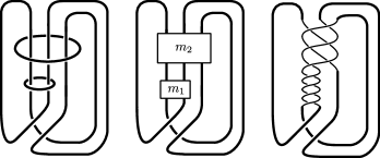
Figure 1. Left: The seed link $K$ and the 2-fusion knot $K(m_{1},m_{2})$. As an example $K(2,1)$ is the $(-2,3,7)$ pretzel knot.

The 2-parameter family of 2-fusion knots includes the 2-strand torus knots, the $(-2,3,p)$ pretzel knots and some knots that appear in the work of Gordon-Wu related to exceptional Dehn surgery [GW08]. The non-Montesinos, non-alternating knot $K(-1,3)=K4_{3}$ was the focus of [GL05a] regarding a numerical confirmation of the volume conjecture. The topology and geometry of 2-fusion knots is explained in detail in Section 5.3.

1.5. Our results

Our main Theorem 1.1 gives an explicit formula for the Jones slope for all 2-fusion knots $K(m_{1},m_{2})$. Recall that the Jones slope(s) $js_{K}$ of a knot $K$ is the set of values of the periodic function $c_{K,2}:\mathbb{N}\to\mathbb{Q}$ that governs the leading order of the $q$-degree of $J_{K,n}(q)$. In our case set of Jones slopes is a singleton for each pair $m_{1},m_{2}$ so we denote by $\mathrm{js}(m_{1},m_{2})\in\mathbb{Q}$ the unique element of the set of Jones slopes of $K(m_{1},m_{2})$. The formula for $\mathrm{js}$ is a piece-wise rational function of $m_{1},m_{2}$ defined on the lattice points $\mathbb{Z}^{2}$ of the plane, which are partitioned into five sectors shown in color-coded fashion in Figure 2. The reader may observe that the 5 branches of the function $\mathrm{js}:\mathbb{Z}^{2}\to\mathbb{Q}$ do not agree when extrapolated. For example for $m_{1}<1$ and $m_{2}=0$ the formula $2m_{2}+\frac{1}{2}$ from the red region does not agree (when extrapolated) with the actual value $0$ for the Jones slope at $m_{2}=0$. This disagreement disappears when we study the corresponding real optimization problem in Section 4 below. The branches given there actually fit together continuously.

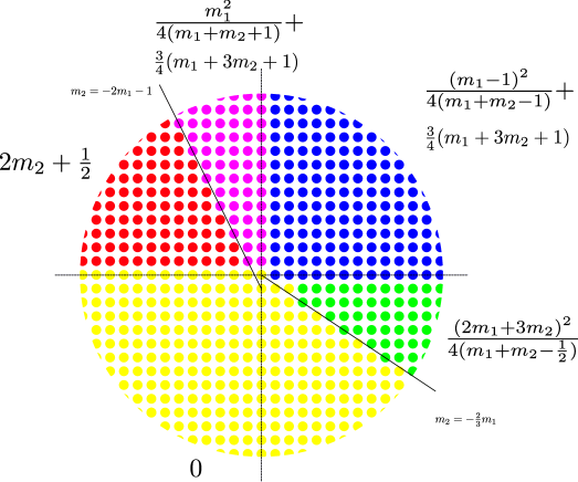
Figure 2. The formula for the Jones slope of $K(m_{1},m_{2})$.

Theorem 1.1.

For any $m_{1},m_{2}$ there is only one Jones slope. Moreover, if we divide the $(m_{1},m_{2})$-plane into regions as shown in Figure 2 then the Jones slope $\mathrm{js}(m_{1},m_{2})$ of $K(m_{1},m_{2})$ is given by:

(5) $$\mathrm{js}(m_{1},m_{2})=\begin{cases}\frac{(m_{1}-1)^{2}}{4(m_{1}+m_{2}-1)}+\frac{3m_{1}+9m_{2}+3}{4}&\text{if}\,\,m_{1}\geq 1,\,\,m_{2}\geq 0\\ \frac{m_{1}^{2}}{4(m_{1}+m_{2}+1)}+\frac{3m_{1}+9m_{2}+3}{4}&\text{if}\,\,m_{1}\leq 0,\,\,m_{2}\geq-1-2m_{1},\,\,m_{2}\geq 1\\ 2m_{2}+\frac{1}{2}&\text{if}\,\,0<m_{2},\,\,m_{2}<-1-2m_{1}\\ 0&\text{if}\,\,m_{2}\leq 0,\,\,m_{2}\leq-\frac{2}{3}m_{1},\,\,\text{or}\,\,(m_{1},m_{2})=(2,-1)\\ \frac{(2m_{1}+3m_{2})^{2}}{4(m_{1}+m_{2}-\frac{1}{2})}&\text{if}\,\,m_{2}>-\frac{2}{3}m_{1},\,\,m_{2}\leq-1\end{cases}$$

with $\mathrm{js}(1,0)=3/2$.

Combining the work of [DG12, Thm.1.9] we obtain a proof for the slope conjecture for a large class of $2$-fusion knots.

Corollary 1.2.

The slope conjecture is true for all 2-fusion knots $K(m_{1},m_{2})$ with $m_{1}>1,m_{2}>0$.

As the knots are generally non-Montesinos this result is beyond the reach of other known techniques. Also the Jones slopes are of great interest in that they are generally not integers so that they can not be found using semi-adequacy.

We should remark that the incompressibility criterion of [DG12] can also be applied to prove the slope conjecture for the remaining $2$-fusion knots. However, this is not the focus of the present paper, and we will not provide any further details on this separate matter.

Remark 1.3.

Using the involution

(6) $$K(m_{1},m_{2})=-K(1-m_{1},-1-m_{2}),\qquad K(-1,m_{2})=K(-1,-m_{2})$$

Theorem 1.1 computes the Jones slopes of the mirror of the family of 2-fusion knots. Hence, for every 2-fusion knot, we obtain two Jones slopes.

Remark 1.4.

The proof of Theorem 1.1 also gives a formula for the degree of the colored Jones polynomial. This formula is valid for all $n$, and it is manifestly a quadratic quasi-polynomial. See Section 4.

Remark 1.5.

Theorem 1.1 has a companion Theorem 4.2 which is the solution to a real quadratic optimization problem. Theorem 4.1 implies the existence of a function $\mathrm{js}_{\mathbb{R}}:\mathbb{R}^{2}\to\mathbb{R}$ with the following properties:

• $\mathrm{js}_{\mathbb{R}}$ is continuous and piece-wise rational, with corner locus (i.e., locus of points where $\mathrm{js}_{\mathbb{R}}$ is not differentiable) given by quadratic equalities and inequalities whose complement divides the plane $\mathbb{R}^{2}$ into 9 sectors, shown in Figure 5.

• $\mathrm{js}_{\mathbb{R}}$ is a real interpolation of $\mathrm{js}$ in the sense that it satisfies

  $$\mathrm{js}_{\mathbb{R}}(m_{1},m_{2})=\mathrm{js}(m_{1},m_{2})$$

  for all integers $m_{1},m_{2}$ except those of the form $(m_{1},0)$ with $m_{1}\leq 0$ and $(2,-1)$. See Corollary 4.3 below.

• Each of the 9 branches of $\mathrm{js}_{\mathbb{R}}$ (after multiplication by 4) becomes a boundary slope of $K(m_{1},m_{2})$ valid in the corresponding region, detected by the incompressibility criterion of [DG12, Sec.8].

2. The colored Jones polynomial of 2-fusion knots

2.1. A state sum for the colored Jones polynomial

The cut-and-paste axioms of TQFT allow to compute the quantum invariants of knotted objects in terms of a few building blocks, using a combinatorial presentation of the knotted objects. In our case, we are interested in state sum formulas for the colored Jones function $J_{K,n}(q)$ of a knot $K$. Of the several state sum formulas available in the literature, we will use the fusion formulas that appear in [CFS95, Cos09, MV94, GvdV12, KL94, Tur88]. Fusion of knots are knotted trivalent graphs. There are five building blocks of fusion (the functions $\mu,\nu,\mathrm{U},\Theta,\mathrm{Tet}$ below), expressed in terms of quantum factorials. Recall the quantum integer $[n]$ and the quantum factorial $[n]!$ of a natural number $n$ are defined by

$$[n]=\frac{q^{n/2}-q^{-n/2}}{q^{1/2}-q^{-1/2}},\qquad[n]!=\prod_{k=1}^{n}[k]!$$

with the convention that $[0]!=1$. Let

$$\genfrac{[}{]}{0.0pt}{}{a}{a_{1},a_{2},\dots,a_{r}}=\frac{[a]!}{[a_{1}]!\dots[a_{r}]!}$$

denote the multinomial coefficient of natural numbers $a_{i}$ such that $a_{1}+\dots a_{r}=a$. We say that a triple $(a,b,c)$ of natural numbers is admissible if $a+b+c$ is even and the triangle inequalities hold. In the formulas below, we use the following basic trivalent graphs $\mathrm{U},\Theta,\mathrm{Tet}$ colored by one, three and six natural numbers (one in each edge of the corresponding graph) such that the colors at every vertex form an admissible triple shown in Figure 2.1.

Let us define the following functions.

$$\mu(a) = (-1)^{a}q^{\frac{-a(a+2)}{4}}$$

$$\nu(c,a,b) = (-1)^{\frac{a+b-c}{2}}q^{\frac{a(a+2)+b(b+2)-c(c+2)}{8}}$$

$$\mathrm{U}(a) = (-1)^{a}[a+1]$$

$$\Theta(a,b,c) = (-1)^{\frac{a+b+c}{2}}[\frac{a+b+c}{2}+1]\genfrac{[}{]}{0.0pt}{}{\frac{a+b+c}{2}}{\frac{-a+b+c}{2},\frac{a-b+c}{2},\frac{a+b-c}{2}}$$

$$\mathrm{Tet}(a,b,c,d,e,f) = \sum_{k=\max T_{i}}^{\min S_{j}}(-1)^{k}[k+1]\genfrac{[}{]}{0.0pt}{}{k}{S_{1}-k,S_{2}-k,S_{3}-k,k-T_{1},k-T_{2},k-T_{3},k-T_{4}}$$

where

(7) $$S_{1}=\frac{1}{2}(a+d+b+c)\qquad S_{2}=\frac{1}{2}(a+d+e+f)\qquad S_{3}=\frac{1}{2}(b+c+e+f)$$

(8) $$T_{1}=\frac{1}{2}(a+b+e)\qquad T_{2}=\frac{1}{2}(a+c+f)\qquad T_{3}=\frac{1}{2}(c+d+e)\qquad T_{4}=\frac{1}{2}(b+d+f).$$

An assembly of the five building blocks can compute the colored Jones function of any knot. The next theorem is an exercise in fusion following word for word the proof of [GL05a, Thm.1]. An elementary and self-contained introduction to fusion is available in [GL05a, Sec.3.2]. In particular, the calculation of the colored Jones polynomial of the $2$-fusion knot $K(-1,3)$ (generalized verbatim to all $2$-fusion knots) is given in [GL05a, Sec.3.3, p.390].

Consider the function

$$S(m_{1},m_{2},n_{,}k_{1},k_{2})(q) = \frac{\mu(n)^{-w(m_{1},m_{2})}}{\mathrm{U}(n)}\nu(2k_{1},n,n)^{2m_{1}+2m_{2}}\nu(n+2k_{2},2k_{1},n)^{2m_{2}+1}$$

$$\cdot\frac{\mathrm{U}(2k_{1})\mathrm{U}(n+2k_{2})}{\Theta(n,n,2k_{1})\Theta(n,2k_{1},n+2k_{2})}\mathrm{Tet}(n,2k_{1},2k_{1},n,n,n+2k_{2})\,.$$

Theorem 2.1.

For every $m_{1},m_{2}\in\mathbb{Z}$ and $n\in\mathbb{N}$, we have:

(10) $$J_{K(m_{1},m_{2}),n}(q)=\sum_{(k_{1},k_{2})\in nP\cap\mathbb{Z}^{2}}S(m_{1},m_{2},n_{,}k_{1},k_{2})(q)\,,$$

where $P$ is the polytope from Figure 3 and the writhe of $K(m_{1},m_{2})$ is given by $w(m_{1},m_{2})=2m_{1}+6m_{2}+2$.

Figure 3. The polygon $P$ on the left and its decomposition into three regions $P_{1},P_{2},P_{3}$ on the right.

Remark 2.2.

Notice that for every $n\in\mathbb{N}$, we have:

$$\{(k_{1},k_{2})\in\mathbb{Z}^{2}\,\,|0\leq 2k_{1}\leq 2n,\quad|n-2k_{1}|\leq n+2k_{2}\leq n+2k_{1}\}=nP\cap\mathbb{Z}^{2}.$$

For the purpose of visualization, we show the lattice points in $4P$ and $5P$ in Figure 4.

Figure 4. The lattice points in $4P$ and $5P$.

2.2. The leading term of the building blocks

In this section we compute the leading term of the five building blocks of our state sum.

Definition 2.3.

If $f(q)\in\mathbb{Q}(q^{1/4})$ is a rational function, let $\delta(f)$ and $\mathrm{lt}(f)$ the minimal degree and the leading coefficient of the Laurent expansion of $f(q)\in\mathbb{Q}((q^{1/4}))$ with respect to $q^{1/4}$. Let

(11) $$\widehat{f}(q)=\mathrm{lt}(f)q^{\delta(f)}$$

denote the leading term of $f(q)$.

We may call $\widehat{f}(q)$ the tropicalization of $f(q)$. Observe the trivial but useful identity:

(12) $$\widehat{fg}=\hat{f}\,\hat{g}$$

for nonzero functions $f,g$.

Lemma 2.4.

For all admissible colorings we have:

$$\mathrm{lt}(\mu)(a) = (-1)^{a}$$

$$\mathrm{lt}(\nu)(c,a,b) = (-1)^{\frac{a+b-c}{2}}$$

$$\mathrm{lt}(\mathrm{U})(a) = (-1)^{a}$$

$$\mathrm{lt}(\Theta)(a,b,c) = (-1)^{\frac{a+b+c}{2}}$$

$$\mathrm{lt}(\mathrm{Tet})(a,b,c,d,e,f) = (-1)^{k^{*}}$$

where

$$k^{*}=\min S_{j}$$

and

$$\delta(\mu)(a) = \frac{-a(a+2)}{4}$$

$$\delta(\nu)(c,a,b) = \frac{a(a+2)+b(b+2)-c(c+2)}{8}$$

$$\delta(\mathrm{U})(a) = \frac{a}{2}$$

$$\delta(\Theta)(a,b,c) = -\frac{1}{8}(a^{2}+b^{2}+c^{2})+\frac{1}{4}(ab+ac+bc)+\frac{1}{4}(a+b+c)$$

$$\delta(\mathrm{Tet})(a,b,c,d,e,f) = \delta(b_{7})(S_{1}-k^{*},S_{2}-k^{*},S_{3}-k^{*},k^{*}-T_{1},k^{*}-T_{2},k^{*}-T_{3},k^{*}-T_{4})+\frac{k^{*}}{2}$$

where $S_{j}$ and $T_{i}$ are given in Equations (7) and (8), $b_{7}(a_{1},\dots,a_{7})=\genfrac{[}{]}{0.0pt}{}{a}{a_{1},a_{2},\dots,a_{7}}$ is the 7-binomial coefficient and

$$\delta(b_{7})(a_{1},\dots,a_{7}) = \frac{1}{4}\left(\left(\sum_{i=1}^{7}a_{i}\right)^{2}-\sum_{i=1}^{7}a_{i}^{2}\right).$$

Proof.

Use the fact that

$$\widehat{[a]}=q^{\frac{a-1}{2}}$$

and

$$\widehat{[a]!}=q^{\frac{a^{2}-a}{4}}$$

This computes the leading term of $\Theta$ and of the quantum multinomial coefficients. Now $\mathrm{Tet}(a,b,c,d,e,f)$ is given by a 1-dimensional sum of a variable $k$. It is easy to see that the leading term comes the maximum value $k^{*}$ of $k$. The result follows. ∎

2.3. The leading term of the summand

Consider the function $Q$ defined by

$$Q(m_{1},m_{2},n,k_{1},k_{2}) = \frac{k_{1}}{2}-\frac{3k_{1}^{2}}{2}-3k_{1}k_{2}-k_{2}^{2}-k_{1}m_{1}-k_{1}^{2}m_{1}-k_{2}m_{2}-k_{2}^{2}m_{2}-6k_{1}n$$

$$-3k_{2}n+2m_{1}n+4m_{2}n-k_{2}m_{2}n-2n^{2}+m_{1}n^{2}+2m_{2}n^{2}$$

$$+\frac{1}{2}\left((1+8k_{1}+4k_{2}+8n)\min\{l_{1},l_{2},l_{3}\}-3\min\{l_{1},l_{2},l_{3}\}^{2}\right)$$

where

$$l_{1}=2k_{1}+n,\qquad l_{2}=2k_{1}+k_{2}+n,\qquad l_{3}=k_{2}+2n.$$

Notice that for fixed $m_{1},m_{2}$ and $n$, the function $k=(k_{1},k_{2})\mapsto Q(m_{1},m_{2},n,k)$ is piece-wise quadratic function. Moreover, for all $m_{1},m_{2}$ and $n$ the restriction of the above function to each region of $nP$ is a quadratic function of $(k_{1},k_{2})$.

Lemma 2.5.

For all $(m_{1},m_{2},n_{,}k_{1},k_{2})$ admissible, we have

$$\hat{S}(m_{1},m_{2},n_{,}k_{1},k_{2})=(-1)^{k_{1}+n+\min\{2k_{1},2k_{1}+k_{2},k_{2}+n\}}q^{Q(m_{1},m_{2},n_{,}k_{1},k_{2})}$$

Proof.

It follows easily from Section 2.2 and Equation (12). ∎

3. Proof of Theorem 1.1

The proof involves four cases:

Case 0	Case 1	Case 2	Case 3
$m_{2}\in\{0,-1\}$	$m_{1},m_{2}\geq 1$	$m_{1}\leq 0,m_{2}\geq 1$	$m_{2}\leq-2$

Case $0$ involves only alternating torus knots since $K(m_{1},0)=T(2,2m_{1}+1)$ and $K(m_{1},-1)=T(2,2m_{1}-3)$ for which the Jones slopes were already known [Gar11b].

In the remaining three cases we will take the following steps:

1. Estimate partial derivatives of $Q$ in the various regions $P_{i}$ to narrow down the location of the lattice points that achieve the maximum of $Q$ on $nP\cap\mathbb{Z}^{2}$. In all cases they will be on a single boundary line of $Q$.

2. Since the restriction of $Q$ to a boundary line is an explicit quadratic function in one variable, there can be at most $2$ maximizers and we can readily compute them.

3. If there are two maximizers, compute the leading term of the corresponding summand to see if they cancel out.

4. If there is no cancellation, then we can evaluate $Q(m_{1},m_{2},n,k)/n^{2}$ at either of the maximizers $k$ to get the slope.

5. If there is cancellation we first have to explicitly take together all the canceling terms until no more cancellation occurs at the top degree. This happens only in the difficult Case 3.

3.1. Case 1: $m_{1},m_{2}\geq 1$

Recall that $Q_{i}$ is $Q$ restricted to the region $nP_{i}$ defined in Figure 3. We have:

(14) $$\frac{\partial Q_{1}}{\partial k_{2}}<0\qquad\frac{\partial Q_{2}}{\partial k_{1}},\frac{\partial Q_{2}}{\partial k_{2}}<0\qquad\frac{\partial Q_{3}}{\partial k_{2}}<0\,.$$

Before we may conclude that the maximum of $Q$ on $nP\cap\mathbb{Z}^{2}$ is on the line $k_{2}=-k_{1}$ we have to check the following. For odd $n$ there could be a jump across the line $k=\frac{n}{2}$ between regions $nP_{2}$ and $nP_{1}$. We therefore set $n=2N+1$ explicitly check that

$$Q_{1}(m_{1},m_{2},2N+1,N,-N)-Q_{2}(m_{1},m_{2},2N+1,N+1,-N)>0$$

Restricted to the line $k_{2}=-k_{1}$, $Q$ is a negative definite quadratic in $k_{1}$ with critical point

$$c_{1}=\frac{1-m_{1}+m_{2}+m_{2}n}{2(-1+m_{1}+m_{2})}$$

For $m_{1}>1$ we have $c_{1}\in(-\frac{1}{2},\frac{n}{2}]$ and for $m_{1}=1$ we have $c_{1}=\frac{n+1}{2}$. In both cases the maximizers are the lattice points in the diagonal closest to $c_{1}$ satisfying $k_{1}\leq\frac{n}{2}$. There may be a tie for the maximum between two adjacent points. To rule out the possibility of cancellation we take a look at the leading term restricted to the line $k_{2}=-k_{1}$. The leading term is $(-1)^{n}$. Since the sign of the leading term is independent of $k_{1}$ along the diagonal, there cannot be cancellation. We may conclude that the slope is given by the constant term of $Q(m_{1},m_{2},n,c_{1},-c_{1})/n^{2}$. This gives the slope $\frac{(m_{1}-1)^{2}}{4(m_{1}+m_{2}-1)}+\frac{m_{1}+9m_{2}+1}{4}$ indicated in the blue region of Figure 2.

3.2. Case 2: $m_{1}\leq 0,m_{2}\geq 1$

We have:

(15) $$\frac{\partial Q_{1}}{\partial k_{1}}>0,\frac{\partial Q_{1}}{\partial k_{2}}<0\qquad\frac{\partial Q_{2}}{\partial k_{2}}<0\qquad\frac{\partial Q_{3}}{\partial k_{2}}<0\,.$$

Before we may conclude that the maximum of $Q$ on $nP\cap\mathbb{Z}^{2}$ is on the line $k_{2}=k_{1}-n$ we have to check the following. For odd $n$ there could be a jump across the line $k_{1}=\frac{n}{2}$ between regions $nP_{2}$ and $nP_{1}$. We therefore set $n=2N+1$ explicitly check that

$$Q_{2}(m_{1},m_{2},2N+1,N+1,-N)-Q_{1}(m_{1},m_{2},2N+1,N,-N)>0$$

Restricted to the line $k_{2}=k_{1}-n$ the coefficient of $k_{1}^{2}$ in $Q$ is $a=-1-m_{1}-m_{2}$. If $a>0$ the critical point $c_{2}$ is given by

$$c_{2}=\frac{1-m_{1}+m_{2}+m_{2}n}{2(-1+m_{1}+m_{2})}$$

Since $c_{2}<\frac{3}{4}n$ the maximizer is given by $k_{1}=n$ and so the slope is: $2m_{2}+\frac{1}{2}$ as shown in red in Figure 2. If $a=0$ we have the same conclusion because along the diagonal $Q$ is now an increasing linear function in $k_{1}$. Finally if $a<0$ we need to determine if $c_{2}\in[\frac{n}{2}-\frac{1}{2},n+\frac{1}{2}]$.

We always have $c_{2}>\frac{n-1}{2}$, and if in addition $1+2m_{1}+m_{2}<0$ then $c_{2}>n-1/2$. This means the maximizer is $k_{1}=n$ and the slope is $\frac{1}{2}+2m_{2}$ as shown in red in Figure 2.

If $1+2m_{1}+m_{2}\geq 0$ then $c_{2}\in[\frac{n-1}{2},n+\frac{1}{2}]$ and the maximizers are the lattice points on the line closest to $c_{2}$. There may of course be cancellation if there is a tie. To rule this out we check that along the line the sign of the leading term is independent of $k_{1}$. Indeed the leading term on this line is $(-1)^{n}$.

We may conclude that the slope is given by the constant term of $Q(m_{1},m_{2},n,c_{2},c_{2}-n)/n^{2}$ This gives the slope $\frac{m_{1}^{2}}{4(m_{1}+m_{2}+1)}+\frac{m_{1}+9m_{2}+1}{4}$ indicated in the purple region of Figure 2.

3.3. Case 3: $m_{1}\leq 0,m_{2}\leq-2$

One can check that:

(16) $$\frac{\partial Q_{1}}{\partial k_{2}}>0\qquad\frac{\partial Q_{2}}{\partial k_{2}}>0\qquad\frac{\partial Q_{3}}{\partial k_{2}}>0\,.$$

This means that the lattice maximizers of $Q$ will be on the diagonal $k_{1}=k_{2}$. Here the restriction of $Q$ is a quadratic and the coefficient of $k_{1}^{2}$ is $\frac{1}{2}-m_{1}-m_{2}$. If $m_{1}\leq-m_{2}$ then it is positive definite with critical point given by

$$c_{3}=\frac{-3+2m_{1}+2m_{2}+2n+2m_{2}n}{2(1-2m_{1}-2m_{2})}$$

We have $c_{3}<0$ so the maximum is attained at $k_{1}=n$ giving a slope of $0$ as shown in yellow in Figure 2.

If $m_{1}>-m_{2}$ the quadratic $Q$ is negative definite on the diagonal and the critical point $c_{3}$ satisfies $c_{3}>-\frac{1}{2}$. Furthermore $c_{3}\geq n-\frac{1}{2}$ if and only if $-3m_{2}\geq 2m_{1}$ and this case we get again the maximizer $k_{1}=n$ and slope $0$.

The only remaining case is $2m_{1}>-3m_{2}$, which means $c_{3}\in(-\frac{1}{2},n-\frac{1}{2}]$. Here we have to check for cancellation and indeed, there will be cancellation along a subsequence since the leading term alternates along the diagonal, it is $(-1)^{k_{1}+n}$.

To finish the proof we must rule out the possibility of a new slope occurring when the degree drops dramatically due to cancellation. Below we will deal with the cancellation and show the drop in degree is at most linear in $n$ so that no new slope can appear. Our conclusion then is that the slope is given by the constant term of $Q_{3}(m_{1},m_{2},n,c_{3},c_{3})/n^{2}$ which is: $\frac{(2m_{1}+3m_{2})^{2}}{4(m_{1}+m_{2}-\frac{1}{2})}$ as shown in green in Figure 2.

3.4. Analysis of the cancellation in Case 3

Cancellation happens exactly when the critical point on the diagonal is a half integer $c_{3}\in\frac{1}{2}+\mathbb{Z}$. Note also that not just the two terms tying for the maximum cancel out. All the terms along the diagonal corresponding to $k_{1}=c_{3}\pm\frac{2b+1}{2}$ cancel out to some extent. Here $b=0\ldots\min(c_{3},n-c_{3})-\frac{1}{2}$.

Along the diagonal the Tet consists of a single term so that the summand $S$ simplifies considerably, call it $D$:

$$D(k):=S(m_{1},m_{2},n,k,k) =(-1)^{(2m_{2}+1)n/2+n}q^{-(2m_{2}+1)n^{2}/8}[n]!\times$$

$$\quad(-1)^{k}q^{-(m_{1}+m_{2})k(k+1)-(2m_{2}+1)n(2k+1)/4}\frac{[n+2k+1][2k+1]!}{[k]![n+k+1]!}$$

To see how far the degree drops when taking together the canceling terms in pairs and take together $D(k)$ and $D(k-a)$. For $a\in\mathbb{N}$ the result is:

$$D(k)+D(k-a) =C\left(q^{\alpha}\{n+2k-2a+1\}\frac{\{k\}!\{n+k+1\}!}{\{k-a\}!\{n+k-a+1\}!}\right.$$

$$\quad+\left.(-1)^{s}q^{\beta}\{n+2k+1\}\frac{\{2k+1\}!}{\{2k-2a+1\}!}\right)\,.$$

Here $C$ is an irrelevant common factor and in case of cancellation the monomials $q^{\alpha}$ and $(1)^{s}q^{\beta}$ are determined to make the leading terms of equal degree and opposite sign. Lastly we have taken out all denominators of the quantum numbers and factorials and define $\{k\}=[k](q^{\frac{1}{2}}-q^{-\frac{1}{2}})$.

Since we assume the leading terms cancel we investigate the next degree term in both parts of the above formula. For this we can ignore $C$ and the monomials and restrict ourselves to the two products of terms of the form $\{x\}$. Both products can be simplified to remove the denominator. The difference in degree between the two terms of $\{x\}$ is exactly $x$. If $\{x\}$ is the least integer that occurs in the product then the difference in degree between the leading term and the highest subleading term is exactly $x$. For the first term $x$ is $k-a+1$ and for the second term it is $x=2k-2a+2$. In conclusion the highest subleading term does not cancel out and has degree exactly $k-a+1$ lower than the leading term.

To finish the argument we would like to show that the $b=0$ terms $k_{1}=c_{3}\pm\frac{1}{2}$ still produce the highest degree term after cancellation. This is not obvious since the degree drops by exactly $c_{3}-b+\frac{1}{2}$. In other words after cancellation the degree of the terms corresponding to $b$ gains exactly $b$ relative to the $b=0$ terms. To settle this matter we show that the difference in degree before cancellation was more than $b$.

$$Q_{3}(m_{1},m_{2},n,c_{3}+\frac{1}{2},c_{3}+\frac{1}{2})-Q_{3}(m_{1},m_{2},n,c_{3}-b-\frac{1}{2},c_{3}-b-\frac{1}{2})=\frac{b(1+b)}{2}(-1+2m_{1}+2m_{2})>b$$

Because $b\geq 1$ and $2m_{1}>-3m_{2}$ so $-1+2m_{1}+2m_{2}>-1-m_{2}\geq 1$.

The same computation also shows how to deal with the diagonal terms where $b>\min(c_{3},n-c_{3})-\frac{1}{2}$ that did not suffer any cancellation because their symmetric partner was outside of $nP$. We need to show that the difference in degree before cancellation is at least $c_{3}+\frac{1}{2}$. So for $b=\min(c_{3},n-c_{3})-\frac{1}{2}$ check explicitly that $\frac{b(1+b)}{2}(-1+2m_{1}+2m_{2})>c_{3}+\frac{1}{2}$. This is true provided that $n>m_{1}$.

Finally we check that the degree of the $b=0$ terms before cancellation is greater than $c_{3}+\frac{1}{2}$ plus the degree of any off-diagonal term. For this we only need to consider the terms $(k_{1},k_{2})=(k_{1},k_{1}-1)$. Again it follows by a routine computation.

4. Real versus lattice quadratic optimization

4.1. Real quadratic optimization with parameters

In this section we study the real quadratic optimization problem of Equation (4) and compare it with the lattice quadratic optimization problem of Theorem 1.1.

Fix a rational convex polytope $P$ in $\mathbb{R}^{r}$ and a piece-wise quadratic function $\delta$ in the variables $n,x$ where $x=(x_{1},\dots,x_{r})$. Then, we have:

$$\hat{\delta}_{\mathbb{R}}(n):=\max\{\delta(n,x)\,\,|\,\,x\in nP\}=\max\{\delta(n,nx)\,\,|\,\,x\in P\}\,.$$

Observe that $\delta(n,nx)$ is a quadratic polynomial in $n$ with coefficients piece-wise quadratic polynomial in $x$. it follows that for $n$ large enough, $\hat{\delta}_{\mathbb{R}}(n)$ is given by a quadratic polynomial in $n$. If $\mathrm{js}_{\mathbb{R}}$ denote the coefficient of $n^{2}$ in $\hat{\delta}_{\mathbb{R}}(n)$, and $\delta_{2}(x)$ denotes the coefficient of $n^{2}$ in $\delta(n,nx)$ then we have:

$$\mathrm{js}_{\mathbb{R}}=\max\{\delta_{2}(x)\,\,|\,\,x\in P\}\,.$$

If $\delta$ depends on some additional parameters $m\in\mathbb{R}^{r}$, then we get a function

(17) $$\mathrm{js}_{\mathbb{R}}:\mathbb{R}^{r}\mapsto\mathbb{R}\,.$$

Assume that dependence of $\delta$ on $m$ is polynomial with real coefficients. To compute $\mathrm{js}_{\mathbb{R}}(m)$, consider the piece-wise quadratic polynomial (in the $x$ variable) $\delta_{2}(m,x)$, which achieves a maximum at some point of the compact set $P$. Subdividing $P$ if necessary, we may assume that $\delta_{2}(m,x)$ is a polynomial in $x$. If the maximum $\hat{x}$ is at the interior of $P$, since $\delta_{2}(m,x)$ is quadratic, its gradient is an affine linear function of $x$, hence it has a unique zero. In that case, it follows that $\hat{x}$ is the unique critical point of $\delta_{2}(m,x)$ and $\delta_{2}(m,x)$ has negative definite quadratic part. Since the coefficients of the quadratic function $\delta_{2}(m,x)$ of $x$ are polynomials in $m$, it follows that in the above case the coefficients of $\hat{x}$ are rational functions of $m$. The condition that $\hat{x}$ is a maximum point in the interior of $P$ can be expressed by polynomial equalities and inequalities on $m$. This defines a semi-algebraic set [BPR03]. On the other hand, if $\hat{x}$ lies in the boundary of $P$, then either $\hat{x}$ is a vertex of $P$ or there exists a face $F$ of $P$ such that $\hat{x}$ lies in the relative interior of $F$. Restricting $\delta_{2}(m,x)$ and using induction on $r$, or evaluating at $\hat{x}$ a vertex of $P$ implies the following.

Theorem 4.1.

With the above assumptions, $\mathrm{js}_{\mathbb{R}}:\mathbb{R}^{r}\mapsto\mathbb{R}$ is a piece-wise rational function of $m$, defined on finitely many sectors whose corner locus is a closed semi-algebraic set of dimension at most $r-1$. Moreover, $\mathrm{js}_{\mathbb{R}}$ is continuous.

Recall that the corner locus of a piece-wise function on $\mathbb{R}^{r}$ is the set of points where the function is not differentiable. Note that the proof of Theorem 4.1 is constructive, and easier than the corresponding lattice optimization problem, since we do not have to worry about ties. Moreover, since we are doing doing a sum, we do not have to worry about cancellations.

4.2. The case of $2$-fusion knots

We now illustrate Theorem 4.1 for the case of $2$-fusion knots, where $\delta(m_{1},m_{2},n,x_{1},x_{2})$ is given by Equation (2.3). Notice that $\delta(m,n,x)$ is an affine linear function of $m=(m_{1},m_{2})\in\mathbb{R}^{2}$. A case analysis (similar but easier than the one of Section 3 shows the following.

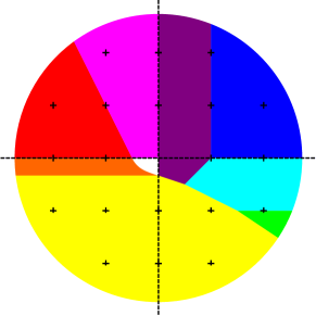
Figure 5. The nine regions of $\mathrm{js}_{\mathbb{R}}$ of Theorem 4.2.

Define $\mathrm{js}_{\mathbb{R}}(m_{1},m_{2})$ to be the real maximum of the summand for the fusion state sum of $K(m_{1},m_{2})$.

Theorem 4.2.

If we divide the $(m_{1},m_{2})$-plane into regions as shown in Figure 5 then $\mathrm{js}_{\mathbb{R}}(m_{1},m_{2})$ is given by:

$$\mathrm{js}_{\mathbb{R}}(m_{1},m_{2})=$$

(18) $$\begin{cases}\frac{(m_{1}-1)^{2}}{4(m_{1}+m_{2}-1)}+\frac{3m_{1}+9m_{2}+3}{4}&\text{if}\,\,m_{1}>1,\,\,m_{2}\geq 0\\ \frac{3m_{1}+9m_{2}+3}{4}&\text{if}\,\,0\leq m_{1}\leq 1,\,\,1+m_{1}+3m_{2}\geq 0,\,\,1-m_{1}+m_{2}\geq 0\\ \frac{m_{1}^{2}}{4(m_{1}+m_{2}+1)}+\frac{3m_{1}+9m_{2}+3}{4}&\text{if}\,\,m_{1}\leq 0,\,\,m_{2}\geq 0,\,\,m_{2}\geq-1-2m_{1}\\ 2m_{2}+\frac{1}{2}&\text{if}\,\,m_{2}>0,\,\,1+2m_{1}+m_{2}\geq 0\\ \frac{(3m_{2}+1)^{2}}{4(m_{2}+\frac{1}{2})}&\text{if}\,\,-\frac{1}{3}\leq m_{2}\leq 0,\,\,1+2m_{1}+3m_{2}+4m_{1}m_{2}\leq 0\\ 0&\text{if}\,\,m_{2}\leq-\frac{1}{3},\,\,1+m_{1}+3m_{2}\leq 0,\,\,1+2m_{1}+4m_{2}\leq 0,\,\,m_{2}\leq-\frac{2}{3}m_{1}\\ \frac{(2m_{1}+3m_{2})^{2}}{4(m_{1}+m_{2}-\frac{1}{2})}&\text{if}\,\,m_{2}>-\frac{2}{3}m_{1},\,\,m_{2}\leq-1\\ m_{1}+2m_{2}+\frac{1}{2}&\text{if}\,\,-1\leq m_{2}\leq 0,\,\,1-m_{1}+m_{2}\leq 0,\,\,1+2m_{1}+4m_{2}\geq 0\\ I(m_{1},m_{2})&\text{if}\,\,1+2m_{1}+3m_{2}+4m_{1}m_{2}\geq 0,\,\,-\frac{1}{2}\leq m_{1}\leq 0,\,\,-\frac{1}{3}\leq m_{2}\leq 0\end{cases}$$

where

$$I(m_{1},m_{2})=\frac{3+6m_{1}+4m_{1}^{2}+18m_{2}+24m_{1}m_{2}+8m_{1}^{2}m_{2}+27m_{2}^{2}+18m_{1}m_{2}^{2}}{4(1+m_{1}+3m_{2}+2m_{1}m_{2})}$$

Corollary 4.3.

An comparison between Theorems 1.1 and 4.2 reveals that $\mathrm{js}(m_{1},m_{2})=\mathrm{js}_{\mathbb{R}}(m_{1},m_{2})$ for all pairs of integers $(m_{1},m_{2})\in\mathbb{Z}^{2}$ except those of the form $(m_{1},0)$ with $m_{1}\leq 0$ and $(2,-1)$. For these exceptional pairs, $K(m_{1},m_{2})$ is a torus knot.

5. $k$-seed links and $k$-fusion knots

5.1. Seeds and fusion

There are several ways to tabulate and classify knots, and among them

• by crossing number as was done by Rolfsen [Rol90],

• by the number of ideal tetrahedra (for hyperbolic knots) as is the standard in hyperbolic geometry [Thu77, CDW],

• by arborescent planar projections, studied by Conway and Bonahon-Siebenmann [Cos09, BS11],

• by fusion [Thu02],

• by shadows [Tur92].

Here we review the fusion construction of knots (and more generally, knotted trivalent graphs) which originates from cut and paste axioms in quantum topology. The construction was introduced by Bar-Natan and Thurston, appeared in [Thu02] and further studied by the second author [vdV09]. Our definition of fusion is reminiscent to W. Thurston’s hyperbolic Dehn filling [Thu77], and differs from a construction of knots by the same name (fusion) that appears in Kawauchi’s book [Kaw96, p.171].

Figure 6. The moves $A$,$U$,$X$ and the theta graph (upper right).

Definition 5.1.

A seed link is a link that can be produced from the theta graph by applying the moves $A,U,X$ shown in figure 6. The additional components created by $U$ and $X$ are called belts. A $k$-seed link is a seed link with $k$ belts.

Note that the sign of the crossing introduced by the $X$-move is does not affect the complement of the seed link. If desired we may always perform all the $A$ moves first.

Definition 5.2.

Let $L$ be a $k$-seed link together with an ordering of its belts. Define the $k$-fusion link $L(m_{1},\ldots,m_{k})$ to be the link obtained by $-\frac{1}{m_{j}}$ Dehn filling on the $j$-th belt of $L$ for all $j=1,\dots,k$.

Recall that the result of $-1/m$ Dehn filling along an unknot $C$ which bounds a disk $D$ replaces a string that meets $D$ with $m$ full twists, right-handed if $m>0$ and left-handed if $m<0$; see Figure 7 and [Kir78].

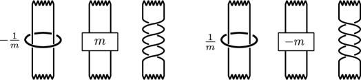
Figure 7. The effect of Dehn filling on a link. In the picture we have taken $m=2$.

In a picture of a seed link the belts will always be enumerated from bottom to top. So for example the first belt of $K$ is the smallest one.

As suggested above, fusion is not just a way to produce a special class of knots. All knots and links can be presented this way although not in a unique way.

Theorem 5.3.

Any link is a $k$-fusion link for some $k$. The number of fusions is at most the number of twist regions of a diagram.

This theorem has its roots in Turaev’s theory of shadows. A self-contained proof can be found in [vdV09].

5.2. $1$ and $2$-fusion knots

We now specialize the discussion of $k$-fusion knots to the case $k=1,2$. Figure 8 lists the sets of $1$-seed and $2$-seed links. Since we are interested in knots, let $\mathcal{S}_{k}$ denote the finite set of seed links with $k$ belts and $k+1$ components.

Figure 8. The seed links $T=L4a1=4^{2}_{1}=T(2,4)$ torus link, $K_{1}=L6a4=6^{3}_{2}=t12067$, $K=L10n84=10^{3}_{19}=t12039$ and $K_{2}=L8n5=8^{3}_{9}=t12066$.

Lemma 5.4.

Up to mirror image, we have

$$\mathcal{S}_{1}=\{T\},\qquad\mathcal{S}_{2}=\{K_{1},K_{2},K\}$$

where $T,K_{i},K$ are the links shown in Figure 8.

Proof.

The seed link $T$ is obtained from the theta graph by a single $X$ move. The links $K_{1}$ and $K_{2}$ are obtained by first doing an $A$ move to get a tetrahedron graph and then applying two $U^{\prime}s$ or a $U$ and an $X$ on a pair of disjoint edges. Finally $K$ is obtained from the tetrahedron by doing one $X$ move and then a $U$ move on one of the edges newly created by the $X$. One checks that all other sequences with at most one $A$ move either give links with homeomorphic complement or links including two components that are not belts. ∎

$T(m)$ is the well-understood torus knot $T(2,2m+1)$. Observe that $K$ is the seed link of the fusion knots $K(m_{1},m_{2})$. $K_{1}(m_{1},m_{2})$ and $K_{2}(m_{1},m_{2})$ are alternating double-twist knots (with an even or odd number of half-twists) that appear in [HS04]. The Slope Conjecture is known for alternating knots [Gar11b]. In particular, the Jones slopes are integers.

The next lemma which can be proved using [CDW] summarizes the hyperbolic geometry of the seed links $K_{1}$ and $K$.

Lemma 5.5.

Each of the links $K_{1}$ and $K$ is obtained by face-pairings of two regular ideal octahedra. $K_{1}$ and $K$ are scissors congruent with volume $7.327724753\dots$, commensurable with a common $4$-fold cover, and have a common orbifold quotient, the Picard orbifod $H^{3}/\mathrm{PSL}(2,\mathbb{Z}[i])$.

5.3. The topology and geometry of the 2-fusion knots $K(m_{1},m_{2})$

In this section we summarize what is known about the topology and geometry of 2-fusion knots. The section is independent of the results of our paper, and we include it for completeness.

The 2-parameter family of 2-fusion knots specializes to

• The 2-strand torus knots by $K(m_{1},0)=T(2,2m_{1}+1)$.

• The non-alternating pretzel knots by $K(m_{1},1)=(-2,3,2m_{1}+3)$ pretzel. In particular, we have:

  $$K(2,1) =(-2,3,7) K(1,1) =(-2,3,5)=10_{124} K(0,1) =(-2,3,3)=8_{19}$$

  $$K(-1,1) =(-2,3,1)=5_{1} K(-2,1) =(-2,3,-1)=5_{2} K(-3,1) =(-2,3,-3)=8_{20}.$$

• Gordon’s knots that appear in exceptional Dehn surgery [GW08]. More precisely, if $L^{GW}_{2}$ and $L^{GW}_{3}$ denote the two 2-component links that appear in [GW08, Fig.24.1], then $L^{GW}_{2}(n)=K(-1,n)$. These two families intersect at the $(-2,3,7)$ pretzel knot; see also [EM97, Fig.26]. Moreover, the knot $K(-1,3)=K4_{3}$ (following the notation of the census [CDW]) was the focus of [GL05a].

We thank Cameron Gordon for pointing out to us these specializations.

The next lemma summarizes some topological properties of the family $K(m_{1},m_{2})$.

Lemma 5.6.

(a) $K(m_{1},m_{2})$ is the closure of the 3-string braid $\beta_{m_{1},m_{2}}$, where

$$\beta_{m_{1},m_{2}}=ba^{2m_{1}+1}(ab)^{3m_{2}}$$

where $s_{1}=a,s_{2}=b$ are the standard generators of the braid group.
(b) $K(m_{1},m_{2})$ is a twisted torus knot obtained from the torus knot $T(3,3m_{2}+1)$ by applying $m_{1}$ full twists on two strings.
(c) $K(m_{1},m_{2})$ is a tunnel number $1$ knot, hence it is strongly invertible. See [Lee11] and also [MSY96, Fact 1.2].
(d) We have involutions

(19) $$K(m_{1},m_{2})=-K(1-m_{1},-1-m_{2}),\qquad K(-1,m_{2})=K(-1,-m_{2})$$

(e) $K(m_{1},m_{2})$ is hyperbolic when $m_{1}\neq 0,1$ and $m_{2}\neq 0,-1$.

The proof of part (e) follows by applying the 6-theorem [Ago00, Lac00].

The next remark points out that the knots $K(m_{1},m_{2})$ are not always Montesinos, nor alternating, nor adequate. So, it is a bit of a surprise that one can compute some boundary slopes using the incompressibility criterion of [DG12] (this can be done for all integer values of $m_{1},m_{2}$), and even more, that we can compute the Jones slope in Theorem 1.1 and verify the Slope Conjecture. Thus, our methods apply beyond the class of Montesinos or alternating knots.

Remark 5.7.

$K(m_{1},m_{2})$ is not always a Montesinos knot. Indeed, recall that the $2$-fold branched cover of a Montesinos knot is a Seifert manifold [Mon73], in particular not hyperbolic. On the other hand, SnapPy [CDW] confirms that the $2$-fold branched cover of $K(-1,-3)$ (which appears in [GL05a]) is a hyperbolic manifold, obtained by $(-2,3)$ filling of the sister m003 of the $4_{1}$ knot.

Acknowledgment

S.G. was supported in part by NSF. R.V. was supported by the Netherlands Organization for Scientific Research. An early version of a manuscript by the first author was presented in the Hahei Conference in New Zealand, January 2010. The first author wishes to thank Vaughan Jones for his kind invitation and hospitality and Marc Culler, Nathan Dunfield and Cameron Gordon for many enlightening conversations.

Appendix A Sample values of the colored Jones function of $K(m_{1},m_{2})$

In this section we give some sample values of the colored Jones function $J_{K(m_{1},m_{2}),n}(q)$ which were computed using Theorem 2.1 after a global change of $q$ to $1/q$. These values agree with independent calculations of the colored Jones function using the ColouredJones function of the KnotAtlas program of [BN05], confirming the consistency of our formulas with KnotAtlas. This is a highly non-trivial check since KnotAtlas and Theorem 2.1 are completely different formulas of the same colored Jones polynomial. Here, $J_{K,n}(q)$ is normalized to be $1$ for the unknot (and all $n$) and $J_{K,1}(q)$ is the usual Jones polynomial of $K$.

$n$	$J_{K(2,1),n}(q)$
$0$	$1$
$1$	$q^{5}+q^{7}-q^{11}+q^{12}-q^{13}$
$2$	$q^{10}+q^{13}+q^{16}-q^{17}+q^{19}-q^{20}-q^{21}+q^{22}-q^{24}+q^{26}-q^{27}-q^{28}+2q^{29}-q^{30}-2q^{31}+3q^{32}$
	$-q^{33}-2q^{34}+2q^{35}$
$3$	$q^{15}+q^{19}+q^{23}-q^{25}+q^{27}-q^{29}-q^{33}+q^{34}-2q^{37}+q^{38}+q^{39}-2q^{41}+q^{43}+q^{44}-q^{45}-q^{46}$
	$+q^{48}+q^{49}-2q^{50}-q^{51}+q^{52}+2q^{53}-2q^{54}-2q^{55}+2q^{56}+3q^{57}-2q^{58}-3q^{59}+3q^{60}+3q^{61}$
	$-2q^{62}-3q^{63}+q^{64}+3q^{65}-q^{66}-q^{67}$
$4$	$q^{20}+q^{25}+q^{30}-q^{33}+q^{35}-q^{38}+q^{40}-q^{41}-q^{43}+2q^{45}-q^{46}-q^{48}-q^{49}+2q^{50}-q^{51}+q^{52}$
	$-q^{53}-q^{54}+2q^{55}-2q^{56}+q^{57}-q^{58}+3q^{60}-2q^{61}-2q^{63}+3q^{65}-3q^{68}-q^{69}+2q^{70}+q^{71}$
	$+q^{72}-2q^{73}-2q^{74}+2q^{76}+2q^{77}-2q^{79}-2q^{80}+2q^{81}+2q^{82}+2q^{83}-2q^{84}-4q^{85}+2q^{86}$
	$+2q^{87}+3q^{88}-2q^{89}-6q^{90}+3q^{91}+2q^{92}+4q^{93}-3q^{94}-7q^{95}+4q^{96}+2q^{97}+4q^{98}-2q^{99}$
	$-7q^{100}+2q^{101}+q^{102}+4q^{103}-q^{104}-4q^{105}+q^{106}+q^{108}$

$n$	$J_{K(1,3),n}(q)$
$0$	$1$
$1$	$q^{10}+q^{12}-q^{22}$
$2$	$q^{20}+q^{23}+q^{26}-q^{27}+q^{29}-q^{30}+q^{32}-q^{33}+q^{35}-q^{36}+q^{38}-q^{39}+q^{41}-q^{42}-q^{43}+q^{44}$
	$-q^{45}-q^{46}+q^{47}-q^{49}+q^{50}-q^{52}+q^{53}-q^{55}+q^{56}-q^{58}+q^{59}-q^{61}+q^{62}-q^{64}+q^{65}$
$3$	$q^{20}+q^{23}+q^{26}-q^{27}+q^{29}-q^{30}+q^{32}-q^{33}+q^{35}-q^{36}+q^{38}-q^{39}+q^{41}-q^{42}-q^{43}+q^{44}$
	$-q^{45}-q^{46}+q^{47}-q^{49}+q^{50}-q^{52}+q^{53}-q^{55}+q^{56}-q^{58}+q^{59}-q^{61}+q^{62}-q^{64}+q^{65}$
$4$	$q^{40}+q^{45}+q^{50}-q^{53}+q^{55}-q^{58}+q^{60}-q^{63}+q^{65}-q^{68}+q^{70}-q^{73}+q^{75}-q^{78}+q^{80}-q^{83}$
	$-q^{88}-q^{93}+q^{96}-q^{98}+q^{101}-q^{103}+q^{106}-q^{108}+q^{111}-q^{113}+q^{116}-q^{118}+q^{121}-q^{123}$
	$+q^{126}-q^{128}+q^{131}-q^{133}+q^{136}-q^{138}+q^{141}-q^{143}+q^{146}-q^{148}+q^{151}+q^{156}-q^{160}+q^{161}$
	$-q^{165}+q^{166}-q^{170}+q^{171}-q^{175}-q^{180}+q^{181}-q^{185}+q^{186}-q^{190}+q^{191}-q^{195}+q^{196}$

$n$	$J_{K(-2,3),n}(q)$
$0$	$1$
$1$	$q^{7}+q^{9}-q^{14}+q^{15}-q^{16}+q^{17}-q^{18}$
$2$	$q^{14}+q^{17}+q^{20}-q^{21}+q^{23}-q^{24}+q^{26}-2q^{27}+2q^{29}-2q^{30}-q^{31}+3q^{32}-q^{33}-2q^{34}+2q^{35}$
	$-q^{37}-q^{41}+q^{42}-q^{44}+q^{46}-q^{48}+q^{49}$
$3$	$q^{21}+q^{25}+q^{29}-q^{31}+q^{33}-q^{35}+q^{37}-q^{39}-q^{40}+q^{41}-q^{44}+q^{45}-q^{46}+2q^{49}-q^{50}-q^{51}$
	$-q^{52}+2q^{53}-q^{55}+q^{57}-q^{58}-2q^{59}+2q^{60}+3q^{61}-3q^{62}-4q^{63}+2q^{64}+6q^{65}-2q^{66}-7q^{67}$
	$+q^{68}+6q^{69}+q^{70}-7q^{71}-q^{72}+7q^{73}+2q^{74}-7q^{75}-2q^{76}+7q^{77}+2q^{78}-7q^{79}-2q^{80}+7q^{81}$
	$+3q^{82}-6q^{83}-2q^{84}+3q^{85}+2q^{86}-q^{87}-q^{88}+q^{92}-q^{93}$
$4$	$q^{28}+q^{33}+q^{38}-q^{41}+q^{43}-q^{46}+q^{48}-q^{51}-q^{56}+q^{57}-2q^{61}+q^{62}+q^{64}+q^{65}-2q^{66}+q^{67}$
	$-q^{68}+q^{70}-2q^{71}+2q^{72}-q^{73}+2q^{75}-3q^{76}+2q^{77}-2q^{78}-q^{79}+3q^{80}-2q^{81}+4q^{82}-2q^{83}$
	$-3q^{84}+q^{85}-3q^{86}+5q^{87}+q^{88}-q^{89}-6q^{91}+3q^{92}+q^{93}+2q^{95}-3q^{96}+2q^{97}-q^{98}-3q^{99}$
	$+q^{100}+q^{101}+6q^{102}+q^{103}-8q^{104}-5q^{105}+2q^{106}+11q^{107}+6q^{108}-10q^{109}-10q^{110}-q^{111}$
	$+13q^{112}+11q^{113}-10q^{114}-13q^{115}-4q^{116}+15q^{117}+14q^{118}-10q^{119}-15q^{120}-4q^{121}$
	$+15q^{122}+15q^{123}-11q^{124}-16q^{125}-3q^{126}+15q^{127}+15q^{128}-10q^{129}-16q^{130}-5q^{131}$
	$+14q^{132}+15q^{133}-6q^{134}-12q^{135}-8q^{136}+7q^{137}+9q^{138}-3q^{140}-6q^{141}+q^{142}+3q^{143}$
	$+q^{145}-q^{146}-q^{149}+q^{150}$

References

- [Ago00] Ian Agol, Bounds on exceptional Dehn filling, Geom. Topol. 4 (2000), 431–449.
- [BN05] Dror Bar-Natan, Knotatlas, 2005, http://katlas.org.
- [BPR03] Saugata Basu, Richard Pollack, and Marie-Françoise Roy, Algorithms in real algebraic geometry, Algorithms and Computation in Mathematics, vol. 10, Springer-Verlag, Berlin, 2003.
- [BS11] Francis Bonahon and L. C. Siebenmann, New geometric splittings of classical knots, and the classification and symmetries of arborescent knots, 2011.
- [CCG+94] Daryl Cooper, Marc Culler, Henri Gillet, Darren Long, and Peter Shalen, Plane curves associated to character varieties of -manifolds, Invent. Math. 118 (1994), no. 1, 47–84.
- [CDW] Marc Culler, Nathan M. Dunfield, and Jeffery R. Weeks, SnapPy, a computer program for studying the geometry and topology of 3-manifolds.
- [CFS95] Scott Carter, Daniel Flath, and Masahico Saito, The classical and quantum 6-symbols, Mathematical Notes, vol. 43, Princeton University Press, Princeton, NJ, 1995.
- [Cos09] Francesco Costantino, Integrality of kauffman brackets of trivalent graphs, 2009, arXiv:0908.0542, Preprint.
- [CT08] Francesco Costantino and Dylan Thurston, 3-manifolds efficiently bound 4-manifolds, J. Topol. 1 (2008), no. 3, 703–745.
- [Cul09] Marc Culler, A table of A-polynomials, 2009, http://math.uic.edu/~culler/Apolynomials.
- [DG12] Nathan M. Dunfield and Stavros Garoufalidis, Incompressibility criteria for spun-normal surfaces, Trans. Amer. Math. Soc. 364 (2012), no. 11, 6109–6137.
- [DLHO+09] Jesus De Loera, Raymond Hemmecke, Shmuel Onn, Uriel Rothblum, and Robert Weismantel, Convex integer maximization via Graver bases, J. Pure Appl. Algebra 213 (2009), no. 8, 1569–1577.
- [Dun01] Nathan Dunfield, A table of boundary slopes of Montesinos knots, Topology 40 (2001), no. 2, 309–315.
- [EM97] Mario Eudave-Muñoz, Non-hyperbolic manifolds obtained by Dehn surgery on hyperbolic knots, Geometric topology (Athens, GA, 1993), AMS/IP Stud. Adv. Math., vol. 2, Amer. Math. Soc., Providence, RI, 1997, pp. 35–61.
- [Gar11a] Stavros Garoufalidis, The degree of a -holonomic sequence is a quadratic quasi-polynomial, Electron. J. Combin. 18 (2011), no. 2, Paper 4, 23.
- [Gar11b] by same author, The Jones slopes of a knot, Quantum Topol. 2 (2011), no. 1, 43–69.
- [GL05a] Stavros Garoufalidis and Yueheng Lan, Experimental evidence for the volume conjecture for the simplest hyperbolic non-2-bridge knot, Algebr. Geom. Topol. 5 (2005), 379–403.
- [GL05b] Stavros Garoufalidis and Thang T. Q. Lê, The colored Jones function is -holonomic, Geom. Topol. 9 (2005), 1253–1293 (electronic).
- [GvdV12] Stavros Garoufalidis and Roland van der Veen, Asymptotics of quantum spin networks at a fixed root of unity, Math. Ann. 352 (2012), no. 4, 987–1012.
- [GW08] Cameron Gordon and Ying-Qing Wu, Toroidal Dehn fillings on hyperbolic 3-manifolds, Mem. Amer. Math. Soc. 194 (2008), no. 909, vi+140.
- [Hat82] Allen Hatcher, On the boundary curves of incompressible surfaces, Pacific J. Math. 99 (1982), no. 2, 373–377.
- [HO89] Allen Hatcher and Ulrich Oertel, Boundary slopes for Montesinos knots, Topology 28 (1989), no. 4, 453–480.
- [HS04] Jim Hoste and Patrick Shanahan, A formula for the A-polynomial of twist knots, J. Knot Theory Ramifications 13 (2004), no. 2, 193–209.
- [Jon87] Vaughan Jones, Hecke algebra representations of braid groups and link polynomials, Ann. of Math. (2) 126 (1987), no. 2, 335–388.
- [Kau87] Louis Kauffman, On knots, Annals of Mathematics Studies, vol. 115, Princeton University Press, Princeton, NJ, 1987.
- [Kaw96] Akio Kawauchi, A survey of knot theory, Birkhäuser Verlag, Basel, 1996, Translated and revised from the 1990 Japanese original by the author.
- [Kir78] Robion Kirby, A calculus for framed links in , Invent. Math. 45 (1978), no. 1, 35–56.
- [KL94] Louis Kauffman and Sóstenes Lins, Temperley-Lieb recoupling theory and invariants of -manifolds, Annals of Mathematics Studies, vol. 134, Princeton University Press, Princeton, NJ, 1994.
- [KM91] Robion Kirby and Paul Melvin, The -manifold invariants of Witten and Reshetikhin-Turaev for , Invent. Math. 105 (1991), no. 3, 473–545.
- [KP00] Leonid Khachiyan and Lorant Porkolab, Integer optimization on convex semialgebraic sets, Discrete Comput. Geom. 23 (2000), no. 2, 207–224.
- [Lac00] Marc Lackenby, Word hyperbolic Dehn surgery, Invent. Math. 140 (2000), no. 2, 243–282.
- [Lee11] Jung Hoon Lee, Twisted torus knots are tunnel number one, J. Knot Theory Ramifications 20 (2011), no. 6, 807–811.
- [LORW12] Jon Lee, Shmuel Onn, Lyubov Romanchuk, and Robert Weismantel, The quadratic Graver cone, quadratic integer minimization, and extensions, Math. Program. 136 (2012), no. 2, Ser. B, 301–323.
- [Men85] William Menasco, Determining incompressibility of surfaces in alternating knot and link complements, Pacific J. Math. 117 (1985), no. 2, 353–370.
- [Mon73] José M. Montesinos, Seifert manifolds that are ramified two-sheeted cyclic coverings, Bol. Soc. Mat. Mexicana (2) 18 (1973), 1–32.
- [MSY96] Kanji Morimoto, Makoto Sakuma, and Yoshiyuki Yokota, Examples of tunnel number one knots which have the property “”, Math. Proc. Cambridge Philos. Soc. 119 (1996), no. 1, 113–118.
- [MV94] Gregor Masbaum and Pierre Vogel, -valent graphs and the Kauffman bracket, Pacific J. Math. 164 (1994), no. 2, 361–381.
- [Onn10] Shmuel Onn, Nonlinear discrete optimization, Zurich Lectures in Advanced Mathematics, European Mathematical Society (EMS), Zürich, 2010, An algorithmic theory.
- [Rol90] Dale Rolfsen, Knots and links, Mathematics Lecture Series, vol. 7, Publish or Perish Inc., Houston, TX, 1990, Corrected reprint of the 1976 original.
- [Thu77] William Thurston, The geometry and topology of 3-manifolds, Universitext, Springer-Verlag, Berlin, 1977, Lecture notes, Princeton.
- [Thu02] Dylan Thurston, The algebra of knotted trivalent graphs and Turaev’s shadow world, Invariants of knots and 3-manifolds (Kyoto, 2001), Geom. Topol. Monogr., vol. 4, Geom. Topol. Publ., Coventry, 2002, pp. 337–362 (electronic).
- [Tur88] Vladimir Turaev, The Yang-Baxter equation and invariants of links, Invent. Math. 92 (1988), no. 3, 527–553.
- [Tur92] Vladimir G. Turaev, Shadow links and face models of statistical mechanics, J. Differential Geom. 36 (1992), no. 1, 35–74.
- [Tur94] Vladimir Turaev, Quantum invariants of knots and 3-manifolds, de Gruyter Studies in Mathematics, vol. 18, Walter de Gruyter & Co., Berlin, 1994.
- [vdV09] Roland van der Veen, The volume conjecture for augmented knotted trivalent graphs, Algebr. Geom. Topol. 9 (2009), no. 2, 691–722.