Kinematic modelling of the Milky Way using the RAVE and GCS stellar surveys

Abstract

We investigate the kinematic parameters of the Milky Way disc using the Radial Velocity (RAVE) and Geneva-Copenhagen (GCS) stellar surveys. We do this by fitting a kinematic model to the data taking the selection function of the data into account. For stars in the GCS we use all phase-space coordinates, but for RAVE stars we use only $(l,b,v_{\rm los})$. Using Markov Chain Monte Carlo (MCMC) technique, we investigate the full posterior distributions of the parameters given the data. We investigate the ‘age-velocity dispersion’ relation (AVR) for the three kinematic components ($\sigma_{R},\sigma_{\phi},\sigma_{z}$), the radial dependence of the velocity dispersions, the Solar peculiar motion ($U_{\odot},V_{\odot},W_{\odot}$), the circular speed $\Theta_{0}$ at the Sun and the fall of mean azimuthal motion with height above the mid-plane. We confirm that the Besançon-style Gaussian model accurately fits the GCS data, but fails to match the details of the more spatially extended RAVE survey. In particular, the Shu distribution function (DF) handles non-circular orbits more accurately and provides a better fit to the kinematic data. The Gaussian distribution function not only fits the data poorly but systematically underestimates the fall of velocity dispersion with radius. The radial scale length of the velocity dispersion profile of the thick disc was found to be smaller than that of the thin disc. We find that correlations exist between a number of parameters, which highlights the importance of doing joint fits. The large size of the RAVE survey, allows us to get precise values for most parameters. However, large systematic uncertainties remain, especially in $V_{\odot}$ and $\Theta_{0}$. We find that, for an extended sample of stars, $\Theta_{0}$ is underestimated by as much as $10\%$ if the vertical dependence of the mean azimuthal motion is neglected. Using a simple model for vertical dependence of kinematics, we find that it is possible to match the Sgr A* proper motion without any need for $V_{\odot}$ being larger than that estimated locally by surveys like GCS.

1. Introduction

Understanding the origin and evolution of disc galaxies is one of the major goals of modern astronomy. The disc is a prominent feature of late type galaxies like the Milky Way. As compared to distant galaxies, for which one can only measure the gross properties, the Milky Way offers the opportunity to study the disc in great detail. For the Milky Way, we can determine 6-dimensional phase space information, combined with photometric and stellar parameters, for a huge sample of stars. This has led to large observational programs to catalog the stars in the Milky Way in order to compare them with theoretical models.

The Milky Way stellar system is broadly composed of four distinct parts although in reality there is likely to be considerable overlap between them: the thin disc, the thick disc, the stellar halo and the bulge. In this paper, we mainly concentrate on understanding the disc components which are the dominant stellar populations.

In the Milky Way, the thick disc was originally identified as the second exponential required to fit vertical star counts (Gilmore & Reid, 1983; Reid & Majewski, 1993; Jurić et al., 2008). Thick discs are also ubiquitous features of late type galaxies (Yoachim & Dalcanton, 2006). But whether the thick disc is a separate component with a distinct formation mechanism is highly debatable and a difficult question to answer.

Since the Gilmore & Reid (1983) result, various attempts have been made to characterize the thick disc. Some studies suggest that thick disc stars have distinct properties: they are old and metal poor (Chiba & Beers, 2000) and $\alpha$ enhanced (Fuhrmann, 1998; Bensby et al., 2005, 2003). Jurić et al. (2008) fit the SDSS star counts using a two-component model and find that the thick disc has a larger scale-length than the thin disc. In contrast, Bovy et al. (2012c) using a much smaller sample of SDSS and SEGUE stars find the opposite when they associate the thick disc with the $\alpha$-enhanced component. Finally, the idea of a separate thick disc has recently been challenged. Schönrich & Binney (2009b, a) argued that chemical evolutionary models with radial migration and mixing can replicate the properties of the thick disc (see also Loebman et al., 2011, who explore radial mixing using N-body simulations). Ivezić et al. (2008) do not find the expected separation between metallicity and kinematics for F, G stars in the SDSS survey, and Bovy et al. (2012a, b) argue that the thick disc is a smooth continuation of the thin disc.

Opinions regarding the formation of a thick disc are equally divided. Various mechanisms have been proposed: accretion of stars from disrupted galaxies (Abadi et al., 2003), heating of discs by minor mergers (Quinn et al., 1993; Kazantzidis et al., 2008, 2009; Villalobos & Helmi, 2008; Di Matteo et al., 2011), radial migration of stars (Schönrich & Binney, 2009b, a; Loebman et al., 2011), a gas-rich merger at high redshift (Brook et al., 2004), and gravitationally unstable disc evolution (Bournaud et al., 2009), inter alia. Recently, Forbes et al. (2012) have suggested that the thick disc can form without secular heating, mainly because stars forming at higher redshift had a higher velocity dispersion. Another possibility, proposed by Roškar et al. (2010), is misaligned angular momentum of in-falling gas. How the angular momentum of halo gas becomes misaligned is described in Sharma et al. (2012). However, Aumer & White (2013) and Sales et al. (2012) suggest that misaligned gas can destroy the discs.

The obvious way to test the different thick disc theories is to compare the kinematic and chemical abundance distributions of the thick disc stars with those of different models. Since, the thin and thick disc stars strongly overlap in both space and kinematics, it is difficult to separate them using just position and velocity. To really isolate and study the thick disc, one needs a tag that stays with a star throughout its life. Age is a possible tag but it is difficult to get reliable age estimates of stars. Chemical composition is another promising tag that can be used, but this requires high resolution spectroscopy of a large number of stars. In the near future, surveys such as GALAH using the HERMES spectrograph (Freeman & Bland-Hawthorn, 2008) and the Gaia–ESO survey using the FLAMES spectrograph (Gilmore et al., 2012) should be able to fill this void. In our first analysis, we restrict ourselves to a differential kinematic study of the disc components. We plan to treat the more difficult problem of chemo-dynamics in future.

The simplest way to describe the kinematics of the Milky Way stars of the Solar neighborhood is by assuming Gaussian velocity distributions with some pre-determined orientation of the principal axes of the velocity ellipsoid. Then if a single component disc is used, only three components of velocity dispersion and the mean azimuthal velocity $\overline{v_{\phi}}$ need be known. If a thick disc is included, one requires five additional parameters, one of them being the fraction of stars in the thick disc. If stars are sampled from an extended volume and not just the Solar neighborhood, then one needs to specify the radial dependence of the dispersions.

The velocity dispersion of a disc stellar population is known to increase with age, so one has to adopt an age velocity-dispersion relation. Discs heat because a cold, thin disc occupies a very small fraction of phase space, and fluctuations in the gravitational field cause stars to diffuse through phase space to regions of lower phase-space density. The fluctuations arise from several sources, including giant molecular clouds, spiral arms, a rotating bar, and halo objects that come close to the disc. One approach to computing the consequences of these processes is N-body simulation, but stellar discs are notoriously tricky to simulate accurately, with the consequence that reliable simulations are computationally costly. In particular, they are too costly for it to be feasible to find a simulation that provides a good fit to a significant body of observational data. Instead we characterize the properties of the Milky Way disc by fitting a suitable analytical formula. The formula summarizes large amounts of data but its usefulness extends beyond this. The formula is traditionally taken to be a power law in age (although see Edvardsson et al., 1993; Quillen & Garnett, 2001; Seabroke & Gilmore, 2007). The exponents $\beta_{R}$, $\beta_{\phi}$ and $\beta_{z}$ of these power laws may not be the same for all three components. The ratio $\sigma_{z}/\sigma_{R}$ and the values of $\beta_{R}$, $\beta_{\phi}$ and $\beta_{z}$ are useful for understanding the physical processes responsible for heating the disc (e.g. Binney, 2013; Sellwood, 2013).

The first generation of stellar population models characterized the density distribution of stars using photometric surveys. Bahcall & Soneira (1980a, b); Bahcall & Soneira (1984) assumed an exponential disc with magnitude-dependent scale heights. An evolutionary model using population synthesis techniques was presented by Robin & Creze (1986). Given a star formation rate (SFR) and an initial mass function (IMF), one calculates the resulting stellar populations using theoretical evolutionary tracks. The important step forward was that the properties of the disc, like scale height, density laws and velocity dispersions, were assumed to be a function of age rather than being color-magnitude dependent terms. Bienayme et al. (1987) later introduced dynamical self-consistency to link disc scale and vertical velocity dispersions via the gravitational potential. Haywood et al. (1997a, b) further improved the constraints on SFR and IMF of the disc. The present state of the art is described in Robin et al. (2003) and is known as the Besançon model. Here, the disc is constructed from a set of isothermal populations that are assumed to be in equilibrium. Analytic functions for the density distribution, age/metallicity relation and IMF are provided for each population. A similar scheme is also used by the codes TRILEGAL Girardi et al. (2005) and Galaxia (Sharma et al., 2011).

There is a crucial distinction between kinematic and dynamical models. In a kinematic model, one specifies the stellar motions independently at each spatial location, and the gravitational field in which the stars move plays no role. In a dynamical model, the spatial density distribution of stars and their kinematics are self-consistently linked by the potential, under the assumption that the system is in steady state. If one has expressions for three constants of stellar motion as functions of position and velocity, dynamical models are readily constructed via Jeans’ theorem. Binney (2012b) provides an algorithm for evaluating approximate action integrals, and has used these to fit dynamical models to the GCS data (Binney, 2012b). Binney et al. (2014) have confronted the predictions of the best of these models with RAVE data and shown that the model is remarkably, but not perfectly, successful. Our approach is different in two key respects: we fit kinematic rather than dynamical models, and we avoid adopting distances to, or using proper motions of, RAVE stars.

Large photometric surveys such as DENIS (Epchtein et al., 1999), 2MASS (Skrutskie et al., 2006) and SDSS (Abazajian et al., 2009) provide the underpinning for all Galaxy modelling efforts. The SDSS survey has been used to provide an empirical model of the Milky Way stars (Jurić et al., 2008; Ivezić et al., 2008; Bond et al., 2010). The Besançon model was fitted to the 2MASS star counts, and its photometric parameters have been more thoroughly tested than its kinematic parameters because kinematic data for a large number of stars was not available when the model was constructed,

The Hipparcos satellite (Perryman et al., 1997) and the UCAC2 catalog (Zacharias et al., 2004) provided proper motions and parallaxes for $\sim 10^{5}$ stars in the Solar neighborhood. Dehnen & Binney (1998b) used the Hipparcos data to study stellar kinematics as a function of color. They also determined the Solar motion with respect to the LSR and the axial ratios of the velocity ellipsoid. Binney et al. (2000) also using Hipparcos stars found the velocity dispersion to vary with function of age as $\tau^{0.33}$. More recently, Aumer & Binney (2009) using data from a new reduction of the Hipparcos mission estimated the Solar motion and the AVR for all three velocity components. The AVR is assumed to be a power law with exponents $\beta_{R},\beta_{\phi}$ and $\beta_{z}$ for the three velocity components in the galactocentric cylindrical coordinate system. They found $(\beta_{R},\beta_{\phi},\beta_{z})=(0.30,0.43,0.44)$. They also investigated the star formation rate (SFR) and found it to be declining from past to present. However, a degeneracy exists between the SFR and the slope of the IMF (Haywood et al., 1997b), and constraining both of them together is challenging.

The GCS survey (Nordström et al., 2004) combined the Hipparcos and Tycho-2 (Høg et al., 2000) proper motions with radial velocity measurements and Strömgren photometry to create a kinematically unbiased sample of 16682 F and G stars in the Solar neighborhood. The data contains full 6D phase space information along with estimates of ages. The temperature, metallicity and ages were further improved by Holmberg et al. (2007) and distances and kinematics were improved by Holmberg et al. (2009) using revised Hipparcos parallaxes. They investigated the AVR and found $(\beta_{R},\beta_{\phi},\beta_{z})=(0.39,0.40,0.53)$ which are at odds with Aumer & Binney (2009). Casagrande et al. (2011) used the infrared flux method to improve the temperature, metallicity and age estimates for the GCS survey. The uncertainty in estimated ages is an ongoing concern for studies that attempt to derive the AVR directly from the GCS data.

With the advent of large spectroscopic surveys like RAVE (Steinmetz et al., 2006) and SDSS/SEGUE (Yanny et al., 2009), we now have the radial velocity and stellar parameters for a large number of stars to beyond the Solar neighborhood. Bovy et al. (2012b, a, c) used SDSS/SEGUE to fit the spatial distributions of mono-abundance populations by double exponentials. They showed that the vertical velocity dispersion declines exponentially with radius but varies little in $z$. Finally, they argue that the thick disc is a continuation of the thin disc rather than a separate entity.

The RAVE survey has also been used to study the stellar kinematics of the Milky Way disc. Pasetto et al. (2012a, b) study the velocity dispersion and mean motion of the thin and thick disc stars in the $(R,z)$ plane. They use the technique of singular value decomposition to compute the moments of the velocity distribution. Their analysis clearly shows that velocity dispersions fall as a function of distance from the Galactic Center. Williams et al. (2013) explored the kinematics using red clump stars from RAVE and found complex structures in velocity space. A detailed comparison with the prediction from the code Galaxia was done, taking the selection function of RAVE into account. The trend of dispersions in the $(R,z)$ plane showed a good match with the model. However, the mean velocities showed significant differences. Boeche et al. (2013) studied the relation between kinematics and the chemical abundances of stars. By computing stellar orbits they deduced the maximum vertical distance $z_{\rm max}$ and eccentricity $e$ of stars. Next they studied the chemical properties of stars by binning them in the $(z_{\rm max},e)$ plane. They found that stars with $z_{\rm max}<1\,$kpc and $0.4<e<0.6$ have two populations with distinct chemical properties, which hints at radial migration. Binney et al. (2014) used full six-dimensional information for RAVE stars to fit a Gaussian model to velocities in the $(v_{R},v_{z})$ plane. They studied how the orientation and shape of the velocity ellipsoid varies with location in the Galaxy, and provided analytic fits to the highly non-Gaussian distributions of $v_{\phi}$. They also compared the observed kinematics of stars in different spatial bins with the predictions of a full dynamical model that had been fitted to the GCS data.

Stellar kinematics allow us to measure the peculiar motion ($U_{\odot},V_{\odot},W_{\odot}$) of the Sun with respect to the local standard of rest (LSR), and also the speed of the LSR (in other words, the circular speed at the location of Sun, $\Theta_{0}=v_{\rm c}(R_{0})$). There have been as many determinations of these as there have been new data, one of the earliest being ($U_{\odot},V_{\odot},W_{\odot})=(9,12,7)$ km s^-1 by Delhaye (1965). Very precise measurements of these have been extracted from the Hipparcos proper motions and the Geneva Copenhagen survey. Dehnen & Binney (1998b) and Aumer & Binney (2009), using Hipparcos proper motions, got ($U_{\odot},V_{\odot},W_{\odot})=(9.96\pm 0.33,5.25\pm 0.54,7.07\pm 0.37)$ km s^-1. A revision of $V_{\odot}$ was suggested by Binney (2010) and McMillan & Binney (2010). Later Schönrich et al. (2010) explained why the previous estimates, which used colors as a proxy for age, gave incorrect results. Using a chemo-dynamical model calibrated on GCS data, they found ($U_{\odot},V_{\odot},W_{\odot})=(11.1\pm 0.72,12.24\pm 0.47,7.07\pm 0.36)$ km s^-1. Schönrich (2012) described a model-independent method and suggests that $U_{\odot}$ could be as high as $14\,{\rm km}\,{\rm s}^{-1}$. As further evidence of an unsettled situation, Bovy et al. (2012d) find from a sample of 3500 APOGEE stars $v_{\rm c}=218\pm 6$, $V_{\odot}=26\pm 3$ and $U_{\odot}=10.5$ km s^-1 and also suggest a revision of the LSR reference frame.

Table 1 Geometry of stellar components. The formulas used are from Robin et al. (2003). Note, $(R,\theta,z)$ are the coordinates in the galactocentric cylindrical coordinate system and $a^{2}=R^{2}+\frac{z^{2}}{\epsilon(\tau)^{2}}$ (for the thin disc).

component	age $\tau$	IMF $\xi(m|\tau)\propto m^{\alpha}$	density law $\rho(R,z)$
Thin disc	$<0.15$ Gyr	$\alpha=1.6$ for $m<1M_{\odot}$	$\propto\exp(-(a/h_{R+})^{2})-\exp(-(a/h_{R-})^{2})$	$h_{R+}$ = 5 kpc, $h_{R-}$ = 3 kpc
		$\alpha=3.6$ for $m>1M_{\odot}$
	0.15-10 Gyr		$\propto\exp(-(0.5^{2}+\frac{a^{2}}{h_{R+}^{2}})^{0.5})-\exp(-(0.5^{2}+\frac{a^{2}}{h_{R-}^{2}})^{0.5})$	$h_{R+}$ = 2.53 kpc, $h_{R-}$ = 1.32 kpc
Thick disc	11 Gyr	$\alpha=0.5$	$\propto\exp{(-R/h_{R})}\left(1-\frac{1/h_{z}}{x_{l}(2.+x_{l}/h_{z})}z^{2}\right)$ if $|z|\leq x_{l}$	$h_{R+}$ = 2.5 kpc, $h_{z}$ = 0.8 kpc
			$\propto\exp{(-R/h_{R})}\frac{\exp(x_{l}/h_{z})}{1+x_{l}/2h_{z}}\exp({-\frac{|z|}{h_{z}}})$   if $|z|>x_{l}$	$x_{l}=0.4$ kpc

In this paper, we refine the kinematic parameters of the Milky Way, using first a simple model based on Gaussian velocity distributions, and then a model based on the Shu distribution function (DF). We explore the age-velocity dispersion relation, the radial gradient in dispersions, the Solar motion and the circular speed. A full exploration of this parameter space using Markov chain Monte Carlo (MCMC) techniques has not been done before, even for a sample as small as the GCS.

The RAVE survey contains giants and dwarfs in roughly equal proportions, and it is hard to determine distances to giants. Moreover, many RAVE stars are sufficiently distant for the errors in their available, ground-based, proper motions to give rise to errors in their tangential velocities that far exceed the small ($\sim 1\,{\rm km}\,{\rm s}^{-1}$) errors in their line-of-sight velocities. Hence we choose not to use either distances or proper motions. Instead we marginalize over these variables in addition to mass, age, and metallicity. When the velocity distribution is Gaussian, the marginalisation over tangential velocity can be done analytically, in general for other models, e.g., Shu DF models, the marginalisation has to be done numerically, and it is computationally expensive.

Bovy et al. (2012d) recently used a similar procedure to fit models to 3500 APOGEE stars, but they did not investigate the AVR, and considered only Gaussian models. In this paper, we fit a kinematic model to 280,000 RAVE stars taking full account of RAVE’s photometric selection function. To handle the large data size, we introduce two new MCMC model-fitting techniques. Our aim is to encapsulate in simple analytical models the main kinematic properties of the Milky Way disc. Our results should be useful for making detailed comparison with simulations.

The paper is organized as follows. In §2, we introduce the analytic framework employed for modelling. In §3, we describe the data that we use and its selection functions. In §4, we describe MCMC model-fitting techniques employed here. In §5, we present our results and discuss their implications in §6. Finally, in §7 we summarize our findings and look forward to the next stages of the project.

2. Analytic framework for modelling the galaxy

We first describe the analytic framework used to model the Galaxy (Sharma et al., 2011). The stellar content of the Galaxy is modeled as a set of distinct components: the thin disc, the thick disc, the stellar halo and the bulge. The distribution function, i.e., the number density of stars as a function of position (${\bf r}$), velocity (${\bf v}$), age ($\tau$), metallicity ($Z$), and mass ($m$) for each component, is assumed to be specified a priori as a function

$$f_{j}({\bf r,v},\tau,Z,m)$$ (1)

where $j$ $(=1,2,3,4)$ runs over components. The form of $f_{j}$ that correctly describes all the properties of the Galaxy and is self-consistent is still an open question. However, over the past few decades considerable progress has been made in identifying a working model dependent on a few simple assumptions (Robin & Creze, 1986; Bienayme et al., 1987; Haywood et al., 1997a, b; Girardi et al., 2005; Robin et al., 2003). Our analytical framework brings together these models as we describe below.

For a given Galactic component, let the stars form at a rate $\Psi(\tau)$ with a mass distribution $\xi(m|\tau)$ (IMF) that is a parameterized function of age $\tau$. Let the present day spatial distribution of stars $p({\bf r}|\tau)$ be conditional on age only. Finally, assuming that the velocity distribution to be $p({\bf v|r},\tau)$ and the metallicity distribution to be $p(Z|\tau)$, we have

$$f({\bf r,v},\tau,m,Z)=\frac{\Psi(\tau)}{\langle m\rangle}\xi(m|\tau)p({\bf r}|\tau)p({\bf v|r},\tau)p(Z|\tau).$$ (2)

The functions conditional on age can take different forms for different Galactic components. The IMF here is normalized such that $\int_{m_{\rm min}}^{m_{\rm max}}\xi(m|\tau)dm=1$ and $\langle m\rangle=\int_{m_{\rm min}}^{m_{\rm max}}m\xi(m|\tau)dm$ is the mean stellar mass. The metallicity distribution is modeled as a log-normal distribution,

$$p(Z,|\tau)=\frac{1}{\sigma_{\log Z}(\tau)\sqrt{2\pi}}{\rm exp}\left[-\frac{(\log Z-\log\bar{Z}(\tau))}{(2\sigma_{\log Z}^{2}(\tau))}\right],$$ (3)

the mean and dispersion of which are given by age-dependent functions $\bar{Z}(\tau)$ and $\sigma_{\log Z}(\tau)$. The $\bar{Z}(\tau)$ is widely referred to as the age-metallicity relation (AMR). Functional forms for each of the expressions in Equation (2) are given in Sharma et al. (2011) (see also Robin et al., 2003). For convenience we reproduce in Table 1 a short description of the thin and thick disc components. The axis ratio $\epsilon$ of the thin disc is given by

$$\epsilon(\tau)={\rm Min}\left(0.0791,0.104\left(\frac{\tau/\text{Gyr}+0.1}{10.1}\right)^{0.5}\right),$$ (4)

and this represents the age scale height relation.

2.1. Kinematic modelling

Having described the general framework for analytical modelling, we now discuss our strategy for the kinematic modelling of the Milky Way. Simply put, we want to constrain the velocity distribution $p({\bf v|r},\tau)$. In what follows, we assume that everything except for $p({\bf v|r},\tau)$ on the right hand side of Equation (2) is known. In the next two subsections we discuss the functional forms of the adopted $p({\bf v|r},\tau)$ and describe ways to parameterize them. Technical details related to fitting such a model to observational data are discussed in Section 4.

Although we can supply any functional form for $p({\bf v|r},\tau)$ and fit them to data, in reality there is much less freedom. The spatial density distribution and the kinematics are linked to each other via the potential. Hence, specifying $p({\bf v|r},\tau)$ independently lacks self consistency. In such a scenario, the accuracy of a pure kinematic model depends upon our ability to supply functional forms of $p({\bf v|r},\tau)$ that are a good approximation to the actual velocity distribution of the system. A proper way to handle this problem would be to use dynamically self consistent models, but such models are still under development and we hope to explore them in future. In the meantime, we explore kinematic models that provide a reasonable approximation to the actual velocity distribution and hope to learn from them.

2.2. Gaussian velocity ellipsoid model

In this model, the velocity distribution is assumed to be a triaxial Gaussian,

$$p({\bf v|r},\tau) = \frac{1}{\sigma_{R}\sigma_{\phi}\sigma_{z}(2\pi)^{3/2}}{\rm exp}\left[-\frac{v_{R}^{2}}{2\sigma_{R}^{2}}\right]{\rm exp}\left[-\frac{v_{z}^{2}}{2\sigma_{z}^{2}}\right]$$ (5)

$$\times{\rm exp}\left[-\frac{(v_{\phi}-\overline{v_{\rm\phi}})^{2}}{2\sigma^{2}_{\phi}}\right],$$

where $R,\phi,z$ are cylindrical coordinates. The $\overline{v_{\phi}}$ is the asymmetric drift and is given by

$$\overline{v_{\phi}}^{2}(\tau,R) = v_{\rm c}^{2}(R)+\sigma_{R}^{2}$$ (6)

$$\times\left(\frac{d\ln\rho}{d\ln R}+\frac{d\ln\sigma_{R}^{2}}{d\ln R}+1-\frac{\sigma_{\phi}^{2}}{\sigma_{R}^{2}}+1-\frac{\sigma_{z}^{2}}{\sigma_{R}^{2}}\right)$$

This follows from Equation 4.227 in Binney & Tremaine (2008) assuming $\overline{v_{R}\>v_{z}}=(v_{R}^{2}-v_{z}^{2})(z/R)$. This is valid for the case where the principal axes of velocity ellipsoid are aligned with the $(r,\theta,\phi)$ spherical coordinate system. If the velocity ellipsoid is aligned with the cylindrical $(R,\phi,z)$ coordinate system, then $\overline{v_{R}\>v_{z}}=0$. Recent results using the RAVE data suggest that the velocity ellipsoid is aligned with the spherical coordinates (Siebert et al., 2008; Binney et al., 2014). One can parameterize our ignorance by writing the asymmetric drift as follows:

$$\overline{v_{\phi}}^{2}(\tau,R) = v_{\rm c}^{2}(R)+\sigma_{R}^{2}\left(\frac{d\ln\rho}{d\ln R}+\frac{d\ln\sigma_{R}^{2}}{d\ln R}+1-k_{\rm ad}^{2}\right)$$ (7)

This is the form that is used by Bovy et al. (2012d).

The dispersions of the $R,\phi$ and $z$ components of velocity increase as a function age due to secular heating in the disc, and there is a radial dependence such that the dispersion increases towards the Galactic Center. We model these effects after Aumer & Binney (2009) and Binney (2010) using the functional form

$$\sigma^{\rm thin}_{R,\phi,z}(R,\tau) = \sigma_{R,\phi,z,\odot}^{\rm thin}\exp\left[-\frac{R-R_{0}}{R_{\sigma}^{\rm thin}}\right]$$ (8)

$$\times\left(\frac{\tau+\tau_{\rm min}}{\tau_{\rm max}+\tau_{\rm min}}\right)^{\beta_{R,\phi,z}}$$

$$\sigma^{\rm thick}_{R,\phi,z}(R) = \sigma_{R,\phi,z,\odot}^{\rm thick}{\rm exp}\left[-\frac{R-R_{0}}{R_{\sigma}^{\rm thick}}\right].$$ (9)

The choice of the radial dependence is motivated by the desire to produce discs in which the scale height is independent of radius. For example, under the epicyclic approximation, if $\sigma_{z}/\sigma_{R}$ is assumed to be constant, then the scale height is independent of radius for $R_{\sigma}=2R_{d}$ (van der Kruit & Searle, 1982; van der Kruit, 1988; van der Kruit & Freeman, 2011). In reality there is also a $z$ dependence of velocity dispersions which we have chosen to ignore in our present analysis. This means that for a given mono age population the asymmetric drift is independent of $z$. However, the velocity dispersion and asymmetric drift of the combined population of stars are functions of $z$. This is because the scale height of stars for a given isothermal population is an increasing function of its vertical velocity dispersion.

For our kinematic analysis we assume $d\ln\rho/dR=-1/R_{d}$ with $R_{d}=2.5\,{\rm kpc}$. While this is true for the thick disc adopted by us, for the thin disc this is only approximately true (see Table 1). The thin disc with age between 0.15 and 10 Gyr is exponential at large $R$ with a scale length of 2.53 kpc.

2.3. Shu distribution function model

The Gaussian velocity ellipsoid model has its limitations. In particular, the distribution of $v_{\phi}$ is strongly non-Gaussian, being highly skew to low $v_{\phi}$.

For a two-dimensional disc, a much better approximation to the velocity distribution is provided by the Shu (1969) distribution function. Moreover, the Shu DF, being dynamical in nature, connects the radial and azimuthal components of velocity dispersion to each other and to the mean-streaming velocity, thus lowering the number of free parameters in the model.

Assuming the potential is separable as $\Phi(R,z)=\Phi_{R}(R)+\Phi_{z}(z)$ we can write the distribution function as

$$f(E_{R},L_{z},E_{z})=\frac{F(L)}{\sigma_{R}^{2}(L_{z})}{\rm exp}\left[-\frac{E_{R}}{\sigma_{R}^{2}(L_{z})}\right]$$

$$\times\frac{{\rm exp}\left[-(E_{z})/(\sigma^{2}_{z}(L_{z}))\right]}{\sigma_{z}(L_{z})\sqrt{2\pi}},$$ (10)

where $L=Rv_{\phi}$ is the angular momentum,

$$E_{z}=\frac{v_{z}^{2}}{2}+\Phi_{z}(z)$$ (11)

$$E_{R} = \frac{1}{2}v_{R}^{2}+\Phi_{\rm eff}(R,L_{z})-\Phi_{\rm eff}(R_{g},L_{z})$$ (12)

$$= \frac{1}{2}v_{R}^{2}+\Delta\Phi_{\rm eff}(R,L_{z})$$

with

$$\Phi_{\rm eff}(R,L_{z}) = \frac{L_{z}^{2}}{2R^{2}}+\Phi(R)\simeq\frac{L_{z}^{2}}{2R^{2}}+v^{2}_{c}\ln R$$ (13)

being the effective potential. Let $R_{g}(L_{z})=L_{z}/v_{\rm c}$ be the radius of a circular orbit with specific angular momentum $L_{z}$. In Schönrich & Binney (2012) (see also Sharma & Bland-Hawthorn, 2013) it was shown that joint distribution of $R$ and $R_{g}$ can be written as

$$P(R,R_{g}) = \frac{(2\pi)^{2}\Sigma(R_{g})}{g(\frac{1}{2a^{2}})}{\rm exp}\left[\frac{2\ln(R_{g}/R)+1-R_{g}^{2}/R^{2}}{2a^{2}}\right],$$ (14)

where $\Sigma(R)$ is a function that controls the disc’s surface density and

$$a = \sigma_{R}(R_{g})/v_{\rm c}$$ (15)

$$g(c) = \frac{e^{c}\Gamma(c-1/2)}{2c^{c-1/2}}.$$ (16)

We assume $a$ to be specified as

$$a = a_{0}(\tau){\rm exp}\left[-\frac{R_{g}}{R_{\sigma}}\right]$$ (17)

$$= \frac{\sigma_{R,\odot}}{v_{\rm c}}\left(\frac{\tau+\tau_{\rm min}}{\tau_{\rm max}+\tau_{\rm min}}\right)^{\beta_{R}}{\rm exp}\left[-\frac{R_{g}-R_{0}}{R_{\sigma}}\right]$$

and $\sigma_{z}$ to be specified as

$$\sigma_{z0}(R_{g},\tau) = \sigma_{z,\odot}\left(\frac{\tau+\tau_{\rm min}}{\tau_{\rm max}+\tau_{\rm min}}\right)^{\beta_{z}}{\rm exp}\left[-\frac{R_{g}-R_{0}}{R_{\sigma}}\right].$$ (18)

Now this leaves us to choose $\Sigma(R_{g})$. This should be done so as to produce discs that satisfy the observational constraint given by $\Sigma(R)$, i.e., an exponential disc (or discs) with scale length $R_{d}$. A simple way to do this is to let

$$\Sigma(R_{g}) = \frac{e^{-R_{g}/R_{d}}}{2\pi R_{d}^{2}}.$$ (19)

However, this matches the target surface density only approximately. A better way to do this is to use the empirical formula proposed in Sharma & Bland-Hawthorn (2013) such that

$$\Sigma(R_{g}) = \frac{e^{-R_{g}/R_{d}}}{2\pi R_{d}^{2}}-\frac{0.00976a^{2.29}_{0}}{R_{d}^{2}}s\left[\frac{R_{g}}{(3.74R_{d}(1+q/0.523)}\right]$$ (20)

where $q=R_{d}/R_{\sigma}$ and $s$ is a function of the following form

$$s(x) = ke^{-x/b}((x/a)^{2}-1),$$ (21)

with $(k,a,b)=(31.53,0.6719,0.2743)$. This is the scheme that we employ in this paper. As in the previous section, we adopt $R_{d}=2.5$ kpc.

Table 2 Description of model parameters

Model Parameter	Description
$U_{\odot}$	Solar motion with respect to LSR
$V_{\odot}$	Solar motion with respect to LSR
$W_{\odot}$	Solar motion with respect to LSR
$\sigma_{R}^{\rm thin}$	The velocity dispersion at 10 Gyr
	Normalization of thin disc AVR (Eq 9)
$\sigma_{\phi}^{\rm thin}$	The velocity dispersion at 10 Gyr
	Normalization of thin disc AVR (Eq 9)
$\sigma_{z}^{\rm thin}$	The velocity dispersion at 10 Gyr
	Normalization of thin disc AVR (Eq 9)
$\sigma_{R}^{\rm thick}$	The velocity dispersion of thick disc (Eq 9)
$\sigma_{\phi}^{\rm thick}$	The velocity dispersion of thick disc (Eq 9)
$\sigma_{z}^{\rm thick}$	The velocity dispersion of thick disc (Eq 9)
$\beta_{R}$	The exponent of thin disc AVR (Eq 9)
$\beta_{\phi}$	The exponent of thin disc AVR (Eq 9)
$\beta_{z}$	The exponent of thin disc AVR (Eq 9)
$R_{\sigma}^{\rm thin}$	The scale length of the
	velocity dispersion profile for thin disc (Eq 9)
$R_{\sigma}^{\rm thick}$	The scale length of the
	velocity dispersion profile for thick disc (Eq 9)
$R_{0}$	Distance of Sun from the Galactic Center
$\Theta_{0}$	The circular speed at Sun
$\alpha_{z}$	Vertical fall of circular velocity (Eq 22)
$\alpha_{R}$	Radial gradient of circular speed (Eq 22)

2.4. Model for the potential

So far we have described kinematic models in which the potential is separable in $R$ and $z$. In such cases, the energy associated with the vertical motion $E_{z}$ can be assumed to be the third integral of motion. In reality, the potential generated by a double exponential disc is not separable in $R$ and $z$. For example, the hypothetical circular speed defined as $\sqrt{R\partial{\Phi(R,z)}/\partial{R}}$ can have both a radial and a vertical dependence. We model it as

$$v_{\rm c}(R,z) = \sqrt{R\frac{\partial\Phi}{\partial R}}$$ (22)

$$= (\Theta_{0}+\alpha_{R}(R-R_{\odot}))\frac{1}{1+\alpha_{z}|z/\,{\rm kpc}|^{1.34}}.$$

The parameters $\alpha_{R}$ and $\alpha_{z}$ control the radial and vertical dependencies, respectively. The motivation for the vertical term comes from the fact that the above formula with $\alpha_{z}=0.0374$ provides a good fit to the $v_{c}(R_{0},z)$ profile of Milky Way potential by Dehnen & Binney (1998a) as well as that of Law & Majewski (2010) (see LABEL:vcirc_z). Both of them have bulge, halo and disc components. The former has two double exponential discs while the later has a Miyamoto-Nagai disc.

To accurately model a system, in which the potential is not separable in $R$ and $z$, requires a distribution function that incorporates the third integral of motion in addition to energy $E$ and angular momentum $L_{z}$, e.g., distribution functions based on action integrals $J_{r},J_{z}$ and $L_{z}$ (Binney, 2012b, 2010). Converting phase space coordinates $(x,v)$ to actions integrals is not easy and techniques to make this possible are under development. One way to compute the actions is by using the adiabatic approximation, i.e., conservation of vertical action (Binney & McMillan, 2011; Schönrich & Binney, 2012). Using an adiabatic approximation, Schönrich & Binney (2012) extend the Shu DF to three dimensions and model the kinematics as a function of distance from the plane. Recently, it has been shown by Binney (2012a) that the adiabatic approximation is accurate only close to the midplane and that much better results are obtained by assuming the potential to be similar to a Stackel potential.

In this paper, to model systems where the potential is not separable in $R$ and $z$, we follow a much simpler approach. The approach is motivated by the fact that, for realistic galactic potentials, we expect the $\overline{v_{\phi}}$ of a single age population to fall with $z$. It has been shown by both Binney & McMillan (2011) and Schönrich & Binney (2012) that when vertical motion is present, in a Milky Way type potential, the effective potential for radial motion (see Equation 13) needs to be modified as the vertical motion also contributes to the centrifugal potential. Neglecting this effect leads to an overestimation of $\overline{v_{\phi}}$. As one moves away from the plane this effect is expected to become more and more important. Secondly, as shown by Schönrich & Binney (2012), in a given solar annulus, stars with smaller $R_{g}$ will have larger vertical energy and hence larger scale height. This implies that stars with smaller $R_{g}$ are more likely to be found at higher $z$, consequently the $\overline{v_{\phi}}$ should also decrease with height.

The fall of $\overline{v_{\phi}}$ with height is also predicted by the Jeans equation for an axisymmetric system

$$\overline{v_{\phi}}^{2}(R,z) = \left[R\frac{\partial\Phi}{\partial R}\right]+\sigma_{R}^{2}\left[1-\frac{\sigma_{\phi}^{2}}{\sigma_{R}^{2}}+\frac{\partial{\ln(\rho\sigma_{R}^{2})}}{\partial{\ln R}}\right]$$ (23)

$$+R\left[\frac{\partial\overline{v_{R}v_{z}}}{\partial z}+\overline{v_{R}v_{z}}\frac{\partial\ln\rho}{\partial z}\right].$$

The $\overline{v_{\phi}}$ at high $z$ will be lower both because $R\partial\Phi/\partial R$ is lower and because the term in the third square bracket decreases with $z$, e.g., assuming $\overline{v_{R}v_{z}}=(\sigma_{R}^{2}-\sigma_{z}^{2})z/R$.

For the Gaussian model we simulate the overall reduction of $\overline{v_{\phi}}$ with $z$ by introducing a parameterized form for $v_{c}(R,z)$ as given by Equation (22) in Equation (6). Given this prescription we expect $\alpha_{z}>0.03744$, so as to account for effects other than that involving the first term in Equation (23). In reality, the velocity dispersion tensor ${\bf\sigma}^{2}$ will have a much more complicated dependence on $R$ and $z$ than what we have assumed, e.g., we assume that $\sigma_{R,\phi,z}$ only has an $R$ dependence which is given by an exponential form.

For the Shu model we replace $v_{c}$ in Equation (15) by the form in Equation (22). The idea again is to model the fall of $\overline{v_{\phi}}$ with $z$. However, the prescription breaks the dynamical self-consistency of the model and turns it into a fitting formula. In reality, the $\overline{v_{\phi}}$ may not exactly follow the functional form for the vertical dependence predicted by our model, but is better than completely neglecting it.

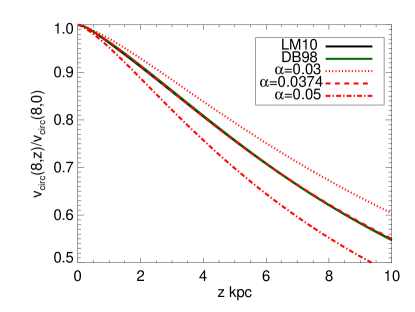
Figure 1.— Circular speed as a function of height $z$ above the mid plane for models of the Milky Way consisting of bulge, halo and disc. The non solid red lines are for the fitting formula with different values of $\alpha_{z}$. The larger the $\alpha_{z}$ the steeper is the fall of circular speed.

2.5. Models and parameters explored

We now give a description of the parameters and models that we explore. We investigate up to 18 parameters (see Table 2 for a summary). These are the Solar motion $(U_{\odot},V_{\odot},W_{\odot})$, the logarithmic slopes of age-dispersion relations $(\beta_{R},\beta_{\phi},\beta_{z})$, the scale lengths of radial dependence of velocity dispersions $(R_{\sigma}^{\rm thin},R_{\sigma}^{\rm thick})$, the velocity dispersions at $R=R_{0}$ of the thin disc $(\sigma_{\phi}^{\rm thin},\sigma_{z}^{\rm thin},\sigma_{R}^{\rm thin})$ and of the thick disc $(\sigma_{\phi}^{\rm thick},\sigma_{z}^{\rm thick},\sigma_{R}^{\rm thick})$; for simplicity the subscript $\odot$ is dropped here. The Gaussian models are denoted by GAU whereas models based on the Shu DF are denoted by SHU. For models based on the Shu DF, the azimuthal motion is coupled to the radial motion, hence $\beta_{\phi}$, $\sigma_{\phi}^{\rm thin}$ and $\sigma_{\phi}^{\rm thick}$ are not required. When $\Theta_{0}$ is fixed, we assume its value to be $226.84\,{\rm km}\,{\rm s}^{-1}$. In some cases, we also keep the parameters $\beta_{z}$ and $R_{\sigma}^{\rm thin}$ fixed. While reporting the results we highlight the fixed parameters using the magenta color.

In our analysis the distance of the Sun from the galactic center, $R_{0}$, is assumed to be 8.0 kpc. To gauge the sensitivity of our results to $R_{0}$, we also provide results for cases with $R_{0}=7.5$ and 8.5 kpc. The true value of $R_{0}$ is still debatable ranging from 6.5 to 9 kpc. Recent results from studies of orbit of stars near the Galactic Center give $R_{0}=8.33\pm 0.35$ (Gillessen et al., 2009). The classically accepted value of $8\pm 0.5$ kpc is a weighted average given in a review by Reid (1993). The main reason we keep $R_{0}$ fixed is as follows. Given that we do not make use of explicit distances, proper motions or external constraints like the proper motion of Sgr A*, it is clear we will not be able to constrain $R_{0}$ well, specially if $\Theta_{0}$ is free. For example McMillan & Binney (2010) using parallax, proper motion and line of sight velocity of masers in high star forming regions, show that constraining both $\Theta_{0}$ and $R_{0}$ independently is difficult.

3. Observational data and selection functions

In this paper we analyze data from two surveys, the Radial Velocity Experiment, RAVE (Steinmetz et al., 2006; Zwitter et al., 2008; Siebert et al., 2011; Kordopatis et al., 2013) and the Geneva Copenhagen Survey, GCS (Nordström et al., 2004; Holmberg et al., 2009). For fitting theoretical models to data from stellar surveys, it is important to take into account the selection biases that were introduced when observing the stars. This is especially important for spectroscopic surveys which observe only a subset of the all possible stars defined within a color-magnitude range. So we also analyze the selection function for the RAVE and GCS surveys.

3.1. RAVE survey

The RAVE survey collected spectra of 482430 stars between April 2004 and December 2012 and stellar parameters, radial velocity, abundance and distances have been determined for 425561 stars. In this paper we used the internal release of RAVE from May 2012, which consisted of 458412 observations. The final explored sample after applying various selection criteria consists of 280128 unique stars. These data are available in the DR4 public release (Kordopatis et al., 2013), where an extended discussion of the sample is also presented.

For RAVE we only make use of the $\ell,b$ and $v_{\rm los}$ of stars. The $I_{\rm DENIS}$ and 2MASS $J-K_{s}$ colors are used for marginalization over age, metallicity and mass of stars taking into account the photometric selection function of RAVE. We do not use proper motions, or stellar parameters which could in principle provide tighter constraints, but then one has to worry about the systematics introduced by their use. For example, in a recent kinematic analysis of RAVE stars, Williams et al. (2013) found systematic differences between different proper motion catalogs like PPMXL (Röser et al., 2008), SPM4 (Girard et al., 2011) and UCAC3 (Zacharias et al., 2010). As for stellar parameters, although they are reliable, no pipeline can claim to be free of unknown systematics specially when working with low signal to noise data. Hence, as a first step it is instructive to work with data that are least ambiguous and then in the next step check the results by adding more information. As we will show later, for the types of model that we consider, even using only $\ell,b$ and $v_{\rm los}$ can provide good constraints on the model parameters.

We now discuss the selection function of RAVE. The RAVE survey was designed to be a magnitude-limited survey in the $I$ band. This means that theoretically it has one of the simplest selection functions, but, in practice, for a multitude of reasons, some biases were introduced. First, the DENIS and 2MASS surveys were not fully available when the survey started. Hence, the first input catalog (IC1) had stars from Tycho and SuperCOSMOS. For Tycho stars, $I$ magnitudes were estimated from $V_{T}$ and $B_{T}$ magnitudes. On the other hand, the SuperCOSMOS stars had $I$ magnitudes but an offset was later detected with respect to $I_{\rm DENIS}$. Later, as DENIS and 2MASS became available, the second input catalog IC2 was created. With the availability of DENIS, it became possible to have a direct $I$ mag measurement which was free from offsets like those observed in SuperCOSMOS. But DENIS itself had its own problems – saturation at the bright end, duplicate entries, missing stripes in the sky, inter alia. To solve the problem of duplicate entries, the DENIS catalog was cross-matched with 2MASS to within a tolerance of 1^′′. This helped clean up the color-color diagram of $(I_{\rm DENIS}-K_{\rm 2MASS})$ vs $(J_{\rm 2MASS}-K_{\rm 2MASS})$ in particular (Seabroke, 2008).

Given this history, the question arises how can we compute the selection function. Since accurate $I$ mag photometry is not available for stars that are only in IC1, the first cut we make is to select stars from IC2 only. Then we removed the duplicates– among multiple observations one of them was selected randomly. To weed out stars with large errors in radial velocity, we made some additional cuts:

$${\rm Signal\ to\ Noise\ STN}>20$$

$${\rm Tonry-Davis\ Correlation\ Coefficient}>5.$$

For brighter magnitudes, $I_{\rm DENIS}<10$, $I_{\rm DENIS}$ suffers from saturation. One could either get rid of these stars to be more accurate or ignore the saturation. In the present analysis we ignore the saturation. Note, the observed stars in the input catalog are not necessarily randomly sampled from the IC2. Stars were divided into four bins in $I_{\rm mag}$ and stars in each bin were randomly selected to observe at a given time. However it seems later on this division was not strictly maintained (probably due to the observation of calibration stars and some extra stars going to brighter magnitudes). This means the selection function has to be computed as a function of $I_{\rm DENIS}$ in much finer bins. Assuming the DENIS I magnitudes are correct, and the cross-matching is correct, the only thing that needs to be taken into account is the angular completeness of the DENIS survey (missing stripes). To this end, we grid the observed and IC2 stars in $(\ell,b,I_{\rm DENIS})$ space and compute a probability map. To grid the angular co-ordinates we use the HEALPIX pixelization scheme (Górski et al., 2005). The resolution of HEALPIX is specified by the number $n_{\rm side}$ and the total number of pixels is given by $12n_{\rm side}^{2}$. For our purpose, we use $n_{\rm side}=16$ which gives a pixel size of 13.42 ${\rm deg}^{2}$, which is smaller than the RAVE field of view of 28.3 ${\rm deg}^{2}$. For magnitudes, we use a bin size of 0.1 mag, which again is much smaller than the magnitude range included in each observation. Given the fine resolution of the probability map, the angular and magnitude dependent selection biases are adequately handled. Note, in the range $(225^{\circ}<\ell<315^{\circ})\ \&\ (5^{\circ}<|b|<25^{\circ})$, a color selection of $(J-K_{s})>0.5$ was used to selectively target giants, and we take this into account in our analysis.

Arce & Goodman (1999) suggest that the Schlegel et al. (1998) maps overestimate reddening by a factor of 1.3-1.5 in regions with smooth extinction $A_{V}>0.5$, i.e., $E_{B-V}>0.15$ (see also Cambrésy et al., 2005). In LABEL:extcorr the color and temperature distributions of our RAVE stars (black lines) are compared with predictions from Galaxia given the selection above. At high latitudes (second and fourth panels) the red model curves agree reasonably well with the black data curves, but in the top panel ($5^{\circ}<|b|<25^{\circ}$) the red model distribution of $J-K$ colors is clearly displaced to red colours relative to the data. The low-latitude temperature distributions shown in the third panel show no analogous shift of the model curve to lower temperatures, so we have a clear indication that the model colours have been made too red by excessive extinction. To correct this problem, we modify the Schlegel $E_{B-V}$ as follows

$$f_{\rm corr} = 0.6+0.2\left(1-{\rm tanh}\left[\frac{E_{B-V}-0.15}{0.1}\right]\right)$$ (24)

The formula above reduces extinction by 40% for high extinction regions; the transition occurs around $E_{B-V}\sim 0.15$ and is smoothly controlled by the ${\rm tanh}$ function. The green curves in the top two panels show that the proposed correction to Schlegel maps. Although not perfect, the correction reduces the discrepancy between the model and data for low latitude stars (top panel) whilst having negligible impact on high-latitude stars.

The fact that the temperature and color distributions in LABEL:extcorr match up so well is encouraging, given that we selected on $I_{\rm DENIS}$ magnitude alone. This implies that the spatial distribution of stars specified by Galaxia satisfies one of the necessary observational constraints.

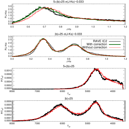
Figure 2.— The color and temperature distribution (from DR3 pipeline) of RAVE stars compared with Galaxia simulations with properly matched selection and statistical sampling. The effect of our new correction formula for the Schlegel extinction map is also shown. The results for $|b|<25^{\circ}$ and $|b|>25^{\circ}$ are shown separately. Note, Galaxia makes use of Padova isochrones.

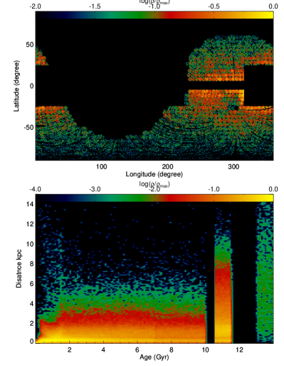
Figure 3.— Probability distribution of RAVE stars analyzed in this paper in $(\ell,b)$ space (Top) and (Age, Distance) space (Bottom). The age-distance distributions are predictions from the Galaxia model for stars satisfying the RAVE selection criteria.

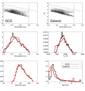
Figure 4.— Distribution of GCS stars as a function of color, temperature, distance and age. Shown alongside are results of a mock sample created using Galaxia but without observational uncertainties. The top panel shows the distribution in the $(b-y,M_{V})$ plane; the colors span the range $0.205<(b-y)<0.5$. The magnitude limits are a function of color and are taken from Nordström et al. (2004). The line represents the equation $M_{V}=10(b-y)-3$ and is used to mimic the selective avoidance of giants in GCS. A selection of $d<0.12\,{\rm kpc}$ and $T_{\rm eff}>7244$ K is also applied. The temperature and ages (maximum likelihood Padova) are from Casagrande et al. (2011).

3.2. GCS survey

We fit the models to all six phase-space coordinates of a subset of the 16682 F and G type main-sequence stars in the GCS (Nordström et al., 2004; Holmberg et al., 2009). A mock GCS sample was extracted from the model as in Sharma et al. (2011). Velocities and temperatures are available for 13382 GCS stars. We found that while Galaxia predicts less than one halo star in the GCS sample for a distance less than $120$ pc, when plotted in $({\rm[Fe/H]},v_{\phi})$ plane, the GCS has 29 stars with ${\rm[Fe/H]}<-1.2$ and highly negative values of $v_{\phi}$ (as expected for halo stars). Following Schönrich et al. (2010), we identify these as halo stars and exclude them from our analysis.

The GCS catalog is complete for F and G type stars within a volume given by $r<40$ pc and $V\sim 8$ in magnitude; within these limits there are only 1342 stars. But since GCS is a color-magnitude limited survey, there is no need to restrict the analysis to a volume complete sample. In Nordström et al. (2004) magnitude completeness as a function of color is provided and we use this (their §2.2). There is some ambiguity about the coolest dwarfs which were added for declination $\delta<-26^{\circ}$; from information gleaned from Nordström et al. (2004), we could not find a suitable way to take this into account.

We also applied some additional restrictions on the sample. For example, we restrict our analysis to stars with distance less than 120 pc, so as to avoid stars with large distance errors. The GCS survey selectively avoids giants. To mimic this we use the following selection function $M_{V}<10(b-y)-3$. The predicted temperature distributions show a mismatch with models, in particular, there are too many hot stars. Using Casagrande et al. (2011) temperatures, which are more accurate, we found an upper limit on $T_{\rm eff}$ of 7244 K, which was applied to the models.

After the above mentioned cuts, the final sample consisted of 5201 stars. Note, we do not remove possible binary stars as this will further reduce the number of stars. In future, we think it will be instructive to check if there is any systematic associated with the inclusion or exclusion of binaries. The black histograms in LABEL:gcs2 show the distribution of these stars, while the red histograms show the predictions of the model. At the hot end, the temperature distributions of model and data are still discrepant, but the distance distributions agree nicely. The model’s age distribution is qualitatively correct but differences can also be seen. The plotted GCS ages are maximum likelihood Padova ages and there can be systematics associated with this. A more quantitative comparison would require estimating the ages of model stars in the same way as done by GCS and taking into account uncertainties and systematics which we do not do here. The peak in the model at 11 Gyr is due to the thick disc having a fixed age. The peaks in the data at 0 and $14\,{\rm Gyr}$ are most likely due to caps employed while estimating ages. The color distribution in GCS shows a peak at around $b-y=0.3$, which could be due to an unknown selection effect. The bump at $b-y\sim 0.43$, which is also seen in models, is due to turnoff stars. Overall, we think our modelling reproduces to a good degree the selection function of the GCS stars.

4. Model Fitting techniques

If $y_{i}$ are the observed properties of a star, we can describe the observed data by $y=\left\{y_{i}\in\mathbb{R}^{d},0<i<N\right\}$. Also, let $\theta$ be the set of parameters that define the model. Our job is to compute

$$p(\theta|y)\propto p(y|\theta)p(\theta)$$ (25)

where $p(y|\theta)=\prod_{i}p(y_{i}|\theta)$. We employ an MCMC scheme to estimate $p(\theta|y)$ and assume a uniform prior on $\theta$. We now discuss how to compute $p(y_{i}|\theta)$.

Generally, a model of a galaxy gives the probability density $p({\bf r,v},\tau,Z,m|\theta)$. For RAVE, the observed quantities are $v_{\rm los},l$ and $b$, while for GCS they are $l,b,r,v_{l},v_{b}$ and $v_{\rm los}$. Since quantities like $\tau,Z$ and $m$ are unknown, one has to compute the marginal probability density by integration. For RAVE, the required marginal density is

$$p(\ell,b,v_{\rm los}|\theta) = \int p(\ell,b,r,\tau,Z,m,v_{l},v_{b},v_{\rm los}|\theta)$$ (26)

$$\times S(\ell,b,\tau,Z,m)\>dr\>d\tau\>dZ\>dm\>dv_{l}\>dv_{b},$$

and for GCS it is

$$p(\ell,b,r,v_{l},v_{b},v_{\rm los}|\theta) = \int p(\ell,b,r,\tau,Z,m,v_{l},v_{b},v_{\rm los}|\theta)$$ (27)

$$\times S(\ell,b,\tau,Z,m)\>d\tau\>dZ\>dm.$$

Here $S(\ell,b,\tau,Z,m)$ is the selection function specifying how the stars were preselected in the data. The actual selection is on photometric magnitude which in turn is a function of $\tau,Z$ and $m$.

For the kinds of models explored here, the computations are considerably simplified due to the fact that

$$p(\ell,b,r,\tau,Z,m,v_{l},v_{b},v_{\rm los}|\theta) = p(v_{l},v_{b},v_{\rm los}|\ell,b,r,\tau,\theta)$$

$$\times p(\ell,b,r,\tau,Z,m|\theta_{S}),$$ (28)

for which $\theta_{S}$ is the set of model parameters that govern the spatial distribution of stars and $\theta$ is the set of model parameters that govern the kinematic distribution of stars. The term $p(\ell,b,r,\tau,Z,m|\theta_{S})$ is invariant in our analysis, and this is the main assumption that we make. In other words we assume star formation rate (SFR), initial mass function (IMF), scale length of disc, age scale-height relation, age metallicity relation and radial metallicity gradient for the disc. All these distributions can be constrained by the stellar photometry. The distribution $p(v_{l},v_{b},v_{\rm los}|\ell,b,r,\tau,\theta)$ represents the kinematics, which is what we explore. It should be noted that the model $p(\ell,b,r,\tau,Z,m|\theta_{S})$ that we use has been shown to satisfy the number count of stars (Robin et al., 2003; Sharma et al., 2011). In a fully self consistent model, the scale height, the vertical stellar velocity dispersion and the potential would all be related to each other and this is something we would like to address in future.

We can now integrate the last term in Equation (28) over $m$ and $Z$ such that

$$p(\ell,b,r,v_{l},v_{b},v_{\rm los},\tau|\theta) = p(v_{l},v_{b},v_{\rm los}|\ell,b,r,\tau,\theta)$$ (29)

$$\times p(\ell,b,r,\tau|\theta_{S},S)$$

where

$$p(\ell,b,r,\tau|\theta_{S},S) = \int\int p(\ell,b,r,\tau,Z,m|\theta_{S})$$ (30)

$$\times S(\ell,b,\tau,Z,m)\>dZ\>dm.$$

The term $p(\ell,b,r,\tau|\theta_{S},S)$ is computed numerically using the code Galaxia (Sharma et al., 2011). Galaxia, uses isochrones from the Padova database to compute photometric magnitudes for the model stars (Marigo et al., 2008; Bertelli et al., 1994). We first generate a fiducial set of stars satisfying the color-magnitude range of the survey. Then we apply the selection function and reject stars that do not satisfy the constraints of the survey. The accepted stars are then binned in $(\ell,b,r,\tau)$ space. Since, the GCS is local to the Sun, we use the following approximation $p(\ell,b,r,\tau|\theta_{S},S)\propto p(\tau|\theta_{S},S)$. The probability distribution in $(\ell,b,r,\tau)$ space for RAVE is shown in LABEL:rave_stat1.

For RAVE, we have to integrate over four variables ($r,\tau,v_{l},v_{b}$), but for GCS we integrate over only $\tau$. The 4D marginalization for RAVE poses a serious computational challenge for data as large as the RAVE survey. For Gaussian distribution functions, the integral over $v_{l}$ and $v_{b}$ can be performed analytically to give an analytic expression for $p(v_{\rm los}|\ell,b,r,\tau,Z,\theta)$, but in general it cannot be done analytically. Hence, we try two new methods. The first method is fast but has inflated uncertainties. The second method is slower to converge but gives correct estimates of uncertainties. Given these strengths and limitations, we use a combined strategy that makes best use of both the methods.

We use the first ‘sampling and projection’ method to get an initial estimate of $\theta$ and also its covariance matrix. These are then used in the second ‘data augmentation’ method. The initial estimate reduces the ‘burn in’ time, while the covariance matrix eliminates the need to tune the widths of the proposal distributions. In general we use an adaptive MCMC scheme, which avoids manual tuning of the widths of the proposal distributions (Andrieu & Thoms, 2008). At regular intervals, we compute the covariance matrix and scale it so as to achieve the desired acceptance ratio for the given number of parameters Gelman et al. (1996). We now discuss the two methods in more detail.

4.1. MCMC using sampling and projection

Instead of doing the computationally intensive marginalization, at each step of the Markov chain of model parameters, we generate a sample of stars by Monte-Carlo sampling the current model subject to the selection function. Binning these stars in $(\ell,b,v_{\rm los})$ space then gives an estimate of $p(\ell,b,v_{\rm los}|\theta)$. Note that, given the stochastic nature of our estimate of $p(\ell,b,v_{\rm los}|\theta)$, the standard Metropolis-Hastings algorithm had to be altered to avoid the simulation from getting stuck at a stochastic maximum of the likelihood.

4.2. MCMC using data augmentation

Instead of marginalizing one can treat the nuisance parameters as unknown parameters and estimate them alongside other parameters. This constitutes what is known as a sampling based approach for computing the marginal densities. The basic form of this scheme was introduced by Tanner & Wong (1987) and later extended by Gelfand & Smith (1990). Let $x=\left\{x_{i}\in\mathbb{R}^{d},0<i<N\right\}$ be an extra set of variables that are needed by the model to compute the probability density. Then we can write

$$p(\theta,x|y)\propto p(x,y|\theta)p(\theta).$$ (31)

where $p(x,y|\theta)=\prod_{i}p(x_{i},y_{i}|\theta)$, and $p(x_{i},y_{i}|\theta)$ is a function which is known and relatively easy to compute. For example, for the RAVE data $y_{i}=\left\{l_{i},b_{i},v_{i,{\rm los}}\right\}$ and $x=\left\{r_{i},\tau_{i},v_{l,i},v_{b,i}\right\}$. Due to the unusually large number of parameters, it is difficult to get satisfactory acceptance rates with the standard Metropolis-Hastings scheme without making the widths of the proposal distributions extremely small. Thus the chains would take an unusually long time to mix. To solve this, one uses the Metropolis scheme with Gibbs sampling (MWG) (Tierney, 1994). The MWG scheme is also useful for solving hierarchical Bayesian models, and its application for 3D extinction mapping is discussed in Sale (2012). In our case, the Gibbs step consists of first sampling $x$ from the conditional density $p(x|y,\theta)$ and then $\theta$ from the conditional density $p(\theta|y,x)$. The sampling in each Gibbs step is done using the Metropolis-Hastings algorithm.

4.3. Goodness of fit

To assess the ability of a model to fit the data, we compute an approximate reduced $\chi^{2}$ value. To accomplish this, first we bin the data in the observational space. For RAVE, we bin the data in $(l,b,v_{\rm los})$ space with bins of size 859 deg² and $5\,{\rm km}\,{\rm s}^{-1}$. Angular binning was done using the HEALPIX scheme. For GCS, we bin the $U,V$ and $W$ components of velocity separately with bins of size $5\,{\rm km}\,{\rm s}^{-1}$. Next, an N-body realization of a given model was created satisfying the same constraints as the data, The reduced $\chi^{2}$ between the data and the model was then computed as

$$\chi_{\rm red}^{2}=\Bigl{\langle}\sum_{i}\frac{(n_{i}-m_{i}/f_{\rm sample})^{2}}{n_{i}+m_{i}/f_{\rm sample}^{2}}\Bigr{\rangle}{\ \rm for\ }n_{i}>0.$$ (32)

Here, $n_{i}$ is the number of data points in a bin, $m_{i}$ the number of model points in the same bin and $f_{\rm sample}=\sum_{i}m_{i}/\sum_{i}n_{i}$ is the sampling fraction. Choosing, $f_{\rm sample}$ to be very high one can increase the precision of the estimate, but then it increases the computational cost. For RAVE $f_{\rm sample}$ was 1 while for GCS it was 10. To decrease the stochasticity in the estimate, we computed the mean over 30 random estimates $\langle\chi_{\rm red}^{2}\rangle=\sum_{k=1}^{30}\chi_{\rm red,k}^{2}/30$.

The reduced $\chi^{2}$ as computed above, has its limitations. Firstly, it is not an accurate estimator of the goodness of fit. Secondly, $\chi^{2}$ value is sensitive to the choice of bin size and $f_{\rm sample}$. Hence, it is not advisable to estimate statistical significance using our reduced $\chi^{2}$. However, the reduced $\chi^{2}$ should be good enough to qualitatively compare the goodness of fit of two models.

4.4. Tests using synthetic data

We now describe tests in which mock data are sampled from the distribution function and then fitted using the MCMC machinery. These tests serve two main purposes. First, they determine if our MCMC scheme works correctly. Secondly, they tell us which parameters can be recovered and with what accuracy. We study two classes of models based on (1) the Gaussian DF and (2) the Shu DF. Additionally, we study two types of mock data, one corresponding to the RAVE survey and the other to the GCS survey. For GCS we also study models where $\Theta_{0}$ is fixed. Altogether this leads to 6 different types of tests.

The results of these tests are summarized in Tables 4 and 4. The difference of a parameter $p$ from input values divided by uncertainty $\sigma_{p}$ measures the confidence of recovering the parameter. To aid the comparison, we color the values if they differ significantly from the input values: $|\delta p|/\sigma_{p}<2$ (black), $2<|\delta p|/\sigma_{p}<3$ (blue). It can be seen that all parameters are recovered within the 3$\sigma$ range as given by the error bars. Ideally to check the systematics, the fitting should be repeated multiple times and the mean values should be compared with input values. However, the MCMC simulations being computationally very expensive we report results with only one independent data sample for each of the test cases.

It can be seen that GCS type data cannot properly constrain $\Theta_{0}$. This is because the GCS sample is very local to the Sun. Keeping $\Theta_{0}$ free also has the undesirable effect of increasing the uncertainty of $R_{\sigma}^{\rm thin}$ and $R_{\sigma}^{\rm thick}$. For Gaussian models, it is easy to see from Equation (6) that the effect of changing $\Theta_{0}$ can be compensated by a change in $R_{\sigma}^{\rm thin}$ and $R_{\sigma}^{\rm thick}$. Given these limitations, when analyzing GCS we keep $\Theta_{0}$ fixed to 226.87 km s^-1, a value that was used by Sharma et al. (2011) in the Galaxia code.

The Solar motion is constrained well by both surveys, but better by RAVE. RAVE is also clearly better in constraining thick-disc parameters than GCS, mainly because the GCS has very few thick-disc stars (Galaxia estimates it to be 6% of the overall GCS sample). Across all parameters, for Shu models $\beta_{z}$ is the only parameter which is constrained better by GCS than by RAVE. This is because RAVE only has radial velocities. This means that only those stars that lie towards the pole can carry meaningful information about the vertical motion, and such stars constitute a much smaller subset of the whole RAVE sample. This suggests that one can use the $\beta_{z}$ value from GCS when fitting the RAVE data, as we show below.

Table 3 Tests on mock data: Constraints on model parameters with Gaussian distribution function. The model runs are named as follows; survey name as RAVE or GCS, type of model as GAU for Gaussian and SHU for Shu. Parameters that do not have error bars were fixed. Velocities are in $\,{\rm km}\,{\rm s}^{-1}$ and distances in ${\rm kpc}$

Model	GCS GAU	GCS GAU	RAVE GAU	Input
$U_{\odot}$	$11.12_{-0.41}^{+0.43}$	$11.17_{-0.39}^{+0.39}$	$11.22_{-0.16}^{+0.15}$	$11.1$
$V_{\odot}$	$5.8_{-1.9}^{+1.8}$	$8.6_{-1.3}^{+1.3}$	$8.16_{-0.24}^{+0.29}$	$7.5$
$W_{\odot}$	$7.14_{-0.19}^{+0.19}$	$7.35_{-0.18}^{+0.19}$	$7.377_{-0.087}^{+0.092}$	$7.25$
$\sigma_{R}^{\rm thin}$	$38.5_{-1.6}^{+1.7}$	$42.7_{-1.6}^{+1.6}$	$40.45_{-0.84}^{+0.56}$	$40$
$\sigma_{\phi}^{\rm thin}$	$28.8_{-1}^{+1.1}$	$28.4_{-1.1}^{+1.1}$	$27.7_{-0.5}^{+0.42}$	$28.3$
$\sigma_{z}^{\rm thin}$	$25.03_{-0.84}^{+0.86}$	$25.89_{-0.86}^{+0.87}$	$25.09_{-0.72}^{+0.6}$	$25$
$\sigma_{R}^{\rm thick}$	$63.3_{-3.8}^{+3.8}$	$55.3_{-4}^{+4.2}$	$60.62_{-0.68}^{+0.55}$	$60$
$\sigma_{\phi}^{\rm thick}$	$47.8_{-2.9}^{+3.1}$	$43.7_{-3.1}^{+3.2}$	$42.02_{-0.4}^{+0.45}$	$42.4$
$\sigma_{z}^{\rm thick}$	$34.1_{-2.1}^{+2.3}$	$32.8_{-2.3}^{+2.3}$	$35.19_{-0.52}^{+0.58}$	$35$
$\beta_{R}$	$0.183_{-0.025}^{+0.025}$	$0.249_{-0.023}^{+0.021}$	$0.2079_{-0.015}^{+0.0094}$	$0.2$
$\beta_{\phi}$	$0.216_{-0.022}^{+0.023}$	$0.197_{-0.023}^{+0.022}$	$0.177_{-0.016}^{+0.013}$	$0.2$
$\beta_{z}$	$0.38_{-0.022}^{+0.022}$	$0.401_{-0.022}^{+0.02}$	$0.368_{-0.03}^{+0.025}$	$0.37$
$1/R_{\sigma}^{\rm thin}$	$0.145_{-0.064}^{+0.067}$	$0.055_{-0.061}^{+0.077}$	$0.072_{-0.0058}^{+0.005}$	$0.072$
$1/R_{\sigma}^{\rm thick}$	$0.107_{-0.034}^{+0.04}$	$0.133_{-0.074}^{+0.065}$	$0.1341_{-0.0029}^{+0.0029}$	$0.132$
$\Theta_{0}$	$233$	$265_{-60}^{+63}$	$236_{-1.4}^{+1.7}$	$233$
$R_{0}$	$8$	$8$	$8$	$8$
$\alpha_{z}$	$0.047$	$0.047$	$0.0432_{-0.0019}^{+0.0015}$	$0.047$
$\alpha_{R}$	$0$	$0$	$0$	$0$
$\chi_{\rm red}^{2}$	1.09	1.00	0.935

Table 4 Tests on mock data: Constraints on model parameters with Shu distribution function

Model	GCS SHU	GCS SHU	RAVE SHU	Input
$U_{\odot}$	$11.28_{-0.41}^{+0.42}$	$11.16_{-0.41}^{+0.42}$	$11.27_{-0.14}^{+0.12}$	$11.1$
$V_{\odot}$	$7.14_{-0.36}^{+0.34}$	$7.35_{-0.67}^{+0.79}$	$7.94_{-0.15}^{+0.17}$	$7.5$
$W_{\odot}$	$6.95_{-0.2}^{+0.19}$	$6.99_{-0.2}^{+0.2}$	$7.26_{-0.088}^{+0.079}$	$7.25$
$\sigma_{R}^{\rm thin}$	$41_{-1.1}^{+1.1}$	$40.7_{-1.2}^{+1.1}$	$41.19_{-0.6}^{+0.47}$	$40$
$\sigma_{z}^{\rm thin}$	$25.18_{-0.84}^{+0.84}$	$24.9_{-0.92}^{+0.95}$	$24.62_{-0.65}^{+0.81}$	$25$
$\sigma_{R}^{\rm thick}$	$45.2_{-3.5}^{+3.6}$	$44.3_{-4}^{+3.9}$	$46.1_{-0.58}^{+0.61}$	$45$
$\sigma_{z}^{\rm thick}$	$36.8_{-2.4}^{+2.6}$	$32.3_{-2.5}^{+2.4}$	$34.3_{-0.51}^{+0.52}$	$35$
$\beta_{R}$	$0.203_{-0.016}^{+0.016}$	$0.201_{-0.017}^{+0.017}$	$0.211_{-0.013}^{+0.01}$	$0.2$
$\beta_{z}$	$0.379_{-0.021}^{+0.021}$	$0.371_{-0.024}^{+0.023}$	$0.331_{-0.025}^{+0.036}$	$0.37$
$1/R_{\sigma}^{\rm thin}$	$0.0696_{-0.0075}^{+0.0071}$	$0.074_{-0.011}^{+0.015}$	$0.0682_{-0.0026}^{+0.0027}$	$0.072$
$1/R_{\sigma}^{\rm thick}$	$0.133_{-0.016}^{+0.016}$	$0.131_{-0.017}^{+0.018}$	$0.1307_{-0.0027}^{+0.0025}$	$0.132$
$\Theta_{0}$	$233$	$224_{-20}^{+33}$	$235.1_{-1.3}^{+1.3}$	$233$
$R_{0}$	$8$	$8$	$8$	$8$
$\alpha_{z}$	$0.047$	$0.047$	$0.0427_{-0.0018}^{+0.0019}$	$0.047$
$\alpha_{R}$	$0$	$0$	$0$	$0$
$\chi_{\rm red}^{2}$	0.960	0.996	0.928

Table 5 Fiducial model parameters: Velocities are in $\,{\rm km}\,{\rm s}^{-1}$ and distances in ${\rm kpc}$

Model	Galaxia	Equivalent Besançon
$U_{\odot}$	$11.1$	$10.3$
$V_{\odot}$	$12.24$	$6.3$
$W_{\odot}$	$7.25$	$5.9$
$\sigma_{R}^{\rm thin}$	$50$	$50$
$\sigma_{\phi}^{\rm thin}$	$32.3$	$32.3$
$\sigma_{z}^{\rm thin}$	$21$	$21$
$\sigma_{R}^{\rm thick}$	$67$	$67$
$\sigma_{\phi}^{\rm thick}$	$51$	$51$
$\sigma_{z}^{\rm thick}$	$42$	$42$
$\beta_{R}$	$0.33$	$0.33$
$\beta_{\phi}$	$0.33$	$0.33$
$\beta_{z}$	$0.33$	$0.33$
$\tau_{\rm sat}$	6.5 Gyr	6.5 Gyr
$1/R_{\sigma}^{\rm thin}$	$0.133$	$0.096(0.114)$
$1/R_{\sigma}^{\rm thick}$	$0.133$	$0.176(0.2)$
$R_{0}$	$8.0$	$8.5(8.0)$
$\Theta_{0}$	$226.84$	$220.0$
$R_{d}$	$2.5$	$2.5$

Table 6 Constraints on model parameters with the Gaussian distribution function. Parameters that do not have error bars were fixed. Missing values imply parameters that are not applicable for that model. The model runs are named as follows; survey name as RAVE or GCS, type of model as GAU for Gaussian and SHU for Shu. Velocities are in $\,{\rm km}\,{\rm s}^{-1}$ and distances in ${\rm kpc}$. Quoted uncertainties are purely random and do not include systematics.

Model	GCS GAU	GCS GAU	GCS GAU	RAVE GAU	RAVE GAU	RAVE GAU
$U_{\odot}$	$10.16_{-0.42}^{+0.41}$	$10.28_{-0.43}^{+0.43}$	$10.34_{-0.42}^{+0.42}$	$11.66_{-0.15}^{+0.16}$	$11.45_{-0.14}^{+0.14}$	$11.25_{-0.15}^{+0.15}$
$V_{\odot}$	$6.6_{-1.4}^{+1.3}$	$6.33_{-0.97}^{+0.93}$	$9.68_{-0.26}^{+0.26}$	$15.01_{-0.42}^{+0.37}$	$8_{-0.28}^{+0.3}$	$7.38_{-0.12}^{+0.1}$
$W_{\odot}$	$7.14_{-0.18}^{+0.19}$	$7.11_{-0.19}^{+0.19}$	$7.14_{-0.18}^{+0.18}$	$7.692_{-0.082}^{+0.099}$	$7.688_{-0.091}^{+0.085}$	$7.625_{-0.082}^{+0.088}$
$\sigma_{R}^{\rm thin}$	$41.2_{-1.3}^{+1.4}$	$47_{-1.1}^{+1.1}$	$41.5_{-1.3}^{+1.4}$	$36.6_{-1.1}^{+1}$	$39.26_{-0.69}^{+0.67}$	$39.69_{-0.65}^{+0.62}$
$\sigma_{\phi}^{\rm thin}$	$27.12_{-0.86}^{+0.89}$	$31.61_{-0.79}^{+0.8}$	$27.83_{-0.88}^{+0.88}$	$24.97_{-0.36}^{+0.43}$	$25.56_{-0.37}^{+0.33}$	$25.34_{-0.33}^{+0.35}$
$\sigma_{z}^{\rm thin}$	$23.74_{-0.74}^{+0.79}$	$27.28_{-0.63}^{+0.64}$	$23.89_{-0.74}^{+0.79}$	$24.22_{-0.47}^{+0.64}$	$25.69_{-0.2}^{+0.22}$	$25.92_{-0.2}^{+0.21}$
$\sigma_{R}^{\rm thick}$	$65.9_{-3.7}^{+4.1}$		$67.7_{-2.7}^{+2.7}$	$58.74_{-0.79}^{+0.91}$	$58.43_{-0.76}^{+0.86}$	$57.87_{-0.56}^{+0.58}$
$\sigma_{\phi}^{\rm thick}$	$40.9_{-3.1}^{+3.3}$		$40_{-2.8}^{+2.9}$	$40.47_{-0.48}^{+0.51}$	$37.16_{-0.53}^{+0.5}$	$38.37_{-0.54}^{+0.48}$
$\sigma_{z}^{\rm thick}$	$38.5_{-2.5}^{+2.8}$		$38.7_{-2.6}^{+2.7}$	$40.55_{-0.49}^{+0.46}$	$40.4_{-0.5}^{+0.5}$	$39.41_{-0.48}^{+0.48}$
$\beta_{R}$	$0.201_{-0.019}^{+0.019}$	$0.268_{-0.014}^{+0.015}$	$0.204_{-0.019}^{+0.019}$	$0.06_{-0.029}^{+0.023}$	$0.135_{-0.015}^{+0.015}$	$0.164_{-0.013}^{+0.012}$
$\beta_{\phi}$	$0.271_{-0.019}^{+0.019}$	$0.349_{-0.015}^{+0.016}$	$0.284_{-0.019}^{+0.019}$	$0.132_{-0.013}^{+0.014}$	$0.17_{-0.012}^{+0.012}$	$0.164_{-0.012}^{+0.012}$
$\beta_{z}$	$0.36_{-0.021}^{+0.02}$	$0.432_{-0.016}^{+0.015}$	$0.365_{-0.02}^{+0.02}$	$0.312_{-0.02}^{+0.026}$	$0.37$	$0.37$
$1/R_{\sigma}^{\rm thin}$	$0.171_{-0.043}^{+0.046}$	$0.179_{-0.027}^{+0.028}$	$0.073$	$-0.0556_{-0.0077}^{+0.0078}$	$0.0188_{-0.0053}^{+0.0055}$	$0.073$
$1/R_{\sigma}^{\rm thick}$	$0.148_{-0.035}^{+0.04}$		$0.132$	$0.1123_{-0.0043}^{+0.0044}$	$0.0907_{-0.0036}^{+0.0035}$	$0.132$
$\Theta_{0}$	$226.84$	$226.84$	$233$	$207.2_{-1.9}^{+1.9}$	$229.2_{-2}^{+1.8}$	$234.1_{-1.4}^{+1.4}$
$R_{0}$	$8$	$8$	$8$	$8$	$8$	$8$
$\alpha_{z}$	$0$	$0$	$0.047$	$0$	$0.0738_{-0.0023}^{+0.0021}$	$0.047$
$\alpha_{R}$	$0$	$0$	$0$	$0$	$0$	$0$
$\chi_{\rm red}^{2}$ RAVE	2.55	3.19	2.49	1.89	1.64	1.79
$\chi_{\rm red}^{2}$ GCS	3.09	3.48	3.15	6.60	5.81	5.10

Table 7 Constraints on model parameters with the Shu distribution function. See Table 7 for further description.

Model	GCS SHU	GCS SHU	GCS SHU	RAVE SHU	RAVE SHU	RAVE SHU	RAVE SHU
$U_{\odot}$	$10.02_{-0.4}^{+0.39}$	$10.16_{-0.4}^{+0.39}$	$10.23_{-0.4}^{+0.39}$	$11.2_{-0.13}^{+0.13}$	$10.92_{-0.14}^{+0.13}$	$10.96_{-0.13}^{+0.14}$	$11.05_{-0.16}^{+0.15}$
$V_{\odot}$	$9.95_{-0.3}^{+0.3}$	$9.81_{-0.28}^{+0.28}$	$9.83_{-0.29}^{+0.3}$	$9.71_{-0.11}^{+0.12}$	$7.53_{-0.16}^{+0.16}$	$7.53_{-0.16}^{+0.16}$	$7.62_{-0.16}^{+0.13}$
$W_{\odot}$	$7.14_{-0.19}^{+0.19}$	$7.13_{-0.19}^{+0.18}$	$7.12_{-0.19}^{+0.18}$	$7.536_{-0.086}^{+0.085}$	$7.542_{-0.093}^{+0.089}$	$7.539_{-0.09}^{+0.095}$	$7.553_{-0.09}^{+0.086}$
$\sigma_{R}^{\rm thin}$	$38.14_{-0.94}^{+0.98}$	$39.99_{-0.91}^{+0.91}$	$42.71_{-0.8}^{+0.83}$	$42.37_{-0.66}^{+0.61}$	$39.78_{-0.73}^{+0.81}$	$39.67_{-0.72}^{+0.63}$	$39.56_{-0.7}^{+0.66}$
$\sigma_{z}^{\rm thin}$	$23.39_{-0.73}^{+0.77}$	$23.63_{-0.8}^{+0.85}$	$25.91_{-0.6}^{+0.64}$	$26.85_{-0.92}^{+0.85}$	$24.7_{-0.66}^{+0.66}$	$25.73_{-0.21}^{+0.21}$	$25.72_{-0.25}^{+0.23}$
$\sigma_{R}^{\rm thick}$	$70.1_{-5.5}^{+3.7}$	$45.9_{-1.8}^{+1.8}$		$38.84_{-0.96}^{+1.2}$	$42.31_{-0.9}^{+1}$	$42.43_{-1}^{+0.95}$	$43.23_{-1.1}^{+0.96}$
$\sigma_{z}^{\rm thick}$	$39_{-3.3}^{+3.1}$	$32.6_{-2.2}^{+2.3}$		$29.15_{-0.79}^{+0.87}$	$34.66_{-0.58}^{+0.61}$	$34.3_{-0.57}^{+0.51}$	$34.48_{-0.53}^{+0.54}$
$\beta_{R}$	$0.213_{-0.014}^{+0.014}$	$0.237_{-0.013}^{+0.013}$	$0.273_{-0.011}^{+0.011}$	$0.236_{-0.011}^{+0.011}$	$0.198_{-0.014}^{+0.014}$	$0.195_{-0.013}^{+0.011}$	$0.192_{-0.013}^{+0.012}$
$\beta_{z}$	$0.361_{-0.02}^{+0.02}$	$0.366_{-0.021}^{+0.021}$	$0.415_{-0.016}^{+0.016}$	$0.398_{-0.029}^{+0.03}$	$0.328_{-0.024}^{+0.027}$	$0.37$	$0.37$
$1/R_{\sigma}^{\rm thin}$	$0.0665_{-0.0086}^{+0.0084}$	$0.073$	$0.0771_{-0.0061}^{+0.0059}$	$0.0673_{-0.0028}^{+0.0028}$	$0.0722_{-0.0032}^{+0.0035}$	$0.073_{-0.003}^{+0.0037}$	$0.0724_{-0.0031}^{+0.0031}$
$1/R_{\sigma}^{\rm thick}$	$0.0086_{-0.0066}^{+0.022}$	$0.132$		$0.1555_{-0.0064}^{+0.0046}$	$0.1335_{-0.0056}^{+0.0046}$	$0.1328_{-0.0051}^{+0.005}$	$0.13_{-0.0046}^{+0.0056}$
$\Theta_{0}$	$226.84$	$232$	$226.84$	$212.6_{-1.3}^{+1.4}$	$232.8_{-1.6}^{+1.7}$	$231.9_{-1.5}^{+1.4}$	$235.02_{-0.83}^{+0.86}$
$R_{0}$	$8$	$8$	$8$	$8$	$8$	$8$	$8$
$\alpha_{z}$	$0$	$0.0471$	$0$	$0$	$0.048_{-0.0018}^{+0.0019}$	$0.0471_{-0.0019}^{+0.0016}$	$0.0471_{-0.0019}^{+0.0019}$
$\alpha_{R}$	$0$	$0$	$0$	$0$	$0$	$0$	$0.67_{-0.26}^{+0.25}$
$\chi_{\rm red}^{2}$ RAVE	2.07	1.80	2.40	1.52	1.43	1.42	1.42
$\chi_{\rm red}^{2}$ GCS	3.85	3.86	4.08	5.15	5.57	5.42	5.46

5. Constraints on kinematic parameters

First, we discuss the fiducial parametric model for the Galaxy developed a decade ago by Robin et al. (2003). The so-called Besançcon model is based on Gaussian velocity ellipsoid functions. In the Galaxia code, the tabulated functions of Robin et al. (2003) were replaced by analytic expressions, the parameters of which are given in Table 5. One main difference between the Galaxia and Besançon models is the value of $R_{0}$ and the Solar motion with respect to the LSR. Also, Galaxia uses slightly different values of $R_{\sigma}$. In the Besançon model, the velocity dispersions are assumed to saturate abruptly at around $\tau_{\rm sat}=6.5$ Gyr. Moreover, the velocity dispersion of the thick disc does not have any radial dependence, hence the value of $R_{\sigma}^{\rm thick}$ only contributes to the calculation of the asymmetric drift. Neither of these Ansätze are assumed in our analysis.

Finally, in the Besançon model, the metallicity [Fe/H] of the thick disc is assumed to be $-0.78$ with a spread of 0.3 dex. The spread is not taken into account when assigning magnitudes and colors from isochrones. This was done so as to prevent the thick disc from having a horizontal branch. We do not make this ad hoc assumption. Since our data do not have a strong color-sensitive selection, this has a negligible impact on our kinematic study.

We now discuss the results obtained from fitting models to the RAVE and the GCS data. The best-fit parameters and their uncertainties obtained using MCMC simulation for different models and data are shown in Table 7 and Table 7. Note, the uncertainties quoted in the table are purely random and do not include systematics. We discuss systematics separately in Section 6.8. We begin by discussing results from the Gaussian distribution function before proceeding to the Shu distribution function.

5.1. Gaussian models

First we concentrate on GCS data (column 1 of Table 7). For GCS we find that all the values are well constrained. However, percentage wise $R_{\sigma}^{\rm thin},R_{\sigma}^{\rm thick}$ and $V_{\odot}$ have larger uncertainties as compared to other parameters. In LABEL:gcs_UVW3, where fits from column 1 are plotted, it can be seen that the model is an acceptable fit to the data. The reduced $\chi^{2}$ values are quite high especially in comparison to the mock models. This is mainly due to significant amount of structure in $(U,V)$ velocity space (see LABEL:gcs_UVW3). The $\beta_{z}$, $\sigma_{z}^{\rm thin}$, $\sigma_{z}^{\rm thick}$ and $\sigma_{R}^{\rm thick}$ parameters are close to the corresponding Besançon values but show other differences. The most notable differences are that our value for $R_{\sigma}^{\rm thin}$ is smaller, $R_{\sigma}^{\rm thick}$ is longer, and $\sigma_{\phi}^{\rm thick}$ is lower. Other minor differences are as follows. Our $\beta_{R}$ and $\beta_{\phi}$ are lower and so are the velocity dispersions $\sigma_{R}^{\rm thin}$, $\sigma_{\phi}^{\rm thin}$. The thin-disc velocity dispersions are strongly correlated to $\beta$ values, so fixing $\beta$ to higher values will drive the corresponding thin-disc velocity dispersions closer to the Besançon values. The second column in Table 7 shows the results for the case where a separate thick disc is not assumed (the thick-disc stars are labelled as thin-disc in the model). In this case, $\beta$, $\sigma$ increase, while $R_{\sigma}^{\rm thin}$ decreases, which is expected since the thin disc has to accommodate the warmer thick disc component.

We now discuss results for the RAVE data, beginning with the model where $\alpha_{z}=0$ (column 4 of Table 7). Surprisingly, $R_{\sigma}^{\rm thin}$ is found to be negative, whereas the $R_{\sigma}^{\rm thick}$ is positive. The value of $\Theta_{0}$ is found to be significantly less than that reported in literature. The $\beta_{R}$ and $\beta_{\phi}$ values are also too small. We note that the $\beta_{z}$ value in RAVE has more uncertainty than that in GCS, which we had also noted in the tests on mock data. From now on we keep $\beta_{z}=0.37$, a value we get from GCS. We checked and found that fixing $\beta_{z}$ has negligible impact on other parameters.

We now let $\alpha_{z}$ free and this results in higher value of $\Theta_{0}$. The value of $\Omega_{\odot}$ is now close to the proper motion of Sgr A*. Allowing for a vertical dependence of circular speed decreases $R_{\sigma}^{\rm thin}$ while increasing $\beta_{R}$ and $\beta_{\phi}$. However, these values are still lower than the GCS values. It can be seen from red lines in LABEL:rave_UVW1 that the model does not fit well the projected $V$ components of velocity. Clearly there are some problems with this model.

We now compare RAVE and GCS results using columns 6 and 3, where we fix $R_{\sigma}^{\rm thin}$, $R_{\sigma}^{\rm thick}$ and $\alpha_{z}$ to values that we will get later from the Shu model. Having the same value of $R_{\sigma}$ in both RAVE and GCS makes it easier to compare the other parameters. Naturally, fixing some of the variables leads to an increased $\chi_{\rm red}^{2}$. We find that most of the values agree to within 4$\sigma$ of each other. The two exceptions are $\beta_{\phi}$ and $V_{\odot}$ which are higher for GCS.

To summarize, we find that the model parameters that best fit the RAVE data show important differences from those from GCS. The models differ mostly in their values of $R_{\sigma}^{\rm thin}$ and $R_{\sigma}^{\rm thick}$, with the RAVE values being systematically too high. If $R_{\sigma}^{\rm thin}$ and $R_{\sigma}^{\rm thick}$ are fixed to be same, then $V_{\odot}$ in RAVE is found to be lower by about $2\,{\rm km}\,{\rm s}^{-1}$. The values of $\beta_{\phi}$ and $\beta_{R}$ are also slightly lower in RAVE, and are better constrained than $\beta_{z}$.

5.2. Shu models

First, we discuss RAVE results for the case where most of the parameters were free (column 6 of Table 7). We find that $R_{\sigma}^{\rm thin}$ is positive, unlike for the Gaussian model. It can be seen from LABEL:rave_UVW1 that the wings of the $V$ component of velocity are better fitted by the Shu model than the Gaussian model. Another important feature is that $\sigma_{R}$ for the thick disc is almost the same as for the thin disc. The $\sigma_{z}$ values are also not too far apart. Apparently, as compared to Gaussian model, the velocity dispersions for the thick disc are very similar to that of old thin disc in the Shu model. However, $R_{\sigma}^{\rm thick}$ is shorter than $R_{\sigma}^{\rm thin}$. If $\alpha_{z}$ is set to zero, $\Theta_{0}$ is underestimated (column 4). If we impose the measured proper motion of Sgr A* as a prior, we can constrain the radial gradient of circular speed, which is found to be less than $1\,{\rm km}\,{\rm s}^{-1}\,{\rm kpc}^{-1}$ (column 7). Comparing columns 5 and 6 it can be seen that fixing $\beta_{z}$ to 0.37 mainly changes $\sigma_{z}^{\rm thin}$ while the other parameters are relatively unaffected.

The thick-disc parameters for the GCS sample (column 1 of Table 7) differ significantly from those for the RAVE sample. This is mainly due to the GCS having very few thick disc stars. We next fix $R_{\sigma}^{\rm thick}=7.58\,{\rm kpc}$ and $R_{\sigma}^{\rm thin}=13.7\,{\rm kpc}$ for GCS. Doing so improves the agreement between the two sets for the thick disc while the change in $\chi_{\rm red}^{2}$ is very small (column 2). Most RAVE parameters agree to within 4$\sigma$ of GCS except for $V_{\odot}$, which is lower by about $2\,{\rm km}\,{\rm s}^{-1}$ for RAVE. Finally we also test models where the thick disc is ignored (column 3). As in the case of Gaussian models, this leads to an increase in $\beta$, $\sigma$ and decreasing $R_{\sigma}^{\rm thin}$.

In LABEL:gcs_UVW3 the best fit Gaussian and Shu models for GCS are compared. Unlike RAVE both models provide good fits. In fact, to discriminate the models one requires a large number of warm stars that can sample the wings of the $V$ distributions with adequate resolution. The GCS sample clearly lacks these characteristics. Next, in LABEL:gcs_UVW4 we plot the GCS Shu model alongside the RAVE Shu model (columns 2 and 6 of Table 7) and compare them with the GCS velocities. It can be seen that both are acceptable fits. However, the RAVE Shu model slightly overestimates the right wing of the GCS $V$ distribution. Note, in LABEL:rave_UVW1 a slight mismatch at $V^{\prime}\sim 0$ can be seen, the cause for this is not yet clear.

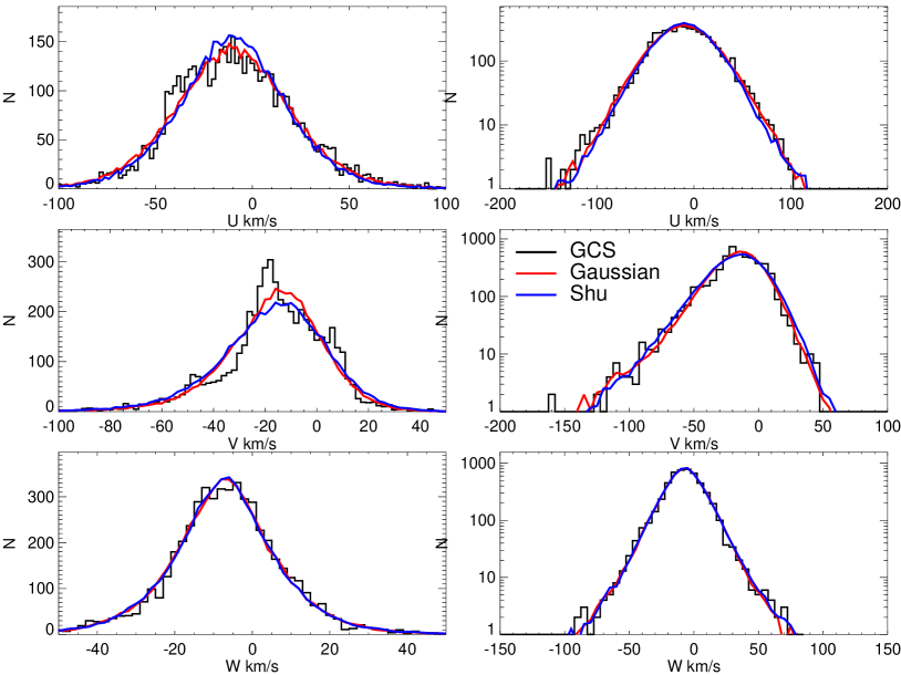
Figure 5.— Comparison of model velocity distributions with that of GCS data. The right panels differ from the left only in range and scale of axes. The model used is the best fit Gaussian (column 1 of Table 7) and the Shu model (column 1 of Table 7) for the GCS data. Both the models are acceptable fits to the data. Significant structures can be seen in the velocity space.

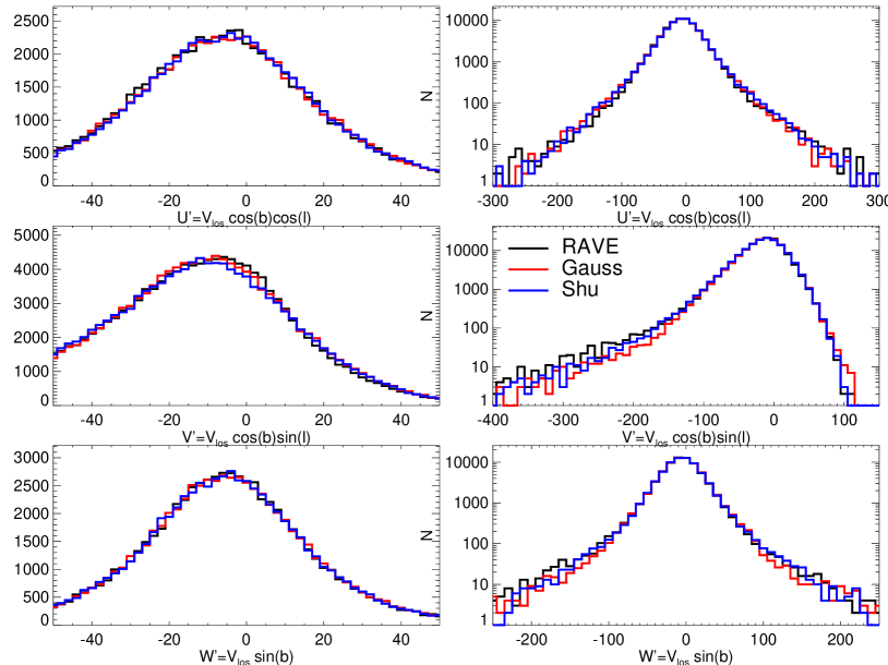
Figure 6.— Comparison of model velocity distributions with that of RAVE data. Projection of radial velocity along $U,V$ and $W$ directions are shown. The right panels differ from the left only in range and scale of axes. The top panel is for stars with $(|b|<45)\&((|l|>45)||(|l-180|>45))$, the middle panel is for stars with $(|b|<45)\&((|l|<45)\/||(|l-180|<45))$ and the bottom panel is for stars with $|b|>45$. The model used is the best fit Gaussian (column 5 in Table 7) and the Shu model (column 6 of Table 7) for the RAVE data. The Shu model clearly models the wings of $V^{\prime}$ better than the Gaussian model, especially in region $-200$ km s^-1 $<V^{\prime}<-150$ km s^-1 and $V^{\prime}>80$ km s^-1 which is dominated by thick disc. A slight mismatch at $V^{\prime}\sim 0$ is also seen.

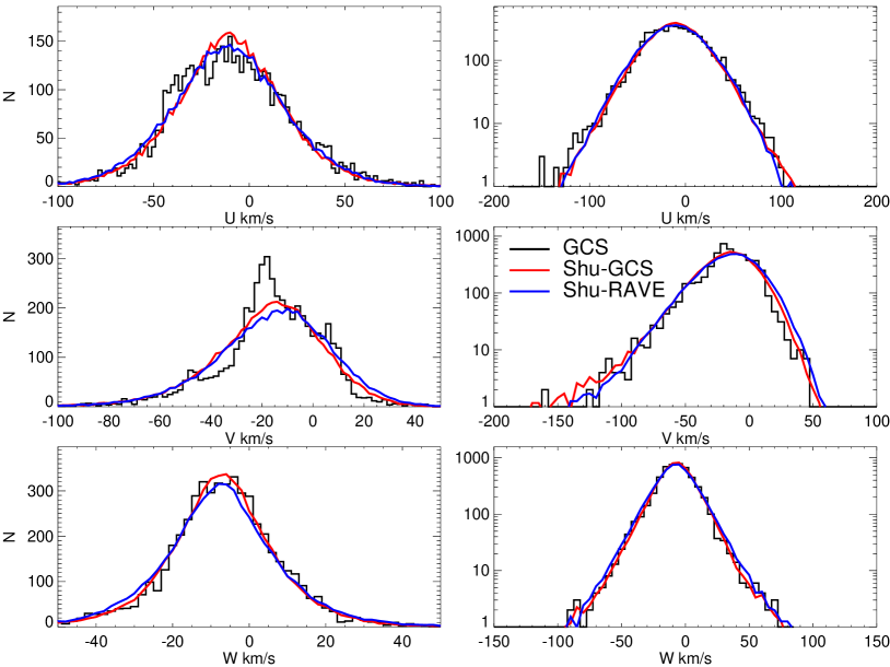
Figure 7.— Comparison of model velocity distributions with that of GCS data. The models used correspond to columns 2 and 6 of Table 7. These are Shu models that a) best fit the GCS data but with a few parameters fixed and b) best fit the RAVE data. The positive wing of $V$ is slightly overestimated by the RAVE best fit model.

6. Discussion

6.1. Correlations and degeneracies

Not all parameters are independent. The dominant correlations are shown in Figures 10, 11, 12 and 13 where pairwise posterior distributions of parameters are plotted. The implication of any correlation is that a change in one of the values also changes the other value without affecting the quality of the fit. In other words, a precise value of one correlated quantity needs to be known in order to determine the other. We find that the $\beta$ values are strongly correlated with the corresponding $\sigma^{\rm thin}$ values. This is mainly because we do not have enough information in the data to estimate the ages of stars. The model specifies the prior on the ages of stars and the data gives the velocities. The degeneracy reflects the fact that during fitting $\beta$ can be adjusted while keeping the mean velocity dispersion constant.

In both thin and thick discs $\sigma_{R}$ is correlated with $R_{\sigma}$. These correlations are stronger for the Shu model than the Gaussian model. To get a good estimate of $R_{\sigma}$ ideally one would require a sample of stars distributed over a large volume. In the absence of an extended sample, the constraint on $R_{\sigma}$ comes from the fact that it also determines the $v_{\phi}$ distribution. The amount of asymmetric drift increases with $\sigma_{R}$ and decreases with $R_{\sigma}$ (see Equation (6)). If the asymmetric drift is fixed, this naturally leads to the correlation between $R_{\sigma}$ and $\sigma_{R}$. In the Shu model the effective velocity dispersion $\sqrt{\langle v_{R}^{2}\rangle}$ is not only proportional to $\sigma_{R}$ but also decreases with $R_{\sigma}$. So one can keep the effective velocity dispersion constant by decreasing both $R_{\sigma}$ and $\sigma_{R}$ at the same time. This makes the correlation in Shu model stronger.

Also, $V_{\odot}$ is correlated with $R_{\sigma}^{\rm thin}$ and this relation is stronger for the Gaussian model. This makes it difficult to determine $V_{\odot}$ and $R_{\sigma}$ reliably using the Gaussian models. The Shu model does not have this problem because in it the azimuthal motion is coupled to the radial motion, so it has three fewer parameters, i.e., has fewer degrees of freedom. This helps to resolve the $R_{\sigma}^{\rm thin}-V_{\odot}$ degeneracy.

When fitting Shu models to RAVE we find an anti-correlation exists between thin and thick disc parameters, e.g., $(\sigma^{\rm thin}_{R},\sigma^{\rm thick}_{R})$, $(\sigma^{\rm thin}_{z},\sigma^{\rm thick}_{z})$ and $(R_{\sigma}^{\rm thin},R_{\sigma}^{\rm thick})$. This is mainly because we do not have any useful information about the ages of stars.

We now discuss the parameters $\Theta_{0}$ and $\alpha_{z}$ which were free only for RAVE data. The value of $\alpha_{z}$ is correlated with $\Theta_{0}$ and anti-correlated with $V_{\odot}$. The $\Theta_{0}$ parameter is anti-correlated with both $U_{\odot}$ and $R_{\sigma}^{\rm thin}$. For the GCS data, the $(\Theta_{0},R_{\sigma}^{\rm thin})$ correlation is so strong that it is difficult to get meaningful constraints on $\Theta_{0}$ so the later was fixed.

6.2. Solar peculiar motion

Among the three components of Solar motion, $U_{\odot}$ and $W_{\odot}$ are only weakly correlated with other variables and give similar values for both Gaussian and Shu models. The only major dependence of $U_{\odot}$ is for RAVE, where it is anti-correlated with $\Theta_{0}$ by about $-0.5$. So models with $\alpha_{z}=0$ that underestimate $\Theta_{0}$, will overestimate $U_{\odot}$. For RAVE we get $W_{\odot}=7.54\pm 0.1\,{\rm km}\,{\rm s}^{-1}$ and $U_{\odot}=10.96\pm 0.14\,{\rm km}\,{\rm s}^{-1}$ (column 6 of Table 7). GCS values for $W_{\odot}$ and $U_{\odot}$ are lower by about 0.4 and 0.8 km s^-1 respectively but their $3-\sigma$ range matches with RAVE (column 2 of Table 7). The small mismatch could be either due to large-scale gradients in the mean motion of stars (Williams et al., 2013) in RAVE or due to kinematic substructures in GCS.

Our GCS results (column 2 of Table 7) are in excellent agreement with Dehnen & Binney (1998b), but differ from Schönrich et al. (2010) for $U_{\odot}$ by 1.0 km s^-1. Nevertheless, $U_{\odot}$ is well within their quoted $2\sigma$ range. The RAVE $U_{\odot}$ agrees with Schönrich et al. (2010). Interestingly, with the aid of a model-independent approach, Schönrich (2012) finds from SDSS stars $U_{\odot}=14.0\pm 0.3$ km s^-1 but with a systematic uncertainty of 1.5 km s^-1. The systematic errors in distances and proper motion can bias this result. Additionally, the analyzed sample not being local, his results can also be biased if there are large-scale streaming motions.

We now discuss our results for $V_{\odot}$. For Gaussian models the estimated $V_{\odot}$ value depends strongly on the choice of $R_{\sigma}$ values and it is difficult to get a reliable value for either of them. For the Shu model, $V_{\odot}$ depends on whether $\alpha_{z}$ is fixed, in fact they are anti-correlated (see LABEL:rave_shu). For $\alpha_{z}=0$, the GCS and RAVE $V_{\odot}$ agree with each other, but when $\alpha_{z}$ is free, $V_{\odot}$ is $2\,{\rm km}\,{\rm s}^{-1}$ lower from RAVE than from GCS (columns 2 and 6 of Table 7). The $\alpha_{z}=0$ model not only has a higher $\chi_{\rm red}^{2}$ but, as we will discuss later, also yields a low value of $\Theta_{0}$, so we consider this model less useful. The most likely cause for the difference between RAVE and GCS $V_{\odot}$ is the significant amount of kinematic substructures in the distribution of the $V$ component of the GCS velocities (LABEL:gcs_UVW4). It can be seen in LABEL:gcs_UVW4 that the best fit RAVE model, in spite of apparently having low $V_{\odot}$, is still a good description of the GCS data. Moreover, in GCS a dominant kinematic structure can be seen at $V\sim-20\,{\rm km}\,{\rm s}^{-1}$ (the Hyades and the Pleiades), lending further support to the idea that GCS probably overestimates $V_{\odot}$. However, this can also be because our formulation for the vertical dependence of kinematics is not fully self consistent (see Section 2.4 and 6.8).

The need to revise $V_{\odot}$ upwards from the value of $5.2$ km s^-1 given by Dehnen & Binney (1998b) has been extensively discussed (Binney, 2010; McMillan & Binney, 2010; Schönrich et al., 2010). Binney (2010) suggests a value of $11.0$ km s^-1 after randomizing some of the stars to reduce the impact of streams while Schönrich et al. (2010) get $V_{\odot}=12.24\pm 0.47$ km s^-1. Our RAVE value of $V_{\odot}=7.5\pm 0.2$ is significantly lower that this (column 6 of Table 7). Our GCS value of $V_{\odot}=9.8\pm 0.3$ km s^-1 is also lower than both of them (column 2 of Table 7).

Recently, Golubov et al. (2013) determined $V_{\odot}=3.06\pm 0.68$ by binning the local RAVE stars in color and metallicity bins and applying an improved version of the Stromberg relation. Their estimate is even lower than that of Dehnen & Binney (1998b). The application of the Stromberg relation demands the identification of subpopulations that are in dynamical equilibrium and have the same value for the slope in the relation. Binning by color fails to satisfy these requirements for the reasons given by Schönrich et al. (2010). Golubov et al. do split their sample by metallicity as well as color, but the metallicities are quite uncertain and the bins are quite broad, so a bias due to the selected subpopulations not obeying the same linear relation can be expected.

The discrepancy for the GCS with Schönrich et al. (2010) could be either due to differences in fitting methodologies or differences in the models adopted, with the latter being the most likely cause. The model used here and by Schönrich et al. (2010) is based on the Shu distribution function but still there are some important differences. We have a separate thick disc while in their case the thick disc arises naturally due to radial mixing. The forms of $\sigma_{R}(L)$ and $\Sigma(L)$ also differ ($L$ being angular momentum). Our form of $\sigma_{R}(L)$ is the same as that used by Binney (2010) while Schönrich et al. (2010) compute $\sigma_{R}(L)$ so as to satisfy $\langle v_{R,{\rm thin}}^{2}\rangle\propto{\rm e}^{-R/1.5R_{d}}$. In our case $\langle v_{R,{\rm thin}}^{2}\rangle(R)$ depends implicitly upon $R_{\sigma}$ and $\beta$ and both of these parameters are constrained by data. The $\Sigma(L)$ in Schönrich et al. (2010) comes from a numerical simulation involving the processes of accretion, churning and blurring while in our case it comes directly from the constraint that $\Sigma(R)\propto\exp(-R/R_{d})$. The prescription for metallicity in Schönrich et al. (2010) is also very different from ours.

6.3. The circular speed

In a recent paper, Bovy et al. (2012d) used data from the APOGEE survey and analyzed stars close to the mid-plane of the disc to find $\Theta_{0}=218\pm 6$ km s^-1 and $V_{\odot}=26\pm 3\,{\rm km}\,{\rm s}^{-1}$. The resulting angular velocity $\Omega_{\odot}=(\Theta_{0}+V_{\odot})/R_{0}$ agrees with the value of $30.24\pm 0.11\,{\rm km}\,{\rm s}^{-1}\,{\rm kpc}^{-1}$ as estimated by Reid & Brunthaler (2004) using the Sgr A* proper motion or as estimated by McMillan & Binney (2010) using masers ($\Omega_{\odot}$ in range $29.9-31.6\,{\rm km}\,{\rm s}^{-1}\,{\rm kpc}^{-1}$). However, Bovy et al. (2012d) found that $V_{\odot}$ is about $14\,{\rm km}\,{\rm s}^{-1}$ larger than the value measured in the solar neighborhood by GCS. As a way to reconcile their high $V_{\odot}$, Bovy et al. (2012d) suggest that the LSR itself is rotating with a velocity of $\sim 12\,{\rm km}\,{\rm s}^{-1}$ with respect to the RSR (rotational standard of rest as measured by circular speed in an axis-symmetric approximation of the full potential of the Milky Way).

For RAVE data, we get $\Theta_{0}=232\pm 1.7\,{\rm km}\,{\rm s}^{-1}$ and $\Omega_{\odot}=29.9\pm 0.3\,{\rm km}\,{\rm s}^{-1}\,{\rm kpc}^{-1}$ which agrees with the proper motion of Sgr A*, $30.24\pm 0.1\,{\rm km}\,{\rm s}^{-1}\,{\rm kpc}^{-1}$. Hence, the RAVE data suggest that the LSR is on a circular orbit and is consistent with RSR. Our value $\alpha_{z}=0.047$ is slightly higher than the value $0.0374$ predicted by analytical models of the Milky Way potential LABEL:vcirc_z. This is expected because in our formalism, the parameter $\alpha_{z}$ also contributes to the decrease in mean rotation speed with height. If we explicitly put a prior on $\Omega_{\odot}$, then we have the liberty of constraining one more parameter and we use it to constrain the radial gradient of circular speed $\alpha_{R}$. Doing so, we find a small gradient of about $0.67\,{\rm km}\,{\rm s}^{-1}\,{\rm kpc}^{-1}$ (column 7 of Table 7) and $\Theta_{0}$ increases to $235\,{\rm km}\,{\rm s}^{-1}$.

We find that the parameter $\alpha_{z}$ that controls the vertical dependence of circular speed plays an important role in determining $\Theta_{0}$. For models with $\alpha_{z}=0$, $\Theta_{0}$ is underestimated and we end up with $\Theta_{0}=212\pm 1.4$. This is in rough agreement with Bovy et al. (2012d) but $V_{\odot}$ is not. The resulting angular velocity $\Omega_{\odot}$ is also much lower than the value obtained from the proper motion of Sgr A*. If, on the contrary, $\alpha_{z}$ is free, we automatically match the proper motion of Sgr A* and we get a value of $V_{\odot}$ that is similar to that from the local GCS sample.

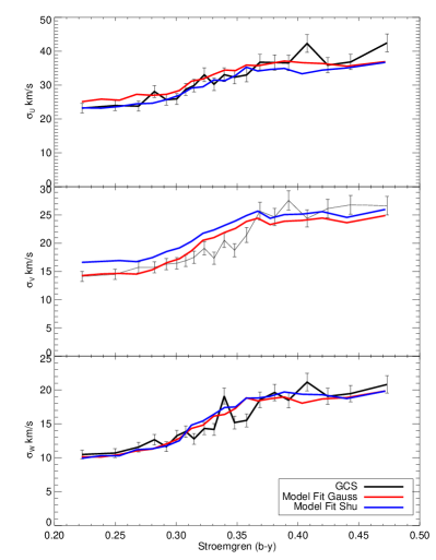
Figure 8.— Velocity as a function of $b-y$ Strömgren color for GCS stars. The error bars were estimated from Poisson noise. Shown alongside are predictions from various models. Note, the color distribution was not taken into account when fitting models to data.

6.4. The age-velocity dispersion relation (AVR)

We now discuss our model predictions for the age velocity dispersion relation in the thin disc, specifically the parameters $\beta_{z},\beta_{\phi},\beta_{R}$, $\sigma_{z}^{\rm thin},\sigma_{\phi}^{\rm thin}$ and $\sigma_{R}^{\rm thin}$. We find $\beta_{R}<\beta_{\phi}<\beta_{z}$. The GCS $\beta_{R,\phi,z}$ values were similar for both Gaussian and Shu models. The RAVE value of $\beta_{R}$ from the Shu model, also agrees with these GCS values. The value of $\beta_{z}$ is difficult to determine precisely with RAVE, so, we used the corresponding GCS value in the fits. The values of $\beta_{R,\phi}$ from RAVE with the Gaussian model are systematically lower than the GCS values. Since the RAVE Gaussian model did not fit the data well, we give less importance to its $\beta$ values and ignore them for the present discussion. Overall, results in column 1 of Table 7 provide a good representation of our predictions and are shown alongside literature values in Table 8.

Our values of $\beta$ and the velocity dispersion in the Solar neighborhood for 10 Gyr old stars, $\sigma_{R,\phi,z}^{\rm thin}$, depend on whether the thick disc is considered a distinct component: when only one component is provided, so the thick disc has to be accommodated by the old tail of the thin disc, these quantities are naturally higher (column 2 of Table 7). The values we recover for $\sigma_{R,\phi,z}^{\rm thin}$ are very similar regardless of which survey or which model we employ.

We now compare our results with previous estimates. In the Besançon model, the age-velocity dispersion relation for the thin disc was based on an analysis of Hipparcos stars by Gomez et al. (1997). Sharma et al. (2011) fitted their tabulated values using analytical functions and the values are given in Table 5. Nordström et al. (2004) used their ages for individual GCS stars to find $(\beta_{R},\beta_{\phi},\beta_{z})=(0.31,0.34,0.47)$. Seabroke & Gilmore (2007), using the same data, concluded that the error bars need enlarging and pointed out that excluding the Hercules stream increases $\beta_{z}$ to 0.5. Holmberg et al. (2007) and Holmberg et al. (2009) updated the data with new parallaxes and photometric calibrations and found $(\beta_{R},\beta_{\phi},\beta_{z})=(0.39,0.40,0.53)$. By contrast, Just & Jahreiß (2010) used a selection of Hipparcos stars and an elaborate model of the solar cylinder to estimate $\beta_{z}=0.375$. Aumer & Binney (2009) analyzed revised Hipparcos data with a refinement of the approach of Binney et al. (2000). Their analysis used only the variation with color of velocity dispersion and number density; they did not use age estimates for individual stars. The advantage of this approach is that one can include main-sequence stars with colors that span a much wider range than the GCS catalogue does. The disadvantage is that only proper motions can be used. They found $(\beta_{R},\beta_{\phi},\beta_{z})=(0.307,0.430,0.445)$. Since they did not distinguish the thick disc, their $\beta$ values are closer to the values ($0.268,0.349,0.432$) we obtain without a thick disc. For the velocity dispersions, however, Aumer & Binney (2009) find $(\sigma_{R}^{\rm thin},\sigma_{\phi}^{\rm thin},\sigma_{z}^{\rm thin})=(41.90,28.82,23.83)$, which agree better with our values when we include a thick disc.

As (Table 8) shows, our values for $\beta$ are slightly lower than those from previous studies when we do not include a thick disc, and significantly lower when a thick disc is included. While uncertainty in ages remains a big worry in the analysis of Holmberg et al. (2009), the difference between our results with those of Aumer & Binney (2009) is most likely due to different methods. The main differences being that we use many fewer stars stars and we use line-of-sight velocities rather than proper motions. Also the density laws assumed for the distribution of stars in space are different. In LABEL:gcs_colvel we show the velocity dispersion as a function of Strömgren $b-y$ color. Although we have not used this color, our fitted model correctly reproduces dispersion as a function of color. The Shu model is found to overpredict $\sigma_{V}$ for $(b-y)<0.35$ but only slightly.

Table 8 Comparison of values of $\beta$ as estimated by different sources

Source	$\beta_{R}$	$\beta_{\phi}$	$\beta_{z}$
Fit to Robin et al. (2003)	0.33	0.33	0.33
Nordstrom et al. (2004)	$0.31\pm 0.05$	$0.34\pm 0.05$	$0.47\pm 0.05$
Seabroke & Gilmore (2007)			$0.48\pm 0.26$
Holmberg et al. (2007)	0.38	0.38	0.54
Holmberg et al. (2009)	0.39	0.40	0.53
Aumer & Binney (2009)	0.307	0.430	0.445
Just and Jahreiss (2010)			0.375
Our GCS Thin only	$0.27\pm$0.02	0.35$\pm$0.02	0.43$\pm$0.02
Our GCS Thin+Thick	0.20$\pm$0.02	0.27$\pm$0.02	0.36$\pm$0.02
Our RAVE Thin+Thick	0.19$\pm$0.01		0.3-0.4

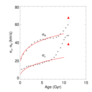
Figure 9.— Comparison of our age-velocity dispersion relation (solid line) with that of Minchev et al. (2013) (black points). The slopes used are $\beta_{z}=0.37$ and $\beta_{R}=0.23$ for $\sigma_{R}=50.0$ and $\sigma_{z}=24.0$. The triangles are for the thick disc in our Gaussian models for GCS.

The ratio of $\sigma_{z}/\sigma_{R}$ and the $\beta_{i}$ values are useful for understanding the physical processes responsible for heating the disc. Spitzer & Schwarzschild (1953) first showed that scattering of stars by gas clouds can cause velocity dispersion to increase with age. This process was extensively analysed by Binney & Lacey (1988), but they predicted a value of $\sigma_{z}/\sigma_{R}$ from cloud scattering that is too large because they assumed that an isotropic distribution of star-cloud impact parameters. When the anisotropy of impact parameters is taken into account, in the steady state $\sigma_{R}/\sigma_{z}=0.62$. (Ida et al., 1993; Shiidsuka & Ida, 1999; Sellwood, 2008). Hänninen & Flynn (2002) showed that with giant molecular clouds one gets $\beta_{R}=0.2$ and $\beta_{z}=0.25$, compared to our favoured values $\beta_{R}=0.20$, $\beta_{z}=0.36$. However, the population of massive gas clouds is not numerous enough to account for the measured acceleration of thin-disc stars – the role of clouds must be to convert random motion in the plane into random motion vertically (Jenkins, 1992; Hänninen & Flynn, 2002).

Lacey & Ostriker (1985) and Hänninen & Flynn (2002) have investigated scattering by $\sim 10^{7}M_{\odot}$ halo objects such as black holes and find then that $\beta_{R,z}\sim 0.5$ and that $\sigma_{z}/\sigma_{R}$ lies between 0.40 and 0.67. Massive halo objects act differently from GMCs for several reasons: they are not confined to the disc, they are on highly non-circular orbits, and they have large escape velocities, so they can scatter through large angles.

For RAVE, from either the Gaussian or Shu models, we get $\sigma_{z}^{\rm thin}/\sigma_{R}^{\rm thin}~{}0.65$ (column 6 of Table 7 and column 6 of Table 7). The corresponding GCS value is 0.58 (column 3 of Table 7 and column 2 of Table 7). Models without a thick disc give a similar value for $\sigma_{z}/\sigma_{R}$. These are values for a 10 Gyr old population and we think they agree well with the above predictions. For the thick disc we find that the Gaussian model predicts $\sigma_{z}^{\rm thick}/\sigma_{R}^{\rm thick}=0.68$, while the Shu model predicts a higher value, 0.80.

Heating by cloud scattering predicts $\beta_{R}\sim\beta_{z}$. Scattering by spiral arms at Lindblad resonances also heats discs. If spiral arms are transient, individual resonances are broad, and over the life of the disc one or more resonances is likely to have affected every region of the disc. Spirals only increase in-plane dispersions (Carlberg & Sellwood, 1985; Binney & Lacey, 1988; Sellwood, 2013). The predicted values of $\beta_{R}$ are between 0.2 for high-velocity stars and 0.5 for low-velocity stars. Multiple spiral density waves (Minchev & Quillen, 2006) or a combination of bar and spirals can also heat up the disc (Minchev & Famaey, 2010). When the $\beta_{i}$ differ from one another, as we find, the axial ratios of the velocity ellipsoid are functions of age. If $\beta_{z}>\beta_{R}$, $\sigma_{z}/\sigma_{R}$ increases with age as $\tau^{\beta_{z}-\beta_{R}}$, so it is much lower for younger stars. Aumer & Binney (2009) also find that $\sigma_{z}/\sigma_{R}$ increases with age and remark that this trend is consistent with scattering by spiral arms playing a significant role for young stars.

Recently, Minchev et al. (2013) investigated the age-velocity dispersion relation for stars in simulations of disc galaxies and find it to be in rough agreement with observations. We now compare our results with their findings. In LABEL:minchev_sigma, we plot their predictions for $\sigma_{R}$ and $\sigma_{z}$ for stars in a Solar cylinder defined by $7<R<9$ kpc. The red curves show our AVR from Equation (9) with $\beta_{z}=0.37$ and $\beta_{R}=0.23$, values that fit both the RAVE and GCS data well when using the Shu model (column 2 of Table 7). It can be seen that for ages less than 7 Gyr, the adopted $\beta$ values correctly reproduce the profiles seen in simulations. However, the simulations require a smaller value $\sigma_{z}/\sigma_{R}\sim 0.5$ than the data require, and the red curves in LABEL:minchev_sigma have been individually scaled to fit the simulations. Hence, although the normalization constant $\sigma_{z}^{\rm thin}$ is roughly in agreement with our results for the Galaxy, the normalization constant $\sigma_{R}^{\rm thin}$ is too high by about $10\,{\rm km}\,{\rm s}^{-1}$. There is a slight hint that in the simulations $\sigma_{R}$ flattens beyond 5 Gyr, but it is also consistent with our power law prescription. Since the simulation data are for $7<R<9$ kpc, and the density of stars and the velocity dispersion increases inwards, the dispersions in the simulations are expected to be slightly high compared to dispersions at $R=R_{0}$. In our model the thin disc started forming 10 Gyr ago (solid line) and stars older than this belong to the thick disc with a constant age of 11 Gyr (shown by red triangles). This is an effective if rather crude representation of what is found in the simulations.

6.5. The thick disc

First, we discuss our results for the Gaussian model. Our values for $(\sigma_{R}^{\rm thick},\sigma_{\phi}^{\rm thick},\sigma_{z}^{\rm thick})$ for the thick disc from fitting the Gaussian model to GCS (column 3 of Table 7) are in good agreement with results of Soubiran et al. (2003) ($39\pm 4,39\pm 4,63\pm 6$) but differ from those of Robin et al. (2003) regarding $\sigma_{\phi}^{\rm thick}$. The RAVE $\sigma_{R}^{\rm thick}$ is lower than GCS by $7\,{\rm km}\,{\rm s}^{-1}$ (column 6 of Table 7) but the other dispersions match up with GCS.

In the Gaussian model the thick disc velocity dispersions are much larger than those of the old thin disc. In the Shu models, we find that the thick disc dispersions are very similar to the old thin disc (column 6 of Table 7). However, $R_{\sigma}^{\rm thick}$ is much shorter than $R_{\sigma}^{\rm thin}$. The Gaussian and Shu models differ in their estimates for the thick disc velocity dispersions for the following reason. In the Shu model, the parameter $\sigma_{R}^{2}$, which controls the velocity dispersion, is a function of age $\tau$ and guiding radius $R_{g}$ and is not equal to the velocity dispersion $\overline{v_{R}^{2}}(\tau,R)$. For a positive $R_{\sigma}$, $\overline{v_{R}^{2}}(\tau,R)=\int\sigma_{R}^{2}(\tau,R_{g})P(R_{g}|R,\tau)dR_{g}>\sigma_{R}^{2}(\tau,R_{g}=R)$. In a warm disc there are generally a significant number of stars with $R_{g}<R$ at radius $R$. Decreasing $R_{\sigma}$ not only makes stars at small radii hotter, but also makes them more likely to be found at $R>R_{g}$, so decreasing $R_{\sigma}$ increases $\overline{v_{R}^{2}}(\tau,R)$. For the set of parameters given in column 6 of Table 7, we find that at $R=R_{0}$

$$\sqrt{\langle v_{z,{\rm thin}}^{2}\rangle(\tau)} = 26.8\left(\frac{\tau+0.1}{10.1\,{\rm Gyr}}\right)^{0.41}\,{\rm km}\,{\rm s}^{-1}$$ (33)

$$\sqrt{\langle v_{R,{\rm thin}}^{2}\rangle(\tau)} = 41.4\left(\frac{\tau+0.1}{10.1\,{\rm Gyr}}\right)^{0.22}\,{\rm km}\,{\rm s}^{-1}$$ (34)

$$\sqrt{\langle v_{z,{\rm thick}}^{2}\rangle} = 40.0\,{\rm km}\,{\rm s}^{-1},$$ (35)

$$\sqrt{\langle v_{R,{\rm thick}}^{2}\rangle} = 49.4\,{\rm km}\,{\rm s}^{-1},$$ (36)

with $0<\tau<10\,{\rm Gyr}$. So the total thick disc $\overline{v_{z,R}^{2}}$ in the solar neighborhood is still much larger than that of the thin-disc.

In the Shu model the dispersions at $R_{g}=R_{0}$ of the old thin disc and the thick disc are similar, consistent with the thick disc being merely the tail of the thin disc. Moreover, although $R_{\sigma}^{\rm thick}$ is much smaller than $R_{\sigma}^{\rm thin}$, we cannot at this stage exclude a smooth decrease in $R_{\sigma}$ with age. Additionally, our prior on age and distance distribution assumes a distinct thick disc, e.g., in LABEL:rave_stat1 it can be seen that the distance distribution changes suddenly at $10\,{\rm Gyr}$. This could be responsible for $R_{\sigma}^{\rm thick}$ being shorter than $R_{\sigma}^{\rm thin}$, perhaps because all scale lengths decrease with age as Bovy et al. (2012c) infer.

Table 9 Constraints on model parameters with Bovy et al. (2012d) Gaussian model. See Table 7 for further description.

Model	RAVE BOVY	RAVE BOVY	RAVE BOVY	RAVE BOV
$U_{\odot}$	$10.16_{-0.15}^{+0.15}$	$11.78_{-0.15}^{+0.15}$	$11.59_{-0.14}^{+0.15}$	$10.96_{-0.14}^{+0.14}$
$V_{\odot}$	$13.36_{-0.22}^{+0.25}$	$6.2_{-0.18}^{+0.18}$	$8.77_{-0.28}^{+0.28}$	$0.032_{-0.024}^{+0.052}$
$W_{\odot}$	$7.364_{-0.098}^{+0.098}$	$7.688_{-0.09}^{+0.09}$	$7.694_{-0.089}^{+0.097}$	$7.622_{-0.087}^{+0.094}$
$\sigma_{\phi}^{\rm thin}$	$26.455_{-0.096}^{+0.095}$	$33.11_{-0.27}^{+0.29}$	$25.83_{-0.38}^{+0.36}$	$33.84_{-0.27}^{+0.28}$
$\sigma_{R}^{\rm thin}$	$41.39_{-0.16}^{+0.17}$	$57.58_{-0.31}^{+0.31}$	$41.55_{-0.62}^{+0.57}$	$51.44_{-0.27}^{+0.29}$
$\sigma_{z}^{\rm thin}$	$22.99_{-0.12}^{+0.12}$	$31.55_{-0.3}^{+0.3}$	$23.29_{-0.62}^{+0.6}$	$33.6_{-0.29}^{+0.29}$
$\sigma_{\phi}^{\rm thick}$			$37.45_{-0.56}^{+0.5}$
$\sigma_{R}^{\rm thick}$			$65.69_{-0.64}^{+0.55}$
$\sigma_{z}^{\rm thick}$			$38.84_{-0.52}^{+0.47}$
$\beta_{R}$	$0.01$	$0.4584_{-0.0066}^{+0.0071}$	$0.193_{-0.012}^{+0.013}$	$0.3568_{-0.0049}^{+0.0045}$
$\beta_{\phi}$	$0.01$	$0.3747_{-0.009}^{+0.0093}$	$0.166_{-0.013}^{+0.013}$	$0.4151_{-0.0093}^{+0.0081}$
$\beta_{z}$	$0.01$	$0.514_{-0.013}^{+0.016}$	$0.263_{-0.027}^{+0.025}$	$0.588_{-0.016}^{+0.013}$
$1/R_{\sigma}^{\rm thin}$	$-0.029_{-0.0035}^{+0.003}$	$0.0493_{-0.0024}^{+0.0026}$	$0.0116_{-0.005}^{+0.0051}$	$0.0418_{-0.0031}^{+0.0028}$
$1/R_{\sigma}^{\rm thick}$			$0.069_{-0.0039}^{+0.0038}$
$\Theta_{0}$	$210.8_{-1.5}^{+1.5}$	$205.5_{-1.5}^{+1.5}$	$213.9_{-1.6}^{+1.6}$	$239.1_{-1.9}^{+1.7}$
$k_{\rm ad}$	$0.85$	$0.85$	$0.85$	$1.968_{-0.021}^{+0.022}$

6.6. The radial gradient of velocity dispersions

To date, there has been little discussion in the literature about the parameter $R_{\sigma}$ that controls the radial dependence of velocity dispersion. This choice of the radial dependence is motivated by the desire to produce discs in which the scale height is independent of radius. For example, under the epicyclic approximation, if $\sigma_{z}/\sigma_{R}$ is assumed to be constant, then the scale height is independent of radius for $R_{\sigma}=2R_{d}$ (van der Kruit & Searle, 1982; van der Kruit, 1988; van der Kruit & Freeman, 2011). Lewis & Freeman (1989) using 600 old disc K giants spanning 1 to 17 kpc in galactocentric radius estimate $R_{\sigma}$ to be $8.7\,{\rm kpc}$ for radial velocity and $6.7\,{\rm kpc}$ for azimuthal velocity. Ojha et al. (1996) using a survey of UBVR photometry and proper motions in different directions of the Galaxy estimated $R_{\sigma}=11\pm 1.6\,{\rm kpc}$. Bovy et al. (2012b) using SDSS/SEGUE data find $R_{\sigma}=7.1\,{\rm kpc}$ for vertical velocity dispersions. Bovy et al. (2012d) using APOGEE data find $R_{0}/R_{\sigma}$ to be between -0.24 to 0.03, for the radial and azimuthal motion. In our modelling, the radial gradient is assumed to be same for all the three components.

Our results indicate that for GCS, $R_{\sigma}$ is positive for both Gaussian and Shu models. In the case of RAVE, the Shu model yields $R_{\sigma}\sim 14\,{\rm kpc}$ but the Gaussian model requires $R_{\sigma}$ to be negative. Moreover, we find that when the Gaussian model used by Bovy et al. (2012d) is fitted to the RAVE data, $R_{\sigma}$ is again negative: $R_{\sigma}^{\rm thin}=-34\,{\rm kpc}$ (column 1 of Table 9), similar to their result $(-0.24<R_{0}/R_{\sigma}<0.03)$. Since the Shu model also fits the data better, we think that negative values of $R_{\sigma}$ obtained with Gaussian models are spurious. The Gaussian model does not fit the RAVE data well because in a warm disc the $v_{\phi}$ distribution is very skew, and the Shu DF correctly handles the asymmetry. Moreover, the $R_{\sigma}^{\rm thin}$ estimate from the Shu model agrees for both GCS and RAVE, lending further support to the proposition that the problem is related to the use of the Gaussian model.

Positive $R_{\sigma}$ agrees with the findings of Lewis & Freeman (1989). It should be noted that in both our analysis and that of Bovy et al. (2012d), the value of $R_{\sigma}$ is strongly influenced by how the asymmetric drift is modelled. On the other hand, the values reported by Lewis & Freeman (1989) are a direct measure of the radial gradient of velocity dispersion. From RAVE data, the thick disc’s value of $R_{\sigma}$ is in general higher than the thin disc’s value.

Table 10 Investigation of systematics.

Model	RAVE SHU	RAVE SHU	RAVE SHU	RAVE SHU	RAVE SHU	RAVE SHU	RAVE SHU
Distance Change					90%	110%
$U_{\odot}$	$10.96_{-0.13}^{+0.14}$	$11.05_{-0.16}^{+0.15}$	$10.81_{-0.14}^{+0.15}$	$10.98_{-0.15}^{+0.14}$	$11.01_{-0.14}^{+0.13}$	$10.82_{-0.14}^{+0.15}$	$10.71_{-0.14}^{+0.14}$
$V_{\odot}$	$7.53_{-0.16}^{+0.16}$	$7.62_{-0.16}^{+0.13}$	$7.39_{-0.14}^{+0.14}$	$7.59_{-0.14}^{+0.16}$	$8.26_{-0.15}^{+0.15}$	$6.81_{-0.16}^{+0.15}$	$7_{-0.16}^{+0.15}$
$W_{\odot}$	$7.539_{-0.09}^{+0.095}$	$7.553_{-0.09}^{+0.086}$	$7.52_{-0.088}^{+0.085}$	$7.535_{-0.089}^{+0.082}$	$7.553_{-0.091}^{+0.078}$	$7.53_{-0.083}^{+0.09}$	$7.517_{-0.088}^{+0.088}$
$\sigma_{R}^{\rm thin}$	$39.67_{-0.72}^{+0.63}$	$39.56_{-0.7}^{+0.66}$	$39.27_{-0.62}^{+0.56}$	$39.45_{-0.61}^{+0.67}$	$39.23_{-0.6}^{+0.74}$	$40.09_{-0.49}^{+0.59}$	$31.2_{-0.14}^{+0.12}$
$\sigma_{z}^{\rm thin}$	$25.73_{-0.21}^{+0.21}$	$25.72_{-0.25}^{+0.23}$	$25.69_{-0.2}^{+0.22}$	$25.67_{-0.23}^{+0.23}$	$25.68_{-0.21}^{+0.25}$	$25.77_{-0.22}^{+0.18}$	$17.57_{-0.12}^{+0.13}$
$\sigma_{R}^{\rm thick}$	$42.43_{-1}^{+0.95}$	$43.23_{-1.1}^{+0.96}$	$42.98_{-0.73}^{+0.86}$	$42.67_{-0.72}^{+0.96}$	$43.51_{-0.82}^{+0.85}$	$41.28_{-0.94}^{+0.71}$	$48.51_{-0.6}^{+0.61}$
$\sigma_{z}^{\rm thick}$	$34.3_{-0.57}^{+0.51}$	$34.48_{-0.53}^{+0.54}$	$34.48_{-0.56}^{+0.58}$	$34.66_{-0.55}^{+0.52}$	$34.8_{-0.6}^{+0.55}$	$33.8_{-0.55}^{+0.55}$	$37.99_{-0.43}^{+0.41}$
$\beta_{R}$	$0.195_{-0.013}^{+0.011}$	$0.192_{-0.013}^{+0.012}$	$0.188_{-0.011}^{+0.01}$	$0.192_{-0.012}^{+0.013}$	$0.188_{-0.013}^{+0.013}$	$0.2018_{-0.0093}^{+0.01}$	$0.01$
$\beta_{z}$	$0.37$	$0.37$	$0.37$	$0.37$	$0.37$	$0.37$	$0.01$
$1/R_{\sigma}^{\rm thin}$	$0.073_{-0.003}^{+0.0037}$	$0.0724_{-0.0031}^{+0.0031}$	$0.0752_{-0.0034}^{+0.0034}$	$0.0721_{-0.0026}^{+0.0028}$	$0.0824_{-0.0031}^{+0.0038}$	$0.0631_{-0.0027}^{+0.0029}$	$0.0983_{-0.0024}^{+0.0034}$
$1/R_{\sigma}^{\rm thick}$	$0.1328_{-0.0051}^{+0.005}$	$0.13_{-0.0046}^{+0.0056}$	$0.1357_{-0.0045}^{+0.004}$	$0.126_{-0.0048}^{+0.0035}$	$0.1356_{-0.0044}^{+0.004}$	$0.1319_{-0.0036}^{+0.005}$	$0.1022_{-0.0034}^{+0.0034}$
$\Theta_{0}$	$231.9_{-1.5}^{+1.4}$	$235.02_{-0.83}^{+0.86}$	$223.3_{-1.4}^{+1.3}$	$242.5_{-1.5}^{+1.6}$	$249.8_{-1.5}^{+1.6}$	$218.9_{-1.4}^{+1.5}$	$237.3_{-1.6}^{+1.7}$
$R_{0}$	$8$	$8$	$7.5$	$8.5$	$8$	$8$	$8$
$\alpha_{z}$	$0.0471_{-0.0019}^{+0.0016}$	$0.0471_{-0.0019}^{+0.0019}$	$0.0532_{-0.0017}^{+0.0017}$	$0.0439_{-0.0017}^{+0.0016}$	$0.0504_{-0.0018}^{+0.0018}$	$0.0462_{-0.0018}^{+0.0016}$	$0.0528_{-0.0019}^{+0.0019}$
$\alpha_{R}$	$0$	$0.67_{-0.26}^{+0.25}$	$0$	$0$	$0$	$0$	$0$

6.7. Comparison with Bovy’s kinematic model

We carried out a more detailed analysis of the kinematic model used by Bovy et al. (2012d). We stress that there are significant differences regarding both data and methodology between the analysis done by us and by Bovy et al. (2012d), and these should be kept in mind when comparing the results. Their sample is close to the plane $|b|<1.5^{\circ}$ and lies in the range $30^{\circ}<\ell<330^{\circ}$. Being close to the plane, they cannot measure vertical motion, but the advantage is they do not have to worry about the dependence of asymmetric drift with vertical height $z$. The $\ell$ and $b$ range being different means that their data and ours probe spatially different regions of the Milky Way. If the disc is axisymmetric, we hope to get similar answers, but not otherwise.

Their main analysis uses a single-population Gaussian model that does not include an age-velocity dispersion relation, so we set $\beta_{R}\sim\beta_{\phi}\sim\beta_{z}\sim 0$. They use a modified formula for the asymmetric drift (Equation 7). In this formula we set the parameter $k_{\rm ad}$ (in the notation of Bovy et al. $X$) to 0.85. Our results are shown in column 1 of Table 9. As mentioned earlier, using RAVE data and a Gaussian model we obtain a negative value of $R_{\sigma}^{\rm thin}=-34\,{\rm kpc}$ just as they do, in consequence of modelling a warm population with a Gaussian model. Our value of $\Theta_{0}$ is also in agreement but our $\sigma_{R}$ is much larger than their value, $31.4\,{\rm km}\,{\rm s}^{-1}$. Their sample could be dominated by cold stars on account of its proximity to the plane. They find $\sigma_{\phi}/\sigma_{R}=0.83$, which is higher by about 0.1 than our ratio for either RAVE or GCS using any type of model.

They also explored multiple populations with a prior on age given by an exponentially declining star formation rate. However, they only quote $\Theta_{0},R_{0}$ and $\sigma_{R}$ for it. For multiple populations, their prior on age for the selected stars ignores the fact that scale height increases with age. This will probably have little impact on $\Theta_{0}$, but their $\sigma_{R}$ values cannot be compared with ours. Also, they assume a priori that $\beta_{R}=\beta_{\phi}=0.38$, but we have shown that $\sigma_{R}$ depends upon the choice of $\beta_{R}$, and when we leave $\beta$ free, we obtain values that differ from 0.38 (column 2 of Table 9). If the thick disc is included, the $\beta$ values are significantly reduced (column 3). In agreement with Bovy et al. (2012d), we find that the value of $\Theta_{0}$ is not affected much by the choice of age-velocity dispersion relation. Including the thick disc leads to an increase in $\Theta_{0}$ by only 8 km s^-1. Interestingly, when $k_{\rm ad}$ is left free, we find the data favor very high values (column 4). This suggests that we are underestimating the asymmetric drift, most probably due to our neglect of the vertical dependence.

6.8. Systematics

Although we get quite precise values for most model parameters, there are additional systematic uncertainties that we have neglected. We performed some additional MCMC runs to investigate these systematics. The results are summarized in Table 10. The first set of systematics is due to two parameters that were kept fixed in our analysis, while the second set is related to our choice of priors on the age and distance distribution of stars.

The distance of the sun from the Galactic center $R_{0}$ and the radial gradient of circular speed $\alpha_{R}$ were kept fixed at 8.0 kpc and zero for most of our analysis. This is because these are strongly correlated with $\Theta_{0}$. Using just the angular position and radial velocity of RAVE stars, it is not possible to constrain them. The effect of changing $R_{0}$ from 7.5 to 8.5 kpc can be seen in column 3 and 4 of Table 10, while the effect of changing $\alpha_{R}$ from zero to $0.65\,{\rm km}\,{\rm s}^{-1}\,{\rm kpc}^{-1}$ can be gauged by comparing columns 1 and 2 in the same table. Using these tables, if needed one can obtain values for any given $R_{0}$ and $\alpha_{R}$ by linearly interpolating between the respective columns. Increasing $\alpha_{R}$ increases $\Theta_{0}$, while the other parameters are relatively unaffected. Increasing $R_{0}$ increases $\alpha_{z}$ as well as $\Theta_{0}$. Again, there is little change in other parameters. The value of $\Omega_{\odot}$ was found to decrease from $30.8\,{\rm km}\,{\rm s}^{-1}\,{\rm kpc}^{-1}$ at $R_{0}=7.5$ kpc to $29.4\,{\rm km}\,{\rm s}^{-1}\,{\rm kpc}^{-1}$ at $R_{0}=8.5$ kpc. The above relationship tentatively suggests that at $R_{0}\sim 7.92$ one can match the proper motion of Sgr A*. We also checked the effect of setting $\alpha_{z}=0.0374$, the value we expect from analytical models. We found that this makes $\Theta_{0}\sim 229.2\,{\rm km}\,{\rm s}^{-1}$ and $V_{\odot}\sim 8.0$, which is not significantly far from the value we get when $\alpha_{z}$ is free.

We now discuss systematics related to our choice of priors. Our main prior is that the age and distance distribution of stars along a particular line of sight is in accordance with the Besançon model of the Galaxy. Additionally, the distance distribution for a given $I_{\rm DENIS}$ magnitude of a star depends upon the isochrones that are used in the model. As a crude way to gauge the sensitivity to our priors in age, we run a model with $\beta_{z}=\beta_{R}=0.01$ (column 7) which makes the kinematics of the thin disc independent of age. As expected, the thin and thick disc parameters change. Other than this, $\alpha_{z}$ and $\Theta_{0}$ are found to increase by 12% and 2% respectively.

Next, we test the effect of changing the distance prior. This could be for example due to a systematic offset in magnitudes predicted by the isochrones. For this we alternately increase and decrease our prior distance distribution by multiplying the distances by a factor of 1.1 and 0.9. The values of $V_{\odot}$, $\Theta_{0}$ and $R_{\sigma}^{\rm thin}$ show significant changes. It should be noted that this is only an approximate way to check the sensitivity of our results on the priors. In reality, if magnitudes predicted by isochrones are systematically wrong then the spatial density model that we use will not match the number count of stars obtained from photometric surveys. So, the mass density laws of the model will have to be modified as well. The proper way to do this is to do a dynamical modelling in which the kinematics and the spatial distribution of stars are fitted jointly to the observational data (e.g. Binney, 2012b).

The biggest source of systematic uncertainty is related to the accuracy of the theoretical models that we use. As discussed earlier in Section 2.4, our treatment of the vertical dependence of the kinematics is not fully self consistent. In reality, for a three dimensional system, the vertical and planar motions are coupled to each other. To model such a system properly one needs a distribution function that incorporates the third integral of motion.

Finally, our models will give rise to errors because they are kinematic rather than dynamical models. Kinematic models offer greater freedom than physics really allows. For example, the parameters $\sigma_{R}$ and $\sigma_{\phi}$ of the Gaussian model are tightly coupled, as are $\beta_{R}$ and $\beta_{\phi}$. The Shu model has fewer free parameters so is less open to this criticism, but it fails to take into account the coupling between the vertical profiles of $\sigma_{R}$ and the mean-streaming velocity $\overline{v}_{\phi}$ (e.g. Binney, 2012a). It is not unreasonable to hope that the values that emerge from the fits for fundamentally superfluous parameters are similar to the values truly mandated by physics, but noise in the data may confound this hope. Clearly, we should proceed as quickly as possible to fitting RAVE with dynamical models like those developed by Binney (2012a).

Table 11 Shu model that best fits the RAVE data (same as column 6 Table 7). Quoted uncertainties are purely random and do not include systematics.

Model	RAVE SHU
$U_{\odot}$	$10.96_{-0.13}^{+0.14}\,{\rm km}\,{\rm s}^{-1}$
$V_{\odot}$	$7.53_{-0.16}^{+0.16}\,{\rm km}\,{\rm s}^{-1}$
$W_{\odot}$	$7.539_{-0.09}^{+0.095}\,{\rm km}\,{\rm s}^{-1}$
$\sigma_{R}^{\rm thin}$	$39.67_{-0.72}^{+0.63}\,{\rm km}\,{\rm s}^{-1}$
$\sigma_{z}^{\rm thin}$	$25.73_{-0.21}^{+0.21}\,{\rm km}\,{\rm s}^{-1}$
$\sigma_{R}^{\rm thick}$	$42.43_{-1}^{+0.95}\,{\rm km}\,{\rm s}^{-1}$
$\sigma_{z}^{\rm thick}$	$34.3_{-0.57}^{+0.51}\,{\rm km}\,{\rm s}^{-1}$
$\beta_{R}$	$0.195_{-0.013}^{+0.011}$
$\beta_{z}$	$0.37$
$1/R_{\sigma}^{\rm thin}$	$0.073_{-0.003}^{+0.0037}{\rm kpc}^{-1}$
$1/R_{\sigma}^{\rm thick}$	$0.1328_{-0.0051}^{+0.005}{\rm kpc}^{-1}$
$\Theta_{0}$	$232.8_{-1.6}^{+1.7}\,{\rm km}\,{\rm s}^{-1}$
$R_{0}$	$8$ kpc
$\alpha_{z}$	$0.0471_{-0.0019}^{+0.0016}$
$\alpha_{R}$	$0.0{\rm\ kpc}^{-1}$

7. Summary and Conclusions

In this paper, we have constrained the kinematic parameters of the Milky Way disc using stars from the RAVE and the GCS surveys. To constrain kinematic parameters, we use analytic kinematic models based on the Gaussian and Shu distribution functions. We use these distribution functions, Padova stellar tracks (Marigo et al., 2008; Bertelli et al., 1994) and the selection functions of the surveys to predict the likelihood of each observed star. For GCS data, which has full phase-space information for the stars, we compute the likelihood in $({\bf x,v})$ phase space. For RAVE data, we choose to fit the likelihood in $(\ell,b,v_{\rm los})$ space to avoid use of uncertain distances and proper motions. We explored the full posterior distribution of model parameters using the Markov Chain Monte Carlo technique. The parameters constrained include the Solar peculiar motion ($U_{\odot},V_{\odot},W_{\odot}$), the circular speed at the Sun $\Theta_{0}$, a parameter $\alpha_{z}$ that controls the vertical gradient of $R\partial\Phi/\partial R$, the age velocity dispersion relations (via $\beta_{R,\phi,z}$, $\sigma_{R,\phi,z}^{\rm thin}$ and $\sigma_{R,\phi,z}^{\rm thick}$), and the scale lengths on which the dispersions vary, $R_{\sigma}^{\rm thin}$ and $R_{\sigma}^{\rm thick}$. Our results for both RAVE and GCS data are summarized in Tables 7 and 7. The final best fit model is given in Table 11.

In our kinematic modelling the main assumption we make is that we assume a SFR, IMF and density laws that describe the spatial distribution of stars in accordance with the Besançon model of Robin et al. (2003), but with slight modifications as described in Sharma et al. (2011). So the kinematic results that we present are conditional upon the above assumption. Moreover, kinematic models offer greater freedom than physics really allows. So the accuracy of our kinematic results depends upon our ability to supply functional forms which are a good approximation to the actual velocity distribution. To overcome these concerns, one should fit both the kinematics and the spatial distribution of stars together and they should be dynamically linked via the potential in which the stars move.

One could in principle constrain model parameters using the two surveys, RAVE and GCS, simultaneously. However, the two surveys probe different volumes, and it is not clear that a single value of a given parameter, for example the solar motion $U_{\odot}$, is appropriate for both volumes: the immediate vicinity of the Sun may be moving with respect to the wider disc, for example. If such systematic differences exist, the simple models we are fitting cannot provide an adequate account of the entire body of data, and parameter values obtained from a joint fit will be of doubtful physical significance. Hence, in this paper, we first analyzed the surveys separately and tried to understand the systematics. Then, having understood the extent to which each survey constrained each parameter, we fixed values of some parameters from the results of one survey while analysing the other. We do this only for those parameters which we believe should take the same values for both surveys.

The Gaussian model proves to be unsuitable for estimating disc parameters such as $R_{\sigma}^{\rm thin}$ and $V_{\odot}$ because the fits prove to be strongly degenerate. The Gaussian model gives different values of $R_{\sigma}^{\rm thin}$ for RAVE and GCS. For RAVE it predicts negative values, implying that $\sigma_{R}$ increases outwards. This result is inconsistent with the disc’s scale height and value of $\sigma_{z}/\sigma_{R}$ being constant. Negative values of $R_{\sigma}^{\rm thin}$ also disagree with the findings of Lewis & Freeman (1989). The Shu model has three fewer parameters than the Gaussian model and this helps it to break the degeneracy between $R_{\sigma}^{\rm thin}$ and $V_{\odot}$. It gives positive and consistent values for $R_{\sigma}^{\rm thin}$ for both RAVE and GCS. The Shu model also fits the RAVE data better than the Gaussian model, especially with regard to stars’ values of $v_{\phi}$.

The RAVE data allow us to constrain the Solar peculiar motion and the local circular speed quite precisely. Our $U_{\odot}$ and $W_{\odot}$ are in good agreement with the results of Schönrich et al. (2010), but our $V_{\odot}$ is lower by 5 km s^-1. The RAVE $U_{\odot}$ and $W_{\odot}$ are within 2-$\sigma$ range of GCS values, but $V_{\odot}$ is lower by $2\,{\rm km}\,{\rm s}^{-1}$. Using $R_{0}=8.0$ kpc and assuming $\partial v_{\rm c}/\partial R=0$ we get $\Theta_{0}\sim 232$ km s^-1. Combining the estimates of $\Theta_{0}$ and $V_{\odot}$, we find the Solar angular velocity with respect to the Galactic Center to be in good agreement with the measured proper motion of Sgr A*. We find that if the fall of mean azimuthal velocity with height $z$ above the mid plane is neglected then this leads to an underestimation of $\Theta_{0}$.

Although our random uncertainty regarding most parameters is quite small, due to large number of stars in the RAVE survey, significant sources of systematic uncertainty remain, especially regarding $\Theta_{0}$ and $V_{\odot}$. Our treatment of the vertical dependence of the kinematics is not fully self consistent. This needs to be investigated with models that can handle the third integral of motion, e.g., models based on action integrals. Also we need to explore dynamical models that are self-consistent rather than pure kinematic models as studied here. The values of $\Theta_{0}$ and $V_{\odot}$ are also sensitive to the priors on age and distance distribution of stars. So systematic errors of the order of the uncertainty in the priors are also expected.

When using the Shu model, all parameters except $V_{\odot}$ and thick-disc parameters, show similar values for RAVE and GCS. Since there are very few thick disc stars in GCS, we deem the RAVE thick disc parameters to be more reliable. Also, the uncertainty on $R_{\sigma}^{\rm thin}$ and $R_{\sigma}^{\rm thick}$ is substantially less for RAVE than for GCS. The only parameter that is constrained better by GCS than RAVE is $\beta_{z}$ and this is partly due to the fact that we only use radial velocities in RAVE. In an attempt to build a concordance model, and to enable better comparison between the two data sets, we fix $\beta_{z}$ in RAVE to GCS values and then fix $R_{\sigma}^{\rm thin}$ and $R_{\sigma}^{\rm thick}$ in GCS to RAVE values. Doing so we find that RAVE results are within 3$\sigma$ of GCS results. The most significant difference between the two is the value of $V_{\odot}$, which is lower for RAVE by about $2\,{\rm km}\,{\rm s}^{-1}$. The presence of prominent kinematic substructures in GCS could be responsible for this discrepancy. However, inaccuracy in our vertical treatment of kinematics could also be responsible.

We find that the age-velocity dispersion relations in general satisfy $\beta_{R}<\beta_{\phi}<\beta_{z}$, with $\beta_{\phi}$ is closer to $\beta_{R}$ than $\beta_{z}$, contrary to the finding of Aumer & Binney (2009). This result is consistent with the physical principle that peculiar motions in the radial and azimuthal directions are strongly coupled by epicyclic dynamics, and large decoupled from vertical motions. The fitted $\beta$ values depend on whether the thick disc is added separately or is left to be represented by the old tail of the thin disc, and they are naturally higher when it is not added separately. The axial ratio $\sigma_{z}/\sigma_{R}$ of the thin disc velocity ellipsoid for the 10 Gyr population is consistent with those predicted by Sellwood (2008) for cloud scattering. Our values of $\beta_{R}$ and $\beta_{z}$ agree well with age-velocity profiles measured by Minchev et al. (2013) for ages $\lesssim 7\,{\rm Gyr}$ in simulations of disc galaxies. At ages larger than $7\,{\rm Gyr}$, a model that consists of power-law growth in the thin disc combined with a distinct thick-disc population, is too crude to represent the simulations adequately. In future it may be appropriate to use more elaborate models inspired by simulations.

In the Shu model, the thick disc velocity dispersions for $R_{g}=R_{0}$ are very similar to those of the old thin disc. However, the radial scale length of the thick-disc velocity dispersions, $R_{\sigma}^{\rm thick}$, proved to be much smaller than that of the thin disc. Bovy et al. (2012c) suggested a decrease of radial density scale length with age. In this regard, the role of our adopted priors on age and distance distribution of stars needs to be investigated further.

Given the essential role that age plays in disc dynamics, it is unfortunate that the ages of stars are so hard to measure. Fortunately, big advances in this area are expected soon. Stellar astroseismology with missions like CoRoT and KEPLER makes it possible to measure ages more accurately than before (Chaplin et al., 2010, 2011; Appourchaux et al., 2008), and Gaia will dramatically improve age estimates by geometrically determining distances to large numbers of stars. Meanwhile, chemical abundances, especially of the alpha elements, provides a fair proxy for age at a given metallicity. Hence, studying the relationship of kinematic properties with abundance will be crucial. Bovy et al. (2012c) argued that each mono-abundance population has a distinct spatial distribution, and we expect cohorts of coeval stars to have spatial distributions that are characteristic of their ages.

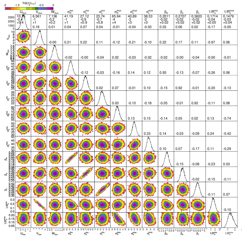
Figure 10.— Marginalized posterior distribution of model parameters.The numbers are the linear Pearson correlation coefficient. Shown is the case of Gaussian model for GCS data (column 1 of Table 7). Strong dependency can be seen between $\beta$ and $\sigma^{\rm thin}$ values. Additionally, $(R_{\sigma}^{\rm thin},V_{\odot})$, $(R_{\sigma}^{\rm thin},\sigma_{R}^{\rm thin})$, $(R_{\sigma}^{\rm thin},\beta_{R})$ and $(R_{\sigma}^{\rm thick},\sigma_{R}^{\rm thick})$ also show dependency.

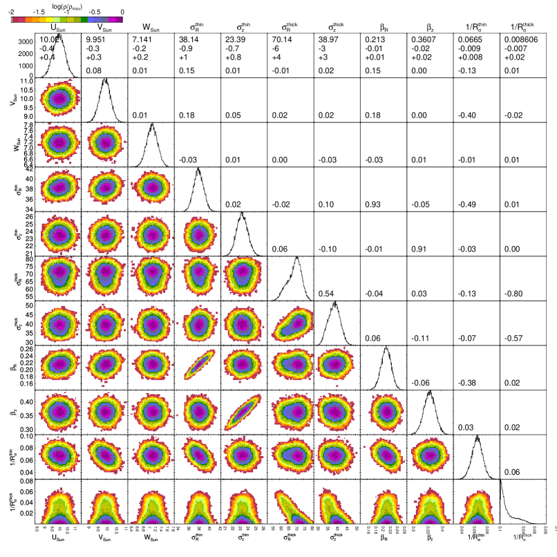
Figure 11.— Marginalized posterior distribution of model parameters.The numbers are the linear Pearson correlation coefficient. Shown is the case of Shu model for GCS data (column 1 of Table 7). Same dependencies as in LABEL:gcs_gauss can be seen. Dependency of $(R_{\sigma}^{\rm thin},V_{\odot})$ has got weaker while that of $(R_{\sigma}^{\rm thick},\sigma_{R}^{\rm thick})$ has become stronger.

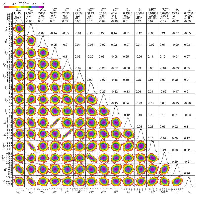
Figure 12.— Marginalized posterior distribution of model parameters.The numbers are the linear Pearson correlation coefficient. Shown is the case of Gaussian model for RAVE data (column 5 of Table 7). Strong dependency can be seen between $\beta$ and $\sigma^{\rm thin}$ values. Additionally, $(R_{\sigma}^{\rm thin},V_{\odot})$ and $(R_{\sigma}^{\rm thick},\sigma_{R}^{\rm thick})$ also show dependency. Finally, the $\Theta_{0}$ is anti-correlated to $U_{\odot}$ and $\alpha_{z}$ to $V_{\odot}$.

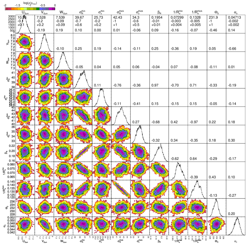
Figure 13.— Marginalized posterior distribution of model parameters.The numbers are the linear Pearson correlation coefficient. Shown is the case of Shu model for RAVE data (column 6 of Table 7). Strong dependency can be seen between $\beta$ and $\sigma^{\rm thin}$ values. Additionally, $(R_{\sigma}^{\rm thin},V_{\odot})$, $(R_{\sigma}^{\rm thin},\sigma_{R}^{\rm thin})$, $(R_{\sigma}^{\rm thin},\beta_{R})$ and $(R_{\sigma}^{\rm thick},\sigma_{R}^{\rm thick})$ also show dependency. Unlike GCS a dependency of $(\sigma_{R}^{\rm thin},\sigma_{R}^{\rm thick})$ and $(\beta_{z},\beta_{R})$ can be seen. Finally, the $\Theta_{0}$ is anti-correlated to $U_{\odot}$ and $\alpha_{z}$ to $V_{\odot}$.

References

- Abadi et al. (2003) Abadi, M. G., Navarro, J. F., Steinmetz, M., & Eke, V. R. 2003, ApJ, 591, 499
- Abazajian et al. (2009) Abazajian, K. N., Adelman-McCarthy, J. K., Agüeros, M. A., et al. 2009, ApJS, 182, 543
- Andrieu & Thoms (2008) Andrieu, C., & Thoms, J. 2008, Statistics and Computing, 18, 343
- Appourchaux et al. (2008) Appourchaux, T., Michel, E., Auvergne, M., et al. 2008, A&A, 488, 705
- Arce & Goodman (1999) Arce, H. G., & Goodman, A. A. 1999, ApJ, 512, L135
- Aumer & Binney (2009) Aumer, M., & Binney, J. J. 2009, MNRAS, 397, 1286
- Aumer & White (2013) Aumer, M., & White, S. D. M. 2013, MNRAS, 428, 1055
- Bahcall & Soneira (1980a) Bahcall, J. N., & Soneira, R. M. 1980a, ApJ, 238, L17
- Bahcall & Soneira (1980b) —. 1980b, ApJS, 44, 73
- Bahcall & Soneira (1984) —. 1984, ApJS, 55, 67
- Bensby et al. (2003) Bensby, T., Feltzing, S., & Lundström, I. 2003, A&A, 410, 527
- Bensby et al. (2005) Bensby, T., Feltzing, S., Lundström, I., & Ilyin, I. 2005, A&A, 433, 185
- Bertelli et al. (1994) Bertelli, G., Bressan, A., Chiosi, C., Fagotto, F., & Nasi, E. 1994, A&AS, 106, 275
- Bienayme et al. (1987) Bienayme, O., Robin, A. C., & Creze, M. 1987, A&A, 180, 94
- Binney (2010) Binney, J. 2010, MNRAS, 401, 2318
- Binney (2012a) —. 2012a, MNRAS, 426, 1324
- Binney (2012b) —. 2012b, MNRAS, 426, 1328
- Binney (2013) —. 2013, Dynamics of secular evolution (Cambridge University Press), 259
- Binney et al. (2000) Binney, J., Dehnen, W., & Bertelli, G. 2000, MNRAS, 318, 658
- Binney & Lacey (1988) Binney, J., & Lacey, C. 1988, MNRAS, 230, 597
- Binney & McMillan (2011) Binney, J., & McMillan, P. 2011, MNRAS, 413, 1889
- Binney & Tremaine (2008) Binney, J., & Tremaine, S. 2008, Galactic Dynamics: Second Edition (Princeton University Press)
- Binney et al. (2014) Binney, J., Burnett, B., Kordopatis, G., et al. 2014, MNRAS, doi:10.1093/mnras/stt2367
- Boeche et al. (2013) Boeche, C., Chiappini, C., Minchev, I., et al. 2013, A&A, 553, A19
- Bond et al. (2010) Bond, N. A., Ivezić, Ž., Sesar, B., et al. 2010, ApJ, 716, 1
- Bournaud et al. (2009) Bournaud, F., Elmegreen, B. G., & Martig, M. 2009, ApJ, 707, L1
- Bovy et al. (2012a) Bovy, J., Rix, H.-W., & Hogg, D. W. 2012a, ApJ, 751, 131
- Bovy et al. (2012b) Bovy, J., Rix, H.-W., Hogg, D. W., et al. 2012b, ApJ, 755, 115
- Bovy et al. (2012c) Bovy, J., Rix, H.-W., Liu, C., et al. 2012c, ApJ, 753, 148
- Bovy et al. (2012d) Bovy, J., Allende Prieto, C., Beers, T. C., et al. 2012d, ApJ, 759, 131
- Brook et al. (2004) Brook, C. B., Kawata, D., Gibson, B. K., & Freeman, K. C. 2004, ApJ, 612, 894
- Cambrésy et al. (2005) Cambrésy, L., Jarrett, T. H., & Beichman, C. A. 2005, A&A, 435, 131
- Carlberg & Sellwood (1985) Carlberg, R. G., & Sellwood, J. A. 1985, ApJ, 292, 79
- Casagrande et al. (2011) Casagrande, L., Schönrich, R., Asplund, M., et al. 2011, A&A, 530, A138
- Chaplin et al. (2010) Chaplin, W. J., Appourchaux, T., Elsworth, Y., et al. 2010, ApJ, 713, L169
- Chaplin et al. (2011) Chaplin, W. J., Kjeldsen, H., Christensen-Dalsgaard, J., et al. 2011, Science, 332, 213
- Chiba & Beers (2000) Chiba, M., & Beers, T. C. 2000, AJ, 119, 2843
- Dehnen & Binney (1998a) Dehnen, W., & Binney, J. 1998a, MNRAS, 294, 429
- Dehnen & Binney (1998b) Dehnen, W., & Binney, J. J. 1998b, MNRAS, 298, 387
- Delhaye (1965) Delhaye, J. 1965, in Galactic Structure, ed. A. Blaauw & M. Schmidt, 61
- Di Matteo et al. (2011) Di Matteo, P., Lehnert, M. D., Qu, Y., & van Driel, W. 2011, A&A, 525, L3
- Edvardsson et al. (1993) Edvardsson, B., Andersen, J., Gustafsson, B., et al. 1993, A&A, 275, 101
- Epchtein et al. (1999) Epchtein, N., Deul, E., Derriere, S., et al. 1999, A&A, 349, 236
- Forbes et al. (2012) Forbes, J., Krumholz, M., & Burkert, A. 2012, ApJ, 754, 48
- Freeman & Bland-Hawthorn (2008) Freeman, K., & Bland-Hawthorn, J. 2008, in Astronomical Society of the Pacific Conference Series, Vol. 399, Astronomical Society of the Pacific Conference Series, ed. T. Kodama, T. Yamada, & K. Aoki, 439–+
- Fuhrmann (1998) Fuhrmann, K. 1998, A&A, 338, 161
- Gelfand & Smith (1990) Gelfand, A. E., & Smith, A. F. 1990, Journal of the American statistical association, 85, 398
- Gelman et al. (1996) Gelman, A., Roberts, G., & Gilks, W. 1996, Bayesian statistics, 5, 599
- Gillessen et al. (2009) Gillessen, S., Eisenhauer, F., Trippe, S., et al. 2009, ApJ, 692, 1075
- Gilmore & Reid (1983) Gilmore, G., & Reid, N. 1983, MNRAS, 202, 1025
- Gilmore et al. (2012) Gilmore, G., Randich, S., Asplund, M., et al. 2012, The Messenger, 147, 25
- Girard et al. (2011) Girard, T. M., van Altena, W. F., Zacharias, N., et al. 2011, AJ, 142, 15
- Girardi et al. (2005) Girardi, L., Groenewegen, M. A. T., Hatziminaoglou, E., & da Costa, L. 2005, A&A, 436, 895
- Golubov et al. (2013) Golubov, O., Just, A., Bienaymé, O., et al. 2013, A&A, 557, A92
- Gomez et al. (1997) Gomez, A. E., Grenier, S., Udry, S., et al. 1997, in ESA Special Publication, Vol. 402, Hipparcos - Venice ’97, ed. R. M. Bonnet, E. Høg, P. L. Bernacca, L. Emiliani, A. Blaauw, C. Turon, J. Kovalevsky, L. Lindegren, H. Hassan, M. Bouffard, B. Strim, D. Heger, M. A. C. Perryman, & L. Woltjer, 621–624
- Górski et al. (2005) Górski, K. M., Hivon, E., Banday, A. J., et al. 2005, ApJ, 622, 759
- Hänninen & Flynn (2002) Hänninen, J., & Flynn, C. 2002, MNRAS, 337, 731
- Haywood et al. (1997a) Haywood, M., Robin, A. C., & Creze, M. 1997a, A&A, 320, 428
- Haywood et al. (1997b) —. 1997b, A&A, 320, 440
- Høg et al. (2000) Høg, E., Fabricius, C., Makarov, V. V., et al. 2000, A&A, 355, L27
- Holmberg et al. (2007) Holmberg, J., Nordström, B., & Andersen, J. 2007, A&A, 475, 519
- Holmberg et al. (2009) —. 2009, A&A, 501, 941
- Ida et al. (1993) Ida, S., Kokubo, E., & Makino, J. 1993, MNRAS, 263, 875
- Ivezić et al. (2008) Ivezić, Ž., Sesar, B., Jurić, M., et al. 2008, ApJ, 684, 287
- Jenkins (1992) Jenkins, A. 1992, MNRAS, 257, 620
- Jurić et al. (2008) Jurić, M., Ivezić, Ž., Brooks, A., et al. 2008, ApJ, 673, 864
- Just & Jahreiß (2010) Just, A., & Jahreiß, H. 2010, MNRAS, 402, 461
- Kazantzidis et al. (2008) Kazantzidis, S., Bullock, J. S., Zentner, A. R., Kravtsov, A. V., & Moustakas, L. A. 2008, ApJ, 688, 254
- Kazantzidis et al. (2009) Kazantzidis, S., Zentner, A. R., Kravtsov, A. V., Bullock, J. S., & Debattista, V. P. 2009, ApJ, 700, 1896
- Kordopatis et al. (2013) Kordopatis, G., Gilmore, G., Steinmetz, M., et al. 2013, AJ, 146, 134
- Lacey & Ostriker (1985) Lacey, C. G., & Ostriker, J. P. 1985, ApJ, 299, 633
- Law & Majewski (2010) Law, D. R., & Majewski, S. R. 2010, ApJ, 714, 229
- Lewis & Freeman (1989) Lewis, J. R., & Freeman, K. C. 1989, AJ, 97, 139
- Loebman et al. (2011) Loebman, S. R., Roškar, R., Debattista, V. P., et al. 2011, ApJ, 737, 8
- Marigo et al. (2008) Marigo, P., Girardi, L., Bressan, A., et al. 2008, A&A, 482, 883
- McMillan & Binney (2010) McMillan, P. J., & Binney, J. J. 2010, MNRAS, 402, 934
- Minchev et al. (2013) Minchev, I., Chiappini, C., & Martig, M. 2013, A&A, 558, A9
- Minchev & Famaey (2010) Minchev, I., & Famaey, B. 2010, ApJ, 722, 112
- Minchev & Quillen (2006) Minchev, I., & Quillen, A. C. 2006, MNRAS, 368, 623
- Nordström et al. (2004) Nordström, B., Mayor, M., Andersen, J., et al. 2004, A&A, 418, 989
- Ojha et al. (1996) Ojha, D. K., Bienayme, O., Robin, A. C., Creze, M., & Mohan, V. 1996, A&A, 311, 456
- Pasetto et al. (2012a) Pasetto, S., Grebel, E. K., Zwitter, T., et al. 2012a, A&A, 547, A70
- Pasetto et al. (2012b) —. 2012b, A&A, 547, A71
- Perryman et al. (1997) Perryman, M. A. C., Lindegren, L., Kovalevsky, J., et al. 1997, A&A, 323, L49
- Quillen & Garnett (2001) Quillen, A. C., & Garnett, D. R. 2001, in Astronomical Society of the Pacific Conference Series, Vol. 230, Galaxy Disks and Disk Galaxies, ed. J. G. Funes & E. M. Corsini, 87–88
- Quinn et al. (1993) Quinn, P. J., Hernquist, L., & Fullagar, D. P. 1993, ApJ, 403, 74
- Reid (1993) Reid, M. J. 1993, ARA&A, 31, 345
- Reid & Brunthaler (2004) Reid, M. J., & Brunthaler, A. 2004, ApJ, 616, 872
- Reid & Majewski (1993) Reid, N., & Majewski, S. R. 1993, ApJ, 409, 635
- Robin & Creze (1986) Robin, A., & Creze, M. 1986, A&A, 157, 71
- Robin et al. (2003) Robin, A. C., Reylé, C., Derrière, S., & Picaud, S. 2003, A&A, 409, 523
- Röser et al. (2008) Röser, S., Schilbach, E., Schwan, H., et al. 2008, A&A, 488, 401
- Roškar et al. (2010) Roškar, R., Debattista, V. P., Brooks, A. M., et al. 2010, MNRAS, 408, 783
- Sale (2012) Sale, S. E. 2012, MNRAS, 427, 2119
- Sales et al. (2012) Sales, L. V., Navarro, J. F., Theuns, T., et al. 2012, MNRAS, 423, 1544
- Schlegel et al. (1998) Schlegel, D. J., Finkbeiner, D. P., & Davis, M. 1998, ApJ, 500, 525
- Schönrich (2012) Schönrich, R. 2012, MNRAS, 427, 274
- Schönrich & Binney (2009a) Schönrich, R., & Binney, J. 2009a, MNRAS, 396, 203
- Schönrich & Binney (2009b) —. 2009b, MNRAS, 399, 1145
- Schönrich & Binney (2012) —. 2012, MNRAS, 419, 1546
- Schönrich et al. (2010) Schönrich, R., Binney, J., & Dehnen, W. 2010, MNRAS, 403, 1829
- Seabroke (2008) Seabroke, G. 2008, The Observatory, 128, 520
- Seabroke & Gilmore (2007) Seabroke, G. M., & Gilmore, G. 2007, MNRAS, 380, 1348
- Sellwood (2008) Sellwood, J. A. 2008, ASPCS, 396, 241
- Sellwood (2013) —. 2013, ApJ, 769, L24
- Sharma & Bland-Hawthorn (2013) Sharma, S., & Bland-Hawthorn, J. 2013, ApJ, 773, 183
- Sharma et al. (2011) Sharma, S., Bland-Hawthorn, J., Johnston, K. V., & Binney, J. 2011, ApJ, 730, 3
- Sharma et al. (2012) Sharma, S., Steinmetz, M., & Bland-Hawthorn, J. 2012, ApJ, 750, 107
- Shiidsuka & Ida (1999) Shiidsuka, K., & Ida, S. 1999, MNRAS, 307, 737
- Shu (1969) Shu, F. H. 1969, ApJ, 158, 505
- Siebert et al. (2008) Siebert, A., Bienaymé, O., Binney, J., et al. 2008, MNRAS, 391, 793
- Siebert et al. (2011) Siebert, A., Williams, M. E. K., Siviero, A., et al. 2011, AJ, 141, 187
- Skrutskie et al. (2006) Skrutskie, M. F., Cutri, R. M., Stiening, R., et al. 2006, AJ, 131, 1163
- Soubiran et al. (2003) Soubiran, C., Bienaymé, O., & Siebert, A. 2003, A&A, 398, 141
- Spitzer & Schwarzschild (1953) Spitzer, Jr., L., & Schwarzschild, M. 1953, ApJ, 118, 106
- Steinmetz et al. (2006) Steinmetz, M., Zwitter, T., Siebert, A., et al. 2006, AJ, 132, 1645
- Tanner & Wong (1987) Tanner, M. A., & Wong, W. H. 1987, Journal of the American statistical Association, 82, 528
- Tierney (1994) Tierney, L. 1994, the Annals of Statistics, 1701
- van der Kruit (1988) van der Kruit, P. C. 1988, A&A, 192, 117
- van der Kruit & Freeman (2011) van der Kruit, P. C., & Freeman, K. C. 2011, ARA&A, 49, 301
- van der Kruit & Searle (1982) van der Kruit, P. C., & Searle, L. 1982, A&A, 110, 61
- Villalobos & Helmi (2008) Villalobos, Á., & Helmi, A. 2008, MNRAS, 391, 1806
- Williams et al. (2013) Williams, M. E. K., Steinmetz, M., Binney, J., et al. 2013, MNRAS, 436, 101
- Yanny et al. (2009) Yanny, B., Rockosi, C., Newberg, H. J., et al. 2009, AJ, 137, 4377
- Yoachim & Dalcanton (2006) Yoachim, P., & Dalcanton, J. J. 2006, AJ, 131, 226
- Zacharias et al. (2004) Zacharias, N., Urban, S. E., Zacharias, M. I., et al. 2004, AJ, 127, 3043
- Zacharias et al. (2010) Zacharias, N., Finch, C., Girard, T., et al. 2010, AJ, 139, 2184
- Zwitter et al. (2008) Zwitter, T., Siebert, A., Munari, U., et al. 2008, AJ, 136, 421