Relativistic redshifts in quasar broad lines

Abstract

The broad emission lines commonly seen in quasar spectra have velocity widths of a few per cent of the speed of light, so special- and general-relativistic effects have a significant influence on the line profile. We have determined the redshift of the broad H$\beta$ line in the quasar rest frame (determined from the core component of the [O iii] line) for over 20,000 quasars from the Sloan Digital Sky Survey DR7 quasar catalog. The mean redshift as a function of line width is approximately consistent with the relativistic redshift that is expected if the line originates in a randomly oriented Keplerian disk that is obscured when the inclination of the disk to the line of sight exceeds $\sim 30^{\circ}$–$45^{\circ}$, consistent with simple AGN unification schemes. This result also implies that the net line-of-sight inflow/outflow velocities in the broad-line region are much less than the Keplerian velocity when averaged over a large sample of quasars with a given line width.

1 Introduction

Quasars and other active galactic nuclei (AGN) are accreting supermassive black holes (BHs). Among the prominent features in their spectra are broad emission lines, which are thought to arise from a broad line region (BLR) close to the BH in which gas has been photoionized by the quasar continuum emission. The line widths are believed to arise from Doppler shifts, typically thousands of $\,{\rm km\ s}^{-1}$, due to orbital motion of the gas in the gravitational field of the BH, and/or large-scale inflows or outflows. This general picture is supported by measurements of the BLR size through reverberation mapping (RM; see, e.g., Peterson et al., 2004; Bentz et al., 2009). On larger spatial scales, where the dynamical influence of the BH is less important, there is a narrow line region (NLR), where the gas emits with typical line widths of hundreds of $\,{\rm km\ s}^{-1}$. Unification schemes (Antonucci, 1993; Urry & Padovani, 1995) seek to explain the diverse properties of AGN as a result of viewing a single generic structure with different viewing angles. The typical unification scheme includes, in order of increasing size, the central BH, a surrounding accretion disk, the BLR, a thick dusty torus aligned with the disk that obscures the accretion disk and the BLR when viewed at high inclinations, and the NLR. Whether or not the accretion disk and BLR are obscured produces the dichotomy between broad-line (Type 1) and narrow-line (Type 2) AGN.

The proximity of the BLR to the BH allows us to look for special- and general-relativistic effects on the observed broad lines, and thereby to test relativity or, more plausibly, to constrain the structure of the BLR assuming relativity is correct. There have been several attempts in the past to detect relativistic effects in broad quasar lines (e.g., Zheng & Sulentic, 1990; McIntosh et al., 1999; Kollatschny, 2003), but these studies mostly lacked a general treatment that included all relativistic effects, and were limited to small samples of objects where the relativistic effects are easily swamped by astrophysical effects such as object-to-object variations in the line profiles. A complementary approach has been to model the BLR as a rotating, axisymmetric disk (“disk-emitter” models), include relativistic effects rigorously, at least to $\mbox{O}(v^{2}/c^{2})$ (Chen et al., 1989; Eracleous et al., 1995), and fit these models to the small fraction of quasars that show double-peaked broad line profiles, which are likely to be produced by inclined disks in which the emission is dominated by a small range of radii (e.g., Eracleous & Halpern, 2003; Strateva et al., 2003). However, disk-emitter models of the BLR have yet to be tested against the general quasar population. A robust detection of relativistic effects in quasar broad lines is therefore still absent.

In this work we present a simple treatment of relativistic effects on the spectrum of the BLR, and use kinematic properties of the broad line (centroid velocity shift and line width) to constrain the geometry of the BLR, assuming that the gas is in a steady state and that its kinematics are determined by the gravitational field of the central BH (“virialized”). We use the large spectroscopic quasar sample from the Sloan Digital Sky Survey (SDSS, Schneider et al., 2010), which allows us to average out object-to-object measurement errors and variations in line profile.

2 Models of the kinematics of the broad-line region

First, we examine simple models of the structure of the BLR to illustrate how relativistic effects can discriminate between models. In all of our models we assume that the BLR gas is in a steady-state dynamical equilibrium, orbiting under the influence of the gravitational field of the central BH (“virial equilibrium”).

Let $\lambda$ be the observed wavelength of the line photon in the rest frame of the central BH and $\lambda_{0}$ the rest wavelength of the line transition. The corresponding photon energy is $E=E_{0}(\lambda_{0}/\lambda)$ with $E_{0}=hc/\lambda_{0}$ and the redshift is $z=\lambda/\lambda_{0}-1$. The redshift of the rest frame of the BH is assumed to be the same as the redshift of the narrow-line region of the quasar; thus $z$ is related to the observed redshift of the broad and narrow lines by $1+z=(1+z_{\rm blr})/(1+z_{\rm nlr})$.

For each model we determine the relation between the mean redshift $\langle z\rangle$ and the rms redshift $\langle z^{2}\rangle^{1/2}$. In general $\mbox{O}(\langle z\rangle)=\mbox{O}(\langle z^{2}\rangle)=\mbox{O}(v^{2}/c^{2})$ where $v$ is a typical velocity in the BLR.

One complication in comparing with the extensive earlier work on this subject is that some authors measure the photon-weighted mean while others measure the energy-weighted mean. Let $f_{\lambda}d\lambda$ be the energy flux received at the detector in the wavelength range $(\lambda,\lambda+d\lambda)$. We define the moment

$$J_{n}=\int d\lambda\,f_{\lambda}(\lambda/\lambda_{0})^{n}.$$ (1)

Then the photon- and energy-weighted mean redshifts are given by

$$\langle z\rangle_{N}=\langle\lambda/\lambda_{0}\rangle_{N}-1\equiv\frac{J_{2}}{J_{1}}-1,\quad\langle z\rangle_{E}=\langle\lambda/\lambda_{0}\rangle_{E}-1\equiv\frac{J_{1}}{J_{0}}-1.$$ (2)

Instead of the wavelength shift some authors use the frequency shift,

$$\langle\nu/\nu_{0}\rangle_{N}\equiv\frac{J_{0}}{J_{1}},\quad\langle\nu/\nu_{0}\rangle_{E}\equiv\frac{J_{-1}}{J_{0}}.$$ (3)

In general all four of these quantities will be different.

Although these distinctions are important in measuring the mean wavelength or frequency shift, we need make no such distinction between the second moments $\langle(\lambda/\lambda_{0}-1)^{2}\rangle$ and $\langle(\nu/\nu_{0}-1)^{2}\rangle$ or between photon- and energy-weighted second moments, since these are already $\mbox{O}(v^{2}/c^{2})$. In particular we can write $\langle(\lambda/\lambda_{0}-1)^{2}\rangle=\langle(\nu/\nu_{0}-1)^{2}\rangle=\langle z^{2}\rangle$ to $\mbox{O}(v^{2}/c^{2})$ for both photon-weighted and energy-weighted averages and all of these quantities are equal to $\sigma^{2}/c^{2}$ where $\sigma$ is the line-of-sight velocity dispersion or the standard deviation of the spectral line.

2.1 Relativistic kinematics

The following derivations and formulas are well-known (e.g., Rybicki & Lightman, 1979), but we collect them here for reference.

We denote the quasar rest frame by spacetime coordinates $(t,{\bf x})$. We assume that this is the rest frame of the quasar’s central BH and of the narrow-line region. We denote the rest frame of an emitting mass element of the BLR by coordinates $(t_{0},{\bf x}_{0})$ and for simplicity we assume that $(t_{0},{\bf x}_{0})={\bf 0}$ when $(t,{\bf x})={\bf 0}$. If the velocity of the emitting element relative to the quasar rest frame is ${\bf v}$, then

$${\bf x}_{0}={\bf x}-\gamma{\bf v}t+(\gamma-1)\frac{{\bf x}\cdot{\bf v}}{v^{2}}{\bf v},\quad \quad{\bf x}={\bf x}_{0}+\gamma{\bf v}t_{0}+(\gamma-1)\frac{{\bf x}_{0}\cdot{\bf v}}{v^{2}}{\bf v},$$

$$t_{0}=\gamma(t-{\bf v}\cdot{\bf x}),\quad \quad t=\gamma(t_{0}+{\bf v}\cdot{\bf x}_{0})$$ (4)

where $\gamma\equiv(1-v^{2})^{-1/2}$ and in this subsection we have set the speed of light $c$ to unity for brevity. Similarly, the momentum and energy in the two frames are related by

$${\bf p}_{0}={\bf p}-\gamma{\bf v}E+(\gamma-1)\frac{{\bf p}\cdot{\bf v}}{v^{2}}{\bf v},\quad E_{0}=\gamma(E-{\bf v}\cdot{\bf p}).$$ (5)

For photons $E=p$, $E_{0}=p_{0}$, so if we write ${\bf p}=E\hat{\bf n}$ we have

$$E_{0}=\gamma E(1-\hat{\bf n}\cdot{\bf v}),\quad\hat{\bf n}_{0}=\frac{\hat{\bf n}-\gamma{\bf v}+(\gamma-1)(\hat{\bf n}\cdot{\bf v})\,{\bf v}/v^{2}}{\gamma(1-\hat{\bf n}\cdot{\bf v})}.$$ (6)

If the mass element emits photons with wavelength $\lambda_{0}$ in its rest frame, the wavelength in the quasar rest frame is

$$\frac{\lambda}{\lambda_{0}}=\frac{E_{0}}{E}=\gamma(1-\hat{\bf n}\cdot{\bf v}).$$ (7)

Let $\mu=\hat{\bf n}\cdot{\bf v}/v$ be the cosine of the angle between the path of the emitted photon and the velocity vector in the quasar rest frame, with a similar definition for $\mu_{0}$ in the rest frame of the emitter. Then from equations (6)

$$\mu_{0}=\frac{\mu-v}{1-\mu v},\quad\mu=\frac{\mu_{0}+v}{1+\mu_{0}v}.$$ (8)

Thus the elements of solid angle in the two frames are related by

$$d\Omega_{0}=d\Omega\frac{d\mu_{0}}{d\mu}=\frac{d\Omega}{\gamma^{2}(1-\mu v)^{2}}.$$ (9)

If photons are emitted at a rate $d\dot{N}_{e0}(\Omega_{0})$ into a small element of solid angle $d\Omega_{0}$ in the rest frame of the emitting material, then they are received at a rate $d\dot{N}_{r}(\Omega)dt_{r}=d\dot{N}_{e0}(\Omega_{0})dt_{e0}$ within a small element of solid angle $d\Omega$; here $t_{e0}$ is the emission time in the rest frame of the emitter and $t_{r}$ is the time when they are received in the frame of the observer. If the observer is at position ${\bf X}=\mbox{const}$ then $t_{r}=t_{e}+|{\bf X}-{\bf x}_{e}|$. The emitting element has ${\bf x}_{0}=\mbox{const}$ so equations (4) give $d{\bf x}_{e}=\gamma{\bf v}dt_{e0}$ and $dt_{e}=\gamma dt_{e0}$; then

$$dt_{r}=\gamma dt_{e0}-\frac{({\bf X}-{\bf x}_{e})\cdot d{\bf x}_{e}}{|{\bf X}-{\bf x}_{e}|}=\gamma(1-\mu v)dt_{e0}+\mbox{O}(X^{-1}).$$ (10)

Since $X$ is astronomically large we can drop the terms proportional to $1/X$. Then

$$\frac{d\dot{N}_{r}}{d\Omega}=\frac{1}{\gamma^{3}(1-\mu v)^{3}}\frac{d\dot{N}_{e0}}{d\Omega_{0}};$$ (11)

the subscript “$r$” indicates that this is the rate at which photons are received by the observer.

At this point a subtle correction is required. Let $dN_{\rm EM}/d\Omega$ be the total number of photons that are in transit from the emitter to the observer, with momenta pointing into the solid angle $d\Omega$. In the rest frame of the observer $dN_{\rm EM}/d\Omega=(d\dot{N}_{r}/d\Omega)|{\bf X}-{\bf x}_{e}|$ (recall that $c=1$). The rate of change of the photon number is $d\dot{N}_{\rm EM}/d\Omega=-\mu v(d\dot{N}_{r}/d\Omega)+\mbox{O}(X^{-1})$. If the rate of emission of photons is $d\dot{N}_{e}/d\Omega$ then by continuity $d\dot{N}_{\rm EM}/d\Omega=d\dot{N}_{e}/d\Omega-d\dot{N}_{r}/d\Omega$ so $d\dot{N}_{e}/d\Omega=(1-\mu v)d\dot{N}_{r}/d\Omega$. We may then ask, is the shape of the observed spectral line determined by $d\dot{N}_{e}/d\Omega$ or $d\dot{N}_{r}/d\Omega$, which differ because of the changing number of photons in transit. In a steady-state system, with emitting elements traveling both towards and away from the observer, the total number of photons in transit should be constant after averaging over all the emitting elements. This means that the average should be taken over the rate at which photons are emitted rather than the rate at which they are detected; that is, we should work with

$$\frac{d\dot{N}_{e}}{d\Omega}=\frac{1}{\gamma^{3}(1-\mu v)^{2}}\frac{d\dot{N}_{e0}}{d\Omega_{0}}.$$ (12)

Kaiser (2013) calls this the “light cone effect” and argues as follows. We see emitting bodies on the past light cone. Their separation $dx_{\rm LC}$ along the line of sight on the light cone is related to their separation at fixed time $dx$ by $dx_{\rm LC}=dx/(1-\mu v)$ so their observed density is larger than the density at fixed time by a factor $dx/dx_{\rm LC}=1-\mu v$. In other words we see more mass elements moving away from us than toward us. To correct for this effect in a steady-state system, we must multiply $d\dot{N}_{r}/d\Omega$ by $1-\mu v$, which converts equation (11) to equation (12).

If the photons are emitted in a spectral line with energy $E_{0}$ then the rate of energy emission in the observer frame is

$$\frac{dP_{e}}{d\Omega}=E\frac{d\dot{N}_{e}}{d\Omega}=\frac{E}{\gamma^{3}(1-\mu v)^{2}}\frac{d\dot{N}_{e0}}{d\Omega_{0}}\quad\mbox{where}\quad E=\frac{E_{0}}{\gamma(1-\mu v)}.$$ (13)

This can be rewritten in terms of the energy flux per unit wavelength at the detector,

$$f_{\lambda}=\frac{1}{X^{2}}\frac{dP_{e}}{d\Omega}\delta[\lambda-\lambda_{0}\gamma(1-\mu v)].$$ (14)

If the emitting region is optically thin, and composed of a large number of discrete clouds that radiate isotropically, then $d\dot{N}_{e0}/d\Omega_{0}$ is independent of direction and the integrals (1) become

$$J_{n}=\mbox{const}\times\langle\gamma^{n-4}(1-\mu v)^{n-3}\rangle,$$ (15)

where the brackets $\langle\cdot\rangle$ denote a luminosity-weighted average over the clouds. To O$(v^{2})$,

$$J_{n}=\mbox{const}\times[1+{\textstyle{1\over 2}}(n-4)\langle v^{2}\rangle+{\textstyle{1\over 2}}(n-3)(n-4)\langle\mu^{2}v^{2}\rangle],$$ (16)

in which we have assumed that $\langle\mu v\rangle=0$ as required for a steady state. Then, for example, equation (2) yields an energy-weighted mean redshift $\langle z\rangle_{E,\rm SR}={\textstyle{1\over 2}}\langle v^{2}\rangle-3\langle\mu^{2}v^{2}\rangle$ to $\mbox{O}(v^{2})$. The subscript “SR” is a reminder that this calculation accounts only for special-relativistic effects. In addition there is a gravitational redshift equal to $-\langle\Phi\rangle$ where $\Phi$ is the gravitational potential. For a point-mass potential like that of a BH, the virial theorem implies that $\langle\Phi\rangle+\langle v^{2}\rangle=0$ in a steady state; this is a classical result but relativistic corrections are of higher order than we are considering. Adding this correction yields $\langle z\rangle=\langle z\rangle_{\rm SR}+\langle v^{2}\rangle$, $\langle\nu/\nu_{0}\rangle=\langle\nu/\nu_{0}\rangle_{\rm SR}-\langle v^{2}\rangle$, both to $\mbox{O}(v^{2})$. Thus the photon- and energy-weighted mean redshifts are

$$\langle z\rangle_{N}={\textstyle\frac{3}{2}}\langle v^{2}\rangle-2\langle\mu^{2}v^{2}\rangle,\quad\langle z\rangle_{E}={\textstyle\frac{3}{2}}\langle v^{2}\rangle-3\langle\mu^{2}v^{2}\rangle.$$ (17)

The analogous equations (3) for the frequency shift are

$$\langle\nu/\nu_{0}\rangle_{N}=1-{\textstyle\frac{3}{2}}\langle v^{2}\rangle+3\langle\mu^{2}v^{2}\rangle,\quad\langle\nu/\nu_{0}\rangle_{E}=1-{\textstyle\frac{3}{2}}\langle v^{2}\rangle+4\langle\mu^{2}v^{2}\rangle.$$ (18)

For a spherically symmetric distribution of clouds $\langle\mu^{2}\rangle=\frac{1}{3}$ and we have

$$\langle z\rangle_{N}={\textstyle\frac{5}{6}}\langle v^{2}\rangle,\quad\langle z\rangle_{E}={\textstyle\frac{1}{2}}\langle v^{2}\rangle,\quad\langle\nu/\nu_{0}\rangle_{N}=1-{\textstyle\frac{1}{2}}\langle v^{2}\rangle,\quad\langle\nu/\nu_{0}\rangle_{E}=1-{\textstyle\frac{1}{6}}\langle v^{2}\rangle.$$ (19)

For comparison, Kaiser (2013) finds (at the end of his §3) $\langle\nu/\nu_{0}\rangle_{N,\rm SR}=1+{\textstyle{1\over 2}}\langle v^{2}\rangle$ which after adding the gravitational redshift yields $\langle\nu/\nu_{0}\rangle_{N}=1-{\textstyle{1\over 2}}\langle v^{2}\rangle$, consistent with our result.

If the clouds are in an optically thin disk, with normal inclined by $I$ to the line of sight, then $\langle\mu^{2}\rangle={\textstyle{1\over 2}}\sin^{2}I$ so

$$\langle z\rangle_{N}=\langle v^{2}\rangle({\textstyle\frac{3}{2}}-\sin^{2}I),\quad\langle z\rangle_{E}={\textstyle\frac{3}{2}}\langle v^{2}\rangle\cos^{2}I,$$

$$\langle\nu/\nu_{0}\rangle_{N}=1-{\textstyle\frac{3}{2}}\langle v^{2}\rangle\cos^{2}I,\quad\langle\nu/\nu_{0}\rangle_{E}=1+\langle v^{2}\rangle(2\sin^{2}I-1).$$ (20)

If the emitting material is an optically thick disk, $d\dot{N}_{e0}/d\Omega_{0}$ is proportional to $\cos\theta_{0}$ where $\theta_{0}$ is the angle between the disk normal $\hat{\bf z}$ and the photon momentum in the rest frame of the emitting material. Thus $\cos\theta_{0}=\hat{\bf z}\cdot\hat{\bf n}_{0}$ and observing that $\hat{\bf n}\cdot{\bf v}=0$ equation (6) yields

$$\cos\theta_{0}=\frac{\cos\theta}{\gamma(1-\mu v)},$$ (21)

where $\theta=I$ is the angle between the disk normal and the line of sight in the observer’s frame. The analog of equations (15) and (16) are then

$$J_{n}=\mbox{const}\times\langle\gamma^{n-5}(1-\mu v)^{n-4}\rangle=\mbox{const}\times[1+{\textstyle{1\over 2}}(n-5)\langle v^{2}\rangle+{\textstyle{1\over 2}}(n-4)(n-5)\langle\mu^{2}v^{2}\rangle].$$ (22)

Including gravitational redshift, the mean redshifts and frequency shifts are

$$\langle z\rangle_{N}={\textstyle\frac{3}{2}}\langle v^{2}\rangle\cos^{2}I,\quad\langle z\rangle_{E}=\langle v^{2}\rangle({\textstyle\frac{3}{2}}-2\sin^{2}I),$$

$$\langle\nu/\nu_{0}\rangle_{N}=1+\langle v^{2}\rangle(2\sin^{2}I-{\textstyle\frac{3}{2}}),\quad\langle\nu/\nu_{0}\rangle_{E}=1+\langle v^{2}\rangle({\textstyle\frac{5}{2}}\sin^{2}I-{\textstyle\frac{3}{2}}).$$ (23)

For the most part, these derivations are not new. The expressions for $\langle z\rangle_{E}$ and $\langle\nu/\nu_{0}\rangle_{E}$ are the same as equations (12) and (11) of Gerbal & Pelat (1981). Chen et al. (1989) derive an expression for the line profile $f_{\lambda}$ expected from an accretion disk; their derivation correctly captures all of the relativistic effects considered here. In addition, Chen et al. include the effects of gravitational lensing by the BH and calculate the shape of the line profile, not just its first moment. Lensing can affect the line profile but to the order we are considering its effects are symmetric in $z$ and so do not affect the first moment.

A complete description of relativistic effects in the spectra of optically thick disks is given by Cunningham (1975).

2.2 Spherical models

A simple model for the BLR consists of a large number of clouds, distributed in a sphere, moving under the influence of the gravity of the central BH, and in virial equilibrium. The density of clouds is sufficiently small that the BLR is optically thin. The line-of-sight velocity dispersion is related to the mean-square velocity by $\sigma^{2}=\frac{1}{3}\langle v^{2}\rangle$, and the mean redshift is given by equation (19),

$$\langle zc\rangle_{E}={\textstyle{1\over 2}}\langle v^{2}/c\rangle={\textstyle\frac{3}{2}}\sigma^{2}/c$$ (24)

where here and henceforth we restore factors of $c$ to the formulas. This result is independent of the shape of the velocity ellipsoid in the phase-space distribution of the clouds.

Since $\sigma/c$ is typically $\lesssim 0.03$ for our sample, the mean redshift $\langle zc\rangle$ is expected to be much less than the line width $\sigma$. Thus, while the rms width can be determined fairly reliably for a single quasar, the expected mean redshift cannot. Therefore we must average over many quasars. Let $\langle\cdot\rangle_{\sigma}$ denote the average over all quasars in our sample with rms width in a small range around $\sigma$, with equal weight given to each quasar. Then in spherical models

$$\llangle zc\rrangle_{E,\sigma}={\textstyle\frac{3}{2}}\sigma^{2}/c.$$ (25)

2.3 Disk models

The notion of a disk-like BLR is not new in the literature. Early evidence came from observations of radio-loud quasars, where the orientation of the accretion disk can be inferred from the resolved radio jet morphology, and the observed correlation between the width of the broad H$\beta$ line and the jet orientation can be accounted for if the BLR is a disk whose symmetry axis is aligned with the radio axis (e.g., Wills & Browne, 1986; Runnoe et al., 2013). A second argument for a disk-like BLR comes from the success of disk-emitter models in explaining double-peaked broad line profiles in some quasars (Chen et al., 1989; Eracleous et al., 1995). Dynamical modeling of RM data sets also favors a disk geometry in several local broad-line AGN (e.g., Pancoast et al., 2013).

A BLR disk with a small radial extent and moderate inclination should lead to a double-peaked broad line profile (e.g., Dumont & Collin-Souffrin, 1990; Eracleous, 1999). However, only about a few percent of BLRs in the general quasar population exhibit double-peaked lines (e.g., Strateva et al., 2003; Shen et al., 2011), which suggests that a wide range of radii in the disk contributes significantly to the observed emission. The derivations in this paper use angle brackets $\langle\cdot\rangle$ to denote luminosity-weighted averages over the spatial extent of the BLR and are equally valid whatever the range of radii in the BLR may be.

We assume that the BLR is a flat disk whose normal is inclined by an angle $I$ to the line of sight, in which the emitting material travels on circular orbits uniformly distributed in azimuth. The velocity $v$ is then the circular speed at a given radius. If the disk consists of an optically thin collection of emitting elements, we may use equation (20):

$$\langle zc\rangle_{E}={\textstyle\frac{3}{2}}\cos^{2}I\langle v^{2}/c\rangle,\quad\sigma^{2}={\textstyle{1\over 2}}\sin^{2}I\langle v^{2}\rangle.$$ (26)

If the disk is optically thick, as one would expect for a standard Shakura–Sunyaev accretion disk, then from equation (23):

$$\langle zc\rangle_{E}=({\textstyle\frac{3}{2}}-2\sin^{2}I)\langle v^{2}/c\rangle,\quad\sigma^{2}={\textstyle{1\over 2}}\sin^{2}I\langle v^{2}\rangle.$$ (27)

More generally, the emitting material in the disk would also have a dispersion in velocities. In an optically thin disk of discrete clouds, the dispersion arises from epicyclic motion and the radial, azimuthal, and normal dispersions $s_{R}$, $s_{\phi}$, $s_{z}$ can all be different (e.g., Binney & Tremaine, 2008). We write $s_{\phi}=f_{\phi}s_{R}$ and $s_{z}=f_{z}s_{R}$. Then the generalization of equations (26) is

$$\langle zc\rangle_{E} ={\textstyle\frac{3}{2}}\cos^{2}I\langle v^{2}/c\rangle+{\textstyle\frac{3}{2}}[(1+f_{\phi}^{2})\cos^{2}I+f_{z}^{2}(1-2\cos^{2}I)]s_{R}^{2}/c,$$

$$\sigma^{2} ={\textstyle{1\over 2}}\sin^{2}I\langle v^{2}\rangle+{\textstyle{1\over 2}}[(1+f_{\phi}^{2})\sin^{2}I+2f_{z}^{2}\cos^{2}I]s_{R}^{2}.$$ (28)

Note that this expression assumes that the dispersion makes a dynamical contribution to the virial theorem, that is, that $\langle\Phi+v^{2}+(1+f_{\phi}^{2}+f_{z}^{2})s_{R}^{2}\rangle=0$. For Keplerian potentials $f_{\phi}={\textstyle{1\over 2}}$; $f_{z}$ depends on the details of the disk dynamics but is typically also $\simeq 0.5$.

In an optically thick disk the dispersion would most likely arise from turbulence. If the turbulence is isotropic and the rms turbulent velocity along any one direction is $s$ then the generalization of (27) is

$$\langle zc\rangle_{E}=({\textstyle\frac{3}{2}}-2\sin^{2}I)\langle v^{2}/c\rangle+{\textstyle{1\over 2}}s^{2}/c,\quad\sigma^{2}={\textstyle{1\over 2}}\sin^{2}I\langle v^{2}\rangle+s^{2}.$$ (29)

This assumes that the dispersion makes a dynamical contribution to the virial theorem, $\langle\Phi+v^{2}+3s^{2}\rangle=0$. Of course the assumption that the turbulence is isotropic is questionable: for example if the turbulence is due to the magnetorotational instability it is likely anisotropic.

To proceed further we need to estimate the distribution of $\langle v^{2}\rangle$ for the quasars in our sample. We first give the derivation for optically thick disks (eq. 29). Let $u\equiv\langle v^{2}\rangle^{1/2}$ and $y=\langle zc\rangle_{E}$. Let the probability that a quasar in the sample lies in a small interval of $u$ and of inclination $I$ be $P(u)Q(\nu)dud\nu$ where $\nu=\cos I$, that is, we assume that the distribution in inclination and mean-square velocity is separable, as required in the simplest unification models. Then the joint probability distribution in rms line width $\sigma$ and flux-weighted mean redshift $\langle zc\rangle_{E}=y$ is

$$p(y,\sigma)=2\sigma\int\!dud\nu\,P(u)Q(\nu)\delta[y+({\textstyle\frac{1}{2}}-2\nu^{2})u^{2}/c-{\textstyle{1\over 2}}s^{2}/c]\delta[\sigma^{2}-{\textstyle{1\over 2}}u^{2}(1-\nu^{2})-s^{2}].$$ (30)

The probability distribution in rms line width is

$$p(\sigma)=\int p(y,\sigma)dy=2\sigma\int dud\nu\,P(u)Q(\nu)\delta[\sigma^{2}-{\textstyle{1\over 2}}u^{2}(1-\nu^{2})-s^{2}]$$ (31)

and the mean redshift of quasars at a given line width is

$$\llangle zc\rrangle_{E,\sigma} =\frac{\int p(y,\sigma)y\,dy}{\int p(y,\sigma)\,dy}$$

$$=\frac{\int dud\nu P(u)Q(\nu)[(2\nu^{2}-{\textstyle\frac{1}{2}})u^{2}+{\textstyle{1\over 2}}s^{2}]\delta[\sigma^{2}-{\textstyle{1\over 2}}u^{2}(1-\nu^{2})-s^{2}]}{c\int dud\nu P(u)Q(\nu)\delta[\sigma^{2}-{\textstyle{1\over 2}}u^{2}(1-\nu^{2})-s^{2}]}$$

$$=\frac{\displaystyle\int\frac{\displaystyle du\,P(u)Q(\sqrt{1+2(s^{2}-\sigma^{2})/u^{2}})}{u\sqrt{u^{2}+2s^{2}-2\sigma^{2}}}({\textstyle\frac{3}{2}}u^{2}+{\textstyle\frac{9}{2}}s^{2}-4\sigma^{2})}{\displaystyle c\int\frac{\displaystyle du\,P(u)Q(\sqrt{1+2(s^{2}-\sigma^{2})/u^{2}})}{u\sqrt{u^{2}+2s^{2}-2\sigma^{2}}}}.$$ (32)

The data are not sufficient to determine the functions $P(u)$ and $Q(I)$ directly. Instead we shall assume a simple model for $Q(I)$, motivated by the unification model: the disks are oriented isotropically, except that disks with inclination exceeding some opening angle $I_{\rm max}$ are obscured (Type 2 quasars) and thus do not appear in the sample (this model assumes that the BLR disk and the obscuring torus are coplanar). Then

$$Q(\nu)=\frac{1}{1-\cos I_{\rm max}},\qquad\cos I_{\rm max}\leq\nu\leq 1,$$ (33)

and zero otherwise. Then the distribution of line widths is

$$p(\sigma)=\frac{2\sigma}{1-\cos I_{\rm max}}\int_{u_{\rm min}}^{\infty}\frac{du\,P(u)}{u\sqrt{u^{2}+2s^{2}-2\sigma^{2}}},\qquad u_{\rm min}\equiv\frac{\sqrt{2(\sigma^{2}-s^{2})}}{\sin I_{\rm max}}$$ (34)

for $\sigma\geq s$, and zero otherwise. For given values of the disk dispersion $s$ and the maximum inclination $I_{\rm max}$, this equation can be solved for $P(u)$ given the known distribution of line widths $\sigma$ in our sample. Once this is done, the mean redshift as a function of line width is given by

$$\llangle zc\rrangle_{E,\sigma}=\frac{\displaystyle\int_{u_{\rm min}}^{\infty}\frac{\displaystyle du\,P(u)({\textstyle\frac{3}{2}}u^{2}+{\textstyle\frac{9}{2}}s^{2}-4\sigma^{2})}{\displaystyle u\sqrt{u^{2}+2s^{2}-2\sigma^{2}}}}{{\displaystyle c\int_{u_{\rm min}}^{\infty}}\,\frac{\displaystyle du\,P(u)}{\displaystyle u\sqrt{u^{2}+2s^{2}-2\sigma^{2}}}}.$$ (35)

The derivation for optically thin disks is similar. The analog to equation (34) is

$$p(\sigma) =\frac{2\sigma}{1-\cos I_{\rm max}}\int_{u_{\rm min}}^{\infty}\frac{du\,P(u)}{\sqrt{[u^{2}+(1+f_{\phi}^{2}-2f_{z}^{2})s_{R}^{2}][u^{2}-2\sigma^{2}+(1+f_{\phi}^{2})s_{R}^{2}]}},$$

$$u_{\rm min} \equiv\frac{\sqrt{2\sigma^{2}-[(1+f_{\phi}^{2})\sin^{2}I_{\rm max}+2f_{z}^{2}\cos^{2}I_{\rm max}]s_{R}^{2})}}{\sin I_{\rm max}}$$ (36)

and the analog to (35) is

$$\llangle zc\rrangle_{E,\sigma}=\frac{\displaystyle 3\int_{u_{\rm min}}^{\infty}\frac{du\,P(u)[u^{2}-2\sigma^{2}+(1+f_{\phi}^{2}+f_{z}^{2})s_{R}^{2}]}{\sqrt{[u^{2}+(1+f_{\phi}^{2}-2f_{z}^{2})s_{R}^{2}][u^{2}-2\sigma^{2}+(1+f_{\phi}^{2})s_{R}^{2}]}}}{\displaystyle 2c\int_{u_{\rm min}}^{\infty}\frac{du\,P(u)}{\sqrt{[u^{2}+(1+f_{\phi}^{2}-2f_{z}^{2})s_{R}^{2}][u^{2}-2\sigma^{2}+(1+f_{\phi}^{2})s_{R}^{2}]}}}.$$ (37)

3 The quasar sample

Our sample is drawn from the value-added Sloan Digital Sky Survey (SDSS) Data Release 7 (DR7) quasar catalog (Schneider et al., 2010; Shen et al., 2011). The parent quasar sample contains 105,783 quasars brighter than $M_{i}=-22.0$ that have at least one broad emission line with full-width at half-maximum (FWHM) larger than $1000\,{\rm km\ s}^{-1}$. The SDSS spectra used in this study are stored in vacuum wavelength, with a pixel scale of $10^{-4}$ in log₁₀-wavelength, which corresponds to $69\,{\rm km\ s}^{-1}$. The spectral resolution is $R\simeq 2000$. We only keep objects for which the SDSS spectrum covers the H$\beta$–[O iii] region, so that we can measure the properties of the broad H$\beta$ line as well as the systemic velocity estimated from [O iii]. The cut FWHM$\,>1000\,{\rm km\ s}^{-1}$ is based on the SDSS pipeline fits to the broad lines during the compilation of the DR7 quasar catalog (Schneider et al., 2010), and translates to a lower limit on dispersion of roughly $400$–$1300\,{\rm km\ s}^{-1}$ depending on the line shape. The range of dispersion that we consider in this work will be $\sigma>1300\,{\rm km\ s}^{-1}$ and hence is not strongly affected by this cut.

To measure the properties of the broad H$\beta$ line, we use a fitting procedure similar to that described in Shen et al. (2008). A power-law continuum plus an Fe ii template is fitted to several windows around the H$\beta$ region free of major broad and narrow lines, to form a pseudo-continuum. This pseudo-continuum is subtracted from the spectrum, leaving a line-only spectrum. We then fit the line-only spectrum with a set of Gaussians in logarithmic wavelength, for both narrow lines and broad lines. The H$\beta$ line is modeled by a broad component (with three Gaussians) and a narrow component (with a single Gaussian). Each component of the [O iii] $\lambda\lambda$4959,5007 doublet is modeled with two Gaussians, one for a “core” component and one for a blue-shifted “wing” component. The width and velocity of the narrow H$\beta$ component are tied to that of the core [O iii] component. We take the velocity of the core [O iii] component to be the systemic velocity, which agrees with that estimated from stellar absorption features in spectroscopically resolved quasar hosts to within $\sim 50\,{\rm km\ s}^{-1}$ (e.g., Hewett & Wild, 2010). In addition to H$\beta$ and [O iii] $\lambda\lambda$4959,5007, we simultaneously fit a set of two Gaussians to account for the narrow and broad He II $\lambda$4687 flux blue-ward of H$\beta$.

We use the model fit of the broad H$\beta$ line obtained in this way to measure line centroid and width, instead of using the raw spectrum. This is because the line dispersion (second moment, or $\sigma$) is sensitive to the wings of the line, and the noise in the raw spectrum would induce instability in the $\sigma$ measurements. More precisely, the centroid (first moment) and width (second moment) of the broad line are calculated as:

$$\langle\lambda\rangle_{E}=\frac{\int\lambda f_{\lambda}d\lambda}{\int f_{\lambda}d\lambda}\ ,\quad\sigma_{\lambda}^{2}=\frac{\int(\lambda-\lambda_{0})^{2}f_{\lambda}d\lambda}{\int f_{\lambda}d\lambda}\ ,$$ (38)

where $f_{\lambda}$ is the flux density in units of ${\rm erg\,s^{-1}\,cm^{-2}\,\AA^{-1}}$, $\lambda_{0}=4862.68$ Å is the vacuum wavelength of H$\beta$, and both $f_{\lambda}$ and $\lambda$ are measured in the rest frame of the quasar as determined from the wavelength of the core [O iii] component. Note that the moments are energy weighted rather than photon-weighted, hence the subscript “E” on $\langle\lambda\rangle$ (cf. eq. 2).

We then convert the line centroid and dispersion to velocity units as $\langle zc\rangle_{E}=c(\langle\lambda\rangle_{E}-\lambda_{0})/\lambda_{0}$ and $\sigma^{2}=c^{2}\sigma_{\lambda}^{2}/\lambda_{0}^{2}$. Measuring dispersions from noisy spectra is notoriously difficult, and there is no consensus on the best way to do this. Our treatment, fitting multiple Gaussians to the continuum-subtracted spectrum, somewhat reduces the effects of noise in the wings of the line. We have also tried fitting high signal-to-noise stacked spectra by binning objects in small ranges in velocity dispersion and found consistent results (Fig. 1). We also experimented with the FWHM from the model broad line as a measure of line width (see Fig. 7); the FWHM is more robust to measure than the dispersion $\sigma$, but the analytical relation between FWHM and $\langle zc\rangle$ depends on the radial distribution of the emitting gas, which the relation between $\sigma$ and $\langle zc\rangle$ does not.

Our final sample contains $21,223$ quasars in the redshift range $0.06<z<0.89$ with broad H$\beta$ measurements. The spectra span a wide range of quality: the median signal-to-noise per pixel (S/N) in the H$\beta$ region varies from 0.4 to over 80. Thus we have also defined a “high-quality” sample’ with S/N$\geq 10$, which contains 11,845 quasars.

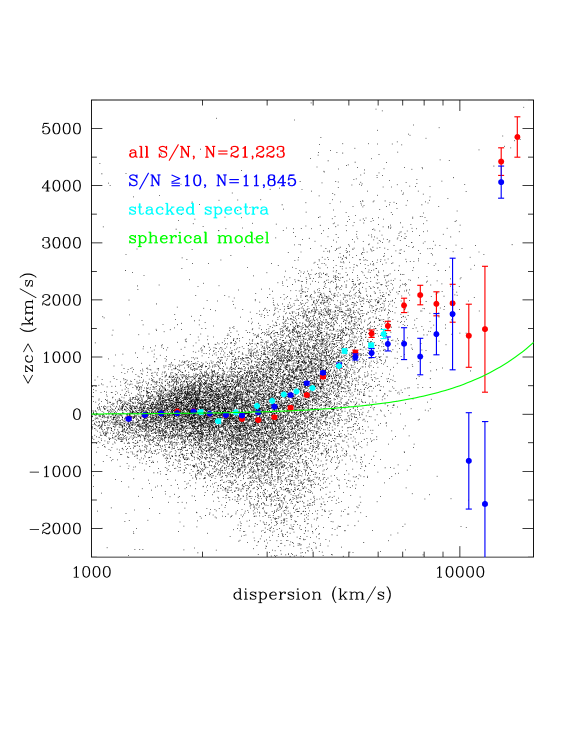
Figure 1: Mean redshift $\langle z\rangle$ (multiplied by $c$ so units are $\,{\rm km\ s}^{-1}$), versus velocity dispersion $\sigma$ of the broad H$\beta$ line for the SDSS DR7 quasar sample. Points with error bars are means in bins of width 0.05 in $\log_{10}\sigma$. Red points are for the full sample of 21,223 quasars and blue points are for a subset with S/N per pixel $\geq 10$. Cyan points are obtained by fitting to stacked spectra of all quasars within a narrow range of velocity dispersion. The green line shows the predicted redshift for a spherical distribution of clouds (eq. 25).

4 Results

Figure 1 shows a scatter plot of $\langle zc\rangle$ versus $\sigma$ for the quasar sample, as well as the mean redshift $\llangle zc\rrangle_{\sigma}$ for the full sample (red points) and the high-quality sample (blue points). The mean redshifts obtained by stacking spectra in small ranges of dispersion are shown as cyan points. All three sets of points yield very similar relations between dispersion and mean redshift. The green line shows the predicted relativistic mean redshift if the BLR is a spherical, virialized, optically thin distribution of clouds orbiting in the gravitational field of the central BH (eq. 25). The trend in the data is qualitatively similar to the model: the mean redshift is near zero at small dispersions and grows faster than linearly as the dispersion increases, but the model amplitude is too small by a factor of 2–3.

The differences between the mean redshifts in the full sample and the high-quality sample are large and scattered for $\sigma>10,000\,{\rm km\ s}^{-1}$, suggesting that in this dispersion range the sample contains very little information for our purposes—there are only 32 quasars with $\sigma>10,000\,{\rm km\ s}^{-1}$ in the full sample, and only 11 in the high-quality sample—so we drop these from the analysis. We also drop quasars with $\sigma<1300\,{\rm km\ s}^{-1}$ from the sample, since this dispersion range may be affected by the cut in the line width used in constructing the SDSS quasar catalog, as discussed in §3.

We next fit these data to the disk models described in §2.3. We adopt the simplest parametrization of the unification model, in which disks are obscured and hence invisible if and only if the inclination of the disk axis to the line of sight exceeds $I_{\rm max}$ (eq. 33). For optically thick disks (e.g., accretion disks), we have two free parameters: $I_{\rm max}$ and the intrinsic velocity dispersion $s$ within the disk. The expected relation between the dispersion and the mean redshift is then given by equation (35); the distribution of rms circular speeds $u=\langle v^{2}\rangle^{1/2}$, $P(u)$ in that equation, is obtained by inverting the integral equation (31) that relates $P(u)$ to the distribution of dispersions $p(\sigma)$ over the range $1300\,{\rm km\ s}^{-1}<\sigma<10,000\,{\rm km\ s}^{-1}$. In practice this inversion is done by modeling $P(u)$ as the sum of 20–30 Gaussians in $\log u$; the means are equally spaced in $\log u$ and the standard deviations and normalizations are adjusted to minimize $\chi^{2}$ between $p(\sigma)$ and the distribution of dispersions in the quasar sample (Fig. 2). The median measurement error on $\sigma$ is $\sim 350\,{\rm km\ s}^{-1}$, which is small compared to the typical dispersion and therefore is not modeled in $\chi^{2}$, i.e., the errors are taken to be the Poisson errors in the number of quasars in each dispersion bin. The fitting procedure for optically thin disks (e.g., disks composed of emitting clouds) is similar: there are two free parameters, $I_{\rm max}$ and the radial velocity dispersion $s_{R}$, and we set the anisotropy parameters to $f_{\phi}=f_{z}=0.5$.

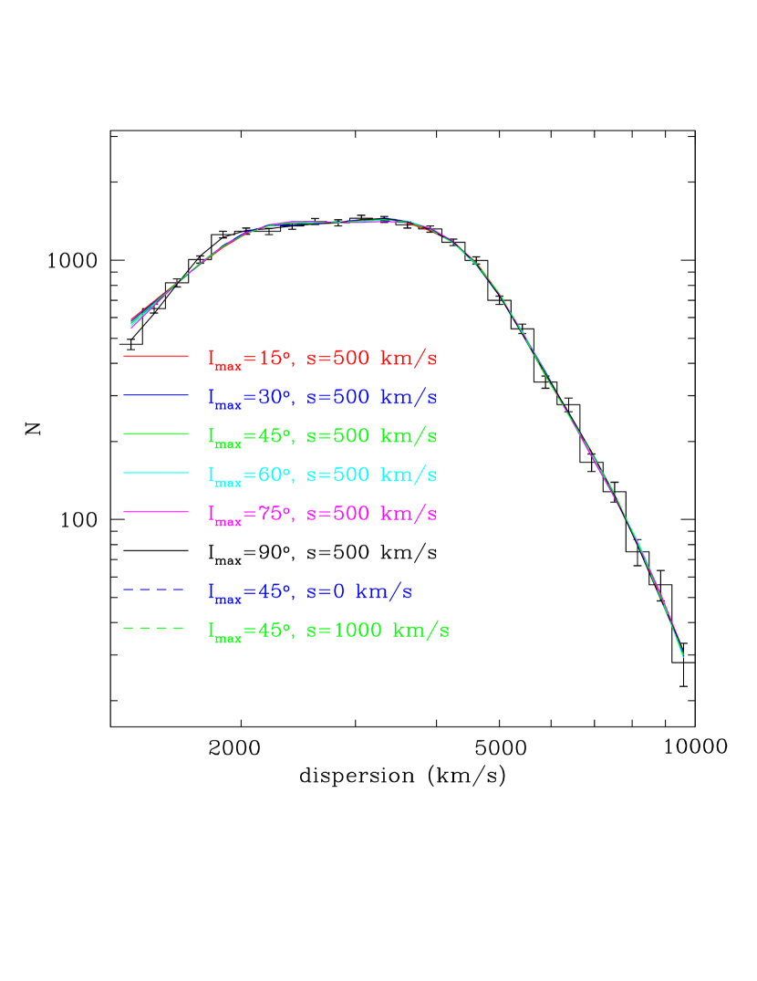
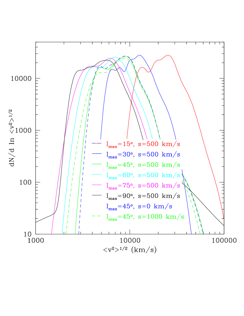
Figure 2: (Left) Distribution of dispersions in the full sample of quasars (histogram) along with fits to optically thick disk models with different values of the disk dispersion $s$ and the maximum unobscured inclination $I_{\rm max}$ (eq. 34). The fits are obtained by modeling the distribution of rms circular speeds $u=\langle v^{2}\rangle^{1/2}$ as a sum of Gaussians in $\log u$. (Right) The corresponding distributions in rms circular speed. The wiggles in the distributions arise because we are solving an ill-conditioned integral equation.

Figure 3 shows the predicted values of the mean redshift for the full and high-quality samples in optically thick disks (the predicted values are slightly different in the two samples because they depend on the fit to the distribution of dispersions in each sample). The solid curves are for maximum inclinations $I_{\rm max}=15^{\circ},30^{\circ},\ldots,75^{\circ},90^{\circ}$ with intrinsic disk dispersion $s=500\,{\rm km\ s}^{-1}$. We also show predictions with $I_{\rm max}=45^{\circ}$ and intrinsic dispersions of 0 and $1000\,{\rm km\ s}^{-1}$ (dashed lines). Figure 4 shows similar results for optically thin disks using the full sample.

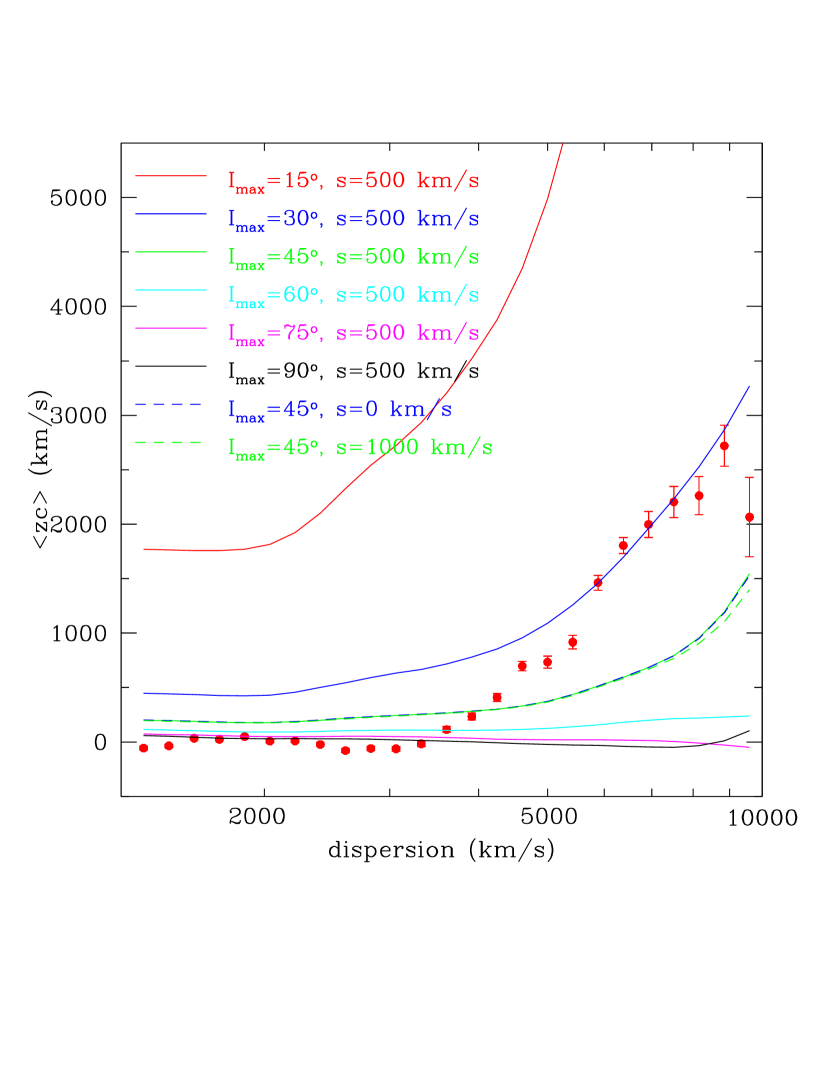
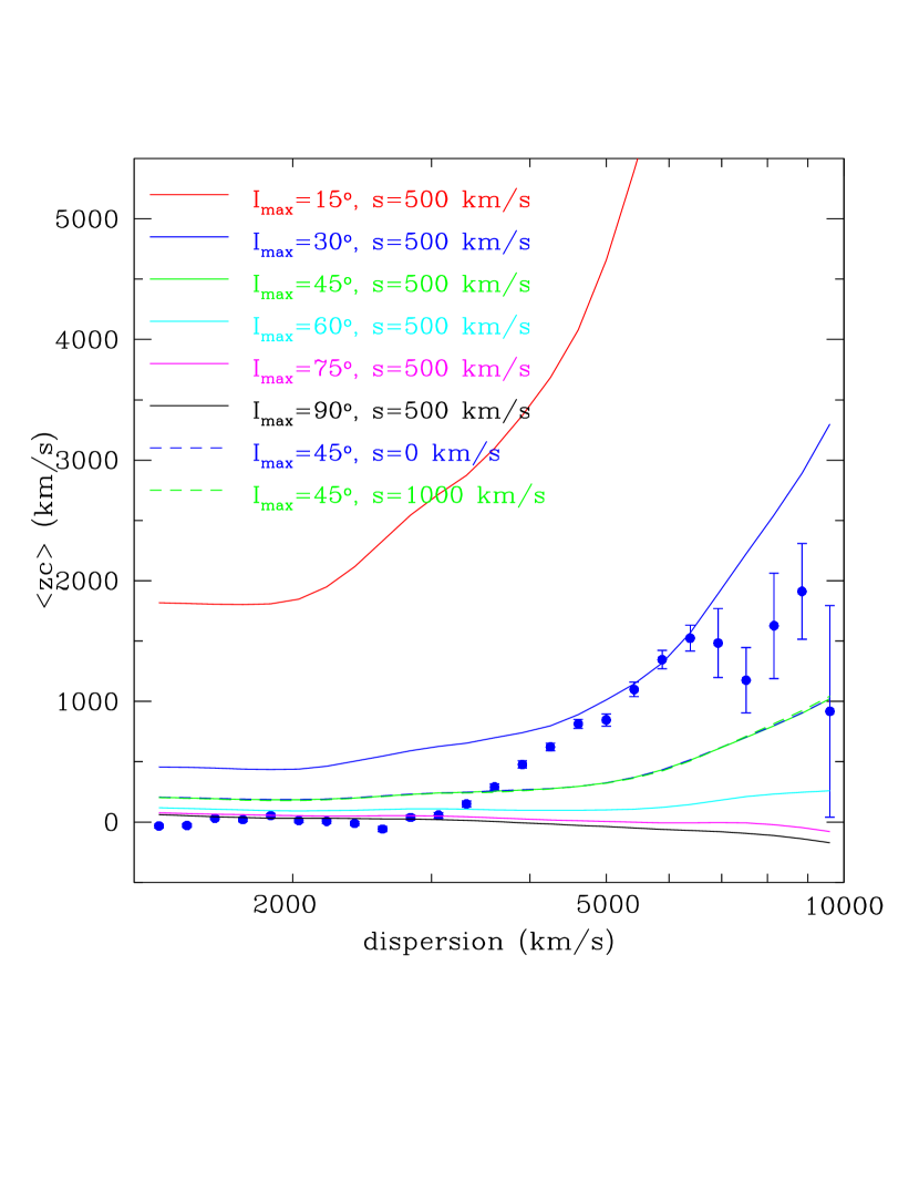
Figure 3: Predicted mean redshift due to relativistic effects in the full quasar sample (left) and the high-quality sample (right). Optically thick disk models with intrinsic dispersion $s=500\,{\rm km\ s}^{-1}$ and a range of maximum unobscured inclinations $I_{\rm max}$ are denoted by solid lines, and models with $I_{\rm max}=45^{\circ}$ and a range of intrinsic dispersions are shown as dashed lines—these are difficult to distinguish because they almost coincide.

At low dispersions, $\sigma\lesssim 2500\,{\rm km\ s}^{-1}$, the data exhibit very small mean redshifts, typically a few tens of $\,{\rm km\ s}^{-1}$ (see footnote 7). This result favors disk models with large $I_{\rm max}$, since the redshift at low dispersions declines as $I_{\rm max}$ increases (for example, when $I_{\rm max}=75^{\circ}$ the mean redshift in our models for $\sigma<2500\,{\rm km\ s}^{-1}$ is $\sim 60\,{\rm km\ s}^{-1}$). At higher dispersions these models work much less well, producing mean redshifts that are far smaller than those in the data, or even negative redshifts.

Models with small $I_{\rm max}$, in particular $I_{\rm max}=15^{\circ}$, predict redshifts that are larger than the observations by several thousand $\,{\rm km\ s}^{-1}$. In addition, such models are in tension with BH masses estimated by other methods. The model with $I_{\rm max}=15^{\circ}$ requires a typical circular speed $\langle v^{2}\rangle^{1/2}\simeq 20,000\,{\rm km\ s}^{-1}$ for our quasar sample (right panel of Figure 2). Combining this with the typical BLR size estimated from the optical luminosity using the empirical relation determined from RM (e.g., Bentz et al., 2009), $R_{\rm BLR}\simeq 0.06$ pc, implies a typical BH mass of $6\times 10^{9}\,M_{\odot}$ for our quasar sample. This is an order of magnitude larger than the virial BH mass estimates based on the average conversion factor between the line width and rms velocity, which is empirically calibrated using the relation between BH mass and stellar velocity dispersion (Shen, 2013; Kormendy & Ho, 2013).

In contrast to the unsatisfactory agreement for large or small values of the maximum opening angle $I_{\rm max}$, all the data for $\sigma\gtrsim 3500\,{\rm km\ s}^{-1}$ is bracketed by the model curves for disks with $I_{\rm max}$ in the range 30–45^∘. Compared to the strong effect of the maximum inclination, the intrinsic disk dispersion $s$ has almost no effect: the three curves for $I_{\rm max}=45^{\circ}$ with intrinsic dispersions ranging from 0 to $1000\,{\rm km\ s}^{-1}$ lie almost on top of one another in Figure 3. The differences between optically thick and thin disks are also small.

Given the likely systematic errors in fitting the mean redshift and dispersion of the broad H$\beta$ line, we believe that Figure 3 suggests strongly that (i) the mean broad-line redshift in a large sample of similar quasars arises mostly from relativistic effects; (ii) the BLR gas orbits in a steady-state disk configuration (or some other configuration whose mean redshift mimics that of a disk); (iii) the distribution of disk orientations is not isotropic, and can be approximated as an initially isotropic distribution from which disks with inclination to the line of sight $\gtrsim 45^{\circ}$ are removed. These conclusion are independent of, but consistent with, AGN unification models, in which Type 2 AGN arise when a central disk is blocked by an obscuring torus. The maximum inclination $I_{\rm max}=45^{\circ}$ corresponds to the half-opening angle of the torus, and it is remarkable that the value derived from our analysis is roughly consistent with values derived from studies of AGN demographics and multi-wavelength data. For example, Schmitt et al. (2001) study a sample of infrared-selected Seyfert galaxies and estimate $I_{\rm max}=48^{\circ}$ from the fraction of obscured (Type 2) Seyferts, which should equal $\cos I_{\rm max}$. Polletta et al. (2008) estimate a somewhat larger half-opening angle, $\sim 67^{\circ}$, in a sample of luminous infrared-selected quasars; while Roseboom et al. (2013) find the 1–$\sigma$ confidence interval of the distribution of opening angles to be $52^{\circ}<I_{\rm max}<76^{\circ}$. Using polarization measurements, Marin (2014) finds that the transition between Type 1 and Type 2 is at inclinations between $45^{\circ}$ and $60^{\circ}$.

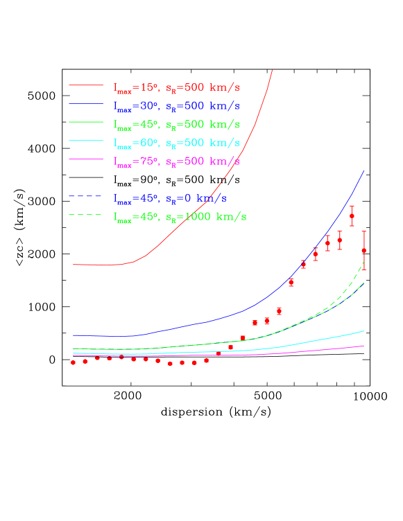
Figure 4: As in the left panel of Fig. 3, but for optically thin disks.

5 Caveats and tests

The discrepancies between our best models and the data may arise from several causes:

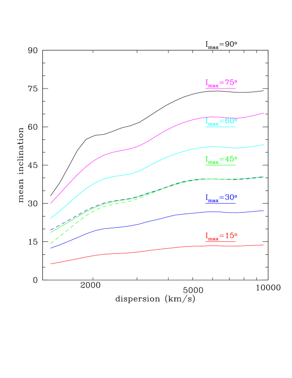
Figure 5: Mean inclination versus dispersion for the optically thick disk models shown in the left panel of Figure 3. The short horizontal lines indicate the opening angle $I_{\rm max}$ for the models of the same color. Note that the mean inclination is correlated with velocity dispersion.

1. Systematic errors in our fits for the velocity dispersion and mean velocity. In this case we expect that more sophisticated analyses would yield better matches between the observations and models in plots like Figure 3.

2. Failure of our assumption that the BLR gas kinematics is dominated by the gravity of the BH and is in virial equilibrium, perhaps because of inflows or outflows, which may be present in some or all BLRs. The approximate agreement that we have observed between the observed mean redshifts and the predictions of simple disk models based on circular orbits sets strong constraints on the average inflow/outflow. As an example, suppose that the disk lies in the equatorial plane of a cylindrical $(R,\phi,z)$ coordinate system and that the disk is optically thick so only material with $z>0$ is visible to the observer. We may model the velocity field of the disk material as

   $${\bf v}=v(R)[\hat{}\mbox{\boldmath$\phi$}+w_{R}\hat{\bf R}+w_{z}\mbox{\,sgn}(z)\hat{\bf z}];$$ (39)

   here $v(R)$ is the circular speed and the dimensionless factors $w_{R}$ and $w_{z}$ represent the outflows in the radial and normal directions. If the inclination between the line of sight and the disk axis is $I$, then the mean redshift is

   $$\langle zc\rangle=-v(R)w_{z}\cos I.$$ (40)

   If the intrinsic dispersion $s$ in the disk is small compared to $v(R)$ then equation (29) gives

   $$w_{z}=-\frac{\langle zc\rangle}{\sqrt{2}\sigma}\frac{\langle v^{2}\rangle^{1/2}}{\langle v\rangle}\tan I=-0.035\frac{\langle zc\rangle}{100\,{\rm km\ s}^{-1}}\frac{2000\,{\rm km\ s}^{-1}}{\sigma}\frac{\langle v^{2}\rangle^{1/2}}{\langle v\rangle}\tan I.$$ (41)

   Thus the sample-averaged BLR inflow/outflow velocity must either be much smaller than the circular speed, or nearly in the equatorial plane of the disk.

3. Failure of our assumption that the core of narrow [O iii] line equals the systemic velocity, and that this in turn equals the BH velocity. This is unlikely since the core [O iii] component agrees with the systemic velocity estimated from stellar absorption to within $50\,{\rm km\ s}^{-1}$ in cases where both can be measured (Hewett & Wild, 2010).

4. Failure of our model for the obscuration, in which a quasar appears in the sample if and only if its inclination to the line of sight is less than the opening angle $I_{\rm max}$ (eq. 33). This model is probably too simple: (i) It is likely that the opening angle $I_{\rm max}$ of the obscuring torus has some distribution among different quasars with otherwise similar properties (e.g., Elitzur, 2012); in this case there is no hard threshold of inclination above which all (broad-line) quasars are obscured. (ii) The torus opening angle distribution may be a function of quasar luminosity or Eddington ratio (e.g., Simpson, 2005; Lusso et al., 2013). (iii) The torus may not be entirely opaque, for example if it is composed of discrete clouds with a covering factor $\lesssim 1$. The quality and quantity of the available data are not sufficient to discriminate between these possibilities using relativistic effects. We have experimented with other models for the obscuration, but have not found any that match the data in Figures 3 and 4 significantly better. We have, however, found otherwise plausible models that are worse, which leads us to hope that fitting mean redshifts to relativistic models may eventually offer valuable constraints on models of the obscuring torus.

5. Failure of our assumption that the joint distribution in rms circular speed $u=\langle v^{2}\rangle^{1/2}$ and inclination $I=\cos^{-1}\nu$ is separable, i.e., the assumption that $P(u,\nu)=P(u)Q(\nu)$. Note that although the distribution of rms circular speed and inclination is separable, the distribution of dispersion and inclination is not (Figure 5). Quasars with high dispersions are more nearly edge-on.

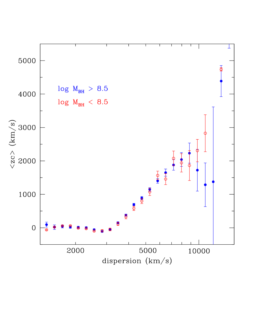
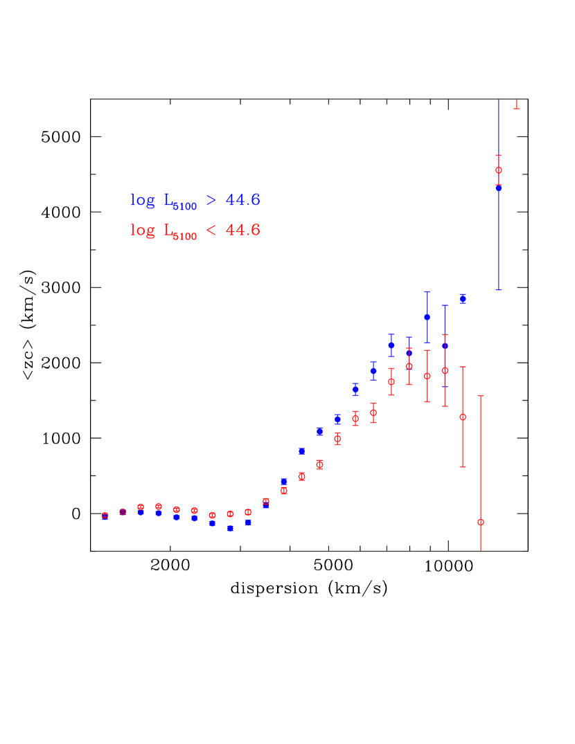
Figure 6: Mean redshift versus dispersion of the broad H$\beta$ line. Left panel: the quasar sample has been split into high and low BH mass subsamples, each with equal numbers of quasars (blue and red points respectively). Right panel: a similar split into high- and low-luminosity subsamples. The masses and luminosities are from Shen et al. (2011).

One consistency check of our simple model is that the relation between mean redshift and velocity dispersion should not depend strongly on other parameters of the quasar, such as BH mass or luminosity. To carry out this check we use virial estimates of the black-hole mass $M_{\bullet}$ (eq. [5] of Vestergaard & Peterson 2006) from the catalog of Shen et al. (2011), and divide the quasar sample into high and low BH mass subsamples at the median mass, given by $\log M_{\bullet}/M_{\odot}=8.51$. The results are shown in the left panel of Figure 6 as blue (high-mass) and red (low-mass) points. There are no significant systematic differences between the high- and low-mass samples. The differences in mean redshifts between the two subsamples are generally about what is expected from the statistical uncertainties. The velocities in the low-mass subsample are systematically higher in the bins with dispersion $\gtrsim 10^{4}\,{\rm km\ s}^{-1}$, but these contain only a handful of quasars (38 in the high-mass subsample and 21 in the low-mass subsample). Thus there is no evidence that the relation between mean redshift and dispersion depends on BH mass.

Next we divide the sample into high- and low-luminosity subsamples at the median continuum luminosity, given by $\log L_{5100}/\mbox{erg s}^{-1}=44.63$ with $L_{5100}$ taken from the same catalog. The results are shown in the right panel Figure 6 as blue (high-luminosity) and red (low-luminosity) points. The differences between the two subsamples are small but significant: the low-luminosity sample has larger mean redshifts for dispersion $\sigma<3500\,{\rm km\ s}^{-1}$, and smaller redshifts for larger dispersions (for comparison, the ratio of the median luminosities of the two subsamples is $\Delta\log L=0.54$). The reason for these differences is not clear. One possibility is that the opening angle of the obscuring torus depends on the quasar luminosity; there is evidence that the opening angle is larger in quasars with larger luminosity (e.g., Simpson, 2005; Lusso et al., 2013). A second possibility is that more luminous quasars are biased towards more face-on systems, either because these suffer from less extinction or because the luminosity of an optically thick, geometrically thin disk varies as $\cos I$. The first of these effects would produce a mean redshift that is smaller at all dispersions in the high-luminosity sample, while the second would produce a mean redshift that is larger at high luminosities (cf. Figure 3). In any event the difference in mean redshift between the low-luminosity and high-luminosity samples is much smaller than the overall trend, which supports the conclusion that this trend is not determined primarily by the quasar luminosity.

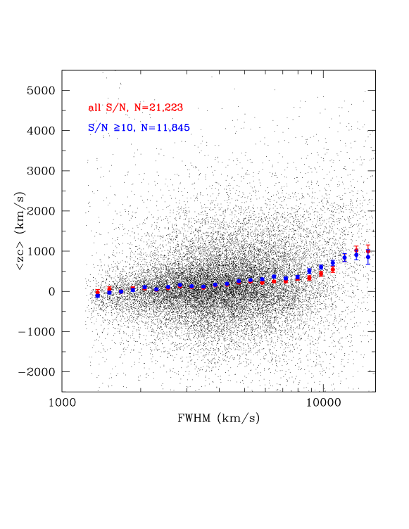
Figure 7: Same as Figure 1, except FWHM is used instead of dispersion as a measure of the width of the H$\beta$ line.

The full-width at half-maximum (FWHM) is generally regarded as a more stable measure of the width of quasar broad lines than the dispersion (e.g., Shen, 2013). We do not use FWHM because it does not have simple relations to $\langle v\rangle$ of the kind derived in §2.1. Nevertheless, it is instructive to plot the mean redshift as a function of FWHM (Figure 7). The same general trend of increasing redshift with increasing width is seen; however, the curve is smoother—as we might expect if FWHM is a more stable measure of the velocity width—and rises only to $\langle v\rangle\simeq 1000\,{\rm km\ s}^{-1}$ at FWHM$\simeq 15,000\,{\rm km\ s}^{-1}$ compared to $\langle v\rangle\simeq 1500$–$2000\,{\rm km\ s}^{-1}$ at $\sigma\simeq 15,000\,{\rm km\ s}^{-1}$. This difference in the dependence of mean redshift on $\sigma$ and FWHM is actually expected: for the broad H$\beta$ line, the ratio FWHM$/\sigma$ is known to increase with line width (e.g., Peterson, 2011; Kollatschny & Zetzl, 2011). It has long been suggested that the line shape (FWHM$/\sigma$ ratio) is an indicator of the orientation of the BLR (e.g., Collin et al., 2006). In such a scenario, the BLR has two components: a flattened component (i.e., a thin disk), and an isotropic component (either from isotropic turbulence in the disk or from a separate, spherical component of the BLR). The FWHM mainly measures the core of the line, and is more sensitive to the disk component, while $\sigma$ is more sensitive to the isotropic component in the line wings. Thus larger FWHM$/\sigma$ ratios are biased towards more edge-on (higher inclination) systems. Our approach outlined in §2 automatically takes into account the orientation bias in line width.

The mean redshift among the low-dispersion quasars in our sample ($\sigma\leq 2500\,{\rm km\ s}^{-1}$, 46% of the sample) is only $\langle zc\rangle=10\pm 6\,{\rm km\ s}^{-1}$, consistent with zero. Therefore if there are substantial systematic errors or inflows/outflows, then either two or more effects cancel (e.g., the redshift from relativistic effects cancels the blueshift from an outflow), which seems unlikely but not impossible, or inflows/outflows in the broad- and narrow-line components and systematic errors all contribute less than a few tens of $\,{\rm km\ s}^{-1}$ to the mean redshift for $\sigma\lesssim 2500\,{\rm km\ s}^{-1}$. In particular, if the sample-averaged blueshift from an outflow is less than $10\,{\rm km\ s}^{-1}$, equation (41) implies that the sample-averaged outflow velocity perpendicular to the disk is less than $w_{z}\sim 0.3\%$ of the local circular speed.

Figure 8: Eddington ratio $L_{5100}/L_{\rm Edd}$ for the quasar sample, where $L_{5100}$ is the continuum luminosity and $L_{\rm Edd}$ is the Eddington luminosity based on a virial estimate of the BH mass.

A further complication is that our quasar sample includes a range of Eddington ratios $L/L_{\rm Edd}$, as plotted in Figure 8. Here the BH mass $M_{\bullet}$ and continuum luminosity $L_{5100}$ are computed as described in §5 and the Eddington luminosity $L_{\rm Edd}=1.5\times 10^{38}\mbox{\, erg s}^{-1}\,M_{\bullet}/M_{\odot}$. The quasars with low dispersion typically have larger Eddington ratios. If outflows are preferentially launched in quasars with high Eddington ratios, then objects with smaller dispersions may be more biased to outflows, which will lower the mean redshift. This effect might alleviate the discrepancy between the near-zero mean redshift that is observed for $\sigma\lesssim 2500\,{\rm km\ s}^{-1}$ and the predictions of disk models with $I_{\rm max}\sim 30^{\circ}$–$45^{\circ}$ (Figs. 3 and 4). Consistent with this suggestion, the quasars in our sample with $\sigma<2500\,{\rm km\ s}^{-1}$ exhibit a weak dependence of mean redshift with Eddington ratio: the lowest quartile ($L/L_{\rm Edd}<0.0093$) has $\langle zc\rangle=53\pm 10\,{\rm km\ s}^{-1}$ and the highest quartile ($L/L_{\rm Edd}>0.0286$) has $\langle zc\rangle=-91\pm 10\,{\rm km\ s}^{-1}$.

6 Summary

Using data from the SDSS DR7 quasar catalog, we have argued that the mean redshift in quasar broad-line regions (BLRs) is largely due to relativistic effects. The data then suggest that the BLR kinematics is described approximately by a disk that is obscured when its inclination to the line of sight exceeds $I_{\rm max}\sim 30^{\circ}$–$45^{\circ}$, and that outflow or infall has only a small effect on the mean redshift.

Our results strengthen the credibility of virial or single-epoch estimates of BH masses in broad-line AGN (e.g., Shen, 2013), which rely on the assumption that the BLR is in virial equilibrium, and also provide guidance on the geometry and kinematics of the BLR, which are needed to calibrate these mass estimates.

What do we need to improve the constraints provided by this approach? A sample with more quasars, or higher quality spectra, or a larger dynamic range in luminosity would help although the Poisson errors are already small and we do not see any strong dependence of the mean redshift on signal-to-noise ratio or luminosity. Probably the largest potential source of systematic error is in modeling the mean redshift and dispersion, and more sophisticated spectral fits might lead to better agreement between the observed mean redshift vs. dispersion relation and the simple theoretical models presented here. It would be worthwhile to extend the analysis to other broad lines, in particular MgII, although the spectral modeling is more difficult for this line and there are no SDSS [O iii] or [O ii] redshifts to provide systemic velocities beyond $z=1.5$. Finally, more general theoretical models of the kinematics of the BLR and the geometry of the obscuration may provide better fits to the data.

Our working hypothesis has been that the mean redshifts in large samples of quasars with similar properties are due to relativistic effects in a steady-state, virialized, broad-line region. Further investigation of this hypothesis should lead to new insights about the nature of the broad-line region and the properties of the obscuring torus and other quasar components.

References

- Antonucci (1993) Antonucci, R. 1993, ARA&A, 31, 473
- Bentz et al. (2009) Bentz, M. C., Peterson, B. M., Netzer, H., Pogge, R. W., & Vestergaard, M. 2009, ApJ, 697, 160
- Binney & Tremaine (2008) Binney, J., & Tremaine, S. 2008, Galactic Dynamics (2nd ed.) Princeton University Press, Princeton, NJ.
- Chen et al. (1989) Chen, K., Halpern, J. P., & Filippenko, A. V. 1989, ApJ, 339, 742
- Collin et al. (2006) Collin, S., Kawaguchi, T., Peterson, B. M., & Vestergaard, M. 2006, A&A, 456, 75
- Cunningham (1975) Cunningham, C. T. 1975, ApJ, 202, 788
- Dumont & Collin-Souffrin (1990) Dumont, A. M., & Collin-Souffrin, S. 1990, A&A, 229, 313
- Elitzur (2012) Elitzur, M. 2012, ApJ, 747, L33
- Eracleous (1999) Eracleous, M. 1999, in Structure and Kinematics of Quasar Broad Line Regions, ASP Conference Series, 175, Astronomical Society of the Pacific, San Francisco, p. 163
- Eracleous & Halpern (2003) Eracleous, M., & Halpern, J. P. 2003, ApJ, 599, 886
- Eracleous et al. (1995) Eracleous, M., Livio, M., Halpern, J. P., & Storchi-Bergmann, T. 1995, ApJ, 438, 610
- Gerbal & Pelat (1981) Gerbal, D., & Pelat, D. 1981, A&A, 95, 18
- Ginzburg & Syrovatskii (1969) Ginzburg, V. L., & Syrovatskii, S. I. 1969, ARA&A, 7, 375
- Hewett & Wild (2010) Hewett, P. C., & Wild, V. 2010, MNRAS, 405, 2302
- Kaiser (2013) Kaiser, N. 2013, MNRAS, 435, 1278
- Kollatschny (2003) Kollatschny, W. 2003, A&A, 412, L61
- Kollatschny & Zetzl (2011) Kollatschny, W., & Zetzl, M. 2011, Nature, 470, 366
- Kormendy & Ho (2013) Kormendy, J., & Ho, L. C. 2013, ARA&A, 51, 511
- Laor (2006) Laor, A. 2006, ApJ, 643, 112
- Lusso et al. (2013) Lusso, E., et al. 2013, ApJ, 777, 86
- Marin (2014) Marin, F. 2014, MNRAS, 441, 551
- McIntosh et al. (1999) McIntosh, D. H., Rix, H.-W., Rieke, M. J., & Foltz, C. B. 1999, ApJ, 517, L73
- Pancoast et al. (2013) Pancoast, A., et al. 2013, arXiv:1311.6475
- Peterson (2011) Peterson B. M., 2011, in Narrow-Line Seyfert 1 Galaxies and their Place in the Universe, Proceedings of Science, vol. NLS1, 32
- Peterson et al. (2004) Peterson, B. M., et al. 2004, ApJ, 613, 682
- Polletta et al. (2008) Polletta, M., Weedman, D., Hönig, S., et al. 2008, ApJ, 675, 960
- Roseboom et al. (2013) Roseboom, I. G., Lawrence, A., Elvis, M., et al. 2013, MNRAS, 429, 1494
- Runnoe et al. (2013) Runnoe, J. C., et al. 2013, MNRAS, 429, 135
- Rybicki & Lightman (1979) Rybicki, G. B., & Lightman, A. P. 1979, Radiative Processes in Astrophysics, John Wiley & Sons, New York.
- Schmitt et al. (2001) Schmitt, H. R., Antonucci, R. R. J., Ulvestad, J. S., et al. 2001, ApJ, 555, 663
- Schneider et al. (2010) Schneider, D. P., et al. 2010, AJ, 139, 2360
- Shen (2013) Shen, Y. 2013, Bulletin of the Astronomical Society of India, 41, 61
- Shen et al. (2008) Shen, Y., Greene, J. E., Strauss, M. A., Richards, G. T., & Schneider, D. P. 2008, ApJ, 680, 169
- Shen et al. (2011) Shen, Y., et al. 2011, ApJS, 194, 45
- Simpson (2005) Simpson, C. 2005, MNRAS, 360, 565
- Strateva et al. (2003) Strateva, I. V., et al. 2003, AJ, 126, 1720
- Urry & Padovani (1995) Urry, C. M., & Padovani, P. 1995, PASP, 107, 803
- Vestergaard & Peterson (2006) Vestergaard, M., & Peterson, B. M. 2006, ApJ, 641, 689
- Wills & Browne (1986) Wills, B. J., & Browne, I. W. A. 1986, ApJ, 302, 56
- Zheng & Sulentic (1990) Zheng, W., & Sulentic, J. W. 1990, ApJ, 350, 512