Numerical simulations of dwarf galaxy merger trees

Abstract

We investigate the evolution of dwarf galaxies using $N$-body/SPH simulations that incorporate their formation histories through merger trees constructed using the extended Press-Schechter formalism. The simulations are computationally cheap and have high spatial resolution. We compare the properties of galaxies with equal final mass but with different merger histories with each other and with those of observed dwarf spheroidals and irregulars.

We show that the merger history influences many observable dwarf galaxy properties. We identify two extreme cases that make this influence stand out most clearly: (i) merger trees with one massive progenitor that grows through relatively few mergers and (ii) merger trees with many small progenitors that merge only quite late. At a fixed halo mass, a type (i) tree tends to produce galaxies with larger stellar masses, larger half-light radii, lower central surface brightness, and since fewer potentially angular momentum cancelling mergers are required to build up the final galaxy, a higher specific angular momentum, compared with a type (ii) tree.

We do not perform full-fledged cosmological simulations and therefore cannot hope to reproduce all observed properties of dwarf galaxies. However, we show that the simulated dwarfs are not unsimilar to real ones.

1 Introduction

Numerical simulations of individual dwarf galaxies have several advantages over full-fledged cosmological simulations: one can achieve very high spatial resolution and one has full control over the initial conditions, provided the latter are sufficiently realistic and cosmologically motivated. Thus, it can be easier to study the impact of certain physical parameters, such as mass or angular momentum, on the evolution of a galaxy. However, real galaxies obviously do not evolve in isolation from the rest of the Universe. For one, according to current cosmological theory, even dwarf galaxies have formed through a series of mergers in a bottom-up fashion.

Isolated dwarf galaxy simulations are not computationally demanding, have a well determined initial set-up, and can achieve high spatial resolution. They can be extended to also include ram-pressure stripping or interactions with a massive neighbor (Mayer et al., 2001b). Such simulations have shown that the total galaxy mass is the main parameter determining the appearance and evolution of dwarf galaxies (Valcke, De Rijcke & Dejonghe, 2008; Revaz et al., 2009; Sawala et al., 2010). Schroyen et al. (2011) suggest angular momentum as a crucial second parameter that determines individual star formation modes and offers an explanation for the observed metallicity gradients (Tolstoy et al., 2004; Koleva et al., 2009; Tolstoy, Hill & Tosi, 2009; Kirby et al., 2011; Battaglia et al., 2011).

Supposedly more realistic simulations of dwarf galaxies can be obtained from large ab initio cosmological simulations. However, due to their low mass, the dwarf galaxies in such simulations are often seriously undersampled making it difficult to produce robust predictions for their observational properties (Sawala et al., 2011). For example, the dark matter particle mass in the Millennium simulation (Springel et al., 2005) and the Millennium-II simulations (Boylan-Kolchin et al., 2009) is, respectively, 8.6$\times$10⁸ h^-1 M_⊙ and 6.88$\times$10⁶ h^-1 M_⊙. Similarly the Bolshoi simulations (Klypin, Trujillo-Gomez & Primack, 2011) have a mass resolution of 1.35$\times$10⁸ h^-1 M_⊙. Given that dwarfs with masses similar to the Local Groups dwarfs contain only 10 to 100 dark matter particles, and their progenitors even less, their merger histories will be very poorly described by these simulations. Also, the identification of haloes in large cosmological simulations is not straightforward and the resulting merger trees can be different depending on which halo finder method is used (Srisawat et al., 2013). Moreover, one has no handle on the number or the properties (e.g. final mass) of the formed dwarfs. A significant improvement over this is to re-simulate a small part of a cosmological simulation box to follow the formation and evolution of a dwarf galaxy of interest in full detail (Governato et al., 2010; González-Samaniego et al., 2013). Unfortunately, this requires two simulations to be run and is therefore a computationally expensive endeavor.

In this paper, we present a third way of producing more cosmologically sound dwarf galaxy simulations. The Press-Schechter (PS) formalism (Press & Schechter, 1974) uses the spherical collapse model, which is a simple model for the nonlinear structure formation in the Universe, to derive the conditional mass function. The extended Press-Schechter (EPS) theory (Bond et al., 1991; Lacey & Cole, 1993) or excursion set approach uses this conditional mass function to estimate the rate at which smaller objects merge into larger objects or the halo formation distribution. With the help of Monte Carlo algorithms a merger tree can be constructed in a top-down fashion starting from its final mass. There are many algorithms available to investigate structure formation based on this method. A detailed comparison of existing Monte Carlo algorithms and a general overview of the EPS theory can be found in Zhang, Fakhouri & Ma (2008), along with a comparison of the algorithms of Kauffmann & White (1993); Lacey & Cole (1993); Somerville & Kolatt (1999); Cole et al. (2000) and three new algorithms. However, the results of the algorithms that use EPS overpredict the abundance of small haloes and underpredict the abundance of larger haloes with increasing redshift compared to the result of the cosmological $N$-body simulations (Lacey & Cole, 1994; Tormen, 1998; Sheth & Tormen, 1999; Zhang, Fakhouri & Ma, 2008). This is likely due to the “spherical” approximation which is used in EPS while real haloes are rather triaxial (Bardeen et al., 1986). But, as the results from the spherical collapse model produce merger trees with statistical properties which have the same trends with mass and redshift as merger trees from the Millennium simulation, Parkinson, Cole & Helly (2008) adapted the GALFORM algorithm of Cole et al. (2000) to fit the conditional mass function of the Millennium simulation.

We propose to use EPS to produce a merger tree that fixes the timing of the mergers leading up to a galaxy of a given mass at $z=0$. The orbital parameters of the individual mergers are sampled from probability distribution functions derived from cosmological simulations. We then use an $N$-body/SPH code to simulate in full detail the merger sequence and the build-up and evolution of the galaxy. Using this approach, one is able to build simulated galaxies in a more cosmologically realistic way while retaining some of the benefits of the isolated-galaxy simulations, such as high resolution and control over the final galaxy mass.

In section 2, we provide more details about the numerical methods in the code that was used to simulate dwarf galaxies. An analysis of the simulations is given in section 3, where our models are compared with observations in terms of their location on the observed kinematic and photometric scaling relations. In section 4 we discuss the obtained results and we formulate our conclusions in section 5.

2 Simulations

For the simulations we use a modified version of the $N$-body/SPH code Gadget-2 (Springel, 2005). This code is extended with star formation, feedback and metal dependent radiative cooling. In the past, this code has been used by our group to simulate isolated dwarf galaxy models with cosmologically motivated initial conditions, meaning a NFW halo (Navarro, Frenk & White, 1996) for the dark matter, a baryon fraction in agreement with the cosmological model, etc. The results of these simulations are discussed in Valcke, De Rijcke & Dejonghe (2008), Valcke et al. (2010), Schroyen et al. (2011), Cloet-Osselaer et al. (2012), and Schroyen et al. (2013). From these studies we can conclude that the isolated models are in agreement with the kinematic and photometric scaling relations of observed dwarf galaxies and the results of other simulations (Revaz et al., 2009; Sawala et al., 2010).

We build on our experience with isolated models in order to construct a dwarf galaxy with a hierarchical structure formation history. First, we construct a merger tree (see paragraph 2.3) whose leaves are populated with isolated dwarf galaxy models with cosmologically motivated initial conditions (ICs) (see paragraph 2.1). These protogalaxies are then evolved and merged using the $N$-body/SPH code (see paragraph 2.2).

As for our isolated simulations we do not aim to specifically simulate either late-type or early-type dwarfs. The classification of a galaxy would in any case depend on the presence of gas-removing processes, such as ram-pressure stripping, and on when exactly during the star-formation duty cycle the galaxy is observed, as explained in e.g. Schroyen et al. (2013). Given the absence of external gas-removing processes, our simulated galaxies keep their gas until the end and could therefore be classified as late-types. Before this gas removal, there is little reason to suggest that late and early types had a different evolution.

For the visualization and analysis of our results we use our own public available software package HYPLOT. This software is freely available from SourceForge and is used for all the figures in this paper.

2.1 Initial conditions isolated galaxies

We briefly describe the initial setup of the isolated models as each of the members of the merger tree will be setup in isolation. For the dark matter halo an NFW profile is used with a density profile:

$$\rho_{\rm NFW}(r)=\frac{\rho_{\rm s}}{(r/r_{\rm s})(1+r/r_{\rm s})^{2}}$$ (1)

where $\rho_{\rm s}$ and $r_{\rm s}$ are respectively the characteristic density and the scale radius. The Strigari, Kaplinghat & Bullock (2007) relations for the concentration parameter of dwarf dark matter haloes are used for the determination of $\rho_{\rm s}$ and $r_{\rm s}$:

$$c \approx 33\bigg{(}\frac{M_{\rm h}}{10^{8}M_{\odot}}\bigg{)}^{-0.06}$$ (2)

$$\rightarrow \rho_{\rm s}= \frac{101}{3}\ \frac{c^{3}}{\ln(1+c)-c/(1+c)}\ \rho_{c}$$ (3)

$$\rightarrow r_{\rm s}= \bigg{(}\frac{M_{\rm h}}{4\pi\rho_{s}}\frac{1}{\ln(1+c)-c/(1+c)}\bigg{)}^{1/3}$$ (4)

where $\rho_{c}$ is the critical density of the universe at $z=0$ and M_h is the halo mass in units of solar masses. The concentration parameter $c$ is defined as the ratio of the virial radius, r_max, at which the dark matter density profile is cut off, to the scale radius, $r_{s}$. For the gas cloud, we use a pseudo-isothermal density profile. For the detailed implementation of this gas halo we refer to Schroyen et al. (2013). The initial gas metallicity is set to $10^{-4}\ Z_{\odot}$, the initial temperature is $10^{4}$ K. We use a gravitational softening length of 0.03 kpc for all particles.

We use a flat $\Lambda$-dominated cold dark matter cosmology with $h=0.71,\Omega_{\rm tot}=1,\Omega_{\rm m}=0.2383,\Omega_{\rm DM}=0.1967$. The baryonic mass or gas mass in our models is set to be 0.2115 times that of the dark-matter, in accordance to the employed cosmology.

2.2 The code

We use a modified version of the Nbody-SPH code Gadget-2 (Springel, 2005) which is extended by Valcke, De Rijcke & Dejonghe (2008) with star formation, feedback and radiative metallicity dependent cooling. We go trough the implementations of these extensions in the following subsections.

2.2.1 Star formation

Star formation happens in dense, cold and gravitationally collapsing gas regions which are too small to resolve in our simulations, hence, we are forced to implement star formation as a subgrid formalism. In our code, we select star formation regions with the following criteria:

$$\rho_{\rm g} \geq \rho_{\rm SF}$$ (5)

$$T \leq T_{\rm c}=15000\mathrm{K}$$ (6)

$$\vec{\nabla}.\vec{v} \leq 0.$$ (7)

The most important star formation criteria is the first one, the density threshold, for which we use a value of 10 amu cm^-3. This is in agreement with the trend to use a high density threshold in simulations (Governato et al., 2010; Guedes et al., 2011; Cloet-Osselaer et al., 2012; Schroyen et al., 2013) which map the regions of active star formation more accurate. Gas particles that fulfill these criteria can become star particles depending on a Schmidt law. This law connects star formation with the gas density, $\rho_{g}$, the dynamical time, $t_{g}$, and the parameter c_⋆, which is the dimensionless star formation efficiency:

$$\frac{\mathrm{d}\rho_{\rm s}}{\mathrm{d}t}=-\frac{\mathrm{d}\rho_{\rm g}}{\mathrm{d}t}=c_{\star}\frac{\rho_{\rm g}}{t_{\rm g}}.$$ (8)

As shown by other authors (e.g. Stinson et al. (2006); Revaz et al. (2009)) and based on our own experience, there is a wide range of values for the c_⋆ parameter that produces dwarf galaxies with acceptable observable properties and self-regulated star formation. Any value within this range is equally valid. For the simulations presented here we use a value of 0.25 for the c_⋆ parameter, the same value as in Cloet-Osselaer et al. (2012).

By using a high density threshold, star formation occurs more in small gas clumps and is less centrally concentrated, in agreement with observed galaxies (Schroyen et al., 2013).

2.2.2 Feedback and cooling

The code is implemented with feedback from Type Ia supernova (SNIa), Type II supernove (SNII) and stellar winds (SW) as described in Valcke, De Rijcke & Dejonghe (2008). When stars die they deliver thermal energy to the ISM and they enrich the gas. Star particles represent single-age single-metallicity stellar populations (SSP) with a Salpeter initial-mass function (Salpeter, 1955). The feedback is released as thermal feedback to the gas particles close to the star particle, e.g. within the SPH smoothing radius and according to the smoothing kernel of the gas particle the star particle originates from. Massive stars, with low mass limit $m_{SNII,l}=8\ M_{\odot}$ and high mass limit $m_{SNII,h}=60\ M_{\odot}$, die as SNII supernove, while less massive stars, with low mass limit $m_{SNIa,l}=3\ M_{\odot}$ and high mass limit $m_{SNIa,h}=8\ M_{\odot}$, will explode as SNIa explosions. As massive stars will have a short life, they will release their feedback quite fast after a star is born. For the SNIa, we employ a delay of 1.5 Gyr. The total energy released by supernova explosions is set to 10⁵¹ ergs and for stellar winds to 10⁵⁰ ergs. This energy is distributed at a constant rate during their main sequence lifetime. The lifetime is a function of the mass $m$ of the star and is given by (David, Forman & Jones, 1990):

$$\log t(m)=10-3.42\log(m)+0.88(\log(m))^{2}$$ (9)

The energy effectively absorbed by the ISM is obtained by multiplying these energies with the feedback efficiency factor, which is set to 0.7. As discussed in Cloet-Osselaer et al. (2012) there is a degeneracy between the density threshold for star formation and the feedback efficiency factor and as indicated in the previous section, the SN efficiency will also influence the self-regulation of the star formation. From this article, we copied the set of values that has shown to result in dwarf galaxies with properties comparable to real dwarf galaxies. In addition, a high density threshold for star formation in combination with a suitable feedback efficiency partially reduces the final stellar mass of the galaxy which is generally overpredicted in simulations (Scannapieco et al., 2012; Sawala et al., 2011).

For the cooling we use the metallicity-dependent cooling curves from Sutherland & Dopita (1993), which describe the cooling of gas for different metallicities down to a temperature of 10⁴ K. These cooling curves are extended to lower temperatures using the cooling curves of Maio et al. (2007). A particle which is heated by supernova explosion will not be able to cool radiatively during the time-step where the SN explosion occurred, this in order to correct for the fact that our resolution cannot resolve the hot, low density cavities that are generated by the supernova explosions.

$\mathrm{M_{\rm halo}}$	$M_{\rm res}$	$\mathrm{\#DM\ particles}$	$m_{\rm p}$
10$\times$109 M⊙	0.75$\times$108 M⊙	800 000	12 500 M⊙
7.5$\times$109 M⊙	0.50$\times$108 M⊙	400 000	18 750 M⊙
5.0$\times$109 M⊙	0.25$\times$108 M⊙	400 000	12 500 M⊙
2.5$\times$109 M⊙	0.25$\times$108 M⊙	400 000	6 250 M⊙
1.0$\times$109 M⊙	0.1$\times$108 M⊙	400 000	2 500 M⊙

Table 1: Details of the input parameters for the merger trees. In the first column the halo mass is shown, the second column shows the mass resolution which is the smallest possible halo mass. The third column shows the amount of dark matter particles in the simulation and the last column shows the mass of one dark matter particle.

2.3 Merger trees

We have used the GALFORM algorithm (Cole et al., 2000), as modified by Parkinson, Cole & Helly (2008), to construct merger trees. This algorithm is based on the EPS theory which starts from an initial Gaussian random density fluctuation field and uses the analytical model of cosmological spherical collapse to construct a density threshold above which a halo becomes virialized. For a halo of a given mass at a certain redshift, it predicts the conditional mass function of its progenitors at a higher redshift. With Monte Carlo techniques a path can be constructed from the final mass of the galaxy, the root of the tree, to the leaves, which are the smallest galaxies considered in the calculation, at some high redshift. Parkinson, Cole & Helly (2008) adjusted the algorithm to fit the conditional mass function of the Millennium simulation (Springel, 2005). The construction of the merger tree proceeds from its root at $z=0$ to its leaves, which we place at a lookback time of approximately 13.5 Gyr, corresponding to a redshift of $z$=13.5. This redshift interval is divided into 20 bins of equal size. A few examples of the merger trees that are used can be found in Fig. 1. There, the sizes of the circles give an indication of the mass of the haloes.

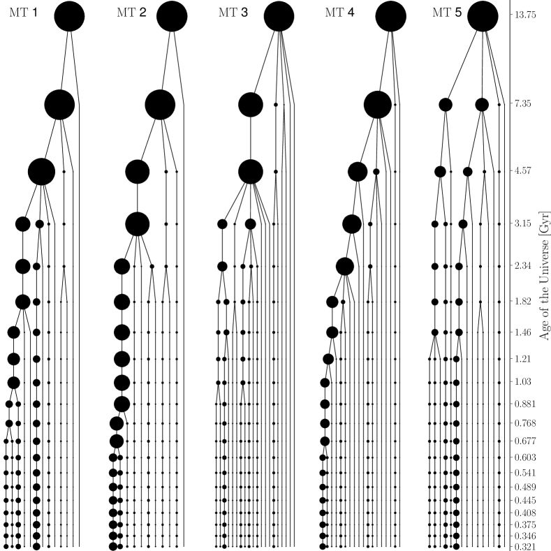
Figure 1: The 5 merger trees of the haloes with a final mass of M_h=2.5$\times$10⁹ M_⊙. The size of the circles gives an indication of the mass of the halo. The evolution is shown as a function of the age of the universe which corresponds with the redshift range from 13.5, when the Universe is 0.32 Gyr old to $z=0$.

As we do not run cosmological simulations, our haloes do not grow in time due to accretion. As visible in the merger trees in Fig. 1, the only way to gain mass is by merging. However, the output of the merger tree algorithm takes mass accretion into account. When the mass growth in a timestep is smaller than some resolution mass it will be considered accreted mass and it will be added to the main halo mass. As we want our final mass to be well determined we distribute the accreted mass of a parent halo over its progenitors in proportion to their masses. This way, the entire final mass is already present in the simulations from a redshift of $z=13.5$, but it is distributed over all the haloes. An overview of our different merger tree simulations can be found in Table 1. This table shows the final masses of the haloes, their resolution mass which is used in the merger tree algorithm, the number of DM particles which is used to simulate the dark matter halo and the mass resolution of the dark matter in the simulation. Thus, the tree construction process provides us with the masses of the leaves of the merger tree in combination with their future merger history. We now have to place these leaf galaxies on suitable orbits in order to merge at the appropriate time.

For each merger event, we select the most massive dark-matter halo among the haloes that need to be merged. This we call the “primary” halo. In case of a binary merger there is only one “secondary” halo; in case of a multiple merger, there can be several secondaries. Each primary/secondary merger is treated as a 2-body problem. We equate the time of the merger provided by the merger tree with the pericenter passage of the primary/secondary couple. First, we calculate the virial velocity of the primary halo. Then, we use the 2D probability distribution function of Benson (2005) to randomly draw a value for the radial and tangential velocities of the incoming secondary halo as it crosses the primary’s virial radius, denoted by $v_{r}$ and $v_{\theta}$, expressed in units of the primary’s virial velocity:

$$f(v_{r},v_{\theta})=a_{1}v_{\theta}\exp{\{-a_{2}(v_{\theta}-a_{9})^{2}-b_{1}(v_{\theta})[v_{r}-b_{2}(v_{\theta})^{2}]\}}$$ (10)

with

$$b_{1}(v_{\theta})=a_{3}\exp{[-a_{4}(v_{\theta}-a_{5}^{2})]}$$ (11)

$$b_{2}(v_{\theta})=a_{6}\exp{[-a_{7}(v_{\theta}-a_{8}^{2})]}$$ (12)

and we used for the values a_1-9 respectively

a1	a2	a3	a4	a5	a6	a7	a8	a9
6.38	2.30	18.8	0.506	-0.0934	1.05	0.267	-0.154	0.157

In practice, almost all trajectories are nearly parabolic with an ellipticity close to 1. As Benson (2005) finds only a very weak correlation between the spatial distribution of subsequent mergers, we draw the orbital plane positions from an isotropic distribution. From this velocity information at the virial radius, we determine the orbital elements of the corresponding Kepler orbit. We want to follow each merger starting 2 Gyr before its pericenter passage. Therefore, we introduce the secondary halo into the simulation at a position and with a velocity that would bring it to the pericenter of its Kepler orbit 2 Gyr in the future. Obviously, since galaxies are deformable, they will not adhere to these Kepler orbits. This with the exception of the mergers occurring during the first 2 Gyr of a simulation. In that case, the time to reach pericenter is set to be the difference between the merging time and the start of the simulation. We note that it is perfectly possible for a merger to start when the previous merger that formed the primary is still ongoing, leading to complex multi-galaxy encounters.

In Fig. 2, a few snapshots of the evolution of a typical merger simulation are shown. The gas density is rendered in grayscale, the young stars ($\leq$0.1 Gyr) are plotted as white dots, the other star particles as black dots. The most lightweight galaxies cannot compress the gas to densities above the star-formation threshold and remain starless. In fact, initially only the most massive halo is able to ignite star formation (see first panel). The addition of smaller galaxies with gas can trigger bursts of enhanced star formation. With time, the merger activity subsides (see last panel).

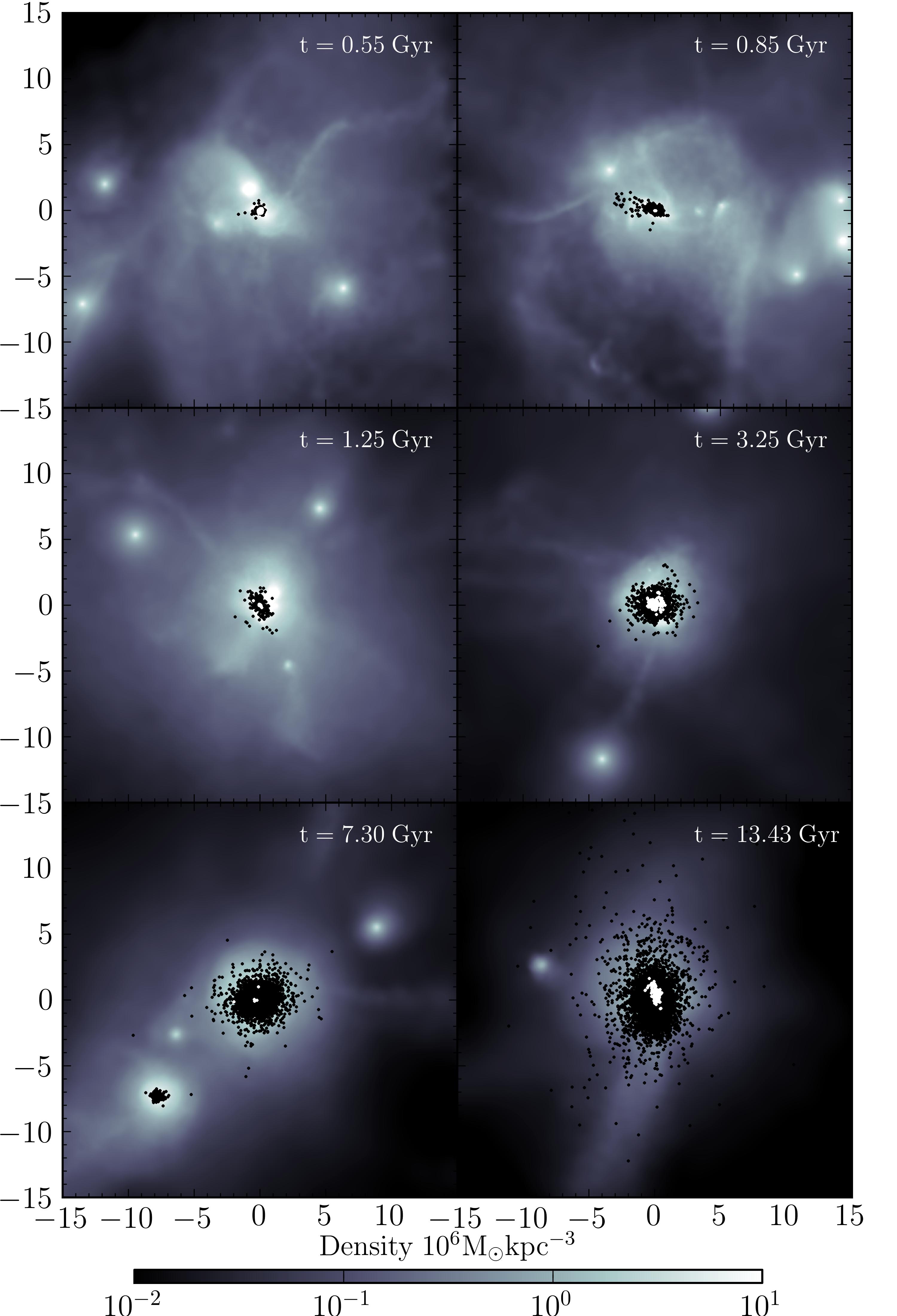
Figure 2: Snapshots of the merger simulation corresponding with tree MT4 from Fig. 1. The grayscale represents the gas density, the white dots show the young stars which are younger then 0.1 Gyr and the black dots show all the stars in the galaxy. In each panel the snapshot time is indicated, the $x$ and $y$-labels are in kpc.

3 Analysis

3.1 Star formation histories

In Fig. 3 and Fig. 4 the star-formation histories (SFHs) of different merger trees are shown, all with the same final halo mass of respectively 2.5$\times$10⁹ M_⊙ (Fig. 3) and 7.5$\times$10⁹ M_⊙ (Fig. 4). For comparison, the SFH of an isolated model with the same final halo mass is plotted in these figures.

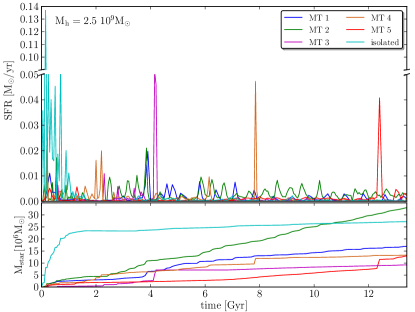
Figure 3: Top panel: the total SFR of several merger trees and a reference isolated simulation with the same final halo mass of 2.5$\times$10⁹ M_⊙ as a function of time. Bottom panel: the stellar mass as a function of time. (A color version of this figure is available in the online journal.)

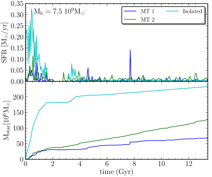
Figure 4: Identical as Fig. 3 but for a final halo mass of 7.5$\times$10⁹ M_⊙. (A color version of this figure is available in the online journal.)

3.1.1 Isolated galaxies

The isolated models form most of their stellar mass during the first 2 Gyr of the simulation after which star formation shuts down for approximately 2 Gyr due to the depletion of gas by SN feedback which prevents the gas density to reach the threshold for star formation. The star formation restarts around 4 Gyr when part of the gas has been able to return. After that, star formation can proceed in an episodic fashion, such as in the isolated model presented in Fig. 3, or as low-level residual star formation, as in the isolated model presented in Fig. 4. The major difference between the different mass models in isolation is the amplitude of the star formation, which increases with increasing mass.

3.1.2 Merged galaxies

In Figs. 3 and 4, the sum of the SFR of all the members of a merger tree is plotted. In the first two Gyrs of the simulation, it is difficult to disentangle the difference between star formation occurring naturally inside any given halo and star formation prompted by mergers. After this period, the peaks in the SFH can be shown to correspond to the major merger events in the merger trees. For example, in Fig. 3, we see a peak for MT3 around 4.25 Gyr in the simulations which corresponds with the major merger in MT3 around 4.57 Gyr in Fig. 1. Similarly, a peak in the SFH of MT4 is seen around 7.8 Gyr and in MT5 around 12.5 Gyr, these correspond respectively with a major merger around 7.35 Gyr for MT4 and around 13.75 Gyr for MT5. We see that these SF peaks are in close agreement with the desired merger history we wanted to generate. However, small deviations are possible and they are due to:

1. The 2-body approximation that is used to determine the orbital parameters. In the simulation multiple mergers will be possible.

2. The calculated merging time is the time to pericenter but the large peaks in the star formation will occur only when they actually merge.

As in binary merger studies (Di Matteo et al., 2007; Cox et al., 2006; Torrey et al., 2012; Scudder et al., 2012), we see that the peaks in the SFR occur at the end of the merging process of two galaxies. At the first pericenter passage their is a modest increase of the SFR due to tidal squeezing of the gas while a larger increase is noticeable when the galaxies really collide. For example in Fig. 3, showing the results for models with a final halo mass of M_h=2.5 10⁹ M_⊙, the small SF peaks at 3.65 Gyr of MT3 and at 6.2 Gyr at MT4 are created by the first pericenter passage of the halo before the large peak in SFR. There is no such first small peak for MT5 since the merger proceeds very rapidly. However, now the main star-formation peak is somewhat broadened. MT2, and to a lesser extent also MT1, lacks strong starbursts that would otherwise suppress subsequent star formation. Its minor mergers keep stirring up the gas and cause many small star-formation events. Its mass therefore gradually builds up and, in the case of MT2, eventually exceeds that of the isolated model.

We also see a double peak in the SFH for the more massive merger tree MT1 with final halo mass of M_h=7.5 10⁹ M_⊙ in Fig. 4 at 7.2 Gyr and 7.7 Gyr and a triple peak due to a merger with three components at 4.15 Gyr, 4.6 Gyr and 4.8 Gyr. MT2 in Fig. 4 has some major mergers very early on in the simulation but for the main part of its evolution it is has a continuously supply of gas by minor mergers.

Di Matteo et al. (2007) did a statistical study of binary interactions and mergers of galaxies of all morphologies from ellipticals to late type spirals. However, our sample is less numerous and contains less massive and less disky systems but we can check if we observe similar trends. To start with, a negative correlation was found for the peak star-formation rate and the strength of the tidal interaction between a galaxy pair at first pericenter passage. The latter can be quantified by the pericenter distance, $r_{p}$, the pericenter velocity, $v_{p}$, or the tidal parameter, $T_{p}$, defined as the sum of the tidal forces of each component each described by:

$$T_{p,i}=\log_{10}\Big{[}\frac{M_{comp}}{M_{i}}\Big{(}\frac{D_{i}}{r_{p}}\Big{)}^{3}\Big{]}\ \ i=1,2$$ (13)

with $M_{i}$ the mass of the galaxy, $M_{comp}$ the mass of the companion, $r_{p}$ the pericenter distance and $D_{i}$ the scalelength of the galaxy, calculated as the radius containing 75% of the dark matter mass. Although we of course have much less data to rely on, Table 2 shows a similar trend for the most massive major mergers of MT3, MT4 and MT5 of the models with final halo mass of M_h=2.5 10⁹ M_⊙, where we see that a decrease in pericenter distance corresponds to an increase in the amplitude of the SF peak. Similarly, an increase in the velocity at the pericenter, $v_{p}$, corresponds in the models with a decrease in SFR_peak in our data, although Di Matteo et al. (2007) found no correlation between these two parameters. However, our models have a similar trend as the models of Di Matteo et al. (2007) where an increase of SFR_peak occurs when the characteristic encounter time, $t_{enc}=\frac{r_{p}}{v_{p}}$ increases. The explanation for these trends provided by Di Matteo et al. (2007) is that a gentler first pericenter passage allows the orbiting galaxies to retain more of their gas for future consumption during the final merger phase.

Di Matteo et al. (2007) found a clear trend for galaxy pairs to have lower peak star formation rates when they merge if they experienced intense tidal forces at first pericenter passage. This is due to two effects. On the one hand, stronger tidal squeezing on the way to pericenter leads to a slightly enhanced gas consumption by star formation around pericenter passage while, on the other hand, stronger expansion of the outer parts of the system after pericenter passage induces a more significant loss of gas in tidal tails. We find a similar trend that galaxies which endure a strong tidal force during their first pericenter passage have lower SF peaks when they merge.

MT	$r_{p}$	$v_{p}$	$t_{enc}$	SFRpeak	$T_{p}$
	[kpc]	[km/sec]	[Myr]	[M⊙/yr]
MT3	2.36 kpc	40.5	56.9	0.051	5.40
MT4	0.91 kpc	141.3	6.3	0.049	6.71
MT5	0.12 kpc	398.9	0.29	0.040	9.53

Table 2: The properties of the most massive major mergers of MT3, MT4 and MT5 of the models with M_h=2.5 10⁹ M_⊙. The columns show (1) the pericenter distance, (2) the velocity at the pericenter, (3) the duration of the encounter, (4) the peak in the SF due to the merger, and (5) the tidal parameter.

Table 3 shows the final stellar mass of the different simulations. For the same halo mass, the merger simulations produce less stars than the isolated simulations. So, while mass is the main parameter determining the properties of isolated simulated galaxies, this is no longer true for the merger simulations. Mergers are able to fling large amounts of gas to large radii, where it is inaccessible for star formation and the merger history will determine when gas will be delivered to the center of a galaxy.

In addition, we can distinguish two extreme types of merger trees which reflect most clearly how the merger history influences a galaxy’s star formation history and final stellar mass. On the one hand, merger trees can have a massive progenitor present early on in the simulation which subsequently grows through minor mergers, such as MT1, MT2, and, to a lesser extent, MT4 (see Fig. 1). At the other extreme, there are merger trees with many low-mass progenitors that merge only late in cosmic history, such as MT3 and MT5. In the former, the massive progenitor is already relatively efficient at forming stars from the start of the simulation while subsequent minor mergers will fuel further star formation. This leads to a continuously increasing stellar mass. In the latter, the many low-mass progenitors are inefficient star formers and the stellar mass increases mostly during merger-induced bursts. The former type of merger tree also leads to galaxies with higher stellar masses at a given halo mass than the latter type. Of course, merger trees fill in the continuum between these two extreme types. For instance, MT4 has a merger tree that is intermediate between the two extreme cases.

Recently, observed SFHs, derived from color-magnitude diagrams, have become available for sizable samples of dwarf galaxies (Monelli et al., 2010b, a; Cole et al., 2007; Weisz et al., 2011; Hidalgo et al., 2011; McQuinn et al., 2010a, b). The time resolution of these SFHs can be as good as 10 Myr for the most recent epochs, deteriorating to over 500 Myr for stellar populations older than 1 Gyr. The SFHs derived by e.g. McQuinn et al. (2010a) for the last 1.5 Gyr are well resolved and show that the SFRs of dwarf galaxies can fluctuate strongly and erratically, with no discernible periodicity. These authors find that a burst produces between 3 and 26 % of the final stellar mass in the observed dwarfs. In our simulations, a starburst produces between 7 % and 29 % of the final stellar mass. A notable exception is the extreme, 6-fold merger in simulation MT3 with halo mass 2.5$\times$10⁹ M_⊙ at 4 Gyr, which produces 47 % of the stellar mass. The observed bursty dwarfs have SFRs that vary from 0.0003 M_⊙/year (Antlia) over 0.05 M_⊙/year (IC4682) up to 0.4 M_⊙/year (NGC5253). Our simulated dwarfs have mean SFRs of the order 0.005-0.01 M_⊙/year, comparable to e.g. UGC4483, NGC4163, UGC6458, and NGC6822. The observed ratio of the burst peak SFR to the mean SFR falls in the range $b\sim 3-14$. The simulated galaxies see peak increases of the order of $b\sim 10$ in the strongest starbursts and $b\sim 2$ in the weakest bursts.

In section 3.1.1 we already pointed out that the isolated non-rotating galaxy simulations often have episodic SFHs. The merger tree SFHs, on the other hand, are much more erratic and variable, without fixed periodicity, much like the SFHs of real dwarfs.

3.2 Scaling relations

Here we compare the gross properties of the simulated dwarfs, both with and without merger trees, with observed kinematic and photometric scaling relations at $z=0$. For the observational data: the data from De Rijcke et al. (2005) are converted from B-band to V-band using the relation: (B-V)=0.7. From the Graham & Guzmán (2003) paper we converted their B-band magnitudes into V-band magnitudes as described in De Rijcke et al. (2009) (using a B-V colour-magnitude relation constructed from the M_V-(V-I)-[Fe/H] relation in combination with SSP models for 10-Gyr-old stellar populations (from Vazdekis et al. (1996))). The LG data and the data from De Rijcke et al. (2009), Grebel, Gallagher & Harbeck (2003), Hunter & Elmegreen (2006), Dunn (2010) and Kirby et al. (2013) are presented in the V-band, so no transformation was needed. The V-band magnitudes of van Zee (2000) and van Zee, Barton & Skillman (2004) are deduced from their B-band magnitude and their B-V color. For the Antlia data from Smith Castelli 2008, the C-T₁ colours were (as in De Rijcke et al. (2009)) converted to the C-T1 colours using empirical (C-T₁)-[Fe/H] and [Fe/H]-(V-I)-relations. For the $\sigma$-L_B plot we need the data in B-band, which was available for all the data with the exception of Geha, Guhathakurta & van der Marel (2003) where we transform the V-band magnitude to the B-band magnitude using M_V=M_B-0.7. We present the dIrr, dSph and dE data in Fig. 5 using respectively black (magenta), light-grey (yellow) and dark-grey (green) dots.

3.2.1 Half-light radius R_e

In panel a.) of Fig. 5 the effective radius, $R_{e}$ is shown as a function of the V-band magnitude. The black hexagons represent the isolated simulations, where the increase in V-band magnitude follows the increase in final halo mass (from respectively 10⁹ M_⊙ to 10¹⁰ M_⊙). The merger simulations are indicated by different symbols/colors corresponding to different final halo masses. In Table 3, the value of the effective radius is given for each of the simulated models.

In the observational data, the effective radius increases with increasing V-band luminosity. The simulations have the same trend, but the slope of the merger simulations is steeper compared with the observational data with which the slope of the isolated models shows a better agreement. However, our isolated simulations are too compact while the merged galaxies are larger and more in agreement with observed dwarf galaxies.

The larger effective radius of dwarf galaxies with merger histories indicates that star formation is more widespread in these galaxies. One important factor in determining the size of a galaxy’s stellar body is the depth of its DM potential, as this influences the gravitational force on the gas. In the isolated models we already notice a conversion of the cusped NFW profile to a cored density profile due to baryonic processes (Cloet-Osselaer et al., 2012). In paragraph 4.1, we show that the flattening of the cusp is more pronounced in galaxies with a merger history. This may explain the difference in $R_{e}$ between simulated galaxies with and without merger histories in panel a.) of Fig. 5. Moreover, the difference between the isolated models and the merger models increases with halo mass. This may be due to the fact that the dark matter density distribution flattens more in more massive merger models.

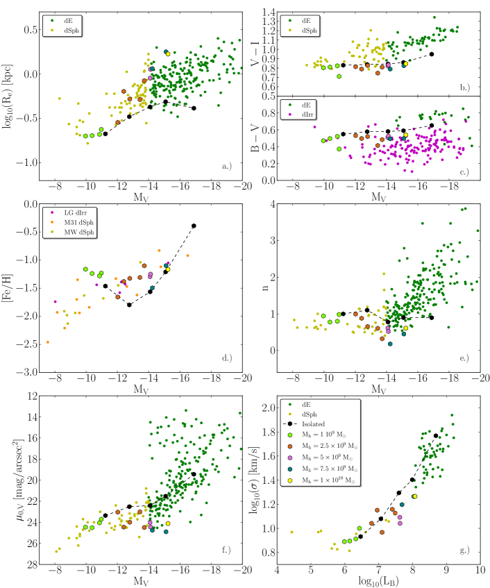
Figure 5: Some scaling relations and the surface brightness parameters as a function of the magnitude. In a.), the half-light radius $R_{\rm e}$ is plotted, in b.) and c.) the $V-I$ color and $B-V$ color is plotted, d.) shows the iron content [Fe/H]. In panel e.) and f.), the Sérsic index $n$ and central surface brightness $\mu_{0}$ are plotted and in g.) the Faber-Jackson (FJ) relation is plotted. All these quantities are plotted against the $V$-band magnitude, except the FJ relation which are plotted as a function of the $B$-band luminosity. The isolated models are plotted by connected black diamonds with increasing final halo mass. For the merger trees the models are represented by different symbols depending on the final dark matter mass as indicated by the legend. Our models are compared with observational data obtained from De Rijcke et al. (2005) (DR05, dEs), Graham & Guzmán (2003) (GG03, dEs), van Zee, Barton & Skillman (2004) (dEs), van Zee (2000) (dIrr), Hunter & Elmegreen (2006) (dIrr), LG data (dSphs) come from Peletier & Christodoulou (1993), Irwin & Hatzidimitriou (1995), Saviane, Held & Piotto (1996), Grebel, Gallagher & Harbeck (2003), McConnachie & Irwin (2006), McConnachie, Arimoto & Irwin (2007), Zucker, Kniazev & Bell (2007), Perseus data from De Rijcke et al. (2009) (dSphs/dEs), Antlia data from Smith Castelli et al. (2008) (dEs). For the [Fe/H]$-M_{V}$ plot, data from Kirby et al. (2013) was used for MW dSphs, M31 dSphs and Local Group dIrr. For the Faber-Jackson relation data from Geha, Guhathakurta & van der Marel (2003) (dEs), Kleyna et al. (2005) (dSphs), Mateo (1998) (dEs/dSphs), Peterson & Caldwell (1993) (dEs), van Zee, Barton & Skillman (2004) (dEs) and De Rijcke et al. (2005) (dEs) is used. The dIrr, dSph and dE are shown by dots in different colors, respectively black (magenta), light-grey (yellow) and dark-grey (green) . (A color version of this figure is available in the online journal).

Table 3: Final properties of our simulations. The different blocks represent different final halo. Columns: (1) model type, (2) the final stellar mass in units of 10⁶ M_⊙, (3) V-I color, (4) mass-weighted metallicity, (5) the Sérsic index. (6) the mean surface brightness within the half-light radius, (7) the central one dimensional velocity dispersion, (8) the logarithm of the final specific stellar angular momentum, (9) the ellipticity, (10) the ratio of the maximal stellar velocity divided by the central one dimensional velocity of the galaxy and of a isotropic rotator, (11) and (12) respectively the amount of major and minor mergers in the formation histories, where we consider minor mergers to have mass ratios greater than 1:3.

$\mathrm{model}$	$M_{\rm\star,f}$	$R_{\rm e}$	$V-I$	$[Fe/H]$	$n$	$\mu_{0,V}$	$\sigma_{\rm 1D,c}$	$\log{j_{\star,f}}$	$e$	$(V/\sigma)^{\star}$	$\#~{}MM$	$\#~{}mM$
	$[10^{6}\ M_{\odot}]$	$[kpc]$				$[mag]$	$[km/s]$	$[km~{}sec^{-1}~{}kpc]$
$\mathrm{M_{h}=1\times 10^{9}\ M_{\odot}}$
Isol	5.61	0.21	0.83	-1.46	1.00	22.81	8.54	-0.29	0.26	0.57	0	0
MT 1	1.36	0.24	0.71	-1.23	0.98	23.71	10.01	0.25	0.42	1.12	4	5
MT 2	2.71	0.21	0.82	-1.28	0.80	24.05	8.18	-0.74	0.11	0.36	3	8
MT 3	1.25	0.20	0.81	-1.24	0.78	24.51	7.85	-0.35	0.32	0.59	6	9
MT 4	0.79	0.20	0.80	-1.16	0.94	24.46	7.76	-0.39	0.34	0.53	4	12
$\mathrm{M_{h}=2.5\times 10^{9}\ M_{\odot}}$
Isol	27.22	0.33	0.84	-1.80	1.10	21.94	11.99	0.57	0.12	2.05	0	0
MT 1	16.97	0.52	0.83	-1.33	0.66	23.99	9.27	0.64	0.20	1.46	4	8
MT 2	33.13	0.84	0.81	-1.10	0.32	24.49	13.39	1.03	0.22	1.89	3	7
MT 3	9.22	0.29	0.81	-1.66	0.99	23.04	11.00	0.24	0.16	0.56	11	8
MT 4	13.40	0.64	0.79	-1.38	0.88	24.46	14.14	0.39	0.43	0.26	4	13
MT 5	12.97	0.52	0.75	-1.31	0.60	23.01	14.39	0.42	0.11	0.52	6	8
$\mathrm{M_{h}=5\times 10^{9}\ M_{\odot}}$
Isol	94.86	0.43	0.84	-1.56	0.77	21.82	19.69	0.69	0.22	1.14	0	0
MT 1	55.50	0.90	0.82	-1.30	0.61	24.03	12.35	0.49	0.06	0.50	7	12
MT 2	65.50	1.13	0.83	-1.25	0.52	24.45	11.00	0.11	0.31	0.19	5	17
$\mathrm{M_{h}=7.5\times 10^{9}\ M_{\odot}}$
Isol	233.56	0.49	0.86	-1.21	0.90	20.93	25.33	0.71	0.10	1.23	0	0
MT 1	68.70	1.15	0.79	-1.50	0.18	24.75	15.73	1.02	0.26	0.40	12	8
MT 2	127.58	1.78	0.82	-1.10	0.45	24.90	18.38	1.42	0.21	0.86	5	15
$\mathrm{M_{h}=1\times 10^{10}\ M_{\odot}}$
Isol	1288.10	0.41	0.95	-0.39	0.89	18.79	58.69	0.40	0.16	0.17	0	0
MT 1	178.56	1.68	0.85	-1.17	0.61	24.12	18.42	1.31	0.47	0.45	5	7

3.2.2 The V$-$I and B$-$V color.

The V$-$I and B$-$V color as a function of the V-band magnitude is shown in respectively panel b) and c) of Fig. 5. The V$-$I color has a value significantly below V$-$I$\sim 0.7$ mag only in stellar populations with ages below a few 100 Myr. We see that the V$-$I color is constant around a value of $\sim 0.8$ mag for the entire magnitude range with a scatter of 0.05 mag. There are some galaxies which, due to a late star formation burst, have smaller values for V$-$I. For example, MT5 from Fig. 3 has the lowest V$-$I value in its mass range (see Table 3), due to a recent peak in star formation at 12.4 Gyr. The other MTs have similar values for their V$-$I color which is due either to a similar late SF peak or by continuous star formation at a small rate. Likewise, the B$-$V color scatters within 0.1 mag around a value of $\sim 0.5$ mag for the entire luminosity range.

In terms of the V$-$I color, the simulations are significantly bluer than dSphs and dEs, with the merger simulations slightly bluer than the isolated simulations. In terms of the B$-$V color, the simulations are comparable to observed dIrrs, although on the red side of the dIrr color distribution.

This is caused by the larger gas fraction of the simulated dwarfs since there are no environmental effects present that could remove gas. As a result, low level star formation occurs during the last 6 Gyr of the simulations generating young, blue stars. The isolated galaxies are generally redder as most of their stars have been formed early on in the simulation. Overall, very different SFHs due to different merger histories all result in approximately the same V$-$I and B$-$V color.

Our rather blue models, which are more in agreement with observed dIrr due to their large gas content and ongoing star formation, could be transformed into red and dead dSph by external interventions which remove the gas and shut down star formation for the last Gyr of the simulation. Examples of such external processes are: ram-pressure stripping (Mayer et al., 2006; Boselli et al., 2008), tidal interactions (Mayer et al., 2001b, a), and the UV background (Shaviv & Dekel, 2003). However, for the simulations presented here we did not implement such external processes, so star formation continues till $z=0$ and the simulated galaxies are bluer than the observed dSph/dE galaxies. and more in agreement with the observed dIrrs which are caracterized by ongoing star formation.

Incorporating gas depleting processes, such as gas stripping and the cosmic UV background, in the simulation code is currently ongoing, using the cooling and heating curves from De Rijcke et al. (2013) which contain the UVB.

3.2.3 The metallicity

Panel d) in Fig 5 shows the luminosity weighted Iron abundance, [Fe/H], a tracer of the metallicity of the stars, as a function of the V-band magnitude. The simulations are compared with observational data from Kirby et al. (2013) for Local Group dIrr (black/magenta dots), M31 dSph (light-grey stars/orange dots), and Milky Way dSph (ligth-grey/yellow dots).

With increasing mass, the isolated simulations tend to become too compact leading to fast and self-enriching star formation. This causes the bright side of their M_V-[Fe/H] relation to be too steep. For the least massive merger models, with halo masses around 10⁹ M_⊙, the metallicity is too high by about 0.4 dex compared with the observational data. This is because only near the galaxy center does the gas density exceed the density threshold for star formation. This centrally concentrated star formation then self-enriches too much. Star formation is centrally concentrated in the least massive isolated model as well but in this case a significant fraction of the stars form early on from almost unenriched gas, causing the mean metallicity to be lower than in the merger models.

The metallicities of the more massive merger models are in better agreement with the observations. In the latter, star formation occurs spatially more widespread and self-enriches less. Except for the least massive ones, the metallicities of the merger simulations compare well with those of the observed Local Group dwarfs.

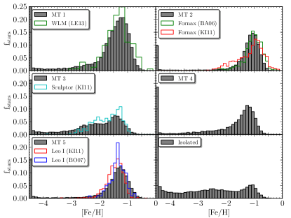
Figure 6: A histogram of the metallicity distribution of the stars. The simulations all produce dwarf galaxies with final halo mass of 2.5$\times$10⁹ M_⊙. The simulations are compared with observational data from Battaglia et al. (2006) (BA06), Kirby et al. (2011) (KI11) and Bosler, Smecker-Hane & Stetson (2007) (BO07). (A color version of this figure is available in the online journal.)

In Fig. 6, the metallicity distribution function (MDF) of the different merger trees and the isolated simulations at $z=0$ is plotted in a histogram. As explained in paragraph 2.1, the gas already has a very small metallicity ($Z=10^{-4}\ Z_{\odot}$) from the start of the simulation. All stars formed from this gas will have exactly the same Iron abundance of [Fe/H]$=-4.45$, causing a spike in the MDF at this metallicity. This is an artefact of our idealised initial conditions.

The isolated simulated galaxies generally have a larger fraction of metal-poor stars than galaxies with a merger history. This is due to the first, large star formation peak consuming the metal-poor gas reservoir in isolated simulated galaxies. In merger simulations, the interaction induced star formation rapidly boosts the metallicity to [Fe/H]$\sim-1$, thus suppressing the low-metallicity tail. One notable exception is MT3 whose merger tree contains relatively few mergers during the first 3 Gyr. Star formation in its isolated progenitor galaxies produces a population of low-metallicity stars, peaking in the metallicity range [Fe/H]$\sim-3$ to $-2$.

As an illustration, we compare the MDFs of some of the merger tree simulations with those of observed Local Group dwarf galaxies: Fornax, Sculptor, Leo I and WLM. With absolute magnitudes of, respectively, M${}_{V}=-13.3$ mag, $-11.1$ mag, $-11.8$ mag and $-14.92$ mag (Irwin & Hatzidimitriou, 1995; Mateo, 1998; Łokas, 2009; de Vaucouleurs et al., 1991) these galaxies fall in the luminosity interval covered by the simulations. Each galaxy is compared with a merger tree simulation that closely matches its mean [Fe/H]: [Fe/H]=-0.99, -1.68, and -1.43 for Fornax, Sculptor, and Leo I (Kirby et al., 2011) and WLM with  [Fe/H]=-1.28 (Leaman et al., 2013), respectively, and [Fe/H]=-1.1, -1.66, -1.31, and -1.33 for MT2, MT3, MT5, and MT1 respectively. All MDFs, simulated and observed, are normalized to unity over the metallicity interval from [Fe/H]=-4 to [Fe/H]=0. The Fornax MDFs are taken from Battaglia et al. (2006) (BA06) and Kirby et al. (2011) (KI11), those of Sculptor from KI11, those of Leo I from KI11 and from Bosler, Smecker-Hane & Stetson (2007) (BO07) and the WLM MDF is taken from Leaman et al. (2013). Clearly, there can be a significant author-to-author difference between observed MDFs of the same galaxy. This could be caused by the different number of stars included in the samples and by the different spatial extents covered by the observations, if the stellar populations are spatially segregated.

The low-metallicity tail of the Fornax data of BA06 was explained to originate from the infall of a metal poor component based on its non-equilibrium kinematics and radial metallicity gradient. The analysis of KI11 suggested Fornax to have an extended SFH due to the metal-rich peak in the MDF which is caused by star formation from previously enriched gas. As MT2 already has a massive component containing roughly half of its final mass at one Gyr in the simulation after which it receives metal-poor gas from multiple minor mergers triggering SF, this explains why the simulation is most in line with the results of KI11. The same is true for the MDFs of MT1 and MT4.

Like MT3, Sculptor has a bimodal MDF with a high-metallicity peak around [Fe/H]$\sim-1.3$ and a low-metallicity peak below [Fe/H]$\sim-2$. We merely wish to illustrate that such bimodal MDFs are also found among real dwarfs in this luminosity range. Moreover, the agreement is not perfect: MT3 contains more low-metallicity stars than Sculptor and the high-metallicity peak is less strong.

We can conclude from Fig. 6 that the peaked MDFs of the merger-tree simulations are much more in agreement with the observations than the flat MDFs of the isolated models.

3.2.4 The Sérsic parameters

Panels e) and f) show in Fig. 5 show respectively the Sérsic index $n$ and the central surface brightness in the V-band, $\mu_{0,V}$. In both cases the simulations are compared to observational data of dE/dSph galaxies. Generally, for all mass models and different merger trees, the models overlap with the Sérsic parameter data in the regime of the dwarf spheroidals. The scatter in the simulations is mainly due to the different merger histories.

Sérsic index, $n$

The merger simulations have similar $n$-values as the observational data and are smaller or equal compared to the Sérsic indices of isolated simulations. We see that neither the merger tree, nor the flattening of the central core has a significant influence on the Sérsic index of the simulations.

Central surface brightness in the V-band, $\mu_{0,V}$

The isolated models follow the trend of increasing central surface brightness with increasing V-band magnitude. The most massive merger simulations have lower central surface brightnesses compared to the isolated models but are still in agreement with the observations. This low $\mu_{0,V}$-value is due to the flatter DM core which causes star formation to occur less centrally and results in a more extended, less dense stellar body.

3.2.5 The Faber-Jackson relation

After the photometric relations, we now turn to the kinematic relations, where panel g.) of Fig. 5 shows the velocity dispersion of the stars as a function of the B-band luminosity. Our simulations follow the same trend as the observational data. The isolated simulations have velocity dispersions which are somewhat large compared to the observations. The merger simulations are better in agreement with the observations but they show some spread which is due to the different merger histories which result in different flattenings of the dark matter core.

For more massive haloes, the velocity dispersion of the merged galaxies deviates markedly from that of the isolated galaxies. Again, this is most likely due to the stronger flattening of the dark matter halo in more massive galaxies, see section 4.1. Due to the lower central density and the shallower potential, stellar velocities will be lower, resulting in a lower velocity dispersion.

4 Discussion

4.1 The dark matter halo

Figure 7: The dark matter distribution of a halo with mass 2.5$\times$10⁹ M_⊙ at $z$=0. The units on the the box are in kpc.

Figure 8: The dark matter distribution of a halo with mass 7.5$\times$10⁹ M_⊙ at $z$=0. The units of the box are in kpc.

In order to create dark-matter density profiles, the isolated simulations are centered on the center of mass of the dark matter haloes. For the merger simulations, this approach is less obvious since the merging process of the dark matter haloes produces tidal tails which extend to large radii. As a result, the center of mass of a halo can deviate significantly from what one would consider “by eye” to be the location of the center of the main halo. Moreover, as can be seen in Fig. 7 and Fig. 8, the dark-matter haloes of galaxies with a merger history contain substantial substructure until the end of the simulation. So, to find the center of the main halo, a 3D Voronoi tessellation (Schaap & van de Weygaert, 2000) is used to determine the density at the position of each dark matter particle. The 15 particles with the highest densities are then selected. Finally, the center of the halo is equated to that particle out of those 15 which has the largest mass within a 2 kpc sphere in order to avoid local density peaks. A visual check proved that this procedure yields a meaningful estimate for the halo center. The dark-matter density profile is derived from the mass enclosed inside increasingly large spherical shells centered on the halo center identified as explained above.

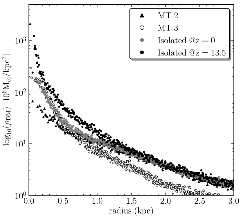
Figure 9: The dark matter density profile of the merger simulations MT2 and MT3 at $z=0$ and one isolated galaxy with a final halo mass of 2.5$\times$10⁹ M_⊙ at $z=0$ and $z=13.5$.

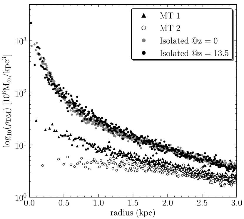
Figure 10: The dark matter density profile of the merger simulations at $z=0$ and one isolated galaxy with a final halo mass of 7.5$\times$10⁹ M_⊙ at $z=0$ and $z=13.5$.

In Figs. 9 and 10, the density profiles of the merged haloes with halo mass of respectively 2.5$\times$10⁹ M_⊙ and 7.5$\times$10⁹ M_⊙ are plotted at $z=0$ together with the density profiles of an equally massive isolated galaxy at $z=0$ and $z=13.5$. Very often, we see a conversion from a cusped NFW-profile (black dots) to a cored, or at least less steep, density profile (light-grey (cyan) dots) in the isolated galaxy simulations due to the effects of stellar feedback (Cloet-Osselaer et al., 2012). Haloes of galaxies with a merger history appear to become even shallower by $z=0$ than the isolated ones. Comparing the dark-matter density profiles in Figs. 9 and 10 with the merger trees that produced them (see e.g. Fig. 1) and the corresponding star-formation histories (see e.g. Figs 3 and 4) shows that the former is a non-trivial function of the merger history and the baryonic processes. The absorption of the orbital energy involved in a major merger will tend to inflate the dark-matter halo, causing the cusp to weaken. If a merger causes a rapid inflow of gas, it may compress the cusp whereas gas expulsion by supernovae may weaken the cusp.

In Fig. 11 and Fig. 12 the evolution of the inner slope of the dark-matter density profile, denoted by $\gamma$, is plotted for respectively MT2 and MT3 of the merger models with final halo mass of M_h,f=2.5$\times$10⁹M_⊙. $\gamma$ is determined by a least-square fit of a Nuker law (Lauer et al., 1995) to the density profile:

$$\rho(r)=\frac{\rho_{s}}{r^{\gamma}(r^{\beta}+r_{s}^{\beta})^{\alpha}}.$$ (14)

This function corresponds with a broken power-law function, where the break radius is described by $r_{s}$ and the sharpness of the transition is set by $\beta$. $\gamma$ represents the slope in the inner part, e.g. for $r\ll r_{s}$, $\rho(r)\sim r^{-\gamma}$, and $\alpha$ determines the outer power law as for $r\gg r_{s}$ $\rho(r)\sim r^{-\alpha\beta-\gamma}$. The NFW profile corresponds to $\gamma=1$, $\beta=1$, and $\alpha=2$. We omit the inner 60 pc from the fit; this corresponds to twice the gravitational softening length.

MT2 is a merger tree which already starts with a quite massive halo at early times, e.g. $\sim$53% of the final halo mass is present in the main halo after one Gyr in the simulation and the halo grows by the subsequent addition of minor mergers, each containing $\sim$1%-10% of the final halo mass. In Fig. 11, one first notices the adiabatic contraction of the halo, signaled by an increase of $\gamma$ to values above 1, due to the initial collapse of gas in the dark-matter potential well. Afterwards, the slope gradually decreases again due to the rapid removal of gas from the inner regions during repeated small starbursts triggered by the many minor merger events. MT1 and MT4 show a similar behaviour as MT2 in this regard.

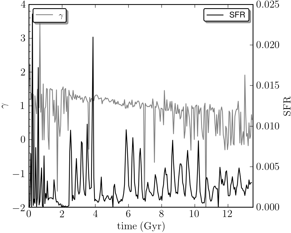
Figure 11: The evolution of the slope of the most massive component of MT2 in grey. The SFR is plotted by the black line.

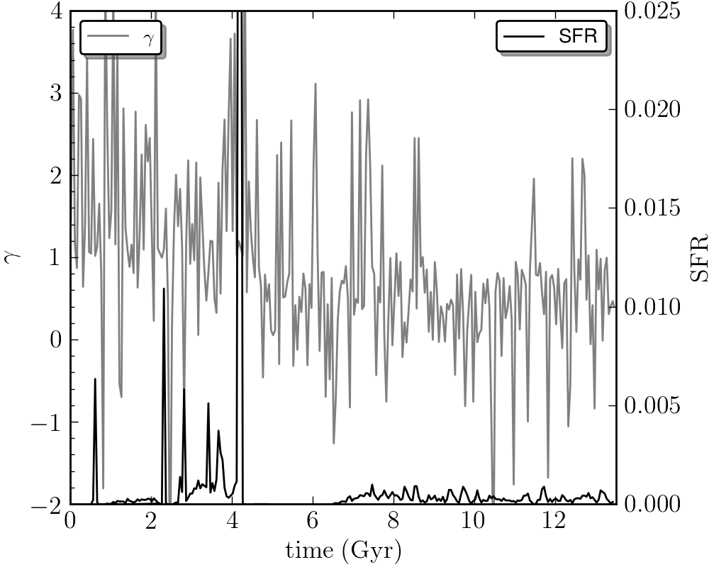
Figure 12: The evolution of the slope of the most massive component of MT3 in grey. The SFR is plotted by the black line.

MT3, on the other hand, is a merger tree where the mass builds up slowly over time, e.g. only $\sim$33% of the final halo mass is present in the main halo after one Gyr. Here, we trace the evolution of the slope $\gamma$ in the most massive halo present at each point of time in the tree MT3. A major merger occurs at 4 Gyr resulting in a large star formation peak and a subsequent shutdown of star formation. As shown in Fig. 12, the slope initially rapidly increases above 1, as in MT2. In this case, however, star formation is very low powered and the dark-matter cusp appears quite resilient against any small-scale gas motions. Only after the steep increase of the star-formation rate and the feedback activity connected with the major merger around 4 Gyr does the slope drop below $\gamma=1$. The starburst is actually so strong that star formation is halted for the next 1.5 Gyr and, when restarted, remains very weak and unable to further affect the dark-matter profile. In this case, the inner dark-matter slope remains stable. The dark-matter density profile of MT5 behaves similarly to that of MT3.

As shown in the literature, baryonic processes can explain the discrepancy between the cored dark matter density profiles of observed galaxies and the cusped dark matter density profiles deduced from cosmological simulations. First, the rapid removal of gas due to stellar feedback results in a non-adiabatically response of the dark matter halo and introduces a flattening of the cusped dark matter halo (Navarro, Eke & Frenk, 1996; Read & Gilmore, 2005; Mashchenko, Couchman & Wadsley, 2006; Governato et al., 2010; Pontzen & Governato, 2012; Governato et al., 2012; Cloet-Osselaer et al., 2012; Brooks & Zolotov, 2014). Secondly, the transfer of energy and/or angular momentum to the dark matter by infalling objects can transfer the cusped inner dark matter density profile into a more cored profile (Goerdt et al., 2006, 2010; Cole, Dehnen & Wilkinson, 2011). Repeated minor mergers can trigger small starbursts that rapidly evacuate gas from the galaxy center, with each burst slightly lowering the slope of the dark-matter density profile. Strong starbursts caused by major mergers have the same effect but, during star-formation lulls, the dark-matter density profile remains stable.

Merger trees with more massive final haloes show the same behavior, although Fig. 10, which shows the density profiles of haloes with final mass $M=7.5\times 10^{9}$ M_⊙, suggests that the flattening effect is much more pronounced for higher masses. This is likely caused by the stronger fluctuations in the star-formation rate (see Fig. 4) and by the fact that more massive merging galaxies need to absorb more orbital kinetic energy. Tree MT2 in this mass series of simulations contains a massive progenitor already early on which grows mainly through minor mergers. Star formation continues throughout the simulation, constantly reducing the inner dark-matter slope. MT1 contains major mergers that stop star formation for considerable timespans, limiting the flattening of the dark-matter cusp.

We conclude that the dark matter haloes are strongly influenced by the merger history and the resulting baryonic processes. Oh et al. (2011b) determined the inner density slopes within the central kiloparsec of the THINGS dwarf galaxies. They define the inner density slope $\alpha$ from a fit to the density profile $\rho\propto 1/r^{\alpha}$ and concluded a value of $\alpha=0.29\pm 0.07$ for the THINGS dwarf galaxies sample. In Oh et al. (2011a), the inner density profiles of simulated dwarf galaxies in a cosmological simulation were reported to have a slope of $\alpha=0.4\pm 0.1$. Here, we find, for instance, that for the inner dark-matter density slope of the haloes with final mass $M=2.5\times 10^{9}$ M_⊙ $\alpha=0.56\pm 0.27$. In order to explain the different slopes of the equally massive dark matter haloes, we have shown that small star formation peaks, due to repeated minor mergers, are efficient at lowering the slope. Major mergers cause a spike in the star-formation rate but feedback rapidly shuts down star formation, thus limiting the effect on the inner dark-matter density profile slope. This effect happens over all the full mass range but is more pronounced in the more massive models. The resulting shallow gravitational potential probably explains the large effective radii (see subsection 3.2.1) and low central velocity dispersions (see subsection 3.2.5) observed in some of the simulated galaxies.

4.2 Stellar specific angular momentum

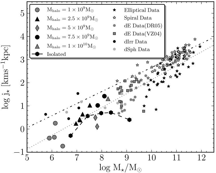
Figure 13: The stellar specific angular momentum at the end of the simulations ($z=0$) as a function of the stellar mass. Observational data of elliptical galaxies and spiral galaxies are taken from Romanowsky & Fall (2012) and a fit to the datapoints is plotted by a respectively the dotted and dash-dotted line. dE data of De Rijcke et al. (2005)(DR05) and van Zee, Barton & Skillman (2004)(VZ04) are plotted next to dIrr data and dSph data from Leaman et al. (2012), Kirby, Cohen & Bellazzini (2012), Kirby et al. (2014), McConnachie (2012), De Rijcke et al. (2006), McConnachie & Irwin (2006), Worthey et al. (2004), and Hidalgo et al. (2013).

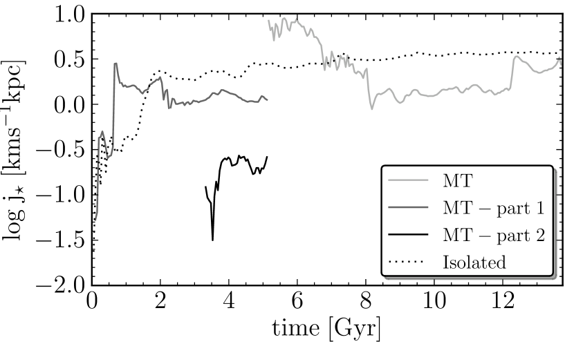
Figure 14: The evolution of the stellar specific angular momentum in time for an isolated simulation (dotted line) and for the merger simulation MT4, both with M_h,f=2.5$\times$10⁹M_⊙ (black, dark-grey and light-grey line).

Fig. 13 shows the specific angular momentum of the stars, $j_{\star}$, calculated as the length of the vector sum of the angular momenta of all the stars, using the center of mass of the most massive stellar body as a reference point, divided by the total stellar mass, as a function of the stellar mass, $M_{\star}$, at $z=0$. The isolated simulations are represented by connected black hexagons, with increasing stellar mass corresponding to increasing halo mass. The merger simulations, shown as indicated by the legend, represent different final masses of the dark matter halo. For comparison, observational data are also plotted. The data of the spiral and elliptical galaxies are taken from Romanowsky & Fall (2012), the observational data of dE from De Rijcke et al. (2005)(DR05) and van Zee, Barton & Skillman (2004)(VZ04) and data for dIrr and dSph are taken from Worthey et al. (2004), De Rijcke et al. (2006), McConnachie & Irwin (2006), Leaman et al. (2012), Kirby, Cohen & Bellazzini (2012), McConnachie (2012), Hidalgo et al. (2013), and Kirby et al. (2014). The simulations have similar specific angular momentum as the observed dwarf galaxies.

Like the observed galaxies, the simulated galaxies follow a trend of increasing stellar specific angular momentum with increasing stellar mass. At a given halo mass, the scatter on $j_{\star}$, caused by the different merger histories and star-formation histories, can be as large as an order of magnitude. In particular, merger histories that involve many mergers tend to produce galaxies with small $j_{\star}$ since the angular momenta of these mergers can cancel each other. Merger trees that involve few mergers have less opportunities for canceling orbital angular momenta and can produce galaxies with high $j_{\star}$.

In Fig. 14 the evolution of the stellar specific angular momentum is shown for an isolated simulation (dotted line) and a merger simulation (black, dark-grey and light-grey line), both with a final halo mass of 2.5$\times$10⁹ M_⊙.

Isolated galaxies

The stochastic nature of star formation is responsible for most of the stellar angular momentum that is created during the first Gyr of the simulation as stars are not created in a perfectly spherically symmetric way. In Fig. 14, the black line shows the evolution of the stellar specific angular momentum of an isolated galaxy. During the first Gyr, a large increase in stellar specific angular momentum occurs due to a large star formation peak. In the next Gyr, stars are mainly born out of the turbulent ISM. As the stars inherit the kinematics of the gas particles they are born from, the specific stellar angular momentum will increase. In addition, SNIa feedback asymmetrically accelerates the gas and, as a reaction, affects the stellar motions, increasing the specific stellar angular momentum.

Merged galaxies

The evolution of the stellar specific angular momentum for a merger simulation is plotted in Fig. 14. Around 5 Gyr into the simulation, two branches of the merger tree, represented by the black and dark-grey line, are put together. The joint system continues as indicated by the light-grey line. The large increase of $j_{\star}$ is the result of the vector sum of both the initial $j_{\star}$s of the branches, together with their orbital angular momentum. The incoming galaxy passes by the main galaxy at $\sim$6.4 Gyrs and starts to return to the main galaxy at $\sim$6.8 Gyr. At 7.8 Gyr it actually merges with the main galaxy, causing a large peak in the star formation rate (see Fig. 3). As the SF is centrally concentrated, it will not change the angular momentum much but the stellar mass will increase, resulting in a net decrease of the specific angular momentum. The same happens during the first two SF peaks of MT4 (see Fig. 3) at 2 and 2.2 Gyr which correspond to two decreases in $j_{\star}$ in the dark-grey curve in Fig. 14. For this specific merger, the net increase of the angular momentum is matched by the increase in stellar mass, producing only a small change of $j_{\star}$.

Around 12.3 Gyr there is another flyby of a galaxy which was thus far unable to form stars. When this galaxy enters the dense environment of the main galaxy it starts to form stars. After passing by the main galaxy, it keeps forming stars resulting in an increase of $j_{\star}$, due to more off-center star formation.

Mergers involving small halos incapable of forming stars or of triggering a star-formation event when captured influence the stellar specific angular momentum in a more indirect way: their angular momentum is absorbed by the main halo and can later be transferred to newborn stars.

From Fig. 13 we conclude that the merger simulations follow the observational trend, e.g. it is in line with the dotted trendline of the elliptical galaxies, which tend to have a lower specific angular momentum than spiral galaxies at a given stellar mass. This is a consequence of the fact that, depending on the orbits of the mergers, their mass ratio, their number, etc., the specific angular momentum can be higher in more massive galaxies. In other words: a galaxy that formed through a high orbital angular momentum, late, almost equal-mass merger will end up with a high stellar specific angular momentum.

4.3 Kinematics

4.3.1 Anisotropy diagram

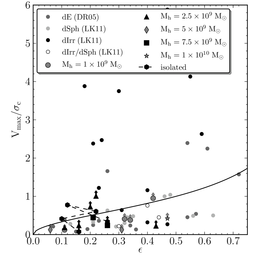
Figure 15: $(V_{max}/\sigma_{c})$, the ratio of the maximal rotation velocity of the stars and the central velocity dispersion of the stars as a function of the ellipticity. The simulations at $z=0$ are plotted together with dE data from De Rijcke et al. (2005), and dSph and dIrr data from Łokas, Kazantzidis & Mayer (2011). The black solid line shows the $(V/\sigma)$ relation for an oblate isotropic rotator. The arrows indicate that the estimation of V_max should be considered as a lower limit.

The ratio of the maximum rotational velocity of the stars, $V_{max}$, and the central velocity dispersion of the stars, $\sigma_{c}$, is plotted in Fig. 15 as a function of the ellipticity $\varepsilon=1-\frac{b}{a}$, with $b$ and $a$ the isophotal minor and major axis, respectively. To determine the flattening, the simulated galaxy is first rotated to align the $z$-axis with its rotation axis. Next, the density is evaluated at the effective radius in the equatorial plane, this isophote’s major axis $a$. Subsequently, the location along the $z$-axis is determined where the same density is reached, this isophote’s minor axis $b$. From this, the ellipticity of this isophote immediately follows. The maximum velocity is determined as the maximum of the least-square fitted function of the following form to the rotation velocity curve Giovanelli & Haynes (2002):

$$V(r)=a(1-e^{-r/b})\left(1+c\frac{r}{b}\right).$$ (15)

In some cases the rotation curve keeps increasing up to the last data point and the V_max-value should be considered as a lower limit. The fitted range that was used depends on the size of the galaxy and was chosen to be around 5 times the effective radius which is in agreement with the ’best range’ suggested by Romanowsky & Fall (2012), between 3 and 6 R_e, to calculate the rotation velocity for j_⋆-estimates.

Figure 16: The rotation velocity profile and a histogram of the distribution of stars as a function of radius. The dots represent the data of respectively the isolated model in black and of MT1 in gray and the line is the fit to the data. The dotted line indicates the location of 5$R_{e}$ and the dashed line shows the location of V_max.

Fig. 16 shows an example of the determination of V_max: the rotational velocity profile of an isolated simulation and of a merger simulation, respectively in black and gray. To each profile a fit is made and for the isolated simulation this reaches a maximum while for the merger simulations the fit keep increasing so V_max is taken to be the value at 5$R_{e}$. The location of 5$R_{e}$ is indicated by the dotted line while the value of V_max is shown by the dashed line. The histogram shows the distribution of the stars. In the isolated simulation the stars are more centrally concentrated and most of the angular momenta is located at large radii. In the merger simulations, the stellar body extends much further compared to the isolated simulation.

Most of the simulations are located below the relation for oblate isotropic rotators defined as $(V/\sigma)_{theo}=\sqrt{\varepsilon/(1-\varepsilon)}$ and indicated by the black line in Fig. 15. This shows that velocity anisotropy plays a substantial role in stabilizing them. In Table 3, the value $(V/\sigma)^{\star}$ is shown for the simulations, this is the ratio of $V_{max}/\sigma_{c}$ and the theoretical value for an isotropic oblate rotator. Hence, a $(V/\sigma)^{\star}$-value of one corresponds to an isotropic oblate rotator. Most merger simulations have $(V/\sigma)^{\star}$ values lower then 1. Some of the isolated simulations have $(V/\sigma)^{\star}$-values much larger than one. However, their maximum rotation velocity is reached by stars at the outskirts of the stellar body, beyond $\sim 5$ half-light radii. Therefore, for these galaxies, no relation between $V_{max}/\sigma_{c}$ and the stellar body’s ellipticity is expected.

Cox et al. (2006) found that dissipationless and dissipational (with a gas fraction of 0.4) binary mergers remnants are located in different locations in the anisotropy diagram, with the former having much lower $(V/\sigma)^{\star}$-values than the latter. The location of the merger simulations agrees with the dissipational binary merger remnants of Cox et al. (2006), which could be expected as our simulations are all gas rich mergers. The merger simulations cover a wider range in ellipticities, between 0.06 and 0.47, compared to the isolated models which have ellipticities between 0.10 and 0.26 indicating that the merger events are efficient in creating flattened galaxies. However, there is no clear connection between the characteristics of the merger tree and the final ellipticity. For example, the merger simulations with a final halo mass of 7.5$\times$10⁹ M_⊙ have very different merger histories but have almost identical final ellipticities.

4.3.2 Shapes - Triaxiality

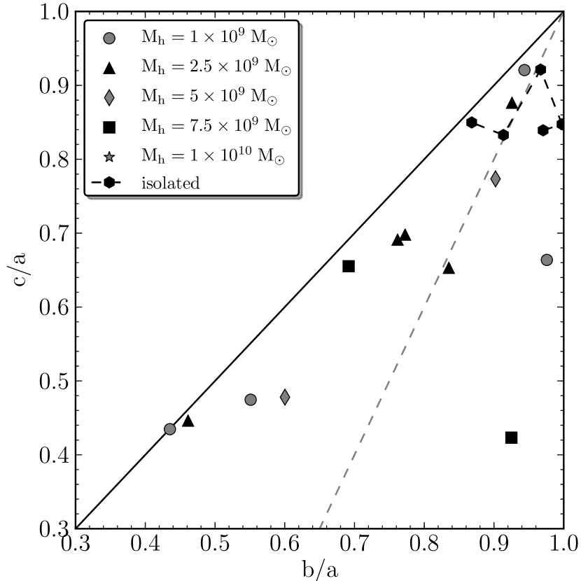
Figure 17: The shape diagram where the axis ratio b/a is plotted as a function of $c/a$ with $c<b<a$. The black line corresponds with prolate spheroids which for which $b=c$ while oblate spheroids are located near the $b/a=1$ line. The dashed line corresponds to the models with maximum triaxiality.

In Fig. 17, the shape diagram of the simulated galaxies is plotted. Each galaxy has first been aligned with the principal axes of its inertia tensor (Franx, Illingworth & de Zeeuw, 1991; González-García & van Albada, 2005; Cox et al., 2006). The order of the three axes is determined from the density profile along each axis, with $c<b<a$. Then, the two axis ratios $c/a$ and $b/a$ are measured similarly to the flattening $\varepsilon$ in the previous paragraph: the density is evaluated at the effective radius along the longest axis and those positions along the shortest and intermediate axes are determined where the same density is reached. Oblate spheroids have $b/a=1$, which puts them on the right vertical axis of Fig. 17. Prolate spheroids have $b/a=c/a$ and fall on the diagonal, marked by a black line, in Fig. 17.

The isolated models are all quite round, with axes ratio above $\sim 0.8$. The models with a merger history, on the other hand, can be much more flattened, with axis ratios down to 0.4. Moreover, their shapes can be significantly triaxial. The dashed line in Fig. 17 traces the locus of maximum triaxiality, given by

$$\frac{c}{a}=2\frac{b}{a}-1,$$ (16)

and many merger models indeed end up close to this line. This is at least in qualitative agreement with the flattening distribution analysis of Virgo dwarfs by Binggeli & Popescu (1995). These authors find that the apparent ellipticity distribution of dwarf ellipticals can only be reproduced by adopting a modest degree of triaxiality, corresponding to $b/a\sim 0.8-0.9$ (and even smaller $b/a$-values for later type dwarfs).

5 Conclusion

We performed a set of simulations of dwarf galaxies with final masses in the range of 10⁹ M_⊙ to 10¹⁰ M_⊙. We have shown that simulations based on merger trees constructed by the Parkinson, Cole & Helly (2008) algorithm and using orbital parameters drawn from the Benson (2005) velocity distributions are a viable and time-saving alternative to full-fledged cosmological simulations. While the simulations presented here do not take into account all possible effects playing a role in dwarf galaxy evolution, e.g. they lack a cosmological UV background and external gas removing processes, they do allow to investigate the effects of the galaxies’ past merger histories on its star-formation history, internal kinematics, and its dark matter density profile.

The implementation of a hierarchical merger history in the simulations introduces more variability into the typically periodic SFR of the isolated simulations. The merger simulations can have short bursts in their SFH which is likely to be unresolved in the observed SFHs of dwarfs. The variability of the SFHs of the simulated dwarfs is in agreement with the complex SFHs that are observed (Skillman et al., 2003; Monelli et al., 2010b, a; Weisz et al., 2011). The star formation histories of the galaxies with a merger history show that their stellar mass is built up more slowly in time compared to the isolated systems.

Mergers can trigger strong star-formation episodes that, through the concerted feedback of many supernova explosions, can shut down star formation for up to several gigayears. This impulsive removal of gas also contributes to the destruction of the central density cusp of the initial NFW dark matter haloes. Especially in galaxies that grow through a sequence of minor mergers, each one leading to a short burst of star formation, the central dark-matter density cusp significantly flattens over time. The cusp also flattens in isolated galaxies (Cloet-Osselaer et al., 2012) but the effect is much more pronounced when taking mergers into consideration.

Within our merger trees, we consider two main types which have very different influences on their final properties: (i) merger trees with an early massive progenitor that experiences subsequent minor mergers and (ii) merger trees with many small progenitors that merge only quite late. The former generally have shallower dark-matter potentials due to the minor mergers which are more efficient in flattening the cusp in combination with the larger amount of feedback they experience as they have larger stellar mass compared to the other type (at a fixed halo mass). Since there is already a quite massive progenitor present early on, fewer subsequent mergers are required to build up the mass of the final galaxy. This gives less opportunity for the orbital angular momentum of the mergers to cancel, leading to a galaxy with a higher specific angular momentum.

The latter accumulate their mass more slowly, with generally a major merger quite late in the simulation. The dark matter density profile stays more peaked which produces galaxies with smaller half-light radii and higher stellar surface densities. More mergers are required to build up the mass of the final galaxy, giving more opportunity to cancel the orbital angular momentum of the mergers, leading to a galaxy with a lower specific angular momentum.

All merger-tree simulations have shallower dark-matter potentials than isolated models of equal mass and in turn lead to galaxies that have larger effective radii, lower central velocity dispersions, and lower central surface brightness. They generally overlap with the observed dwarfs in diagrams where these properties are presented as a function of luminosity although the trend to become more diffuse with increasing stellar mass is perhaps stronger than in the observational data. The $V-I$ and $B-V$ colors are insensitive to the details of the merger tree. Due to the ongoing star formation, the colors of the simulated dwarfs are bluer than those of dSphs and are more in agreement with those of dIrrs.

Except for the least massive merger models, which tend to be too metal-rich, the merger simulations overlap with the locus of the dSphs and dIrrs in a metallicity versus luminosity diagram. We show that the features in the metallicity distribution functions of merger simulations can also be found in observed dwarfs with similar mean metallicities, like Fornax, LeoI, Sculptor, and WLM.

We compare the final specific stellar angular momentum of our simulations with observational data and conclude that they follow the trend of the observations. The final j_⋆-value of the merger simulations depends on many variables, such as the orbit of a merger, its mass ratio, the number of mergers etc. For example, a late major merger with high orbital angular momentum will result in a galaxy with a high stellar specific angular momentum. Because of the randomizing effect of the merger history, j_⋆ can vary by over an order of magnitude at a given mass.

Most models fall below the locus of the isotropic oblate rotators in the $v_{max}/\sigma_{c}$ versus ellipticity diagram. This indicates that they have significantly anisotropic orbital distributions. This is corroborated by their place in the shape diagram of $c/a$ versus $b/a$, with many merger models being strongly triaxial. This is at least qualitatively in agreement with the observed shapes of dwarf galaxies.

References

- Bardeen et al. (1986) Bardeen J. M., Bond J. R., Kaiser N., Szalay A. S., 1986, ApJ, 304, 15
- Battaglia et al. (2011) Battaglia G., Tolstoy E., Helmi A., Irwin M., Parisi P., Hill V., Jablonka P., 2011, MNRAS, 411, 1013
- Battaglia et al. (2006) Battaglia G. et al., 2006, A&A, 459, 423
- Benson (2005) Benson A. J., 2005, MNRAS, 358, 551
- Binggeli & Popescu (1995) Binggeli B., Popescu C. C., 1995, A&A, 298, 63
- Bond et al. (1991) Bond J. R., Cole S., Efstathiou G., Kaiser N., 1991, ApJ, 379, 440
- Boselli et al. (2008) Boselli A., Boissier S., Cortese L., Gavazzi G., 2008, ApJ, 674, 742
- Bosler, Smecker-Hane & Stetson (2007) Bosler T. L., Smecker-Hane T. A., Stetson P. B., 2007, MNRAS, 378, 318
- Boylan-Kolchin et al. (2009) Boylan-Kolchin M., Springel V., White S. D. M., Jenkins A., Lemson G., 2009, MNRAS, 398, 1150
- Brooks & Zolotov (2014) Brooks A. M., Zolotov A., 2014, ApJ, 786, 87
- Cloet-Osselaer et al. (2012) Cloet-Osselaer A., De Rijcke S., Schroyen J., Dury V., 2012, MNRAS, 423, 735
- Cole et al. (2007) Cole A. A. et al., 2007, ApJL, 659, L17
- Cole, Dehnen & Wilkinson (2011) Cole D. R., Dehnen W., Wilkinson M. I., 2011, MNRAS, 416, 1118
- Cole et al. (2000) Cole S., Lacey C. G., Baugh C. M., Frenk C. S., 2000, MNRAS, 319, 168
- Cox et al. (2006) Cox T. J., Dutta S. N., Di Matteo T., Hernquist L., Hopkins P. F., Robertson B., Springel V., 2006, ApJ, 650, 791
- David, Forman & Jones (1990) David L. P., Forman W., Jones C., 1990, ApJ, 359, 29
- De Rijcke et al. (2005) De Rijcke S., Michielsen D., Dejonghe H., Zeilinger W. W., Hau G. K. T., 2005, A&A, 438, 491
- De Rijcke et al. (2009) De Rijcke S., Penny S. J., Conselice C. J., Valcke S., Held E. V., 2009, MNRAS, 393, 798
- De Rijcke et al. (2006) De Rijcke S., Prugniel P., Simien F., Dejonghe H., 2006, MNRAS, 369, 1321
- De Rijcke et al. (2013) De Rijcke S., Schroyen J., Vandenbroucke B., Jachowicz N., Decroos J., Cloet-Osselaer A., Koleva M., 2013, MNRAS, 433, 3005
- de Vaucouleurs et al. (1991) de Vaucouleurs G., de Vaucouleurs A., Corwin, Jr. H. G., Buta R. J., Paturel G., Fouqué P., 1991, Third Reference Catalogue of Bright Galaxies. Volume I: Explanations and references. Volume II: Data for galaxies between 0h and 12h. Volume III: Data for galaxies between 12h and 24h.
- Di Matteo et al. (2007) Di Matteo P., Combes F., Melchior A.-L., Semelin B., 2007, A&A, 468, 61
- Dunn (2010) Dunn J. M., 2010, MNRAS, 408, 392
- Franx, Illingworth & de Zeeuw (1991) Franx M., Illingworth G., de Zeeuw T., 1991, ApJ, 383, 112
- Geha, Guhathakurta & van der Marel (2003) Geha M., Guhathakurta P., van der Marel R. P., 2003, AJ, 126, 1794
- Giovanelli & Haynes (2002) Giovanelli R., Haynes M. P., 2002, ApJL, 571, L107
- Goerdt et al. (2010) Goerdt T., Moore B., Read J. I., Stadel J., 2010, ApJ, 725, 1707
- Goerdt et al. (2006) Goerdt T., Moore B., Read J. I., Stadel J., Zemp M., 2006, MNRAS, 368, 1073
- González-García & van Albada (2005) González-García A. C., van Albada T. S., 2005, MNRAS, 361, 1043
- González-Samaniego et al. (2013) González-Samaniego A., Colín P., Avila-Reese V., Rodríguez-Puebla A., Valenzuela O., 2013, ArXiv:1308.4753
- Governato et al. (2010) Governato F. et al., 2010, Nature, 463, 203
- Governato et al. (2012) Governato F. et al., 2012, MNRAS, 422, 1231
- Graham & Guzmán (2003) Graham A. W., Guzmán R., 2003, AJ, 125, 2936
- Grebel, Gallagher & Harbeck (2003) Grebel E. K., Gallagher I. J. S., Harbeck D., 2003, AJ, 125, 1926
- Guedes et al. (2011) Guedes J., Callegari S., Madau P., Mayer L., 2011, ApJ, 742, 76
- Hidalgo et al. (2011) Hidalgo S. L. et al., 2011, ApJ, 730, 14
- Hidalgo et al. (2013) Hidalgo S. L. et al., 2013, ArXiv e-prints
- Hunter & Elmegreen (2006) Hunter D. A., Elmegreen B. G., 2006, ApJS, 162, 49
- Irwin & Hatzidimitriou (1995) Irwin M., Hatzidimitriou D., 1995, MNRAS, 277, 1354
- Kauffmann & White (1993) Kauffmann G., White S. D. M., 1993, MNRAS, 261, 921
- Kirby et al. (2014) Kirby E. N., Bullock J. S., Boylan-Kolchin M., Kaplinghat M., Cohen J. G., 2014, MNRAS, 439, 1015
- Kirby, Cohen & Bellazzini (2012) Kirby E. N., Cohen J. G., Bellazzini M., 2012, ApJ, 751, 46
- Kirby et al. (2013) Kirby E. N., Cohen J. G., Guhathakurta P., Cheng L., Bullock J. S., Gallazzi A., 2013, ApJ, 779, 102
- Kirby et al. (2011) Kirby E. N., Lanfranchi G. A., Simon J. D., Cohen J. G., Guhathakurta P., 2011, ApJ, 727, 78
- Kleyna et al. (2005) Kleyna J. T., Wilkinson M. I., Evans N. W., Gilmore G., 2005, ApJL, 630, L141
- Klypin, Trujillo-Gomez & Primack (2011) Klypin A. A., Trujillo-Gomez S., Primack J., 2011, ApJ, 740, 102
- Koleva et al. (2009) Koleva M., de Rijcke S., Prugniel P., Zeilinger W. W., Michielsen D., 2009, MNRAS, 396, 2133
- Lacey & Cole (1993) Lacey C., Cole S., 1993, MNRAS, 262, 627
- Lacey & Cole (1994) Lacey C., Cole S., 1994, MNRAS, 271, 676
- Lauer et al. (1995) Lauer T. R. et al., 1995, AJ, 110, 2622
- Leaman et al. (2013) Leaman R. et al., 2013, ApJ, 767, 131
- Leaman et al. (2012) Leaman R. et al., 2012, ApJ, 750, 33
- Łokas (2009) Łokas E. L., 2009, MNRAS, 394, L102
- Łokas, Kazantzidis & Mayer (2011) Łokas E. L., Kazantzidis S., Mayer L., 2011, ApJ, 739, 46
- Maio et al. (2007) Maio U., Dolag K., Ciardi B., Tornatore L., 2007, MNRAS, 379, 963
- Mashchenko, Couchman & Wadsley (2006) Mashchenko S., Couchman H. M. P., Wadsley J., 2006, Nature, 442, 539
- Mateo (1998) Mateo M. L., 1998, ARA&A, 36, 435
- Mayer et al. (2001a) Mayer L., Governato F., Colpi M., Moore B., Quinn T., Wadsley J., Stadel J., Lake G., 2001a, ApJ, 559, 754
- Mayer et al. (2001b) Mayer L., Governato F., Colpi M., Moore B., Quinn T., Wadsley J., Stadel J., Lake G., 2001b, ApJL, 547, L123
- Mayer et al. (2006) Mayer L., Mastropietro C., Wadsley J., Stadel J., Moore B., 2006, MNRAS, 369, 1021
- McConnachie (2012) McConnachie A. W., 2012, AJ, 144, 4
- McConnachie, Arimoto & Irwin (2007) McConnachie A. W., Arimoto N., Irwin M., 2007, MNRAS, 379, 379
- McConnachie & Irwin (2006) McConnachie A. W., Irwin M. J., 2006, MNRAS, 365, 1263
- McQuinn et al. (2010a) McQuinn K. B. W. et al., 2010a, ApJ, 721, 297
- McQuinn et al. (2010b) McQuinn K. B. W. et al., 2010b, ApJ, 724, 49
- Monelli et al. (2010a) Monelli M. et al., 2010a, ApJ, 722, 1864
- Monelli et al. (2010b) Monelli M. et al., 2010b, ApJ, 720, 1225
- Navarro, Eke & Frenk (1996) Navarro J. F., Eke V. R., Frenk C. S., 1996, MNRAS, 283, L72
- Navarro, Frenk & White (1996) Navarro J. F., Frenk C. S., White S. D. M., 1996, ApJ, 462, 563
- Oh et al. (2011a) Oh S.-H., Brook C., Governato F., Brinks E., Mayer L., de Blok W. J. G., Brooks A., Walter F., 2011a, AJ, 142, 24
- Oh et al. (2011b) Oh S.-H., de Blok W. J. G., Brinks E., Walter F., Kennicutt, Jr. R. C., 2011b, AJ, 141, 193
- Parkinson, Cole & Helly (2008) Parkinson H., Cole S., Helly J., 2008, MNRAS, 383, 557
- Peletier & Christodoulou (1993) Peletier R. F., Christodoulou D. M., 1993, AJ, 105, 1378
- Peterson & Caldwell (1993) Peterson R. C., Caldwell N., 1993, AJ, 105, 1411
- Pontzen & Governato (2012) Pontzen A., Governato F., 2012, MNRAS, 421, 3464
- Press & Schechter (1974) Press W. H., Schechter P., 1974, ApJ, 193, 437
- Read & Gilmore (2005) Read J. I., Gilmore G., 2005, MNRAS, 356, 107
- Revaz et al. (2009) Revaz Y. et al., 2009, A&A, 501, 189
- Romanowsky & Fall (2012) Romanowsky A. J., Fall S. M., 2012, ApJS, 203, 17
- Salpeter (1955) Salpeter E. E., 1955, ApJ, 121, 161
- Saviane, Held & Piotto (1996) Saviane I., Held E. V., Piotto G., 1996, A&A, 315, 40
- Sawala et al. (2011) Sawala T., Guo Q., Scannapieco C., Jenkins A., White S., 2011, MNRAS, 413, 659
- Sawala et al. (2010) Sawala T., Scannapieco C., Maio U., White S., 2010, MNRAS, 402, 1599
- Scannapieco et al. (2012) Scannapieco C. et al., 2012, MNRAS, 423, 1726
- Schaap & van de Weygaert (2000) Schaap W. E., van de Weygaert R., 2000, A&A, 363, L29
- Schroyen et al. (2013) Schroyen J., De Rijcke S., Koleva M., Cloet-Osselaer A., Vandenbroucke B., 2013, MNRAS, 434, 888
- Schroyen et al. (2011) Schroyen J., de Rijcke S., Valcke S., Cloet-Osselaer A., Dejonghe H., 2011, MNRAS, 416, 601
- Scudder et al. (2012) Scudder J. M., Ellison S. L., Torrey P., Patton D. R., Mendel J. T., 2012, MNRAS, 426, 549
- Shaviv & Dekel (2003) Shaviv N. J., Dekel A., 2003, ArXiv:astro-ph/0305527
- Sheth & Tormen (1999) Sheth R. K., Tormen G., 1999, MNRAS, 308, 119
- Skillman et al. (2003) Skillman E. D., Tolstoy E., Cole A. A., Dolphin A. E., Saha A., Gallagher J. S., Dohm-Palmer R. C., Mateo M., 2003, ApJ, 596, 253
- Smith Castelli et al. (2008) Smith Castelli A. V., Bassino L. P., Richtler T., Cellone S. A., Aruta C., Infante L., 2008, MNRAS, 386, 2311
- Somerville & Kolatt (1999) Somerville R. S., Kolatt T. S., 1999, MNRAS, 305, 1
- Springel (2005) Springel V., 2005, MNRAS, 364, 1105
- Springel et al. (2005) Springel V. et al., 2005, Nature 435:629-636,2005
- Srisawat et al. (2013) Srisawat C. et al., 2013, MNRAS, 436, 150
- Stinson et al. (2006) Stinson G., Seth A., Katz N., Wadsley J., Governato F., Quinn T., 2006, MNRAS, 373, 1074
- Strigari, Kaplinghat & Bullock (2007) Strigari L. E., Kaplinghat M., Bullock J. S., 2007, Phys.Rev. D, 75, 061303
- Sutherland & Dopita (1993) Sutherland R. S., Dopita M. A., 1993, ApJS, 88, 253
- Tolstoy, Hill & Tosi (2009) Tolstoy E., Hill V., Tosi M., 2009, ARA&A, 47, 371
- Tolstoy et al. (2004) Tolstoy E. et al., 2004, ApJL, 617, L119
- Tormen (1998) Tormen G., 1998, MNRAS, 297, 648
- Torrey et al. (2012) Torrey P., Cox T. J., Kewley L., Hernquist L., 2012, ApJ, 746, 108
- Valcke, De Rijcke & Dejonghe (2008) Valcke S., De Rijcke S., Dejonghe H., 2008, MNRAS, 389, 1111
- Valcke et al. (2010) Valcke S., De Rijcke S., Rödiger E., Dejonghe H., 2010, MNRAS, 408, 71
- van Zee (2000) van Zee L., 2000, AJ, 119, 2757
- van Zee, Barton & Skillman (2004) van Zee L., Barton E. J., Skillman E. D., 2004, AJ, 128, 2797
- Vazdekis et al. (1996) Vazdekis A., Casuso E., Peletier R. F., Beckman J. E., 1996, ApJS, 106, 307
- Weisz et al. (2011) Weisz D. R. et al., 2011, ApJ, 739, 5
- Worthey et al. (2004) Worthey G., Mateo M., Alonso-García J., España A. L., 2004, PASP, 116, 295
- Zhang, Fakhouri & Ma (2008) Zhang J., Fakhouri O., Ma C.-P., 2008, MNRAS, 389, 1521
- Zucker, Kniazev & Bell (2007) Zucker D. B., Kniazev A. Y., Bell E. F., 2007, ApJL, 659, L21