Localized states in a semiconductor quantum ring with a tangent wire

Abstract

We extend a special kind of localized state trapped at the intersection due to the geometric confinement, first proposed in a three-terminal-opening T-shaped structure [Euro. Phys. Lett. 55, 539 (2001)], into a ring geometry with a tangent connection to the wire. In this ring geometry, there exists one localized state trapped at the intersection with energy lying inside the lowest subband. We systematically study this localized state and the resulting Fano-type interference due to the coupling between this localized state and the continuum ones. It is found that the increase of inner radius of the ring weakens the coupling to the continuum ones and the asymmetric Fano dip fades away. A wide energy gap in transmission appears due to the interplay of two types of antiresonances: the Fano-type antiresonance and the structure antiresonance. The size of this antiresonance gap can be modulated by adjusting the magnetic flux. Moreover, a large transmission amplitude can be obtained in the same gap area. The strong robustness of the antiresonance gap is demonstrated and shows the feasibility of the proposed geometry for a real application.

I Introduction

Electrons in a T-shaped structure with three terminals opening, i.e., three terminals extending to infinity, are classically extended. However, numerical study for the T-shaped structure by Lin et al. showed the existence of a localized state trapped at the intersection.Lin After that, Openov presented an analytical solution of this localized state in one-dimensional T-shaped quantum wires.Openov Moreover, he also showed the existence of the localized state trapped at the intersection in a four-terminal-opening cross-shaped structure. The existence of such localized state essentially shows the confinement effect of the geometry in quantum region. It is noted that the three-terminal-opening structure here is very different from the previously studied T-junction system,Sols ; Beaumont ; Feng ; Shen ; Tong where only two terminals are open and the structure confinement is more like a kind of cavity confinement.Beaumont Very recently, Xu et al. investigated the localized state in the three-terminal-opening T-shaped graphene nanoribbons.Xu As reported, the existence of the localized state due to the T-shaped confinement provides the discrete channel to interfere with the directly propagating channels since the localized state embeds in the continuum. This typical interference, known as the Fano-type interference,Fano ; Flach leads to a characteristic asymmetric line shape in the transmission. Furthermore, if one connects two infinity terminals in the cross-shaped structure, to shape a ring geometry, due to the topological similarity there should exist at least one localized state trapped at the intersection of ring and the attached wire. However, this localized state has not yet been studied in the literature.

Ring geometries, thanks to its special topological property, have attracted intensive attention.Bohm ; Gefen ; Webb ; Levy ; Chandrasekhar ; Mailly ; Fuhrer ; Casher ; Joibari ; Capozza ; Frustaglia ; Konig ; Nitta1 ; Bergsten ; Qu ; Nagasawa ; Nagasawaq ; Berry ; Nitta2 ; Mal ; Popp ; Ionicioiu ; Malshukov ; Frustaglia01 ; Hentschel ; Frustaglia04 For example, electrons confined to a closed path pierced by a magnetic flux, manifest a phase coherence phenomenon: the Aharonov-Bohm (AB) effect,Bohm ; Gefen which has been experimentally observed both in metallicWebb ; Levy ; Chandrasekhar and semiconducting rings.Mailly ; Fuhrer In addition, in an analogous effect of the AB effect: the Aharonov-Casher effect,Casher the phase coherence of electrons traveling through a closed path with spin-orbit interaction,Joibari ; Capozza ; Frustaglia has been experimentally demonstrated through a singleKonig ; Nitta1 ; Nagasawaq and through an array of mesoscopic rings.Bergsten ; Qu ; Nagasawa Topics, such as Berry phase,Berry spin-related conductance modulation,Nitta2 ; Mal spin filtersPopp and detectors,Ionicioiu spin rotationMalshukov and spin switching mechanisms,Frustaglia01 ; Hentschel ; Frustaglia04 have also been exploited intensively in ring geometries. However, up till now, the above mentioned localized state in a ring geometry attached to the wire has not yet drawn any attention. Recent studiesChaves ; Poniedzialek ; Nowak for a ring attached to the wire showed the existence of bound states, which are bounded in the ring but with small amplitude at the intersection and almost no amplitude along the wire. However, this kind of bound state is not the localized state as we mentioned above. Moreover, these bound states have no coupling with the propagating states due to the symmetry.Nowak Accordingly, no asymmetric Fano line shape appears for this type of bound states.

In this work, we propose a scheme that uses a ring with a tangent connection to the wire as well as a magnetic flux threading the ring for modulation. We show that there exist localized states trapped at the intersection with energies lying below the each subband. The localized state embedded in the lower subband has a coupling with the continuum ones which leads to the Fano-type interference. We find that this model can provide a large tunable energy gap in the transmission due to the interplay of the Fano-type antiresonance and structure antiresonance. We further demonstrate that this energy gap is very robust against Anderson disorder, making this proposal highly feasible for a real application.

This paper is organized as follows. In Sec. II, we set up the model and lay out the formalism. In Sec. III.1, we show that for the scheme in one-dimension, there exists only one localized state trapped at the intersection due to the geometric confinement. However, no Fano asymmetry appears in the transmission since the energy of the localized state lies below the energy band. In Sec. III.2, we find that for the quasi-one-dimensional model in practice, there exist localized states trapped at the intersection with energies lying below the each subband. We systematically investigate these localized states and the resulting Fano-type interference in the transmission. We summarize in Sec. IV.

II Model and Formalism

Figure 1: Schematic illustration of the quantum ring with a tangent connection to the wire. The inner and the outer rings both lie tangent to the wire edges. ${\Phi}$ represents the magnetic flux threading the ring. ${\theta}$ denotes the azimuthal angle on the ring.

A schematic view of the ring structure in our study is shown in Fig. 1, wherein a quantum ring with width $L_{W}$ and inner radius $R$, threaded by a magnetic flux ${\Phi}$, has a tangent connection to a current wire with the same width $L_{W}$ and length $L_{L}$. The inner and the outer rings both lie tangent to the wire edges. ${\theta}$ denotes the azimuthal angle on the ring. The wire is connected to the left/right leads with the same width $L_{W}$ through perfect ideal ohmic contacts.

We describe the model by the tight-binding Hamiltonian with the nearest-neighbor approximation,

$$H = H_{S}+H_{W}+H_{CS}+H_{L}+H_{R}+H_{CL}$$ (1)

where $H_{S}$ is the Hamiltonian of the entire ring, $H_{L,R,W}$ are the Hamiltonian of the left, right leads and the wire except the part overlapping with the ring, respectively. $H_{CL,CS}$ stands for the couplings between the wire and the leads and between the wire and the ring, respectively. These terms are written as

$$H_{\alpha} = \varepsilon_{0}\sum_{i_{\alpha}}c^{\dagger}_{i_{\alpha}}c_{i_{\alpha}}-t\sum_{\langle i_{\alpha},j_{\alpha}\rangle}c^{\dagger}_{i_{\alpha}}c_{j_{\alpha}},\ \alpha=L,R,W$$ (2)

$$H_{S} = \varepsilon_{0}\sum_{i}c^{\dagger}_{i}c_{i}-t\sum_{\langle i,j\rangle}e^{i({\theta}_{i}-{\theta}_{j}){\Phi}/{\Phi}_{0}}c^{\dagger}_{i}c_{j},$$ (3)

$$H_{CS} = -t\sum_{\langle i_{W},j_{S}\rangle}(c^{\dagger}_{i_{W}}c_{j_{S}}+H.c.),$$ (4)

$$H_{CL} = -t\sum_{\alpha=L,R}\sum_{\langle i_{\alpha},j_{S}\rangle}(c^{\dagger}_{i_{\alpha}}c_{j_{S}}+H.c.).u$$ (5)

The index $i$ is the site coordinate in the structure and the leads and $\langle i,j\rangle$ denotes that the sum is restricted to the nearest neighbors. $t={\hbar}^{2}/(2m^{*}a^{2})$ describes the hopping in the structure and the leads and between the structure and the leads. Here, $m^{*}$ and $a$ stand for the effective mass and lattice constant, respectively. $\varepsilon_{0}=4t$ represents the on-site energy. ${\Phi}_{0}=h/e$ is the flux quantum. The localized state is studied by diagonalizing the Hamiltonian $H_{S}+H_{W}+H_{CS}$ numerically.

Within the framework of the Landauer-Büttiker approach,Buttiker ; Datta the transmission amplitude is given by

$$T(E)={\rm Tr}[\Gamma(E)_{L}G^{r}_{S}(E)\Gamma(E)_{R}G^{a}_{S}(E)],$$ (6)

in which $\Gamma_{L/R}$ represents the self-energy of the isolated ideal leads and $G^{r/a}_{S}$ denotes the retarded/advanced Green’s function for the ring structure.Datta $E$ is the Fermi energy in the leads.

III RESULTS

In order to show that the existence of the localized state trapped at intersection is indeed due to the geometric confinement effect similar to the cross-shaped structure, we first study an one-dimensional model in Sec. III.1, which shows that there exists only one localized state trapped at the intersection with energy lying below the energy band. We then lift the energy of this localized state into the energy band by using an on-site gate voltageSilvestrov ; Recher ; Tong and obtain the Fano asymmetric line shape in the transmission. However, for the quasi-one-dimensional model in practice (Sec. III.2), due to the subband effect, there exist localized states trapped at the intersection with energies lying below the each subband. The transmission therefore is strongly modulated by the Fano-type interference especially at the Fano antiresonance due to the coupling between the localized state and the continuum ones.

III.1 Localized states and transport properties in one-dimensional model

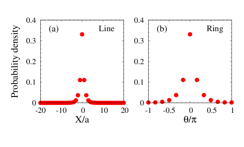
Figure 2: (Color online) The probability density of localized state for the one-dimensional scheme where the ring contains 11 lattice points. (a) The probability density on the wire. (b) The probability density on the ring. The intersection of the ring and the wire is at 0 both in (a) and (b)

For the one-dimensional model ($L_{W}{\to}0$), we take the ring size $Cl_{ring}=12a$, i.e., the ring contains 11 lattice points. The diagonalization of the one-dimensional structure Hamiltonian $H_{S}+H_{W}+H_{CS}$ shows that there exists only one localized state trapped at the intersection (shown in Fig. 2) with energy lying below the energy band. Moreover, the energy of this localized state $E$ is around $-0.310t$, which is close to the energy of the localized state in one-dimensional cross-shaped structure with the same on-site and hopping energy parameters.Openov The transmission therefore only shows the oscillatory behavior due to the structure resonance and antiresonance as shown in Fig. 3(a), where the transmission amplitude is plotted against the Fermi energy $E$ in the absence of magnetic flux. Moreover, the corresponding resonant energies in transmission, except the two outermost resonances which are close to the energy band edges, coincide with the eigenvalues of the isolated mesoscopic ring with the same size.Maiti The energies of the two outermost resonances are also very close to the eigenvalues of the isolated mesoscopic ring. In Fig. 3(b), we plot the transmission amplitudes of one resonance against the Fermi energy $E$ with different magnetic fluxes $\Phi$. One observes that the resonance peak doubles when ${\Phi}{\neq}0$ since the magnetic flux breaks the symmetry of the clockwise and counter-clockwise propagation on the ring, and the two resonance peaks shifted in the opposite directions with increasing the magnetic flux. Particularly, when ${\Phi}/{\Phi}_{0}=0.5$, the resonance and the antiresonance interchange the position in contrast to ${\Phi}/{\Phi}_{0}=0$ by comparing Figs. 3(a) and (c). When ${\Phi}/{\Phi}_{0}=1$, the transimission spectrum returns to the case with ${\Phi}/{\Phi}_{0}=0$ due to the periodicity of the magnetic flux. It is noted that we neglect the effect of the magnetic flux on the left and right leads in the computation. This is because that the AB phase coherence is due to the phase accumulated in a closed path rather than the phase accumulated on the leads. Our calculations also confirm that there is no difference for the results with/without the magnetic flux on the leads.

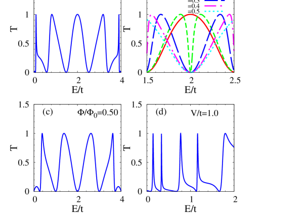
Figure 3: (Color online) Transmission amplitude $T$ vs Fermi energy of the leads for one-dimensional scheme, (a) with the magnetic flux ${\Phi}/{\Phi}_{0}=0$, (b) with different magnetic fluxes, (c) with the magnetic flux ${\Phi}/{\Phi}_{0}=0.5$, (d) with an on-site gate voltage $V=1.0t$ at the intersection and ${\Phi}/{\Phi}_{0}=0$.

Following the idea of introducing the localized state into the energy band, we lift the energy of the localized state by using an on-site gate voltage. We apply a positive voltageLiao $V=1.0t$ in the region where the probability density of the localized state is larger than $0.1$ (as show in Fig. 2, including the intersection point, two points on the line and two points on the ring). We find that the energy of the localized state is lifted to $E=0.54t$. The transmission amplitudes against the Fermi energy are plotted in Fig. 3(d), where one observes that the asymmetric Fano line shape appears at $E=0.60t$.

III.2 Localized states and transport properties in quasi-one-dimensional model

For the quasi-one-dimensional model in practice, the diagonalization of the structure Hamiltonian $H_{S}+H_{W}+H_{CS}$ shows that there exist localized states trapped at the intersection with energies lying below the each subband. The states which we are interested in are the ones whose energies lying inside the lowest subband. We find that when the inner radius of the ring $R$ is one order of magnitude smaller than the width $L_{W}$ of the wire, there exists only one localized state trapped at the intersection with energy lying inside the first subband. However, with increasing the inner radius of the ring $R$ under the same width $L_{W}$, two localized states appear in the first subband and tend to be degenerate. Geometrically, the increase of the inner radius separates the two positions where the ring intersects into the wire, the intersection then gradually evolves into two small equivalent intersections of the T-shaped structure. The two localized states embedded in the first subband concentrate at these two intersections. Since we are interested in the localized states due to the geometric confinement, we therefore concentrate on the case with small inner radius of the ring (one order of magnitude smaller than the width $L_{W}$ of the wire).

In Fig. 4, we plot the probability density of the localized state for the system with $R=2a$ and $L_{W}=18a$, and with the eigen-energy $E=0.0512t$ lying inside the first subband. One finds from the figure that for this localized state $\phi$ the electron indeed concentrates at the intersection, and decays exponentially away from the intersection. Moreover, the wave-function amplitude in the wire is small but finite, which implies that this localized state embedded in the first subband has a coupling ${\langle}{\phi}|H|{\Phi}{\rangle}$ with the continuum ones $\Phi$ and therefore manifests a quasi-localized behavior. For the system with different inner radii $R$ under the same width $L_{W}$, the coupling ${\langle}{\phi}|H|{\Phi}{\rangle}$ mainly comes from the region where the localized state concentrates and the localized state trapped at a larger region has a stronger coupling (larger wave-function amplitude in the wire). Furthermore, we also find the adjustment of the magnetic flux has little influence on the position of the localized state trapped at the intersection in the energy spectrum.

Figure 4: (Color online) The probability density of the quasi-bound state for the system with $L_{W}=18a$, $R=2a$ and ${\Phi}/{\Phi}_{0}=0.5$ with eigen-energy $E=0.0512t$.

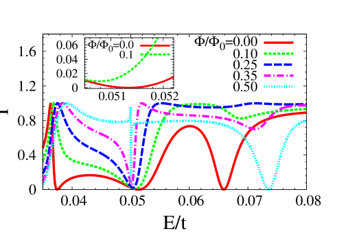
Figure 5: (Color online) Transmission amplitude $T$ vs Fermi energy of the leads with different magnetic fluxes when $L_{W}=18a$ and $R=2a$.

Figure 6: (Color online) Transmission amplitude $T$ vs Fermi energy of the leads with different disorder strengths $W$ when $L_{W}=18a$, $R=2a$ and ${\Phi}/{\Phi}_{0}=0$, (a) with both the Fano antiresonance and the structure antiresonance. (b) with an ordinary structure antiresonance.

In Fig. 5, we plot the transmission amplitudes against the Fermi energy for the system with $R=2a$ and $L_{W}=18a$, but with different magnetic fluxes. The energy window we choose in the figure lies inside the first subband. One finds that the asymmetric Fano line shape appears at the vicinity of $E=0.0512t$. The position of the Fano line shape coincides with the corresponding localized state obtained from the diagonalization. One observes that the magnetic flux has little effect on the position of the Fano line shape but has a marked influence on its shape. This interesting modulation is caused by the shift of the structure resonance which has been demonstrated in the case of one-dimensional model in the previous subsection. When the Fano dip is close to an antiresonance dip (${\Phi}/{\Phi}_{0}=0$), a wide energy gap $[0.051t,0.052t]$ appears in the transmission (see the red solid curve). Moreover, this gap can be turned off via tuning the magnetic flux. Specifically, when the Fano dip is close to a resonance peak (${\Phi}/{\Phi}_{0}=0.5$), a sharp dip with a sharp peak nearby appears in the transmission and a large transmission amplitude $T{\approx}0.8$ is obtained for the gap window $[0.051t,0.052t]$ (see the blue dotted curve). This feature demonstrates that the energy gap can be turned off or on by tuning the magnetic flux. Therefore, this model can work as a transistor with on and off features by tuning the magnetic flux.

We now show the feasibility of the above proposed model for a real application by analyzing the robustness of the energy gap against the Anderson disorder. In our simulation, the Anderson disorder is introduced by generating random on-site energies at the structure sites: ${\varepsilon_{0}}^{\prime}={\varepsilon_{0}}+{\xi}W$ in Eq. (3). Here $W$ is the Anderson disorder strength and ${\xi}$ is a random number with a uniform probability distribution in the range $(\mbox{-}1,1)$. The converged transmission amplitudes, which are averaged over 3000 random configurations for $R=2a$ and $L_{W}=18a$, are plotted in Fig. 6(a) against the Fermi energy in the vicinity of the energy gap with different Anderson disorder strengths $W$. One finds that the vanishingly small transmission amplitudes in the gap window $[0.051t,0.052t]$ become larger as the disorder strength $W$ increases. But even for the very large disorder strength $W=0.04t$, the corresponding transmission amplitudes for the gap window are still smaller than $0.04$, which is one order of magnitude smaller than the “on” transmission amplitudes $0.8$ as mentioned above. For comparison, we also show the robustness of an ordinary antiresonance (with the energy window $[0.0660,0.0666]$ and ${\Phi}/{\Phi}_{0}=0$) without a Fano antiresonance nearby in Fig. 6(b). The transmission amplitudes in this energy window rapidly increase with the strength of the disorder. Specifically, they already reach over $0.15$ at $W=0.03t$. Therefore, the transistors only based on the structure antiresonance are very weak against the disorder.

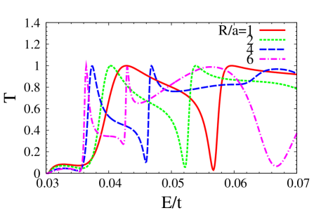
Figure 7: (Color online) Transmission amplitude $T$ vs Fermi energy of the leads with different inner radii $R$ of the ring when $L_{W}=18a$ and ${\Phi}/{\Phi}_{0}=0.35$.

In Fig. 7, we plot the transmission amplitudes against the Fermi energy for the system with $L_{W}=18a$ and ${\Phi}/{\Phi}_{0}=0.35$ but with different inner radii $R$, one observes that the asymmetric Fano antiresonance dip which appears in transmission when $R=a$ (see the red solid curve) gradually fades away with increasing the inner radius of the ring under the same width $L_{W}=18a$. Especially, when $R=6a$ under the same width $L_{W}=18a$, this dip in transmission is barely visible and two sharp resonance peaks appear (see the pink chain curve). As mentioned above, under the same width $L_{W}$, the increase of the inner radius separates the intersection into two small ones and there appear two localized states each trapped at a small intersection. Since the strength of the coupling ${\langle}{\phi}|H|{\Phi}{\rangle}$ between the localized state ${\phi}$ and the continuum ones ${\Phi}$ depends on the area of the localized region, these two localized states trapped at the small intersection therefore have weak couplings with the continuum ones, leading to two sharp resonance peaks in the transmission.

IV SUMMARY

In summary, we have extended a special kind of localized state trapped at the intersection due to the geometric confinement, first proposed in a three-terminal-opening T-shaped structure,Openov into a ring geometry with a tangent connection to the wire. This kind of the localized states has long been overlooked in the ring geometry attached to the wire. In this ring geometry, where we use a magnetic flux to thread the ring for modulation, we find that when the inner radius of the ring is one order of magnitude smaller than the width of the attached wire, there exists one localized state trapped at the intersection with energy lying inside the lowest subband. The Fano-type interference due to the coupling between this localized state and the continuum ones strongly modulates the transmission, leading to a Fano line shape. However, the increase of the inner radius of the ring weakens this coupling and the asymmetric Fano dip fades away. By tuning the magnetic flux for the structure with small inner radius of the ring, we find that a wide energy gap appears in the transmission when the Fano antiresonance and the structure antiresonance are close to each other. We propose that our structure can be used as a transistor since large transmission amplitudes can be obtained in the same energy gap region when the two types of the antiresonance are tuned away from each other by changing the magnetic flux. We also demonstrate the strong robustness of this energy gap against the Anderson disorder (in contrast to an ordinary structure antiresonance). Such features suggest that the proposed structure has great potential to work as transistors for a real application.

- (1) Y.-K. Lin, Y.-N. Chen, and D.-S. Chuu, Phys. Rev. B 64, 193316 (2001).
- (2) L. A. Openov, Euro. Phys. Lett. 55, 539 (2001).
- (3) F. Sols, M. Macucci, U. Ravaioli, and K. Hess, Appl. Phys. Lett. 54, 350 (1989).
- (4) Science and Engineering of One- and Zero-dimensional Semiconductors, edited by S. P. Beaumont and C. M. S. Torres (Springer, Berlin, 1990), p. 107.
- (5) X. Y. Feng, J. H. Jiang, and M. Q. Weng, Appl. Phys. Lett. 90, 142503 (2007).
- (6) K. Shen and M. W. Wu, Phys. Rev. B 77, 193305 (2008).
- (7) H. Tong and M. W. Wu, Phys. Rev. B 85, 205433 (2012).
- (8) J. G. Xu, L. Wang, and M. Q. Weng, J. Appl. Phys. 114, 153701 (2013).
- (9) U. Fano, Phys. Rev. 124, 1866 (1961).
- (10) A. E. Miroshnichenko, S. Flach, and Y. S. Kivshar, Rev. Mod. Phys. 82, 2257 (2010).
- (11) Y. Aharonov and D. Bohm, Phys. Rev. 115, 485 (1959).
- (12) Y. Gefen, Y. Imry, and M. Ya. Azbel, Phys. Rev. Lett. 52, 129 (1984).
- (13) Y. Aharonov and A. Casher, Phys. Rev. Lett. 53, 319 (1984).
- (14) M. V. Berry, Proc. R. Soc. London 392, 45 (1984).
- (15) R. A. Webb, S. Washburn, C. P. Umbach, and R. B. Laibowitz, Phys. Rev. Lett. 54, 2696 (1985).
- (16) L. P. Lévy, G. Dolan, J. Dunsmuir, and H. Bouchiat, Phys. Rev. Lett. 64, 2074 (1990).
- (17) V. Chandrasekhar, R. A. Webb, M. J. Brady, M. B. Ketchen, W. J. Gallagher, and A. Kleinsasser, Phys. Rev. Lett. 67, 3578 (1991).
- (18) D. Mailly, C. Chapelier, and A. Benoit, Phys. Rev. Lett. 70, 2020 (1993).
- (19) J. Nitta, F. E. Meijer, and H. Takayanagi, Appl. Phys. Lett. 75, 695 (1999).
- (20) A. G. Mal’shukov, V. V. Shlyapin, and K. A. Chao, Phys. Rev. B 60, R2161 (1999).
- (21) A. Fuhrer, S. Lüscher, T. Ihn, T. Heinzel, K. Ensslin, W. Wegscheider, and M. Bichler, Nature (London) 413, 822 (2001).
- (22) D. Frustaglia, M. Hentschel, and K. Richter, Phys. Rev. Lett. 87, 256602 (2001).
- (23) J. Nitta, T. Koga, and H. Takayanagi, Physica E 12, 753 (2002).
- (24) A. G. Mal’shukov, V. V. Shlyapin, and K. A. Chao, Phys. Rev. B 66, 081311(R) (2002).
- (25) M. Popp, D. Frustaglia, and K. Richter, Nanotechnology 14, 347 (2003).
- (26) R. Ionicioiu and I. D’Amico, Phys. Rev. B 67, 041307(R) (2003).
- (27) D. Frustaglia and K. Richter, Phys. Rev. B 69, 235310 (2004).
- (28) M. Hentschel, H. Schomerus, D. Frustaglia, and K. Richter, Phys. Rev. B 69, 155326 (2004).
- (29) D. Frustaglia, M. Hentschel, and K. Richter, Phys. Rev. B 69, 155327 (2004).
- (30) R. Capozza, D. Giuliano, P. Lucignano, and A. Tagliacozzo, Phys. Rev. Lett. 95, 226803 (2005).
- (31) M. König, A. Tschetschetkin, E. M. Hankiewicz, J. Sinova, V. Hock, V. Daumer, M. Schäfer, C. R. Becker, H. Buhmann, and L. W. Molenkamp, Phys. Rev. Lett. 96, 076804 (2006).
- (32) T. Bergsten, T. Kobayashi, Y. Sekine, and J. Nitta, Phys. Rev. Lett. 97, 196803 (2006).
- (33) F. Qu, F. Yang, J. Chen, J. Shen, Y. Ding, J. Lu, Y. Song, H. Yang, G. Liu, J. Fan, Y. Li, Z. Ji, C. Yang, and L. Lu, Phys. Rev. Lett. 107, 016802 (2011).
- (34) F. Nagasawa, J. Takagi, Y. Kunihashi, M. Kohda, and J. Nitta, Phys. Rev. Lett. 108, 086801 (2012).
- (35) F. Nagasawa, D. Frustaglia, H. Saarikoski, K. Richter, and J. Nitta, Nat. Commun. 4, 2526 (2013).
- (36) F. K. Joibari, Ya. M. Blanter, and G. E. W. Bauer, Phys. Rev. B 88, 115410 (2013).
- (37) A. Chaves, G. A. Farias, F. M. Peeters, and B. Szafran, Phys. Rev. B 80, 125331 (2009).
- (38) M. R. Poniedzialek and B. Szafran, J. Phys.: Condens. Matter 22, 465801 (2010).
- (39) M. P. Nowak, B. Szafran, and F. M. Peeters, Phys. Rev. B 84, 235319 (2011).
- (40) M. Büttiker, Phys. Rev. Lett. 57, 1761 (1986).
- (41) S. Datta, Electronic Transport in Mesoscopic Systems (Cambridge University Press, New York, 1995).
- (42) P. G. Silvestrov and K. B. Efetov, Phys. Rev. Lett. 98, 016802 (2007).
- (43) P. Recher, J. Nilsson, G. Burkard, and B. Trauzettel, Phys. Rev. B 79, 085407 (2009).
- (44) S. K. Maiti, Physica E 36, 199204 (2007).
- (45) L. Liao, J. W. Bai, R. Cheng, Y. C. Lin, S. Jiang, Y. Huang, and X. F. Duan, Nano Lett. 10, 1917 (2010).