Understanding Dynamic Graphs:
The Case for Centrality Distance

Modeling and Measuring Graph Similarity:
The Case for Centrality Distance

Abstract

The study of the topological structure of complex networks has fascinated researchers for several decades, and today we have a fairly good understanding of the types and reoccurring characteristics of many different complex networks. However, surprisingly little is known today about models to compare complex graphs, and quantitatively measure their similarity.

This paper proposes a natural similarity measure for complex networks: centrality distance, the difference between two graphs with respect to a given node centrality. Centrality distances allow to take into account the specific roles of the different nodes in the network, and have many interesting applications. As a case study, we consider the closeness centrality in more detail, and show that closeness centrality distance can be used to effectively distinguish between randomly generated and actual evolutionary paths of two dynamic social networks.

1 Introduction

How similar are two graphs $G_{1}$ and $G_{2}$? Surprisingly, today, we do not have good measures to answer this question. In graph theory, the canonical measure to compare two graphs is the Graph Edit Distance (GED) [8]: informally, the GED $d_{\textsc{GED}}(G_{1},G_{2})$ between two graphs $G_{1}$ and $G_{2}$ is defined as the minimal number of graph edit operations that are needed to transform $G_{1}$ into $G_{2}$. The specific set of allowed graph edit operations depends on the context, but typically includes some sort of node and link insertions and deletions.

While graph edit distance metrics play an important role in computer graphics and are widely applied to pattern analysis and recognition, we argue that the graph edit distance is not well-suited for measuring similarities between natural and complex networks. The set of graphs at a certain graph edit distance $d$ from a given graph $G$, are very diverse and seemingly unrelated: the characteristic structure of $G$ is lost.

A good similarity measure can have many important applications. For instance, a similarity measure can be a fundamental tool for the study of dynamic networks, answering questions like: Do these two complex networks have a common ancestor? Or: What is a likely successor network for a given network? While the topological properties of complex networks have fascinated researchers for many decades, (e.g., their connectivity [1, 14], their constituting motifs [13], their clustering [18] or community patterns [3]), today, we do not have a good understanding of their dynamics over time.

Our Contributions. This paper initiates the study of graph similarity measures for complex networks which go beyond simple graph edit distances. In particular, we introduce the notion of centrality distance $d_{C}(G_{1},G_{2})$, a graph similarity measure based on a node centrality $C$.

We argue that centrality-based distances are attractive similarity measures as they are naturally node-oriented. This stands in contrast to, e.g., classic graph isomorphism based measures which apply only to anonymous graphs; in the context of dynamic complex networks, nodes typically do represent real objects and are not anonymous!

We observe that the classic graph edit distance can be seen as a special case of centrality distance: the graph edit distance is equivalent to the centrality distance where $C$ is simply the degree centrality, henceforth referred to as the degree distance $d_{\textsc{DC}}$. We then discuss alternative centrality distances and, as a case study, explore the closeness distance $d_{\textsc{CC}}$ (based on closeness centrality) in more detail.

In particular, we show that closeness distance has interesting applications in the domain of dynamic network prediction. As a proof-of-concept, we consider two dynamic social networks: (1) An evolving network representing the human mobility during a cocktail party, and (2) a Facebook-like Online Social Network (OSN) evolving over time. We show that actual evolutionary paths are far from being random from the perspective of closeness centrality distance, in the sense that the distance variation along evolutionary paths is low. This can be exploited to distinguish between fake and actual evolutionary paths with high probability.

Examples. To motivate the need for graph similarity measures, let us consider two simple examples.

Example 1.1 (Local/Global Scenario)

We consider three graphs $G_{1}$, $G_{2}$, $G_{3}$ over five nodes $\{v_{1},v_{2},\ldots,v_{5}\}$: $G_{1}$ is a line, where $v_{i}$ and $v_{i+1}$ are connected in a modulo manner; $G_{2}$ is a cycle, i.e., $G_{1}$ with an additional link $\{v_{1},v_{5}\}$; and $G_{3}$ is $G_{1}$ with an additional link $\{2,4\}$.

In this example, we first observe that $G_{2}$ and $G_{3}$ have the same graph edit distance to $G_{1}$: $d_{\textsc{GED}}(G_{1},G_{2})=d_{\textsc{GED}}(G_{1},G_{3})=1$, as they contain one additional edge. However, in a social network context, one would intuitively expect $G_{3}$ to be closer to $G_{1}$ than $G_{2}$. For example, in a friendship network a short-range “triadic closure” [10] link may be more likely to emerge than a long-range link: friends of friends may be more likely to become friends themselves in the future. Moreover, more local changes are also expected in mobile environments (e.g., under bounded human mobility and speed). As we will see, the centrality distance concept introduced in this paper can capture such differences.

Example 1.2 (Evolution Scenario)

As a second artificial and very simple example, in this paper we will consider two graphs $G_{1}$ and $G_{2}$, where $G_{1}$ is a line topology and $G_{2}$ is a “shell network”, shown in Figure 1. We ask the question: what is the most likely evolutionary path that would lead from the $G_{1}$ topology to $G_{2}$?

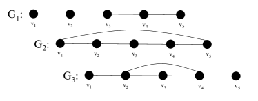
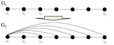
Figure 1: Left: Local/Global Scenario: $G_{1}$ is a line graph, $G_{2}$ and $G_{3}$ are obtained from $G_{1}$ by adding a link. Right: Evolution Scenario: $G_{1}$ describes a line graph, $G_{2}$ describes a shell graph.

Note that the graph edit distance does not provide us with any information about the likely evolutionary paths from $G_{1}$ to $G_{2}$, i.e., on the order of the edge insertions: there are many possible orders in which the missing links can be added to $G_{1}$, and these orders do not differ in any way. In reality, however, we often have some expectations on how a graph may have evolved between the two given snapshots $G_{1}$ and $G_{2}$. For example, applying the triadic closure principle to our example, we would expect that the missing links are introduced one-by-one, from left to right. A similar evolution may also be predicted by a temporal preferential attachment model [14]: the degree of the most highly connected node is likely to grow further in the future.

The situation may look different in a technological, man-planned network. For example, adding links from left to right only slowly improves the “routing efficiency” of the network: after the addition of $t$ edges from left to right, the longest shortest path is $n-t$ hops, for $t<n-1$. A “better” evolution of the network can be obtained by adding links to the middle of the network, reducing the much faster in the beginning: after $t$ edge insertions, the distance is roughly reduced by a factor $t$.

2 Model and Background

This paper focuses on named (a.k.a. labeled) graphs $G=(V,E)$: graphs where vertices $v\in V$ have unique identifiers and are connected via undirected edges $e\in E$. We focus on node centralities, centralities assigning “importance values” to nodes $v\in V$.

Definition 2.1 (Centrality)

A centrality $C$ is a function $C\colon(G,v)\to\mathbb{R}^{+}$ that takes a graph $G=(V,E)$ and a vertex $v\in V(G)$ and returns a positive value $C(G,v)$. The centrality function is defined over all vertices $V(G)$ of a given graph $G$. Although we here consider named graphs, we require centrality values of vertices to be independent of the vertex’s identifier, i.e., centralities are unchanged by a permutation of identifiers: given any permutation $\pi$ of $V(G)$, $\forall v\in V(G),C(\pi(G),\pi(v))=C(G,v)$, where $\pi(G)=(V(G),\{(\pi(v),\pi(v^{\prime})):(v,v^{\prime})\in E(G)\}$.

Centralities are a common way to characterize complex networks and their vertices. Frequently studied centralities include the degree centrality (DC), the betweenness centrality (BC) and the closeness centrality (CC), among many more. A node is DC-central if it has many edges: the degree centrality is simply the node degree; a node is BC-central if it is on many shortest paths: the betweenness centrality is the number of shortest paths going through the node; and a node is CC-central if it is close to many other nodes: the closeness centrality measures the inverse of the distances to all other nodes. Formally:

1. Degree Centrality: For any node $v\in V(G)$ of a network $G$, let $\Gamma(v)$ be the set of neighbors of node $v$: $\Gamma(v)=\{w\in V\textrm{s.t.~{}}\{v,w\}\in E\}$. The degree centrality DC of a node $v\in V$ is defined as: $\textsc{DC}(G,v)=|\Gamma(v)|$.

2. Betweenness Centrality: For any pair $(v,w)\in E(G)$, let $\sigma(v,w)$ be the total number of different shortest paths between $v$ and $w$, and let $\sigma_{x}(v,w)$ be the number of shortest paths between $v$ and $w$ that pass through $x\in V$. The betweenness centrality BC of a node $v\in V$ is defined as: $\textsc{BC}(G,v)=\sum_{x,w\in V}\sigma_{v}(x,w)/\sigma(x,w)$. As a slight variation from the classic definition, we assume that a node is on its own shortest path: $\forall v,w\in V^{2},\sigma_{v}(v,w)/\sigma(v,w)=1$. We adopt the convention: $\forall v\in V,\sigma_{v}(v,v)/\sigma(v,v)=0$. The reason of this variation will become clear in the next section.

3. Closeness Centrality: The closeness centrality CC of a node $v\in V$ is defined as: $\textsc{CC}(G,v)=\sum_{w\in V\setminus v}2^{-d(v,w)}$.

By convention, we define the centrality of a node with no edges to be 0. Moreover, throughout this paper, we will define the graph edit distance between two graphs $G_{1}$ and $G_{2}$ as the minimum number of operations to transform $G_{1}$ into $G_{2}$ (or vice versa), where an operation is one of the following: link insertion, link removal, node insertion, node removal.

3 Graph Distances

We now introduce our centrality-based graph similarity measure. We will refer to the set of all possible topologies by $\mathcal{G}$, and we will sometimes think of $\mathcal{G}$ being a graph itself: the “graph-of-graphs” which connects graphs with graph edit distance 1. Figure 2 illustrates the concept.

Definition 3.1 (Centrality Distance)

Given a centrality $C$, we define the centrality distance $d_{C}(G_{1},G_{2})$ between two neighboring graphs as the component-wise difference:

$$\forall(G_{1},G_{2})\in E(\mathcal{G}),d_{C}(G_{1},G_{2})=\sum_{v\in V}|C(G_{1},v)-C(G_{2},v)|.$$

This definition extends naturally for non-neighboring graph couples: the distance $d_{C}(G_{1},G_{2})$ between $G_{1}$ and $G_{2}$ is simply the graph-induced distance.

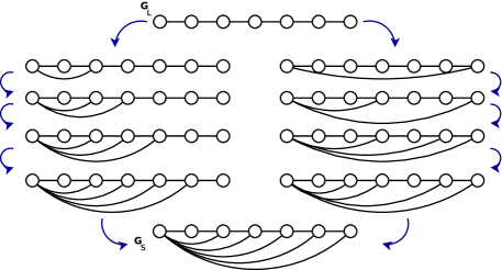
Figure 2: Left: The graph-of-graph $\mathcal{G}$ connects named networks (represented as stars). Two networks are neighboring iff they differ by a graph edit distance of one. The centrality distance defines a distance for each pair of neighboring graphs. Right: Two possible evolutionary paths from a line graph $G_{1}$ to a shell graph $G_{2}$.

As we will see, the distance axioms are indeed fulfilled for the major centralities. The resulting structure supports the formal study with existing algorithmic tools. Let us first define the notion of sensitivity.

Definition 3.2 (Sensitive Centrality)

A centrality $C$ is sensitive if any single edge modification of any graph $G$ changes the centrality value of at least one node of $G$. Formally, a centrality $C$ is sensitive iff

$$\forall G\in\mathcal{G},\forall e\in E(G),\exists v\in V(G)\textrm{ s.t. }C(G,v)\neq C(G\setminus\{e\},v),$$

where $G\setminus\{e\}$ is the result of removing edge $e$ from $G$.

Lemma 3.3

DC, BC and CC are sensitive centralities.

It is easy to see that also other centralities, such as cluster centralities and Page Rank centralities are sensitive. The distance axioms now follow directly from the graph-induced distance.

Theorem 3.4

For any centrality $C$, $d_{C}$ is a distance on $\mathcal{G}$ iff $C$ is sensitive.

The centrality distance metric of Definition 3.1 however comes with the drawback that it is expensive to compute. Thus, we propose the following approximate version:

Definition 3.5 (Approximate Centrality Distance)

Given a centrality $C$, we define the approximate centrality distance $\widetilde{d_{C}}(G_{1},G_{2})$ between any two graphs as the component-wise difference:

$$\forall(G_{1},G_{2}),\widetilde{d_{C}}(G_{1},G_{2})=\sum_{v\in V}|C(G_{1},v)-C_{2}(G_{2},v)|.$$

Note that $\widetilde{d_{C}}\leq d_{C}$ always holds. As we will see, while the approximate distance can be far from the exact one in the worst case, it features some interesting properties.

4 Example: Closeness Distance

To illustrate the concepts, we will follow the example of a topological evolution changing a line graph into a shell graph (depicted in Figure 2 (right)). This figure shows two different paths: $A$ incrementally connects node $v_{1}$ to node $v_{i}$ for $i=3,\ldots,n$, whereas path $B$ dichotomically connects $v_{i}$ to nodes $v_{n},v_{n/2},v_{3n/4},v_{n/4},v_{7n/8},v_{5n/8},\ldots$.

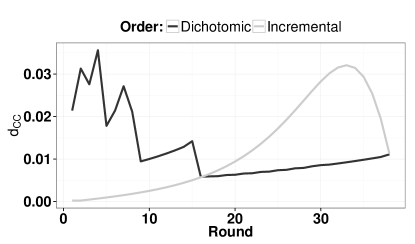
Figure 3: Evolution of closeness centrality distance $d_{CC}$ from $G_{L}$ to $G_{S}$ for $n=40$. Dichotomic and incremental paths are depicted in Figure 2 (right). Both order define a different path in $\mathcal{G}$ from $G_{L}$ to $G_{S}$. At each step, the closeness centrality-induced distance between $G_{i}$ and $G_{i-1}$ is computed.

4.1 Degree Distance

As a baseline and for comparison with alternative centralities, we will consider the degree distance $d_{\textsc{DC}}(G_{1},G_{2})$: the distance between two graphs simply counts the number of different edges. We first make the simple observation that the number of graph edits is equivalent to the differences in the centrality vectors.

Observation 1

The graph edit distance is equivalent to the degree distance, i.e., $d_{\textsc{GED}}\equiv d_{\textsc{DC}}$.

This connection is established by the topological shortest path in the graph-of-graphs $\mathcal{G}$. Let us consider our example from Figure 2 (right): Since all paths from $G_{1}$ to $G_{2}$ which do not introduce unnecessary edges have the same cost, the order in which edges are inserted is irrelevant. From a $d_{\textsc{GED}}$ perspective the incremental (left) and the dichotomic (right) paths of Figure 2 (right) are equivalent.

We make the following observation:

Observation 2

The degree distance resp. graph edit distance does not provide much insights into graph evolution paths: essentially all paths have the same costs.

4.2 Closeness Distance

Intuitively, a high closeness distance indicates a large difference in the distances of the graph. The closeness distance $d_{\textsc{CC}}$ has some interesting properties. For example, the shortest path in the graph-of-graph is connected the the topological shortest path. In particular, if two graphs are related by inclusion, the shortest closeness path is also a topological shortest path, as shown in the following.

Theorem 4.1

Let $G_{1}$ and $G_{2}$ two graphs in $\mathcal{G}$ such that $E(G_{1})\subset E(G_{2})$. Then all the topological shortest paths (i.e. paths that only add edges from $G_{1}$ to $G_{2}$) are equivalent for closeness.

The inclusion property is a relevant property in many temporal networks, e.g., where links do not age (e.g. if an edge denotes that $u$ has ever met/traveled/read $v$).

To give some intuition of the closeness distance, Figure 4 plots the evolution of the distance terms over time. As we can see, in the dichotomic order, first longer links are added, while the first incremental steps are more or less stable.

The dichotomic path has the larger impact on the dynamic graph’s shortest path distances. This indicates that the closeness distance could even be used for “greedy routing”, in the sense that efficient topological evolutions can be computed by minimizing the distance to a target topology.

5 Experimental Case Studies

This section studies the power and limitation of closeness distance empirically, in two case studies: the first scenario is based on a data set we collected during a cocktail party and models a human mobility pattern; the second scenario is based on an evolving online social network (OSN) data set which is publicly available.

Datasets. The first case study is based on the SOUK dataset [9]. This dataset captures the social interactions of 45 individuals during a cocktail, see [9] for more details. The dataset consists in $300$ discrete timesteps, describing the dynamic interaction graph between the participants, one timesteps every $3$ seconds.

The second case study is based on a publicly available dataset FBL [15], capturing all the messages exchanges realized on an online Facebook-like social network between roughly 20k users over 7 months. We discretized the data into a dynamic graph of 187 timesteps representing the daily message exchanges among users. For each of these two graphs series, we compare each graph $G_{t}$ with the subsequent one: $G_{a}=G_{t}$,$G_{b}=G_{t+1}$. First, we generate a set $S$ of $200$ samples such that $\forall G_{2}\in S,d_{\textsc{GED}}(G_{a},G_{2})=d_{\textsc{GED}}(G_{a},G_{b})$. Then we compare the centrality induced distance $d_{C}$ from $G_{a}$ to the samples of $S$ against $d_{C}(G_{a},G_{b})$.

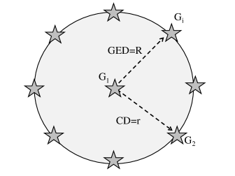
Figure 4: Illustration of our methodology: Given an initial graph $G_{1}$, graphs $G_{i}$ at a given graph edit distance $d_{\textsc{GED}}=R$ are generated uniformly at random. The actual later graph observed in the experiment is denoted by $G_{2}$. We test the hypothesis that $G_{2}$ is closer to $G_{1}$ than other graphs $G_{i}$ with respect to a certain centrality distance $d_{C}$.

Methodology. We study the question whether centrality distances could be used to predict the evolution of a temporally evolving network. To this end, we introduce a simple methodology: We take a graph $G_{1}$ and a graph $G_{2}$ following $G_{1}$ later in time in the given experiment. For these two graphs, the graph edit distance (or “radius”) $R:=d_{\textsc{GED}}(G_{1},G_{2})$ is determined, and we generate alternative graphs $G_{i}$ at the same graph edit distance $R$ uniformly at random. We investigate the question whether closeness centrality distance can help to effectively distinguish $G_{2}$ from other graphs $G_{i}$, in the sense that $d_{CC}(G_{1},G_{2})\ll d_{CC}(G_{1},G_{i})$ for $i\neq 2$. Figure 4 illustrates our methodology.

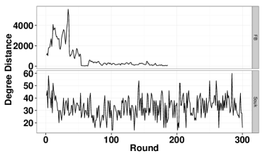
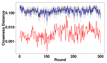
Figure 5: Left: Measured closeness distance $d_{C}$ from $G_{t}$ to $G_{t+1}$ (red), and to $S_{t+1}$ sampled graphs (blue: median, bars: 5 and 95 percentiles) over time. Right: Temporal representation of the measured closeness distance $d_{\textsc{CC}}$ from $G_{t}$ to $G_{t+1}$ (red) on the SOUK dataset, and to $S_{t+1}$ sampled graphs (blue: median, bars: 5 and 95 percentiles) over time.

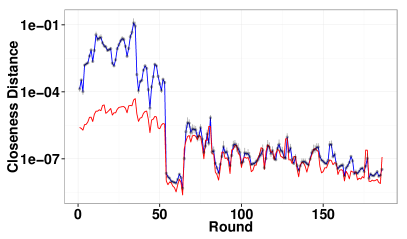
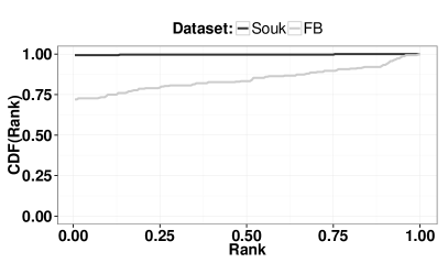
Figure 6: Left: Temporal representation of the measured closeness distance $d_{\textsc{CC}}$ from $G_{t}$ to $G_{t+1}$ (red) on the FB dataset, and to $S_{t+1}$ sampled graphs (blue: median, bars: 5 and 95 percentiles) over time. Right: CDF of the rank of the measured topology closeness distance among the closeness distances to the sampled equivalent topologies for both datasets.

Results. Figure 5 (left) provides a temporal perspective on the evolution of $d_{\textsc{GED}}$ for both the 300 timesteps of the SOUK dynamic graph and the 187 timesteps of the FB dataset. Both datasets exhibit very different dynamics: FB has a high dynamics for the first 50 timestemps, and is then relatively stable, whereas SOUK exhibits a more regular dynamics.

Figure 5 (right) presents the results of our experiment on the SOUK dataset. It represents the closeness distance $d_{\textsc{CC}}$ from each graph $G_{t}$ to $G_{t+1}$ in red. The distribution of $d_{\textsc{CC}}$ values from $G_{t}$ to the $200$ randomly sampled graphs of $S_{t+1}$ is represented as follows: the blue line is the median, while the gray lines represent the $5$ and $95$ percentiles of the distribution. One can observe that although $\forall G_{2}\in S_{t+1},d_{\textsc{GED}}(G_{t},G_{2})=d_{\textsc{GED}}(G_{t},G_{t+1})$, most of the time $d_{\textsc{CC}}(G_{t},G_{t+1})\leq d_{\textsc{CC}}(G_{t},G_{2}),\forall G_{2}\in S_{t+1}$. In other words, most of the times, the measured graph $G_{t+1}$ is closer to $G_{t}$ in closeness distance than the $5\%$ closest randomly sampled graphs. Figure 6 (Left) presents the same results on the FB dataset. Here, although most of the time the measured topology is closer in closeness distance, this is mostly true for the first, most dynamic, time steps.

Figure 6 (right) provides a more aggregate view of this observation: it shows the rank of $d_{C}(G_{t},G_{t+1})$ in the $\{d_{C}(G_{t},G_{2}),G_{2}\in S_{t+1}\}$ distribution for the closeness (CC) centrality distance for both dynamic graphs. Values are sorted increasingly, so rank $0$ represents the smallest. This graph shows that out of the $300$ timesteps of SOUK, the observed graph is closer than any of the 200 random samples in $298$ timesteps for the closeness distance. The same statement holds for $73\%$ of the $187$ snapshots of the FB dataset.

The observation one can draw from this plot is that when we measure the raw evolution of topologies (in terms of degree distance) we only grasp a very incomplete, and rather pessimistic view of the dynamics on both datasets. Compared to a random evolution that would create the same degree distance difference, actual topology evolution leaves most of nodes importance as connectors (closeness distance) unchanged.

6 Related Work

To the best of our knowledge, our paper is the first to combine the important concepts of graph distances and centralities. In the following, we will review the related works in the two fields in turn, and subsequently discuss additional literature on dynamic graphs.

Graph distances. Graph edit distances have been used extensively in the context of inexact graph matchings in the field of pattern analysis. Central to this approach is the measurement of the similarity of pairwise graphs. Graph edit distances are attractive for their error-tolerance to noise. We refer the reader to the good survey by Gao et al. [8] for more details.

However, we in this paper argue that the graph edit distance fails to capture important semantic differences, and are not well suited to measure similarities between complex networks. Accordingly, we introduce a distance which is based on a parameterizable centrality.

In classic graph theory, notions of similarity often do not take into account the individual nodes. A special case are graph isomorphism problems: The graph isomorphism problem is the computational problem of determining whether two finite graphs are isomorphic. While the problem is of practical importance, and has applications in mathematical chemistry, many complex networks and especially social networks are inherently non-anonymous. For example, for the prediction of the topological evolution of a network such as Facebook, or for predicting new topologies based on human mobility, individual nodes should be taken into account. Moreover, fortunately, testing similarity between named graphs is often computationally much more tractable.

Graph characterizations and centralities. Graph structures are often characterized by the frequency of small patterns called motifs [4, 13, 19, 17], also known as graphlets [16], or structural signatures [6]. Another important graph characterization, which is also studied in this paper, are centralities. [5] Dozens of different centrality indices have been defined over the last years, and their study is still ongoing, and a unified theory missing. We believe that our centrality distance framework can provide new inputs for this discussion.

Dynamic graphs. Researchers have been fascinated by the topological structure and the mechanisms leading to them for many years. While early works focused on simple and static networks [7], later models, e.g., based on preferential attachment [2], also shed light on how new nodes join the network, resulting in characteristic graphs. Nevertheless, today, only very little is known about the dynamics of social networks. This is also partly due to the lack of good data, which renders it difficult to come up with good methodologies for evaluating, e.g., link prediction algorithms [12, 20].

An interesting related work to ours is by Kunegis [11], who also studied the evolution of networks, but from a spectral graph theory perspective. In his thesis, he argues that the graph spectrum describes a network on the global level, whereas eigenvectors describe a network at the local level, and uses these results to devise link prediction algorithms.

7 Conclusion

We believe that our work opens a rich field for future research. In this paper, we mainly focused on closeness distance, and showed that it has interesting properties when applied to the use case of dynamic social networks. However, our early results indicate that other centralities have very interesting properties as well. For instance, it can be seen that using betweenness distance to move from a graph $G_{1}$ to a smaller graph $G_{2}$ results in the same graph sequence as Newman’s graph clustering algorithms, indicating that betweeness distance can be used to study graph clusterings over time. The properties, opportunities and limitations of alternative centralities will be the main focus of our future work.

Acknowledgments. Stefan Schmid is supported by the DAAD-PHC PROCOPE program, the EIT ICT project Mobile SDN, and is part of the INP visiting professor program. Gilles Tredan is supported by the DAAD-PHC PROCOPE program.

Appendix A Proof of Lemma 3.3

Let $G\in\mathcal{G}$, and $e=(u,v)\in E(G)$.

Degree centrality: $\textsc{DC}(G,u)=\textsc{DC}(G\setminus\{e\},u)+1$: DC is sensitive.

Betweenness centrality: Recall our slightly changed definition of betweenness. Now, $\textsc{BC}(G,u)=\sum_{x,w\in V}\sigma_{u}(x,w)/\sigma(x,w)$. In $G\setminus\{e\}$, all shortest paths are at least as long as in $G$, and the shortest path between $u$ and $v$ has increased at least one unit: BC is sensitive.

Closeness centrality: $\textsc{CC}(G,u)=\sum_{w\in V\setminus\{u\}}2^{-d(u,w)}$. In $G\setminus\{e\}$, all distances are greater or equal than in $G$, and strictly greater for the couple $(u,v)$: CC is sensitive.

Appendix B Proof of Theorem 3.4

We show that $d_{C}$ is a metric on $\mathcal{G}$:

Separation

$\forall G_{1},G_{2}\in\mathcal{G},d_{C}(G_{1},G_{2})\geq 0$ since all summands are non-negative.

Coincidence

If $G_{1}=G_{2}$, we have $\sum_{v\in V}|C_{1}(v)-C_{1}(v)|=0$. If $G_{1}\neq G_{2}$ and $C$ is sensitive, since $\forall G\in N(G_{1}),d_{C}(G_{1},G)>0$, necessarily $d_{C}(G_{1},G_{2})>0$. For the sake of contradiction, assume $C$ is not sensitive: $\exists G\in\mathcal{G},e\in E(G)$ s.t. $\forall v\in G,C(G,v)=C(G\setminus\{e\},v)$, and therefore $d_{C}(G,G\setminus\{e\})=0$ with $G\neq G\setminus\{e\}$: $d_{C}$ is not a metric.

Symmetry

Straightforward since $|C(G_{2},v)-C(G_{1},v)|=|C(G_{1},v)-C(G_{2},v)|$.

Triangle inequality

Observe that the neighbor-based $d_{C}$ definition associates each edge of $\mathcal{G}$ with a strictly positive weight. The multi-hop distance $d_{C}$ is the weighted shortest path in $\mathcal{G}$ given those weights. Since the weighted shortest path obeys the triangle inequality for strictly positive weights, $d_{C}$ does as well.

Appendix C Proof of Theorem 4.1

Let $P$ be a topological shortest paths connecting $G_{1}$ and $G_{2}$: $|P|=d_{\textsc{GED}}(G_{1},G_{2})$. Since $E(G_{1})\subset E(G_{2})$, $P$ contains only edge additions to $G_{1}$, where $|P|$ denotes the path length. Also $\forall u,v\in V^{2},\forall i,d_{P[i]}(u,v)\geq d_{P[i+1]}(u,v)$, where $P[i]$ denotes the $i$-th node on the path. Therefore $|\textsc{CC}(P[i],(v))-\textsc{CC}(P[i+1],(v))|=\textsc{CC}({P[i]},v)-\textsc{CC}(P[i+1],v)$.

Therefore:

$$d_{\textsc{CC}}(G_{1},G_{2}) \leq \sum_{i=1}^{|P|-1}d_{\textsc{CC}}(P[i],P[i+1])$$

$$= \sum_{i=1}^{|P|-1}\sum_{v\in V}\textsc{CC}(P[i],v)-\textsc{CC}(P[i+1],v)$$

$$= \sum_{v\in V}\textsc{CC}(G_{1},v)-\textsc{CC}(G_{2},v)$$

$$= {\widetilde{d}}_{\textsc{CC}}(G_{1},G_{2})\leq d_{\textsc{CC}}(G_{1},G_{2})$$

The sum of the closeness distances on this path $P$ is the exact closeness distance, for any such path $P$: all shortest paths are equivalent for $d_{\textsc{CC}}$ in this case.

References

- [1] Barabási, A.-L., and Albert, R. Emergence of Scaling in Random Networks. Science 286 (1999).
- [2] Barabasi, A.-L., and Albert, R. Emergence of scaling in random networks. Science 286 (1999).
- [3] Berry, J. W., Hendrickson, B., LaViolette, R. A., and Phillips, C. A. Tolerating the community detection resolution limit with edge weighting. In arXiv (2009).
- [4] Boccaletti, S., Latora, V., Moreno, Y., Chavez, M., and Hwang, D.-U. Complex networks: Structure and dynamics. Physics Reports 424, 4 5 (2006), 175 – 308.
- [5] Brandes, U., and Erlebach, T. Network Analysis: Methodological Foundations. LNCS 3418, Springer-Verlag New York, Inc., 2005.
- [6] Contractor, N. S., Wasserman, S., and Faust, K. Testing multitheoretical organizational networks: An analytic framework and empirical example. Academy of Management Review (2006).
- [7] Erdos, P., and R nyi, A. On the evolution of random graphs. In Math. Inst. Hungarian Academy of Sciences (1960), pp. 17–61.
- [8] Gao, X., Xiao, B., Tao, D., and Li, X. A survey of graph edit distance. Pattern Anal. Appl. 13, 1 (2010), 113–129.
- [9] Killijian, M.-O., Roy, M., Trédan, G., and Zanon, C. SOUK: Social Observation of hUman Kinetics. In Proc. ACM International Joint Conference on Pervasive and Ubiquitous Computing (UbiComp) (2013).
- [10] Kossinets, G., and Watts, D. J. Empirical analysis of an evolving social network. Science 311, 5757 (2006), 88–90.
- [11] Kunegis, J. On the spectral evolution of large networks. PhD thesis (2011).
- [12] Liben-Nowell, D., and Kleinberg, J. The link prediction problem for social networks. In Proc. 12th International Conference on Information and Knowledge Management (CIKM) (2003).
- [13] Milo, R., Shen-Orr, S., Itzkovitz, S., Kashtan, N., Chklovskii, D., and Alon, U. Network motifs: Simple building blocks of complex networks. In SCIENCE (2001).
- [14] Newman, M. Clustering and preferential attachment in growing networks. Phys. Rev. E (2001).
- [15] Opsahl, T., and Panzarasa, P. Clustering in weighted networks. Social networks 31, 2 (2009), 155–163.
- [16] Przulj, N. Biological network comparison using graphlet degree distribution. Bioinformatics (2007).
- [17] Schreiber, F., and Schwöbbermeyer, H. Frequency concepts and pattern detection for the analysis of motifs in networks. Transactions on Computational Systems Biology 3 (2005), 89–104.
- [18] Watts, D., and Strogatz, S. The small world problem. Collective Dynamics of Small-World Networks 393 (1998), 440–442.
- [19] Wernicke, S. Efficient detection of network motifs. IEEE/ACM Trans. Comput. Biol. Bioinformatics 3, 4 (Oct. 2006), 347–359.
- [20] Yang, S. H., Long, B., Smola, A., Sadagopan, N., Zheng, Z., and Zha, H. Like like alike: joint friendship and interest propagation in social networks. In Proc. 20th International Conference on World Wide Web (WWW) (2011), pp. 537–546.