Arcs, balls and spheres that cannot be attractors in $\mathbb{R}^{3}$

Abstract.

For any compact set $K\subseteq\mathbb{R}^{3}$ we define a number $r(K)$ that is either a nonnegative integer or $\infty$. Intuitively, $r(K)$ provides some information on how wildly $K$ sits in $\mathbb{R}^{3}$. We show that attractors for discrete or continuous dynamical systems have finite $r$ and then prove that certain arcs, balls and spheres cannot be attractors by showing that their $r$ is infinite.

1. Introduction

Many dynamical systems have an attractor, which is a compact invariant set $K$ such that every initial condition sufficiently close to $K$ approaches it as the system evolves (see Definition 1). Eventually the dynamics of the system will be indistinguishable from the dynamics on the attractor, and in this sense we may say that the attractor captures the long term behaviour of the system (at least for a certain range of initial conditions).

The structure of attractors as subsets of the phase space $M$ is frequently very intrincate, and this leads naturally to the following characterization problem:

“characterize topologically what compact sets $K\subseteq M$ can be an attractor for a dynamical system on $M$”.

Notice that no conditions are placed on the dynamics on the attractor: this is a very interesting variant of the problem (for instance, it arises in some questions related to partial differential equations; see Section 10.1), but almost intractable by our present knowledge. Also, the characterization will generally depend on $M$ and whether one is interested in discrete or continuous dynamical systems. The latter are well understood [11, 26] so we shall restrict ourselves to discrete dynamical systems.

Heuristically, solving the characterization problem requires that we identify the obstructions that prevent a set from being an attractor. For example, attractors have finitely generated Čech cohomology with $\mathbb{Z}_{2}$ coefficients [24], which proves that the sets shown in Figure 1 cannot be attractors. We could say that this is an intrinsic obstruction, in the sense that it only depends on the set $K$.

Figure 1. Sets that cannot be attractors

In fact, when $M=\mathbb{R}^{2}$, the obstruction just mentioned is the only one. If a compact set $K\subseteq\mathbb{R}^{2}$ has finitely generated Čech cohomology with $\mathbb{Z}_{2}$ coefficients then an argument of Günther and Segal [11, Corollary 3, p. 326] shows that it is an attractor for a suitable flow, and consequently also for a homeomorphism (namely, the time-one map of the flow). This solves the characterization problem for $M=\mathbb{R}^{2}$: a compact set $K\subseteq\mathbb{R}^{2}$ is an attractor for a homeomorphism if, and only if, it has finitely generated Čech cohomology with $\mathbb{Z}_{2}$ coefficients.

Let us move on to $M=\mathbb{R}^{3}$, which will be our framework from now on. With the increase in dimension a new phenomenon arises, related to the fact that attractors need to sit in phase space in a suitable way. For instance, consider a straight segment $A$ joining two points in $\mathbb{R}^{3}$. It is easy to prove that $A$ is an attractor for a homeomorphism (Example 3), but we will show in Theorem 6 that it is possible to embed $A$ in some wild fashion so that the resulting arc $A^{*}$ cannot be an attractor any more (a picture of $A^{*}$ can be seen Figure 3). Note that $A^{*}$ is homeomorphic to $A$, so it still has the “correct” intrinsic topological properties to be an attractor, but the way it sits in $\mathbb{R}^{3}$ prevents this from happening. In this sense we may say that there are also extrinsic obstructions involved in the characterization problem in $\mathbb{R}^{3}$, standing in contrast with the case of $\mathbb{R}^{2}$.

Our aim in this paper is not to solve the characterization problem (we are far from being able to do this) but to gain some understanding about it by exploring the phenomenon just described, showing that there are not only arcs $A^{*}$ that cannot be attractors, but also balls $B^{*}$ and spheres $S^{*}$ (Theorems 37 and 41). The interesting point about these results is the technique used in proving them, which can be roughly described as follows. We associate to every compact set $K\subseteq\mathbb{R}^{3}$ a number $r(K)\in\{0,1,2,\ldots,\infty\}$ that, on intuitive grounds, measures the “crookedness” of $K$ as a subset of $\mathbb{R}^{3}$ (Section 3). Attractors have finite $r$, so we only need to show that there are arcs, balls, and spheres with $r=\infty$. However, $r$ is notoriously difficult to compute, and some powerful tools (the nullity and subadditivity properties of $r$) will be needed in order to complete our plan (Sections 4 to 7).

Requirements

Care has been taken in making the paper as self contained as possible, although some knowledge of singular or simplicial homology and cohomology is required, including the duality theorems of Alexander and Lefschetz. The books by Hatcher [13] and Munkres [19] contain everything that is needed for our purposes. Throughout the paper we tacitly use $\mathbb{Z}_{2}$ coefficients as a convenient choice to make some arguments simpler and be able to switch between homology and cohomology, but any other coefficient field would work just as well.

For an abelian group $G$ the notation ${\rm rk}\ G$ means the rank of $G$. In our context $G$ will usually be a homology or cohomology group with $\mathbb{Z}_{2}$ coefficients (hence a vector space over the field $\mathbb{Z}_{2}$) and then ${\rm rk}\ G$ agrees with the perhaps more familiar dimension of $G$ as a vector space.

2. An arc that cannot be an attractor

In order to provide the reader with some familiarity with attractors and the computation of $r$ we prove in this section that there exist arcs that cannot be attractors. We begin with some basic definitions.

Let $U\subseteq\mathbb{R}^{3}$ be open. A discrete dynamical system on $U$ is an injective and continuous mapping $f:U\longrightarrow U$. A compact set $K\subseteq U$ is called invariant if $f(K)=K$. A compact set $P\subseteq U$ is said to be attracted by $K$ if for every neighbourhood $V$ of $K$ there exists $n_{0}\in\mathbb{N}$ such that $f^{n}(P)\subset V$ whenever $n\geq n_{0}$.

Definition 1.

Let $f:U\longrightarrow U$ be a discrete dynamical system on an open set $U\subseteq\mathbb{R}^{3}$. A set $K\subseteq U$ is an attractor for $f$ if:

• $K$ is compact and invariant,

• $K$ has a neighbourhood $A\subseteq U$ such that every compact set $P\subseteq A$ is attracted by $K$.

The biggest set $A$ for which condition (ii) is satisfied is called the basin of attraction of $K$ and denoted $\mathcal{A}(K)$. It is always an open invariant subset of $U$ and can be alternatively characterized as

$$\mathcal{A}(K)=\{p\in U:f^{n}(p)\longrightarrow K\text{ as }n\longrightarrow\infty\},$$

where the condition $f^{n}(p)\longrightarrow K$ should be understood in the sense that $f^{n}(p)$ eventually enters (and never leaves again) any prescribed neighbourhood of $K$. An attractor is called global if its basin of attraction coincides with all of $U$.

Definition 1 is pretty standard [12, 16], although some authors consider only global attractors or minimal attractors. Both restrictions are unnecesary in our context.

Example 2.

The unit sphere $\mathbb{S}^{2}\subseteq\mathbb{R}^{3}$ is an attractor for the homeomorphism $f:\mathbb{R}^{3}\longrightarrow\mathbb{R}^{3}$ defined as $f(p):=p\sqrt{\|p\|}$, its basin of attraction being $\mathcal{A}(\mathbb{S}^{2})=\mathbb{R}^{3}-\{0\}$. A very similar construction proves that the closed unit ball $\mathbb{B}^{3}\subseteq\mathbb{R}^{3}$ is a global attractor.

Example 3.

Any straight line segment $L\subseteq\mathbb{R}^{3}$ is an attractor. To prove this, first let $h:\mathbb{R}^{3}\longrightarrow\mathbb{R}^{3}$ be a homeomorphism that takes $L$ onto the straight line segment $L^{\prime}$ having endpoints $(-1,0,0)$ and $(1,0,0)$. Consider the homeomorphism $\varphi:\mathbb{R}\longrightarrow\mathbb{R}$ given by

$$\varphi(x):=\left\{\begin{array}[]{ccc}{\rm sgn}(x)\sqrt{|x|}&\text{ if }&|x|\geq 1\\ x&\text{ if }&|x|\leq 1\end{array}\right.$$

It is easy to see that $[-1,1]$ is a global attractor for $\varphi$. Then the homeomorphism $f^{\prime}:\mathbb{R}^{3}\longrightarrow\mathbb{R}^{3}$ defined by $f^{\prime}(x,y,z):=(\varphi(x),\nicefrac{{y}}{{2}},\nicefrac{{z}}{{2}})$ has $L^{\prime}$ as a global attractor, and $f:=h^{-1}\circ f^{\prime}\circ h$ has $L$ as a global attractor.

A ball is a set homeomorphic to $\mathbb{B}^{3}$, a sphere is a set homeomorphic to $\mathbb{S}^{2}$, and an arc is a set homeomorphic to a straight line segment in $\mathbb{R}^{3}$. Examples 2 and 3 imply that, whatever intrinsic obstructions there may be for a set to be an attractor, they are not present for balls, spheres, and arcs.

As mentioned earlier, our goal in this section is to construct an arc that cannot be an attractor. We shall approach this by first constructing an arc that cannot be a global attractor, which is a much easier task. The concept of cellularity [6, p. 35] will play an important role in the sequel:

Definition 4.

A compact set $K\subseteq\mathbb{R}^{3}$ is cellular if it has a neighbourhood basis comprised of balls.

Consider the arc $F$ shown in Figure 2. This arc was introduced in a classical paper by Fox and Artin [8, Example 1.3 and Figure 8, p. 985], where it is also shown that $F$ is not cellular.

Figure 2. The Fox–Artin arc $F$

Example 5.

The arc $F$ shown in Figure 2 cannot be a global attractor in $\mathbb{R}^{3}$.

Proof.

We argue by contradiction. Suppose $F$ is an attractor for a continuous and injective map $f:\mathbb{R}^{3}\longrightarrow\mathbb{R}^{3}$. Let $B$ be a ball big enough so that $F$ is contained in its interior and set $N_{k}:=f^{k}(B)$ for $k\in\mathbb{N}$.

The theorem on invariance of domain [19, Theorem 36.5, p. 207] guarantees that $f$ is an open map, which implies that each $N_{k}$ is a neighbourhood of $f^{k}(F)=F$ (recall that an attractor is required to be invariant). Moreover, since $B$ is a compact subset of the basin of attraction of $F$ because $F$ was assumed to be a global attractor and $F$ attracts compact sets, the $N_{k}$ get arbitrarily close to $F$ as $k$ increases, so $\{N_{k}\}$ is a neighbourhood basis of $F$.

Each map $f^{k}$ is continuous and injective so, again because of the compactness of $B$, the restrictions $f^{k}|_{B}:B\longrightarrow f^{k}(B)=N_{k}$ are all homeomorphisms. Consequently all the $N_{k}$ are balls and therefore $F$ should be cellular, which it is not as mentioned earlier. This contradiction finishes the proof. ∎

This very same argument proves that a global attractor in $\mathbb{R}^{3}$ must be cellular. The converse is also true: a cellular subset of $\mathbb{R}^{3}$ is an attractor for some discrete dynamical system; in fact, it is an attractor for a flow [9, Theorem 2.7, p. 152]. This solves the characterization problem for global attractors both for continuous and discrete dynamical systems.

Let us now elaborate on the Fox–Artin arc $F$ to construct another arc $A^{*}$ that cannot be an attractor whatsoever; that is, we do not assume now that $A^{*}$ is a global attractor. The argument of Example 5 is no longer useful in this situation because there may not exist a ball $B$ contained in the region of attraction of $A^{*}$. At this point we need to turn to the invariant $r$ mentioned in the introduction. The precise definition is postponed to the following section, and for now we just enumerate some of its properties (in a slightly informal fashion) which enable us to make some computations and prove that $A^{*}$ cannot be an attractor.

The first one provides the link between $r(K)$ and dynamics:

• the finiteness property: if $K$ is an attractor for some dynamical system, then $r(K)<\infty$.

Thus to prove that a given compact set $K$ cannot be an attractor it is enough to show that $r(K)=\infty$. This is not easy to do directly, and we need to use some “geometric” properties of $r(K)$ as an aid in this task. They are not subtle enough to allow us to compute $r(K)$ exactly, but they suffice to show that $r(K)=\infty$ for certain compacta $K$. These geometric properties are the following:

• the invariance property: if $K$ and $K^{\prime}$ are ambient homeomorphic, then $r(K)=r(K^{\prime})$;

• the nullity property: if $K$ is an arc or a ball, then $r(K)=0$ if and only if $K$ is cellular;

• the subadditivity property: under suitable hypotheses, if $K$ is expressed as the union of two compact sets $K_{1}$ and $K_{2}$, then $r(K)\geq r(K_{1})+r(K_{2})$.

Recall that two subsets $K$ and $K^{\prime}$ of $\mathbb{R}^{3}$ are said to be ambient homeomorphic if there exists a homeomorphism $h:\mathbb{R}^{3}\longrightarrow\mathbb{R}^{3}$ such that $h(K)=K^{\prime}$. This notion captures the intuitive idea that $K$ and $K^{\prime}$ sit in $\mathbb{R}^{3}$ in equivalent ways. Ambient homeomorphic sets are also frequently said to be topologically equivalently embedded, topologically equivalent, or simply equivalent.

Now we can construct an arc $A^{*}$ and show that it cannot be an attractor.

Theorem 6.

There is an arc $A^{*}\subseteq\mathbb{R}^{3}$ that cannot be an attractor.

Proof.

Let $F_{1}:=F$, the Fox–Artin arc considered earlier, with endpoints $p_{1}$ and $p_{2}$. Place another copy of $F$, scaled down by a factor of $\frac{1}{2}$, next to $F_{1}$. Its left endpoint coincides with $p_{2}$; its right endpoint is denoted $p_{3}$. Denote this copy $F_{2}$ and continue in the same fashion adding more copies $F_{3},F_{4},\ldots$ as in Figure 3. The right endpoints of these arcs accumulate at a point $p_{\infty}$. Let $A^{*}:=\bigcup_{n=1}^{\infty}F_{n}\cup p_{\infty}$. It is clear that $A^{*}$ is an arc with endpoints $p_{1}$ and $p_{\infty}$.

Figure 3. The arc $A^{*}$

By the finiteness property, in order to prove that $A^{*}$ cannot be an attractor it is enough to show that $r(A^{*})=\infty$. Express $A^{*}$ as the union $A^{*}=F_{1}\cup p_{2}p_{\infty}$, where $p_{2}p_{\infty}$ denotes the subarc of $A^{*}$ comprised between $p_{2}$ and $p_{\infty}$. The subadditivity property implies that $r(A^{*})\geq r(F_{1})+r(p_{2}p_{\infty})$. Repeating the same process with $p_{2}p_{\infty},p_{3}p_{\infty},\ldots$ we see inductively that

$$r(A^{*})\geq r(F_{1})+r(F_{2})+\ldots+r(F_{s})+r(p_{s+1}p_{\infty})$$

for any $s\geq 0$. Since $r$ always takes nonnegative values,

$$r(A^{*})\geq r(F_{1})+r(F_{2})+\ldots+r(F_{s}).$$

Each of the arcs $F_{i}$ is a scaled down copy of $F$; hence they are all ambient homeomorphic to each other and therefore $r(F_{i})=r(F)$ by the invariance property. We mentioned earlier that $F$ is not cellular so by the nullity property we have $r(F)\geq 1$; consequently $r(F_{i})\geq 1$ for every $i$ too. Thus $r(A^{*})\geq s$. Since $s$ was arbitrary, we conclude that $r(A^{*})=\infty$. ∎

There is nothing special about using copies of the same arc $F$ in the construction of $A^{*}$ in Theorem 6; it is just the simplest choice. Placing whatever arcs $A_{i}$ with endpoints $p_{i}$ and $p_{i+1}$ in each of the diamond shaped regions of Figure 3 we see from the subadditivity property that

$$r(A^{*})\geq\sum_{i=1}^{\infty}r(A_{i})$$

and so if infinitely many of the $A_{i}$ are noncellular (thus they satisfy $r(A_{i})\geq 1$) then $r(A^{*})=\infty$, which implies that $A^{*}$ cannot be an attractor. It is not difficult to see that this construction can be used to produce uncountably many non ambient homeomorphic arcs (so they are all “different”) none of which can be an attractor.

3. The definition of $r(K)$

Our definition of $r(K)$ is suggested by the argument of Example 5. The key idea there was that if the Fox–Artin arc $F$ were an attractor, then by picking a ball $B$ that is a neighbourhood of $F$ contained in its region of attraction and iterating $B$ with the map $f$ we would obtain a neighbourhood basis of the arc comprised of balls, and we know that such a basis does not exist because the arc is not cellular. We also mentioned that in general this argument breaks down because the existence of the ball $B$ is not guaranteed if the basin of attraction of the presumed attractor is not assumed to be all of $\mathbb{R}^{3}$.

Let us now deal informally (details will be given throughout this section) with the general case, where no assumption is placed on $\mathcal{A}(K)$. If $K$ is an attractor for $f$ then, since $\mathcal{A}(K)$ is an open neighbourhood of $K$, we can find some neighbourhood of $K$ that is a compact $3$–manifold (with boundary) $N$ contained in $\mathcal{A}(K)$. Iterating $N$ we obtain a neighbourhood basis $\{N_{k}\}$ of $K$ comprised of compact manifolds, all homeomorphic to each other. So in order to find a compact set $K$ that cannot be an attractor we need to find a set that does not have such a neighbourhood basis. For the sake of brevity we call a neighbourhood basis of $K$ whose members are compact manifolds an $m$–neighbourhood basis.

The simplest way to tell that not all the members of an $m$–neighbourhood basis $\{N_{k}\}$ are homeomorphic is by comparing their homology groups. For instance, we may compare the ranks of their first homology groups with coefficients in $\mathbb{Z}_{2}$. These ranks are finite because the $N_{k}$ are compact manifolds. Thus, given an $m$–neighbourhood basis $\{N_{k}\}$ of $K$, we can consider the limit inferior

$$\liminf_{k\rightarrow\infty}\ {\rm rk}\ H_{1}(N_{k};\mathbb{Z}_{2})$$

and if this limit is $\infty$ then not all the $\{N_{k}\}$ are homeomorphic (otherwise their first homology groups would all have the same finite rank $r$ and the limit inferior would be precisely this number $r$).

Finally, if we want to show that $K$ cannot be an attractor then the limit inferior described above has to be infinite for every $m$–neighbourhood basis $\{N_{k}\}$, so we define

$$r(K):=\inf\left\{\liminf_{k\rightarrow\infty}\ {\rm rk}\ H_{1}(N_{k};\mathbb{Z}_{2}):\{N_{k}\}\text{ is an $m$--neighbourhood basis of }K\right\}$$

and conclude that if $r(K)=\infty$, then $K$ cannot be an attractor whatsoever. The reader may recognise this as an equivalent statement of the finiteness property that was introduced in the previous section.

The computation of $r(K)$ is usually very difficult. Because it is an infimum of a set of numbers it is generally easy to bound from above, but hard to bound from below. In this paper we are interested in showing that certain sets have infinite $r$, which corresponds exactly to the hard lower bounds problem that we just mentioned. This is why we need the nullity and subadditivity properties (notice that both bound $r(K)$ from below). These follow from some “woodworking” constructions with neighbourhoods of $K$, which requires us to work with polyhedra.

3.1. Polyhedra in $\mathbb{R}^{3}$

We include here a very quick review of some piecewise linear topology in $\mathbb{R}^{3}$, loosely following the books by Hudson [15] and Moise [17] but tailoring everything to our fairly modest needs.

A $d$–dimensional simplex ($0\leq d\leq 3$) in $\mathbb{R}^{3}$ is the convex hull $\sigma$ of $d+1$ affinely independent points in $\mathbb{R}^{3}$, called the vertices of $\sigma$. A proper face of $\sigma$ is a simplex spanned by some, but not all, of the vertices of $\sigma$. According to this, a $0$–simplex is just a point (with no proper faces). A $1$–simplex is a segment, whose proper faces are its endpoints. A $2$–simplex is a triangle, whose proper faces are its vertices and edges. And a $3$–simplex is a tetrahedron, whose proper faces are its vertices, edges and faces (in the elementary geometry sense of the word).

Although very restrictive, the following definition will be enough for our purposes: a polyhedron $P\subseteq\mathbb{R}^{3}$ is the union of a finite collection of simplices, not necessarily all of the same dimension. Therefore, for us, polyhedra are compact. It is important to distinguish between a polyhedron, which is a subset of $\mathbb{R}^{3}$, and its expression as a finite union of simplices. The latter is clearly not unique and may be very complicated. However, one can prove that any polyhedron admits especially neat expressions as finite unions of simplices, called triangulations: a finite collection of simplices $\{\sigma_{i}:i\in I\}$ is called a triangulation of the polyhedron $P$ if $P=\bigcup_{i\in I}\sigma_{i}$ and any two different $\sigma_{i}$ and $\sigma_{j}$ are either disjoint or meet in a proper face. For instance, any two triangles ($2$–simplices) in a triangulation have to be either disjoint, meet in a single vertex or meet along a single edge.

Because of the way they are constructed, polyhedra sit nicely (piecewise linearly) in Euclidean space, making them especially suitable for geometric arguments. They also have the following useful properties, which are immediate consequences of the definition or the existence of triangulations:

• finite intersections and unions of polyhedra are, again, polyhedra;

• polyhedra have finitely generated homology and cohomology groups.

An extremely useful tool in piecewise linear topology is the theory of regular neighbourhoods [15, p. 57ff.]. If $P$ is a polyhedron in $\mathbb{R}^{3}$, then it has arbitrarily small neighbourhoods $N$, called regular neighbourhoods, with the following properties: (i) $N$ is a polyhedron, (ii) $N$ is a $3$–manifold with boundary, (iii) the inclusion $P\subseteq N$ is a homotopy equivalence.

The following result is very easy to prove and probably well known to the reader.

Lemma 7.

Let $K\subseteq\mathbb{R}^{3}$ be compact. Then $K$ has arbitrarily small neighbourhoods $N$ that are polyhedral $3$–manifolds.

Terminology. In the sequel we use the expressions $p$–neighbourhood, $m$–neighbourhood and $pm$–neighbourhood to denote neighbourhoods that are polyhedra, manifolds, or polyhedral manifolds respectively. The terms $p$–neighbourhood basis, $m$–neighbourhood basis and $pm$–neighbourhood basis have an analogous meaning which should be clear for the reader.

3.2. The definition of $r(K)$

Although we started with a problem in dynamics, the definition of $r(K)$ is purely topological. From this point of view, $r(K)$ somehow measures the “crookedness” of the embedding of $K$ in $\mathbb{R}^{3}$: we approximate $K$ with nice neighbourhoods $N_{k}$ and keep track of how complicated these neighbourhoods have to become in order to trace $K$ ever more closely. This is the idea that we intended to highlight in the actual definition of $r(K)$ given below (Definition 8), which is different from the one obtained above but equivalent to it, as shown at the end of this section.

For $r$ a nonnegative integer, consider the following property that $K$ may or may not have:

$$(P_{r}):\text{ $K$ has arbitrarily small $p$--neighbourhoods $N$ with }{\rm rk}\ H_{1}(N)\leq r.$$

Definition 8.

$r(K)$ is the smallest nonnegative integer $r$ for which $(P_{r})$ holds, or $\infty$ if $(P_{r})$ does not hold for any $r$.

Instead of defining $r(K)$ in terms of $p$–neighbourhoods of $K$ we could have chosen $m$–neighbourhoods or even $pm$–neighbourhoods. It is a remarkable fact that all three choices lead to the same result:

Proposition 9.

Let $K\subseteq\mathbb{R}^{3}$ be compact. Then, for any nonnegative integer $r$ the following are equivalent:

1. $K$ has arbitrarily small $p$–neighbourhoods $N$ with ${\rm rk}\ H_{1}(N)\leq r$,

2. $K$ has arbitrarily small $m$–neighbourhoods $N$ with ${\rm rk}\ H_{1}(N)\leq r$,

3. $K$ has arbitrarily small $pm$–neighbourhoods $N$ with ${\rm rk}\ H_{1}(N)\leq r$.

Consequently $r(K)$ can be characterized as the least nonnegative integer (possibly $\infty$) for which any one of (i), (ii) or (iii) holds.

Proof.

Implications (iii) $\Rightarrow$ (i) and (iii) $\Rightarrow$ (ii) are trivial. If we prove their converses the equivalence of all three will be established.

(i) $\Rightarrow$ (iii) Let $U$ be a neighbourhood of $K$ and choose a $p$–neighbourhood $N$ of $K$ contained in $U$ with ${\rm rk}\ H_{1}(N)\leq r$. Now let $N^{\prime}$ be a regular neighbourhood of $N$ small enough to be still contained in $U$. We know that $N$ is a polyhedral manifold; moreover, since the inclusion $N\subseteq N^{\prime}$ is a homotopy equivalence it follows that $H_{1}(N)=H_{1}(N^{\prime})$ and therefore ${\rm rk}\ H_{1}(N^{\prime})\leq r$. Thus we see that (iii) holds.

(ii) $\Rightarrow$ (iii) Let $U$ be a neighbourhood of $K$ and choose an $m$–neighbourhood $N$ of $K$ contained in $U$ with ${\rm rk}\ H_{1}(N)\leq r$. Now we invoke a very deep theorem of Moise [17, Theorem 1, p. 253]:

Theorem. (Moise) Let $N\subseteq\mathbb{R}^{3}$ be a compact $3$–manifold. Let $\varepsilon>0$ be given. There is an embedding $h:N\longrightarrow\mathbb{R}^{3}$ that moves points less than $\varepsilon$ (that is, the distance from $p$ to $h(p)$ is less than $\varepsilon$ for every $p\in N$) and such that $h(N)$ is a polyhedron.

Let $h:N\longrightarrow\mathbb{R}^{3}$ be the embedding provided by the theorem of Moise and let $N^{\prime}:=h(N)$, which is a polyhedron. Choosing $\varepsilon$ small enough guarantees that $N^{\prime}$ is still a neighbourhood of $K$ contained in $U$. Since $N^{\prime}$ is homeomorphic to $N$, it is a manifold and, moreover, $H_{1}(N^{\prime})=H_{1}(N)$ so that ${\rm rk}\ H_{1}(N^{\prime})\leq r$. Therefore (iii) holds. ∎

In the sequel we will use $p$–neighbourhoods, $m$–neighbourhoods and $pm$–neighbourhoods interchangeably to compute $r(K)$.

Example 10.

If $K$ is cellular, then it has arbitrarily small neighbourhoods $B$ that are balls. Thus (ii) in Proposition 9 holds with $r=0$, and so $r(K)=0$.

To close this section we find an expression of $r(K)$ in terms of neighbourhoods bases of $K$. This will be useful later on, when we establish the subadditivity property.

Proposition 11.

Let $K\subseteq\mathbb{R}^{3}$ be compact. Then:

1. for every $pm$–neighbourhood basis $\{N_{k}\}$ of $K$

   $$r(K)\leq\liminf_{k\rightarrow\infty}{\rm rk}\ H_{1}(N_{k}),$$

2. if $r(K)<\infty$, then $K$ has a $pm$–neighbourhood basis $\{N_{k}\}$ such that

   $${\rm rk}\ H_{1}(N_{k})=r(K)\ \ \text{for every }k.$$

As a consequence, $r$ admits the expression

$$r(K)=\inf\ \Bigl{\{}\liminf_{k\rightarrow\infty}{\rm rk}\ H_{1}(N_{k}):\{N_{k}\}\text{ is a $pm$--neighbourhood basis of $K$}\Bigr{\}}.$$

Proof.

(i) Denote $r:=\liminf_{k\longrightarrow\infty}{\rm rk}\ H_{1}(N_{k})$. If $r=\infty$ there is nothing to prove, so we assume $r<\infty$. Since $r$ is the limit inferior of a sequence of nonnegative integers, there exists a subsequence $N_{k_{\ell}}$ of $N_{k}$ such that ${\rm rk}\ H_{1}(N_{k_{\ell}})=r$ for every $\ell$. Now, clearly $\{N_{k_{\ell}}\}$ is still a $pm$–neighbourhood basis of $K$, and so $K$ has property $(P_{r})$. Therefore $r(K)\leq r$.

(ii) Let $r=r(K)$. $K$ has property $(P_{r})$, so from Proposition 9 we see that $K$ has a $pm$–neighbourhood basis $\{N_{k}\}$ with ${\rm rk}\ H_{1}(N_{k})\leq r$ for every $k$. However, $K$ does not have property $(P_{r-1})$, and consequently every sufficiently small $pm$–neighbourhood $N$ of $K$ must satisfy ${\rm rk}\ H_{1}(N)\geq r$. Thus for $k$ big enough we have ${\rm rk}\ H_{1}(N_{k})=r$ and the claim is proved. ∎

4. The finiteness property

The following lemma is almost trivial but important, because it contains the observation that provides the link between dynamics and the invariant $r(K)$.

Lemma 12.

Let $K$ be an attractor for a discrete dynamical system $f:U\longrightarrow U$, where $U$ is an open subset of $\mathbb{R}^{3}$. Then $K$ has an $m$–neighbourhood basis $\{N_{k}\}$ with all the $N_{k}$ homeomorphic to each other.

Proof.

Since $\mathcal{A}(K)$ is open in $U$ and $U$ is open in $\mathbb{R}^{3}$, it follows that $\mathcal{A}(K)$ is open in $\mathbb{R}^{3}$. By Lemma 7 there exists an $m$–neighbourhood $N$ of $K$ contained in $\mathcal{A}(K)$. Since $K$ attracts compact subsets of $\mathcal{A}(K)$, it follows that $\{N_{k}:=f^{k}(N):k\in\mathbb{N}\}$ is a neighbourhood basis of $K$ in $\mathbb{R}^{3}$. Since $N$ is compact and $f$ is continuous and injective, each restriction $f^{k}|_{N}:N\longrightarrow N_{k}$ is a homeomorphism onto, so every $N_{k}$ is homeomorphic to $N$. Thus all the $N_{k}$ are compact $3$–manifolds homeomorphic to $N$ and therefore to each other. ∎

Theorem 13.

(Finiteness) Let $K\subseteq\mathbb{R}^{3}$ be a compact subset of $\mathbb{R}^{3}$ and assume that it is an attractor for a dynamical system. Then $r(K)<\infty$.

Proof.

By Lemma 12 $K$ has an $m$–neighbourhood basis $\{N_{k}\}$ comprised of compact $3$–manifolds, all homeomorphic to each other. Thus their first homology groups $H_{1}(N_{k})$ all have the same rank $r$ which is finite because compact manifolds have finitely generated homology groups [13, Corollaries A.8 and A.9, p. 527]. From Proposition 9 we conclude that $r(K)\leq r<\infty$. ∎

Notice that the argument of Lemma 12 cannot be used to produce a $p$–neighbourhood basis of $K$, because even if $N$ is chosen to be polyhedral, its images $f^{k}(N)$ do not need to be polyhedral. This illustrates the usefulness of the equivalences established in Proposition 9.

5. The invariance property

The precise statement of the invariance property and its proof are as follows:

Theorem 14.

(Invariance) Let $K,K^{\prime}\subseteq\mathbb{R}^{3}$ be compact sets and assume that there is a homeomorphism $h:\mathbb{R}^{3}\longrightarrow\mathbb{R}^{3}$ such that $h(K)=K^{\prime}$. Then $r(K)=r(K^{\prime})$.

Proof.

It will be enough to show that if $K$ has property $(P_{r})$ for some $r$, then so does $K^{\prime}$. Let $V^{\prime}$ be a neighbourhood of $K^{\prime}$ and set $V:=h^{-1}(V^{\prime})$, which is also a neighbourhood of $K$. Since $K$ has property $(P_{r})$, it has an $m$–neigbourhood $N\subseteq h^{-1}(V^{\prime})$ with ${\rm rk}\ H_{1}(N)\leq r$. Let $N^{\prime}:=h(N)$, which is clearly a neighbourhood of $K^{\prime}$ contained in $V^{\prime}$. Since $N^{\prime}$ is homeomorphic to $N$, it is a manifold (hence an $m$–neighbourhood of $K^{\prime}$) with ${\rm rk}\ H_{1}(N^{\prime})={\rm rk}\ H_{1}(N)\leq r$. Thus $K^{\prime}$ also has property $(P_{r})$. ∎

Although Theorem 14 is enough for our purposes of showing that certain sets cannot be attractors, the invariance property is in fact stronger: if the complements of $K$ and $K^{\prime}$ are homeomorphic, then $r(K)=r(K^{\prime})$. We now prove this version of the invariance property. For technical reasons it is convenient to consider the complements of $K$ and $K^{\prime}$ in $\mathbb{S}^{3}$, rather than $\mathbb{R}^{3}$:

Theorem 15.

Let $K,K^{\prime}\subseteq\mathbb{R}^{3}\subseteq\mathbb{S}^{3}$ be compact sets and assume that there is a homeomorphism $h:\mathbb{S}^{3}-K\longrightarrow\mathbb{S}^{3}-K^{\prime}$. Then $r(K)=r(K^{\prime})$.

Proof.

As in the proof of Theorem 14 it will be enough to show that if $K$ has property $(P_{r})$ for some $r$, then so does $K^{\prime}$.

Let $V^{\prime}$ be an open neighbourhood of $K^{\prime}$ and set $V:=K\cup h^{-1}(V^{\prime}-K^{\prime})$, which is an open neighbourhood of $K$. Since $K$ has property $(P_{r})$, it has an $m$–neighbourhood $N\subseteq V$ such that ${\rm rk}\ H_{1}(N)\leq r$. Denote $N^{\prime}:=K^{\prime}\cup h(N-K)$. It is easy to check that $N^{\prime}$ is an $m$–neighbourhood of $K^{\prime}$ contained in $U$, and we have

$${\rm rk}\ H_{1}(N^{\prime})={\rm rk}\ H_{1}(\mathbb{S}^{3}-N^{\prime})={\rm rk}\ H_{1}(\mathbb{S}^{3}-N)={\rm rk}\ H_{1}(N)\leq r,$$

where the first and third equalities follow from Alexander duality and the middle one from the fact that $\mathbb{S}^{3}-N$ and $\mathbb{S}^{3}-N^{\prime}$ are homeomorphic via $h$ (Alexander duality is recalled below, after Definition 18). We conclude that $K^{\prime}$ has property $(P_{r})$, as was to be proved. ∎

Theorem 15 can be alternatively stated by saying that $r(K)$ is a topological invariant of $\mathbb{S}^{3}-K$.

6. The nullity property

We now turn to the nullity property, which is the first of our results that actually proves that $r(K)$ is nonzero for some compact set $K$, laying the basis for more elaborate constructions as in Theorem 6. Its statement is more general than the one given in the introduction:

Theorem 16.

(Nullity) Let $K\subseteq\mathbb{R}^{3}$ be a continuum with $\check{H}^{2}(K)=0$. Then

$$r(K)=0\Leftrightarrow K\text{ is cellular.}$$

The condition $\check{H}^{2}(K)=0$ guarantees that $K$ has no “spherical holes” and it will seem very natural after Lemma 19 below. Here $\check{H}^{2}(K)$ denotes the second Čech cohomology group of $K$ with coefficients in $\mathbb{Z}_{2}$. Čech cohomology agrees with the usual (singular, or simplicial) cohomology theory on polyhedra [19, Theorem 73.2, p. 437] but provides more information when applied to compacta with a “bad” local structure. There are several definitions of Čech cohomology, of which the readers could choose their favourite. For our purposes it will be enough to be aware of the following particular instance of the continuity property of Čech cohomology [19, Theorem 73.4, p. 440]: if $K\subseteq\mathbb{R}^{3}$ is a compact set and $\{N_{k}\}$ is a decreasing $p$–neighbourhood basis of $K$, then $\check{H}^{d}(K)$ is (isomorphic to) the direct limit of the direct sequence

$$H^{d}(N_{1})\stackrel{{\scriptstyle\varphi_{1}}}{{\longrightarrow}}H^{d}(N_{2})\stackrel{{\scriptstyle\varphi_{2}}}{{\longrightarrow}}H^{d}(N_{3})\stackrel{{\scriptstyle\varphi_{3}}}{{\longrightarrow}}\ldots,$$

where $\varphi_{k}$ is the homomorphism induced in cohomology by the inclusion $N_{k+1}\subseteq N_{k}$.

We already know, by Example 10, that if $K$ is cellular then $r(K)=0$. The interesting content Theorem 16 is the converse implication. If $K$ is a continuum with $r(K)=0$, then Proposition 11 implies that $K$ has a neighbourhood basis $\{N_{k}\}$ comprised of polyhedral manifolds with ${\rm rk}\ H_{1}(N_{k})=0$, or equivalently $H_{1}(N_{k})=0$ for every $k$ (recall that we are taking coefficients in $\mathbb{Z}_{2}$). Since $K$ is connected, we can discard those components of the $N_{k}$ that do not meet $K$, obtaining smaller neighbourhoods which we again call $N_{k}$. These are still a neighbourhood basis of $K$ with $H_{1}(N_{k})=0$ for every $k$, but they are now connected. Summing up, we have proved the following result:

Proposition 17.

If $K\subseteq\mathbb{R}^{3}$ is a continuum with $r(K)=0$, then $K$ has a neighbourhood basis $\{N_{k}\}$ comprised of connected polyhedral manifolds with $H_{1}(N_{k})=0$ for every $k$.

The proof of Theorem 16 consists in showing that the $N_{k}$ mentioned in Proposition 17 are “balls with holes” (an idea that we formalise below under the name of perforated balls) and then using the condition that $\check{H}^{2}(K)=0$ to prove that these balls with holes can be “filled in” to obtain a new neighbourhood basis $\{\hat{N}_{k}\}$ of $K$ comprised of actual balls, thus showing that $K$ is cellular.

Definition 18.

Suppose $B\subseteq\mathbb{R}^{3}$ is a polyhedral $3$–ball whose interior contains a finite number of disjoint polyhedral $3$–balls $B_{1},\ldots,B_{m}$. Then we call $N:=B-\bigcup_{i=1}^{m}{\rm int}\ B_{i}$ a perforated ball. We denote $\hat{N}:=B$ and say that $\hat{N}$ is obtained from $B$ by filling its holes.

The proofs in this section make use of certain duality relations in homology and cohomology combined with the universal coefficient theorem. Namely, we will use the following:

1. Lefschetz duality: if $N$ is a compact $3$–manifold, then

   $$H_{d}(N,\partial N)=H_{3-d}(N).$$

2. Alexander duality: if $L$ is a compact subset of $\mathbb{S}^{3}$, then

   $$\tilde{H}_{d}(\mathbb{S}^{3}-L)=\check{H}^{2-d}(L).$$

   When $L$ is a polyhedron or a manifold its Čech cohomology agrees with its singular cohomology, so using the universal coefficient theorem it follows that

   $$\tilde{H}_{d}(\mathbb{S}^{3}-L)=H_{2-d}(L).$$

3. Alexander duality in manifolds with boundary: if $N$ is a compact $3$–manifold, possibly with boundary, and $L\subseteq{\rm int}\ N$ is compact, then

   $$\check{H}^{d}(N,L)=H_{3-d}(N-L,\partial N).$$

   As in (2), if $L$ is a polyhedron or a manifold then

   $$H_{d}(N,L)=H_{3-d}(N-L,\partial N).$$

The first two are standard and well known, but maybe this is not the case of the third. Thus we have included a proof in an Appendix. Alexander duality (2) holds more generally for compact subsets of any $\mathbb{S}^{n}$, with $2-d$ replaced by $(n-1)-d$.

We will also use the polyhedral Schönflies theorem in $\mathbb{R}^{3}$, due to Alexander [17, Theorem 12, p. 122]. A sphere is a set homeomorphic to the standard sphere $\mathbb{S}^{2}:=\{p\in\mathbb{R}^{3}:\|p\|=1\}$.

Theorem. (Alexander) Let $S\subseteq\mathbb{R}^{3}\subseteq\mathbb{S}^{3}$ be a polyhedral sphere. Then $\mathbb{S}^{3}-S$ has exactly two components $U$ and $V$, both of which have the following properties: (i) their topological frontiers ${\rm fr}\ U$ and ${\rm fr}\ V$ coincide with $S$, (ii) their closures $\overline{U}$ and $\overline{V}$ are homeomorphic to a ball.

This theorem has a long history and a great significance in the development of topology. We shall say some words about it in Section 8 but, for the moment, we will just carry on with the proof of the nullity property.

Lemma 19.

Let $N$ be a compact, connected, polyhedral $3$–manifold in $\mathbb{R}^{3}$.

1. If $H_{1}(N)=0$ and $H_{2}(N)=0$ then $N$ is ball,

2. If $H_{1}(N)=0$ then $N$ is a perforated ball.

Proof.

It is best to think of $N$ as a subset of $\mathbb{S}^{3}$, and this is what we will do for the proof. Also, we consider $\mathbb{S}^{3}$ as $\mathbb{R}^{3}$ together with a point at infinity, denoted $\infty$.

(i) From the long exact sequence in reduced homology for the pair $(N,\partial N)$ and Lefschetz duality it follows that

$$\tilde{H}_{d}(\partial N)=H_{d+1}(N,\partial N)=H_{2-d}(N)=\left\{\begin{array}[]{cc}0&\text{ if }d=0\\ 0&\text{ if }d=1\\ \mathbb{Z}_{2}&\text{ if }d=2\end{array}\right.$$

and therefore $\partial N$ is a connected compact surface (without boundary) with the homology of the $2$–sphere. Hence $\partial N$ is a $2$–sphere.

By the polyhedral Schönflies theorem in $\mathbb{S}^{3}$, $\mathbb{S}^{3}-\partial N$ has exactly two connected components $U$ and $V$, the closure of each of them being homeomorphic to a $3$–ball. Now observe that $\mathbb{S}^{3}-\partial N$ is the disjoint union of the open sets ${\rm int}\ N$ and $\mathbb{S}^{3}-N$. Since ${\rm int}\ N$ is connected because $N$ was assumed to be connected, it follows that ${\rm int}\ N$ is one of the components of $\mathbb{S}^{3}-\partial N$. Thus ${\rm int}\ N=U$ (say) and consequently $N=\overline{{\rm int}\ N}=\overline{U}$ is homeomorphic to a $3$–ball.

(ii) By Alexander duality $\tilde{H}_{d}(\mathbb{S}^{3}-N)=H_{2-d}(N)=0$ for $d=1,2$, which shows that each component of the compact polyhedral $3$–manifold $\mathbb{S}^{3}-{\rm int}\ N$ has trivial reduced homology. This implies, by part (i) of this lemma, that they are all polyhedral balls. Since $N$ is a compact subset of $\mathbb{R}^{3}$, it follows that $\infty$ must belong to the interior of one of those balls, say $B_{\infty}$, and the remaining balls $B_{1},\ldots,B_{m}$ are subsets of $\mathbb{R}^{3}$. Therefore

$$N=(\mathbb{S}^{3}-{\rm int}\ B_{\infty})-\bigcup_{i=1}^{m}\ {\rm int}\ B_{i},$$

and denoting $B:=\mathbb{S}^{3}-{\rm int}\ B_{\infty}$, which is a polyhedral ball in $\mathbb{R}^{3}$, we have

$$N=B-\bigcup_{i=1}^{m}\ {\rm int}\ B_{i},$$

where the $B_{i}$ are disjoint balls in the interior of $B$. Hence $N$ is a perforated ball. ∎

It follows from Proposition 17 and Lemma 19 that if $K\subseteq\mathbb{R}^{3}$ is a continuum with $r(K)=0$, then it has a neighbourhood basis $\{N_{k}\}$ comprised of perforated balls. Under the additional hypothesis that $\check{H}^{2}(K)=0$ we will show that the holes of the $N_{k}$ can be filled in and, although this enlarges the $N_{k}$, we still obtain a neighbourhood basis $\{\hat{N}_{k}\}$ of $K$. Now $\{\hat{N}_{k}\}$ is comprised of balls, thus proving that $K$ is cellular. Lemma 20 provides the geometric basis for performing this operation.

We need to recall a definition. A closed connected surface $S$ has $H_{2}(S)=\mathbb{Z}_{2}$ by Poincaré duality, and a generator for $H_{2}(S)$ is called a fundamental class of $S$. We denote it by $[S]$. If one is willing to think in terms of simplicial homology and imagines $S$ as a triangulated surface, $[S]$ is nothing but the sum of all the $2$–simplices of $S$.

Lemma 20.

Let $N$ be a compact polyhedral $3$–manifold in $\mathbb{R}^{3}$. Assume that $N$ is connected and $S\subseteq{\rm int}\ N$ is a polyhedral $2$–sphere such that $[S]=0$ in $H_{2}(N)$. Then the ball bounded by $S$ in $\mathbb{R}^{3}$ is contained in $N$.

Proof.

From the exact sequence

$$H_{3}(N)=0\longrightarrow H_{3}(N,S)\longrightarrow H_{2}(S)=\mathbb{Z}_{2}\stackrel{{\scriptstyle 0}}{{\longrightarrow}}H_{2}(N)$$

it follows that $H_{3}(N,S)=\mathbb{Z}_{2}$. By Alexander duality in manifolds with boundary this implies that

$$\mathbb{Z}_{2}=H_{3}(N,S)=H_{0}(N-S,\partial N)$$

which shows that $N-S$ has exactly one connected component disjoint from $\partial N$. Denote this component $U$. On the one hand, $U$ is closed in $N-S$ so it is also closed in $\mathbb{R}^{3}-S$. On the other hand, since $U$ is open in $N-S$ and does not meet $\partial N$, it is open in ${\rm int}\ N-S$ and consequently also in $\mathbb{R}^{3}-S$. Therefore $U$ must be a component of $\mathbb{R}^{3}-S$ and, being contained in $N$ (which is compact), it has to be the bounded one; hence by the Schönflies theorem it is the ball bounded by $S$ in $\mathbb{R}^{3}$. ∎

Let

$$G_{1}\stackrel{{\scriptstyle\varphi_{1}}}{{\longrightarrow}}G_{2}\stackrel{{\scriptstyle\varphi_{2}}}{{\longrightarrow}}\ldots\stackrel{{\scriptstyle\varphi_{k-1}}}{{\longrightarrow}}G_{k}\stackrel{{\scriptstyle\varphi_{k}}}{{\longrightarrow}}\ldots$$

be a direct sequence of abelian groups and let $G$ be its direct limit (see any algebra book or [19, pp. 434ff.] for a definition of these concepts). We denote $\varphi_{k\ell}:=\varphi_{\ell-1}\circ\ldots\circ\varphi_{k+1}\circ\varphi_{k}$ for $k\leq\ell$ and $\psi_{k}:G_{k}\longrightarrow G$ the canonical maps from each of the $G_{k}$ to the direct limit $G$. It is an immediate consequence of the definition of $G$ that for an element $g_{k}\in G_{k}$, the image $\psi_{k}(g_{k})=0\in G$ if and only if there exists $\ell\geq k$ such that $\varphi_{k\ell}(g_{k})=0\in G_{\ell}$. This generalises to the following lemma:

Lemma 21.

Let

$$G_{1}\stackrel{{\scriptstyle\varphi_{1}}}{{\longrightarrow}}G_{2}\stackrel{{\scriptstyle\varphi_{2}}}{{\longrightarrow}}\ldots\stackrel{{\scriptstyle\varphi_{k-1}}}{{\longrightarrow}}G_{k}\stackrel{{\scriptstyle\varphi_{k}}}{{\longrightarrow}}\ldots$$

be a direct sequence whose direct limit $G$ is the trivial group. If $G_{k}$ is finitely generated, then there exists $\ell\geq k$ such that $\varphi_{k\ell}=0$.

We omit its very simple proof and proceed with the proof of Theorem 16.

Proof of Theorem 16.

By Proposition 17 and Lemma 19.ii we see that $K$ has a neighbourhood basis $\{N_{k}\}$ comprised of perforated balls. After passing to a subsequence if needed we may assume that $N_{k+1}\subseteq{\rm int}\ N_{k}$ for every $k$.

The Čech cohomology group $\check{H}^{2}(K)$ is the direct limit of the sequence

$$H^{2}(N_{1})\longrightarrow H^{2}(N_{2})\longrightarrow H^{2}(N_{3})\longrightarrow\ldots,$$

where the arrows are the inclusion induced homomorphisms. The assumption that $\check{H}^{2}(K)=0$ together with the fact that $H^{2}(N_{k})$ is finitely generated for each $k$ imply by Lemma 21 that for every $k$ there exists $\ell\geq k$ such that the inclusion $N_{\ell}\subseteq N_{k}$ induces the zero homomorphism $0:H^{2}(N_{k})\longrightarrow H^{2}(N_{\ell})$. Thus by passing to a subsequence of the $N_{k}$ we may assume that

$$H^{2}(N_{1})\stackrel{{\scriptstyle 0}}{{\longrightarrow}}H^{2}(N_{2})\stackrel{{\scriptstyle 0}}{{\longrightarrow}}H^{2}(N_{3})\stackrel{{\scriptstyle 0}}{{\longrightarrow}}\ldots$$

and so by duality each inclusion $N_{k+1}\subseteq N_{k}$ induces the zero homomorphism $0:H_{2}(N_{k+1})\longrightarrow H_{2}(N_{k})$.

Consider $\hat{N}_{k+1}$, the ball obtained from the perforated ball $N_{k+1}$ by capping its holes. The sphere $\partial\hat{N}_{k+1}$ is clearly one of the boundary components of $N_{k+1}$ and therefore its fundamental class $[\partial\hat{N}_{k+1}]$ is taken to zero in $H_{2}(N_{k})$ by the inclusion $N_{k+1}\subseteq N_{k}$. Thus by Lemma 20 it follows that $\hat{N}_{k+1}\subseteq N_{k}$. Consequently $\{\hat{N}_{k}\}$ is a neighbourhood basis of $K$ comprised of balls, and we conclude that $K$ is cellular. ∎

7. The subadditivity property

Suppose $K\subseteq\mathbb{R}^{3}$ is a compact set expressed as the union of two compact sets $K_{1}$ and $K_{2}$. We call such an expression a decomposition of $K$. The subadditivity property reads as follows:

Theorem 22.

(Subadditivity) Assume that $K=K_{1}\cup K_{2}$ is a tame decomposition of $K$ and suppose that $\check{H}^{1}(K_{1}\cap K_{2})=0$. Then

$$r(K_{1})+r(K_{2})\leq r(K).$$

The tameness condition on the decomposition $K=K_{1}\cup K_{2}$ is described in the next subsection. Roughly, it guarantees that the decomposition $K=K_{1}\cup K_{2}$ can be realized geometrically, which is necessary to perform the splitting construction that is the basis of the subadditivity property. Given a $pm$–neighbourhood $N$ of $K$, the splitting construction produces two $pm$–neighbourhoods $N_{1}$ and $N_{2}$ of $K_{1}$ and $K_{2}$ respectively such that ${\rm rk}\ H_{1}(N_{1})+{\rm rk}\ H_{1}(N_{2})\leq{\rm rk}\ H_{1}(N)$. We describe this construction informally in the second subsection and then more carefully in the third subsection.

The inequality in Theorem 22 may be strict. For instance, denote $F_{1}$ and $F_{2}$ each of the two symmetric halves of the Fox–Artin arc $F$ shown in Figure 2. Both $F_{1}$ and $F_{2}$ are cellular [8, Example 1.2, p. 983], so $r(F_{1})=r(F_{2})=0$. However $F$ is not cellular, and we have the strict inequality $r(F)\geq 1>0+0=r(F_{1})+r(F_{2})$.

7.1. Tame decompositions

We need to introduce some notation:

1. $Q_{1}$ is the parallelepiped $[-1,1]\times[-1,1]\times[-1,0]$,

2. $Q_{2}$ is the parallelepiped $[-1,1]\times[-1,1]\times[0,1]$,

3. $Q$ is the cube $Q_{1}\cup Q_{2}$,

4. $S$ is the square $Q_{1}\cap Q_{2}=[-1,1]\times[-1,1]\times\{0\}$,

5. $\dot{S}$ denotes the square $S$ minus its edges.

A schematic view of all these items is shown in Figure 4. The $z$ axis has been chosen to be horizontal and contained in the plane of the paper for notational convenience.

Figure 4. The setup for Definition 23

Definition 23.

A decomposition $K=K_{1}\cup K_{2}$ is tame if

1. $K\cap S=K_{1}\cap K_{2}\subseteq\dot{S}$,

2. $K_{1}\cap Q\subseteq Q_{1}$ and $K_{2}\cap Q\subseteq Q_{2}$.

For the sake of convenience we shall widen our definition slightly and say that a decomposition $K=K_{1}\cup K_{2}$ is tame if there exists an ambient homeomorphism $h:\mathbb{R}^{3}\longrightarrow\mathbb{R}^{3}$ that takes $K$, $K_{1}$ and $K_{2}$ onto sets that satisfy (i) and (ii) above.

The intuitive content of Definition 23 is, loosely speaking, that $S$ realises geometrically the purely set-theoretical decomposition $K=K_{1}\cup K_{2}$. The part of $K$ that lies in $Q$ is structured in two “halves”, $K\cap Q_{1}$ and $K\cap Q_{2}$. The first one sits in $Q_{1}$ and, because of condition (ii), is comprised exclusively of points from $K_{1}$. The second one sits in $Q_{2}$ and is comprised exclusively of points from $K_{2}$.

Example 24.

The prototypical example of a tame decomposition is as follows. Let $H\subseteq\mathbb{R}^{3}$ be the hyperplane

$$H:=\{(x,y,z)\in\mathbb{R}^{3}:z=0\}$$

and denote $H_{1}$ and $H_{2}$ the two closed halfspaces into which $H$ separates $\mathbb{R}^{3}$. For definitiness say

$$H_{1}:=\{(x,y,z)\in\mathbb{R}^{3}:z\leq 0\}\ \ \text{ and }\ \ H_{2}:=\{(x,y,z)\in\mathbb{R}^{3}:z\geq 0\}.$$

Let $K\subseteq\mathbb{R}^{3}$ be a compact set that meets $H$ and let $K_{1}:=K\cap H_{1}$ and $K_{2}:=K\cap H_{2}$. Then $K=K_{1}\cup K_{2}$ is a tame decomposition. Indeed, after scaling $K$ down with an ambient homeomorphism we may assume that $K_{1}\cap K_{2}\subseteq\dot{S}$. Then conditions (i) and (ii) in Definition 23 are trivially fulfilled.

Example 24 provides a good picture to have in mind and is enough for simple situations such as the decompositions considered in the proof of Theorem 6. However, a useful definition of tameness should be of a local nature. For instance, consider the decomposition $B^{*}=B^{*}_{1}\cup B^{*}_{2}$ shown in Figure 12. $B^{*}_{1}$ and $B^{*}_{2}$ meet neatly along a disk, and locally (near that disk) the situation is just as the one described in Example 24, so we want to say that this decomposition is tame. But far away from the disk the sets $B^{*}_{1}$ and $B^{*}_{2}$ become entangled, so it is not possible (not even after performing an ambient homeomorphism) to have $B^{*}_{1}$ contained in $H_{1}$ and $B^{*}_{2}$ contained in $H_{2}$. This is why a local version of Example 24 is needed, and that is exactly what motivates Definition 23. Notice that according to this definition $B^{*}=B^{*}_{1}\cup B^{*}_{2}$ is indeed a tame decomposition.

A decomposition may not be tame either because $K_{1}\cap K_{2}$ cannot be included in a square or because any cut along $K_{1}\cap K_{2}$ does not separate $K$ locally into $K_{1}$ and $K_{2}$ lying on different sides of $K_{1}\cap K_{2}$. The first possibility will be illustrated later on in Example 38. The second one is easier and we give an example now.

Example 25.

Consider the continuum $K$ shown in Figure 5. It is the union of two continua $K_{1}$ and $K_{2}$, shown respectively in dark and light gray, whose intersection is the black square at the back of the figure, barely visible.

Figure 5. A decomposition that is not tame

It is clearly possible to find a homeomorphism that takes $K_{1}\cap K_{2}$ into the square $S$ in such a way that the first condition of Definition 23 is fulfilled. We leave it to the reader to show that it is not possible to achieve the second condition of Definition 23.

Notice that the subadditivity property holds in Example 25 (clearly $r(K_{1})=r(K_{2})=r(K)=0$) even though the decomposition $K=K_{1}\cup K_{2}$ is not tame. Later on, in Example 38, we will present a decomposition that is not tame and where the subadditivity property does not hold.

7.2. The splitting construction (informal version)

This is the geometric basis for the subadditivity property. It may be summarized as follows:

Theorem 26.

(Notation and hypotheses as in Theorem 22) Given $V_{1}$ and $V_{2}$ open neighbourhoods of $K_{1}$ and $K_{2}$, there exists an open neighbourhood $V$ of $K$ such that any $pm$–neighbourhood $N$ of $K$ contained in $V$ can be used to construct two $pm$–neighbourhoods $N_{1}$ and $N_{2}$ of $K_{1}$ and $K_{2}$ with the following properties:

1. ${\rm rk}\ H_{1}(N_{1})+{\rm rk}\ H_{1}(N_{2})\leq{\rm rk}\ H_{1}(N)$,

2. $N_{1}\subseteq V_{1}$ and $N_{2}\subseteq V_{2}$.

Proof of Theorem 22 from Theorem 26..

If $r(K)=\infty$ there is nothing to prove, for the inequality $r(K_{1})+r(K_{2})\leq r(K)$ holds automatically. So assume $r(K)<\infty$ and choose a $pm$–neighbourhood basis $\{N_{k}$} of $K$ such that ${\rm rk}\ H_{1}(N_{k})=r(K)$ for every $k$. This exists by Proposition 11.ii.

Using Theorem 26 each $N_{k}$ gives rise to two $pm$–neighbourhoods $N_{k,1}$ and $N_{k,2}$ of $K_{1}$ and $K_{2}$ such that

$${\rm rk}\ H_{1}(N_{k,1})+{\rm rk}\ H_{1}(N_{k,2})\leq r(K)$$

for every $k$. Moreover, by property ($S_{2}$) we may assume that $\{N_{k,1}\}$ and $\{N_{k,2}\}$ are neighbourhood bases of $K_{1}$ and $K_{2}$ respectively. Hence by Proposition 11.i.

$$r(K_{1})\leq\liminf_{k\rightarrow\infty}\ {\rm rk}\ H_{1}(N_{k,1})\ \ \text{ and }\ \ r(K_{2})\leq\liminf_{k\rightarrow\infty}\ {\rm rk}\ H_{1}(N_{k,2}).$$

Thus

$$r(K_{1})+r(K_{2})\leq\liminf_{k\rightarrow\infty}\ {\rm rk}\ H_{1}(N_{k,1})+\liminf_{k\rightarrow\infty}\ {\rm rk}\ H_{1}(N_{k,2})\\ \leq\liminf_{k\rightarrow\infty}\ ({\rm rk}\ H_{1}(N_{k,1})+{\rm rk}\ H_{1}(N_{k,2}))\leq r(K)$$

which proves Theorem 22. ∎

The splitting process behind Theorem 26 has some delicate points. In order to make the essential ideas easier to grasp we first describe it informally here and postpone the details to the next section.

For simplicity let us set ourselves in the situation of Example 24. Thus the compact set $K$ is split in two halves $K_{1}=K\cap H_{1}$ and $K_{2}=K\cap H_{2}$ by the vertical hyperplane $H:z=0$. Let $N$ be a small $pm$–neighbourhood of $K$. We are going to show how to construct $N_{1}$ and $N_{2}$ from $N$.

Step 1 We split $N$ along $H$ letting $M_{1}:=N\cap H_{1}$ and $M_{2}:=N\cap H_{2}$. Clearly $K_{1}\subseteq M_{1}$ and $K_{2}\subseteq M_{2}$, but notice $M_{1}$ and $M_{2}$ are not neighbourhoods of $K_{1}$ and $K_{2}$ because the points of $K_{1}\cap K_{2}$ do not belong to the interior of $M_{1}$ or $M_{2}$. For technical reasons it is convenient that $N\cap H$ be a $2$–manifold, which can always be achieved (this will be proved later on). See Figure 6.a.

Notation. It is a well known consequence of the Jordan–Schönflies theorem that a compact connected $2$–manifold $C$ contained in the plane is a disk with holes. More precisely, there exist a disk $\hat{C}$ and mutually disjoint disks $D_{1},\ldots,D_{r}\subseteq{\rm int}\ \hat{C}$ such that $C=\hat{C}-\bigcup_{i=1}^{r}{\rm int}\ D_{i}$. Observe that $\hat{C}$ is the smallest disk that contains $C$. We call the set $C^{*}:=\bigcup_{i=1}^{r}D_{i}$ the capping set for $C$; by its very definition it is a disjoint union of disks with the property that $C\cup C^{*}=\hat{C}$. Notice that $C\cap C^{*}$ is the union of all the boundary components of $C$ except for the outermost one. The process of recovering the disk $\hat{C}$ from $C$ by taking its union with $C^{*}$ is usually called capping the holes of $C$.

Step 2 Consider the intersection $N\cap H$. Because it is a compact $2$–manifold contained in a plane (namely $H$), each of its connected components $C_{1},C_{2},\ldots,C_{r}$ is a disk with holes. For illustrative purposes let us assume that $N\cap H$ has exactly four connected components: two disks $C_{1}$ and $C_{2}$, an annulus $C_{3}$, and a disk with two holes $C_{4}$ (see Figure 6.b). The labelling of the components is not entirely arbitrary and requires some care (details will be given later on).

Figure 6. Cutting $N$ along $H$

Notice how the components $C_{i}$ may well be nested. This is precisely what makes the construction somewhat delicate.

Notation. Suppose $a<b$ are a real numbers and $A$ is a subset of $H$. We shall allow ourselves some freedom and denote

$$A\times[a,b]=\{(x,y,z):(x,y,0)\in A\text{ and }a\leq z\leq b\}.$$

If the reader thinks of $H$ as the $xy$ plane and $\mathbb{R}^{3}$ as $H\times\mathbb{R}$, the above notation is self explanatory. Geometrically, $A$ is a $2$–dimensional object and $A\times[a,b]$ is a $3$–dimensional object that results from extruding $A$ along the $z$ axis.

Step 3 We are going to construct $N_{1}$ by suitably enlarging $M_{1}$ in a two stage process. The construction of $N_{2}$ from $M_{2}$ is entirely analogous and it will not be described explicitly.

First stage. The intersection $M_{1}\cap H$ is the same as $N\cap H$, so it consists of the four components $C_{1},C_{2},C_{3}$ and $C_{4}$ described in the previous step. At this first stage we simply extrude each $C_{i}$ along the $z$ axis an amount $\nicefrac{{i}}{{4}}$. Namely, we enlarge $M_{1}$ to $\hat{M}_{1}$ defined as

$$\hat{M}_{1}:=M_{1}\cup(C_{1}\times[0,\nicefrac{{1}}{{4}}])\cup(C_{2}\times[0,\nicefrac{{2}}{{4}}])\cup(C_{3}\times[0,\nicefrac{{3}}{{4}}])\cup(C_{4}\times[0,1]).$$

Figure 7.a shows the extrusion of just the first three components. The final result can be seen in Figure 7.b.

Figure 7. The extrusion process

Second stage. Formally we should start with $C_{1}$ and $C_{2}$ but, because they have no holes, the construction we are about to describe is trivial for them. Hence we consider the annulus $C_{3}$ and its capping set $C_{3}^{*}$, which is a single disk. We attach a thickened copy of $C_{3}^{*}$ at the right end of $C_{3}\times[0,\nicefrac{{3}}{{4}}]$, as a plug at the end of a pipe. Figure 8 shows the set

$$\hat{M}_{1}\cup(C_{3}^{*}\times[\nicefrac{{3}}{{4}}-\nicefrac{{1}}{{8}},\nicefrac{{3}}{{4}}]),$$

which in panel (a) has been pictured out of its position for clarity and in panel (b) has been drawn at its definitive location, neatly fitting at the end of $C_{3}\times[0,\nicefrac{{3}}{{4}}]$.

Figure 8. Capping the end of the extruded $C_{3}$

Notice that $C_{3}^{*}\times[\nicefrac{{3}}{{4}}-\nicefrac{{1}}{{8}},\nicefrac{{3}}{{4}}]$ is indeed a thickened copy of $C_{3}^{*}$ aligned flush with the right end of $C_{3}\times[0,\nicefrac{{3}}{{4}}]$ because both extend up to the plane $z=\nicefrac{{3}}{{4}}$. For the sake of brevity we will sometimes refer to these sets as the thickened $C_{3}^{*}$ and the extruded $C_{3}$, respectively.

The same process has to be done now with $C_{4}$, whose capping set $C_{4}^{*}$ consists of two disks. Figure 9 shows the set

$$N_{1}:=\hat{M}_{1}\cup(C_{3}^{*}\times[\nicefrac{{3}}{{4}}-\nicefrac{{1}}{{8}},\nicefrac{{3}}{{4}}])\cup(C_{4}^{*}\times[1-\nicefrac{{1}}{{8}},1])$$

which is precisely the manifold $N_{1}$ that we were looking for. This finishes the splitting construction.

Figure 9. Capping the holes in the extruded $C_{4}$

Observe that the amount of extrusion of the $C_{i}$ is smaller for the innermost components and bigger for the outermost ones. This is important to guarantee that, as is the case in our example, the thickened $C_{4}^{*}$ intersects neither the extruded $C_{1}$ and $C_{2}$ nor the extruded and capped $C_{3}$ (it is instructive to think what would have happened if $C_{3}$ had been extruded farther to the right than $C_{4}$). This geometric fact is required to prove the inequality

$${\rm rk}\ H_{1}(N_{1})+{\rm rk}\ H_{1}(N_{2})\leq{\rm rk}\ H_{1}(N),$$

which is where the subadditivity property ultimately stems from.

7.3. The splitting construction (formal version)

We now abandon the simple situation just considered and set ourselves in the case of a completely general tame decomposition $K=K_{1}\cup K_{2}$.

Step 1 Recall that a subset $X$ of $Y$ is collared in $Y$ if there exists an embedding $c:X\times[0,1)\longrightarrow Y$ onto an open neighbourhood of $X$ in $Y$ and such that $c(x,0)=x$ for every $x\in X$ (see for instance the paper by Brown [4, p. 332]).

Lemma 27.

Let $N\subseteq\mathbb{R}^{3}$ be a compact polyhedral $3$–manifold such that $N\cap S\subseteq\dot{S}$. Assume that $N$ has no vertices in $S$. Then $N\cap S$ is a compact $2$–manifold that is collared both in $N\cap Q_{1}$ and in $N\cap Q_{2}$.

Proof.

$\partial N$ is a union of triangles that are pairwise disjoint or meet in a single common edge or a single common vertex. Since $\partial N$ has no vertices in $S$, each of its triangles meets $S$ in a straight segment; thus $\partial N\cap S$ is a union of straight segments any two of which are either disjoint or meet in a single common endpoint. Each edge in $\partial N$ belongs to exactly two triangles because $\partial N$ has no boundary, so each vertex in $\partial N\cap S$ belongs to exactly two segments. Consequently $\partial N\cap S$ is a disjoint union of polygonal simple closed curves. Since $\partial N\cap S$ is precisely the topological frontier of $N\cap S$ in $S$, we conclude that the latter is a compact $2$–manifold with boundary.

We now prove that $N\cap S$ is collared in $N\cap Q_{1}$ (the argument for $N\cap Q_{2}$ being entirely analogous). By a theorem of Brown [4, Theorem 1, p. 337], which was given a simpler proof by Connelly [5], it is enough to show that $N\cap S$ is locally collared in $N\cap Q_{1}$. That is, we need to show that every $p\in N\cap S$ has a neighbourhood $U$ in $N\cap S$ that is collared in $N\cap Q_{1}$. But this is a straightforward consequence of the fact that each simplex in the triangulation of $N$ meets $S$ transversally. ∎

Proposition 28.

Suppose $K=K_{1}\cup K_{2}$ is a tame decomposition. Then $K$ has arbitrarily small $pm$–neighbourhoods $N$ such that:

1. $N\cap S$ is a compact $2$–manifold,

2. $N\cap S$ is collared in $N\cap Q_{1}$ and in $N\cap Q_{2}$.

Furthermore, if $r(K)<\infty$ then one can achieve

1. ${\rm rk}\ H_{1}(N)=r(K)$.

Proof.

Let $U$ be a neighbourhood of $K$ and pick a $pm$–neighbourhood $N$ of $K$ contained in $U$. Since $K\cap S\subseteq\dot{S}$ because of tameness, we can take $N$ so small that $N\cap S\subseteq\dot{S}$. If $r(K)<\infty$, by Proposition 9 we are entitled to assume that ${\rm rk}\ H_{1}(N)=r(K)$.

To obtain (i) and (ii) we only need to show that we can choose $N$ satisfying the hypothesis of Lemma 27; namely, that $N$ does not have any vertices in $S$. Since $N$ has only finitely many vertices, there are arbitrarily small values of $\delta\geq 0$ such that $\delta$ is different from the $z$–coordinates of all the vertices of $N$. If $t_{\delta}:\mathbb{R}^{3}\longrightarrow\mathbb{R}^{3}$ denotes the translation $t_{\delta}(x,y,z):=(x,y,z-\delta)$, then $t_{\delta}(N)$ is a polyhedral manifold that has no vertices in $S$ so by Lemma 27 conditions (i) and (ii) are satisfied. A judicious choice of sufficiently small $\delta$ will also guarantee that $t_{\delta}(N)$ is still a neighbourhood of $K$ contained in $U$. Clearly $t_{\delta}(N)$ is homeomorphic to $N$ and so ${\rm rk}\ H_{1}(t_{\delta}(N))={\rm rk}\ H_{1}(N)=r(K)$, which shows that (iii) is also satisfied. ∎

Proposition 29.

Suppose $K=K_{1}\cup K_{2}$ is a tame decomposition. Let $U_{1}$ and $U_{2}$ be neighbourhoods of $K_{1}$ and $K_{2}$ respectively. Then $K$ has arbitrarily small $pm$–neighbourhoods $N$ that can be written as $N=M_{1}\cup M_{2}$, where:

1. $K_{1}\subseteq M_{1}\subseteq U_{1}$ and $K_{2}\subseteq M_{2}\subseteq U_{2}$,

2. $M_{1}\cap M_{2}=N\cap S\subseteq\dot{S}$,

3. $M_{1}\cap Q\subseteq Q_{1}$ and $M_{2}\cap Q\subseteq Q_{2}$,

4. $M_{1}$ and $M_{2}$ are compact polyhedral $3$–manifolds,

5. $N\cap S$ is a $2$–manifold that is collared in $M_{1}$ and $M_{2}$.

Furthermore, if $r(K)<\infty$ then one can achieve

1. ${\rm rk}\ H_{1}(N)=r(K)$.

Proof.

Possibly after reducing $U_{1}$ and $U_{2}$ we may assume that they are polyhedral and so small that $U_{1}\cap U_{2}\subseteq{\rm int}\ Q$, $U_{1}\cap\partial Q\subseteq Q_{1}$ and $U_{2}\cap\partial Q\subseteq Q_{2}$.

Let $V:=(U_{1}-{\rm int}\ Q_{2})\cup(U_{2}-{\rm int}\ Q_{1})$. We claim that $V$ is a neighbourhood of $K$. Pick a point $p\in K$, and assume first that $p\in K_{1}-K_{2}$. Then $p\not\in Q_{2}$ and so it has an open neighbourhood $W$ contained in $U_{1}$ and disjoint from $Q_{2}$; hence $W\subseteq V$. The same holds true for $p\in K_{2}-K_{1}$. Finally, let $p\in K_{1}\cap K_{2}$. Then $p\in S$ and it has an open neighbourhood $W$ contained in $U_{1}\cap U_{2}$. Since

$$W=(W-{\rm int}\ Q_{2})\cup(W-{\rm int}\ Q_{1})$$

it follows that

$$W\subseteq(U_{1}-{\rm int}\ Q_{2})\cup(U_{2}-{\rm int}\ Q_{1})=V.$$

Let $N$ be a $pm$–neighbourhood of $K$ contained in $V$ and so small that $N\cap S\subseteq U_{1}\cap U_{2}$. We can assume that $N$ satisfies conditions (i), (ii) and (if $r(K)<\infty$) (iii) of Proposition 28. Let $M_{1}:=(N\cap U_{1})-{\rm int}\ Q_{2}$ and $M_{2}:=(N\cap U_{2})-{\rm int}\ Q_{1}$.

(i) Since $K_{1}\cap{\rm int}\ Q_{2}=\emptyset$, we see that $K_{1}\subseteq M_{1}$. Also $M_{1}\subseteq U_{1}$ by construction. Similarly one proves that $K_{2}\subseteq M_{2}\subseteq U_{2}$.

(ii) Clearly $M_{1}\cap M_{2}=(N\cap U_{1}\cap U_{2})-({\rm int}\ Q_{1}\cup{\rm int}\ Q_{2})$. Notice that, since $U_{1}\cap U_{2}\subseteq{\rm int}\ Q$, it follows that $M_{1}\cap M_{2}\subseteq N\cap S$. To prove the reverse inclusion, recall that we assumed $N\cap S\subseteq U_{1}\cap U_{2}$. Since $N\cap S$ is disjoint from ${\rm int}\ Q_{1}$ and ${\rm int}\ Q_{2}$, it follows that $N\cap S\subseteq M_{1}\cap M_{2}$.

(iii) Observe that $M_{1}\cap Q=(N\cap U_{1})\cap(Q_{1}\cup\partial Q)$. The assumption that $U_{1}\cap\partial Q\subseteq Q_{1}$ then implies that $M_{1}\cap Q=(N\cap U_{1})\cap Q_{1}\subseteq Q_{1}$. Similarly one proves $M_{2}\cap Q\subseteq Q_{2}$.

(iv) $M_{1}$ and $M_{2}$ are polyhedra because they are the intersection of the polyhedron $N$ with the polyhedra $U_{1}-{\rm int}\ Q_{2}$ and $U_{2}-{\rm int}\ Q_{1}$. It remains to show that they are also $3$–manifolds. Observe that $M_{1}\cap S=N\cap S$. Since $N\cap S$ is collared in $N\cap Q_{1}$, there is a neighbourhood $V_{1}$ of $N\cap S$ in $N\cap Q_{1}$ homeomorphic to $(N\cap S)\times(-1,0]$. Also $N\cap S$ is a $2$–manifold, and so it follows that $V_{1}$ is $3$–manifold (with boundary). $M_{1}-S$ is a $3$–manifold because it coincides with $N-M_{2}$, which is open in the $3$–manifold $N$. As $M_{1}$ is covered by the interiors of $V_{1}$ and $M_{1}-S$, we conclude that $M_{1}$ is a $3$–manifold. The same argument works for $M_{2}$. ∎

Step 2 Suppose that $C_{1},\ldots,C_{r}$ are the connected components of a compact $2$–manifold contained in $\mathbb{R}^{2}$. For $i\neq j$ we have $\partial\hat{C}_{i}\cap\partial\hat{C}_{j}\subseteq C_{i}\cap C_{j}=\emptyset$, so the disks $\hat{C}_{i}$ and $\hat{C}_{j}$ have to satisfy precisely one of the following three alternatives: either $\hat{C}_{i}\subseteq{\rm int}\ \hat{C}_{j}$, or $\hat{C}_{j}\subseteq{\rm int}\ \hat{C}_{i}$, or $\hat{C}_{i}\cap\hat{C}_{j}=\emptyset$. In the first case we shall say that $C_{i}$ is interior to $C_{j}$, in the second one that $C_{j}$ is interior to $C_{i}$ and in the third one that $C_{i}$ and $C_{j}$ are indifferent. The following result is very easy to prove by induction:

Lemma 30.

The connected components of a compact $2$–manifold contained in $\mathbb{R}^{2}$ may be labeled $C_{1},\ldots,C_{r}$ in such a way that if $C_{i}$ is interior to $C_{j}$ then $i<j$.

Step 3 Now we are ready to define $N_{1}$ and $N_{2}$. Denote by $C_{1},\ldots,C_{r}$ the components of $N\cap S$ and by $C^{*}_{i}$ their capping sets, as usual. By Lemma 30 we can assume that the $C_{i}$ are ordered in such a way that if $C_{i}$ is interior to $C_{j}$ then $i<j$. Fix $0<\varepsilon<1$, which later on we will need to adjust.

First stage. Let

$$\hat{M}_{1}:=M_{1}\cup\bigcup_{i=1}^{r}\left(C_{i}\times\left[0,\varepsilon\frac{i}{r}\right]\right).$$

As explained earlier, $\hat{M}_{1}$ results from the extrusion of the $C_{i}$ along the $z$ axis. The innermost components of $N\cap S$ (those with smaller $i$) are extended only a little, whereas the outermost components are extended farther.

Remark 31.

There exist homeomorphisms $h_{1}:M_{1}\longrightarrow\hat{M}_{1}$ and $h_{2}:M_{2}\longrightarrow\hat{M}_{2}$ such that $h_{1}(p,0)=\left(p,\frac{i}{r}\right)$ for $p\in C_{i}$ and similarly $h_{2}(p,0)=\left(p,-\frac{i}{r}\right)$ for $p\in C_{i}$.

Remark 31 is a fairly standard exercise in using the collar of $N\cap S$ in $M_{1}$ and $M_{2}$, which we omit. The interested reader can find the detailed argument for a similar situation in a paper by Sikkema [27, Theorem 2, p. 400].

Second stage. Let

$$P_{1}:=\bigcup_{i=1}^{r}\left(C^{*}_{i}\times\left[\varepsilon\left(\frac{i}{r}-\frac{1}{2r}\right),\varepsilon\frac{i}{r}\right]\right)$$

and, finally, define

$$N_{1}:=\hat{M}_{1}\cup P_{1}.$$

As before, we call $C_{i}\times\left[0,\varepsilon\frac{i}{r}\right]$ the extruded $C_{i}$ and $C^{*}_{i}\times\left[\varepsilon\left(\frac{i}{r}-\frac{1}{2r}\right),\varepsilon\frac{i}{r}\right]$ the thickened $C^{*}_{i}$.

Remark 32.

The thickened $C^{*}_{i}$ meet $\hat{M}_{1}$ in a disjoint union of annuli, precisely one for each of the thickened disks in $C^{*}_{i}$.

Remark 32 should be geometrically clear, but nevertheless we prove it formally. Obviously the thickened $C^{*}_{i}$ are disjoint from $M_{1}$, so it is enough to study their intersection with the extruded $C^{*}_{j}$. Assume that

$$\emptyset\neq\left(C^{*}_{i}\times\left[\varepsilon\left(\frac{i}{r}-\frac{1}{2r}\right),\varepsilon\frac{i}{r}\right]\right)\bigcap\left(C_{j}\times\left[0,\varepsilon\frac{j}{r}\right]\right)$$

or, equivalently,

$$\emptyset\neq(C^{*}_{i}\cap C_{j})\times\left(\left[\varepsilon\left(\frac{i}{r}-\frac{1}{2r}\right),\varepsilon\frac{i}{r}\right]\bigcap\left[0,\varepsilon\frac{j}{r}\right]\right).$$

Each of the factors of the product has to be nonempty; in particular $C^{*}_{i}\cap C_{j}\neq\emptyset$. Suppose $i\neq j$. Then $\partial C^{*}_{i}\cap\partial C_{j}\subseteq\partial C_{i}\cap\partial C_{j}=\emptyset$ and, since $C_{j}$ is connected, it must be wholly contained in one the disks whose union is $C^{*}_{i}$. As $\hat{C}_{j}$ is the smallest disk that contains $C_{j}$, we conclude that $\hat{C}_{j}\subseteq C^{*}_{i}\subseteq{\rm int}\ \hat{C}_{i}$, so that $C_{j}$ is interior to $C_{i}$ and thus $j<i$ because of the choice of the ordering $C_{1},\ldots,C_{r}$. Then $j\leq i-1$ which implies that the intervals $\left[\varepsilon\left(\frac{i}{r}-\frac{1}{2r}\right),\varepsilon\frac{i}{r}\right]$ and $\left[0,\varepsilon\frac{j}{r}\right]$ are disjoint. Hence the above intersection is empty, a contradiction, and we conclude that if the thickened $C^{*}_{i}$ meets the extruded $C_{j}$, then $i=j$. In that case their intersection is

$$\left(C^{*}_{i}\times\left[\varepsilon\left(\frac{i}{r}-\frac{1}{2r}\right),\varepsilon\frac{i}{r}\right]\right)\bigcap\left(C_{i}\times\left[0,\varepsilon\frac{i}{r}\right]\right)=\partial C^{*}_{i}\times\left[\varepsilon\left(\frac{i}{r}-\frac{1}{2r}\right),\varepsilon\frac{i}{r}\right],$$

which is just a disjoint union of annuli, one for each component of $C^{*}_{i}$. The claim of Remark 32 follows.

An analogous process has to be performed on $M_{2}$. Thus we let

$$\hat{M}_{2}:=M_{2}\cup\bigcup_{i=1}^{r}\left(C_{i}\times\left[-\varepsilon\frac{i}{r},0\right]\right),$$

$$P_{2}:=\bigcup_{i=1}^{r}\left(C_{i}^{*}\times\left[-\varepsilon\frac{i}{r},-\varepsilon\left(\frac{i}{r}+\frac{1}{2r}\right)\right]\right),$$

and

$$N_{2}:=\hat{M}_{2}\cup P_{2}.$$

7.4. The proof of Theorem 26

To finish this section we put all the pieces together. First we show that $N_{1}$ and $N_{2}$ satisfy property ($S_{1}$) of Theorem 26.

Proposition 33.

$N_{1}$ and $N_{2}$ have property ($S_{1}$)

$${\rm rk}\ H_{1}(N_{1})+{\rm rk}\ H_{1}(N_{2})\leq{\rm rk}\ H_{1}(N).$$

Proof.

Consider the compact $3$–manifold $N^{\prime}$ obtained from the disjoint union $N_{1}\coprod N_{2}$ by identifying each $\left(p,\frac{i}{r}\right)\in\hat{C}_{i}\times\left\{\frac{i}{r}\right\}\subseteq N_{1}$ with its corresponding $\left(p,-\frac{i}{r}\right)\in\hat{C}_{i}\times\left\{-\frac{i}{r}\right\}\subseteq N_{2}$ via an equivalence relation $\sim$. This process cannot generally be performed in $\mathbb{R}^{3}$, but of course it can be done in an abstract way.

Identifying $N_{1}$, $N_{2}$ and all of their subsets with their images in $N^{\prime}$ we may write $N^{\prime}=N_{1}\cup N_{2}$, where $N_{1}\cap N_{2}$ is a disjoint union of disks. In particular $H_{1}(N_{1}\cap N_{2})=0$ and then from the Mayer–Vietoris exact sequence

$$H_{1}(N_{1}\cap N_{2})\longrightarrow H_{1}(N_{1})\oplus H_{1}(N_{2})\longrightarrow H_{1}(N^{\prime})$$

we see that the arrow connecting the last two terms in the sequence is injective, so ${\rm rk}\ H_{1}(N_{1})+{\rm rk}\ H_{1}(N_{2})\leq{\rm rk}\ H_{1}(N^{\prime})$.

Recall that $N_{1}=\hat{M}_{1}\cup P_{1}$ and $N_{2}=\hat{M}_{2}\cup P_{2}$. Let us denote by $\hat{M}$ and $P$ the result of performing on $\hat{M}_{1}\coprod\hat{M}_{2}$ and $P_{1}\coprod P_{2}$, respectively, the identifications prescribed by $\sim$. Clearly $N^{\prime}=\hat{M}\cup P$.

Each component of $P$ is a $3$–ball, so $H_{1}(P)=0$. It follows from Remark 32 that each component of $\hat{M}\cap P$ is an annulus that is contained in one of the components of $P$, and no component of $P$ contains more than one of these annuli. Hence the inclusion induced map $H_{0}(\hat{M}\cap P)\longrightarrow H_{0}(P)$ is injective. Thus in the Mayer–Vietoris exact sequence

$$H_{1}(\hat{M})\oplus H_{1}(P)=H_{1}(\hat{M})\longrightarrow H_{1}(N^{\prime})\longrightarrow H_{0}(\hat{M}\cap P)\longrightarrow H_{0}(\hat{M})\oplus H_{0}(P)$$

we see that the rightmost arrow is injective, so the leftmost one is surjective and consequently ${\rm rk}\ H_{1}(N^{\prime})\leq{\rm rk}\ H_{1}(\hat{M})$.

The two homeomorphisms $h_{1}$ and $h_{2}$ mentioned in Remark 31 can be pasted together to produce a homeomorphism $h:N\longrightarrow\hat{M}$. In particular, ${\rm rk}\ H_{1}(N)={\rm rk}\ H_{1}(\hat{M})$. Together with the two other inequalities obtained earlier, we have that

$${\rm rk}\ H_{1}(N_{1})+{\rm rk}\ H_{1}(N_{2})\leq{\rm rk}\ H_{1}(N^{\prime})\leq{\rm rk}\ H_{1}(\hat{M})={\rm rk}\ H_{1}(N),$$

as was to be proved. ∎

There is a hypothesis for the subadditivity theorem that we have not used yet, namely that $\check{H}^{1}(K_{1}\cap K_{2})=0$. It is only now, to show that $N_{1}$ and $N_{2}$ satisfy the smallness condition ($S_{2}$) of Theorem 26, that this hypothesis comes into play. We want to restate it in a more convenient fashion that follows immediately from Alexander duality in $\mathbb{S}^{2}$.

Remark 34.

$K_{1}\cap K_{2}$ does not separate the square $S$.

Lemma 35.

Let $L$ be a nonseparating compact subset of $\mathbb{R}^{2}$. Then $L$ has arbitrarily small neighbourhoods that are finite unions of disjoint compact disks.

Proof.

By the frame theorem [17, Theorem 6, p. 72] $L$ has arbitrarily small $m$–neighbourhoods $E$ with the property that different components of $\mathbb{R}^{2}-E$ lie in different components of $\mathbb{R}^{2}-L$. Since $\mathbb{R}^{2}-L$ is connected by hypothesis, $\mathbb{R}^{2}-E$ is connected too. The components of $E$ are disks with holes but, since $E$ does not disconnect $\mathbb{R}^{2}$, it follows that they are actually disks. ∎

Proposition 36.

Property ($S_{2}$) holds: given $V_{1}$ and $V_{2}$ open neighbourhoods of $K_{1}$ and $K_{2}$, there exists $V$ open neighbourhood of $K$ such that if $N\subseteq V$ one can achieve, by choosing $\varepsilon>0$ sufficiently small at Step 3, that $N_{1}\subseteq V_{1}$ and $N_{2}\subseteq V_{2}$.

Proof.

This will follow rather easily once we establish the following

Claim. If $W$ is a neighbourhood of $N\cap S$, an appropriate choice of $\varepsilon>0$ in Step 3 yields

$$N_{1}\subseteq M_{1}\cup W\ \ \text{ and }\ \ N_{2}\subseteq M_{2}\cup W.$$

Proof. By Lemma 35 there is a finite union of disjoint compact disks $E$ that is a neighbourhood of $K\cap S$ and is contained in $N\cap S$, and consequently also in $W$. Choose $0<\varepsilon<1$ such that $E\times[-\varepsilon,\varepsilon]\subseteq W$.

Pick any $C_{i}$. Since $\hat{C}_{i}$ contains both $C_{i}$ and $C^{*}_{i}$ (actually, it is the union of both sets), we have

$$\bigcup_{i=1}^{r}\left(C_{i}\times\left[0,\varepsilon\frac{i}{r}\right]\right)\subseteq\hat{C}_{i}\times[0,\varepsilon]$$

and

$$P_{1}=\bigcup_{i=1}^{r}\left(C^{*}_{i}\times\left[\varepsilon\left(\frac{i}{r}-\frac{1}{2r}\right),\varepsilon\frac{i}{r}\right]\right)\subseteq\hat{C}_{i}\times[0,\varepsilon].$$

Consequently $N_{1}\subseteq M_{1}\cup(\hat{C}_{i}\times[0,\varepsilon])$. Now, $C_{i}$ is a connected subset of $E$, which is a union of disks; hence $C_{i}$ is contained in a disk $D\subseteq E$. Since $\hat{C}_{i}$ is the smallest disk that contains $C_{i}$, it follows that $\hat{C}_{i}\subseteq D\subseteq E$. Hence

$$N_{1}\subseteq M_{1}\cup(\hat{C}_{i}\times[0,\varepsilon])\subseteq M_{1}\cup(E\times[0,\varepsilon])\subseteq M_{1}\cup W.$$

An analogous argument works for $N_{2}$.

We can now finish the proof of the proposition. Clearly there exists an open neighbourhood $V$ of $K$ such that if $N\subseteq V$ then $M_{1}\subseteq V_{1}$ and $M_{2}\subseteq V_{2}$. Letting $W:=V_{1}\cap V_{2}$, which is a neighbourhood of $M_{1}\cap M_{2}=N\cap S$, and applying the claim above there exists $\varepsilon>0$ such that $N_{1}\subseteq M_{1}\cup W$ and $N_{2}\subseteq M_{2}\cup W$. Thus

$$N_{1}\subseteq M_{1}\cup W\subseteq V_{1}\cup W=V_{1}\ \ \text{and}\ \ N_{2}\subseteq M_{2}\cup W\subseteq V_{2}\cup W=V_{2}.$$

∎

8. Balls and spheres that cannot be attractors

The classical Jordan curve theorem states that a simple closed curve $\gamma$ in the sphere $\mathbb{S}^{2}$ separates it in exactly two connected components $U_{1}$ and $U_{2}$, called the complementary domains of $\gamma$, whose topological boundaries coincide with $\gamma$. This turns out to be much more general: a connected, compact $n$–manifold $M\subseteq\mathbb{S}^{n+1}$ separates $\mathbb{S}^{n+1}$ in exactly two complementary domains whose topological boundaries coincide with $M$. The proof is homological in nature and depends on Alexander duality (see the argument before Proposition 39 and the proof of Lemma 40).

The Schönflies theorem improves on the Jordan curve theorem by being more precise about the nature of $\overline{U}_{1}$ and $\overline{U}_{2}$. Namely, in two dimensions it states that the closures of the two complementary domains of a simple closed curve $\gamma\subseteq\mathbb{S}^{2}$ are disks. Alexander tried to generalise this result to higher dimensions and proved it for polyhedral spheres $S$ in $\mathbb{S}^{3}$ (we have used this result in proving Lemma 19 earlier). However, he also discovered that there exist non polyhedral spheres for which the Schönflies theorem is not true. In a beautiful paper [1] he described an embedding $S^{*}$ of the sphere in $\mathbb{S}^{3}$ (the horned sphere of Alexander) such that one of its complementary domains is not simply connected, so its closure cannot be homeomorphic to a ball. This shows that the Schönflies theorem is false, in general, in $\mathbb{S}^{3}$. The closure $B^{*}$ of the other complementary domain is homeomorphic to a ball, which we call the Alexander ball (see Figure 11). In this section we shall prove that neither $S^{*}$ nor $B^{*}$ can be attractors.

8.1. The ball of Alexander cannot be an attractor

We briefly recall how $B^{*}$ is defined. Start with a graph $\Gamma$ as shown in Figure 10.a. It is a dyadic tree that keeps branching towards its set of limit points, which is a Cantor set $C$. Consider now this very same tree, but embedded differently in $\mathbb{R}^{3}$, like $\Gamma^{*}$ in Figure 10.b. At each branching stage every pair of innermost branches get tangled.

Figure 10. The construction of Alexander’s ball $B^{*}\subseteq\mathbb{R}^{3}$ (first stages)

Finally, let $B^{*}$ be a sort of tubular neighbourhood of $\Gamma^{*}$ whose diameter keeps decreasing as we approach the limit points of $\Gamma^{*}$, that is, the Cantor set $C$. The diameter of $B^{*}$ at those points is zero; $B^{*}$ has pointy tips at $C$. A schematic picture of $B^{*}$ is shown in Figure 11. One can prove that $B^{*}$ is homeomorphic to a ball so that in particular $\partial B^{*}$ is homeomorphic to a sphere, but $\mathbb{R}^{3}-B^{*}$ is not simply connected because it is homeomorphic to $\mathbb{R}^{3}-\Gamma^{*}$, which is not simply connected [2, §1, pp. 619 and 620]. In particular, $B^{*}$ is not cellular.

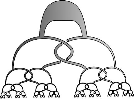
Figure 11. The ball of Alexander $B^{*}$ (final stage)

Theorem 37.

The ball of Alexander $B^{*}$ cannot be an attractor.

Proof.

It is enough to show that $r(B^{*})=\infty$. Begin by writing $B^{*}$ as the union $B^{*}=B^{*}_{1}\cup B^{*}_{2}$ as shown in Figure 12 below. This decomposition is clearly tame. Figure 13 suggests how to prove that both $B^{*}_{1}$ and $B^{*}_{2}$ are ambient homeomorphic to $B^{*}$.

Figure 12. A tame decomposition of $B^{*}$

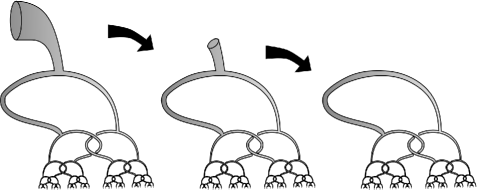
Figure 13. Showing that $B^{*}_{2}$ is ambient homeomorphic to $B^{*}$

We have $r(B^{*})=r(B^{*}_{1})=r(B^{*}_{2})$ by invariance, and also $r(B^{*}_{1})+r(B^{*}_{2})\leq r(B^{*})$ by subadditivity. Therefore

$$2r(B^{*})\leq r(B^{*}),$$

which implies that either $r(B^{*})=0$ or $r(B^{*})=\infty$. Since $B^{*}$ is not cellular, by nullity we have $r(B^{*})\neq 0$. Hence $r(B^{*})=\infty$ and we are finished. ∎

Theorem 37 illustrates again how a perfectly acceptable set, such as a ball, can be embedded in $\mathbb{R}^{3}$ in such a way that it cannot be an attractor.

We stated earlier, while dealing with the subadditivity property, that it does not generally hold for decompositions that are not tame. Now we are in a position to prove this by example.

Example 38.

There is a decomposition of the standard unit ball $K$ into two continua $K_{1}$ and $K_{2}$ that meet in a disk and such that $r(K_{1})+r(K_{2})\not\leq r(K)$. Thus the subadditivity property does not hold for this decomposition.

Proof.

Start with the unit ball $K$. To define $K_{1}$, refer to Figure 14 below and dig a hole in $K$ following the pattern of the ball of Alexander. $K_{2}$ is the part of $K$ that is dug out in this process, that is, $K_{2}:=\overline{K-K_{1}}$. Although $K_{1}$ and $K_{2}$ are shown separately in Figure 14 for clarity purposes, we remark that $K_{2}$ actually fills in the hole in $K_{1}$. Notice that $K_{2}$ is ambient homeomorphic to the ball of Alexander.

Figure 14. A decomposition of $K$ that is not tame

The intersection $K_{1}\cap K_{2}$ is precisely ${\rm fr}\ K_{2}$ (the topological frontier of $K_{2}$) minus the interior of the disk that lies at its top. It is a consequence of the theorem on invariance of domain that ${\rm fr}\ K_{2}$ agrees with the boundary of the manifold $K_{2}$, so ${\rm fr}\ K_{2}$ is a $2$–sphere and consequently $K_{1}\cap K_{2}$ is a $2$–sphere minus a disk, which is again a disk (this follows from the Schönflies’ theorem in the plane).

We have $r(K_{1})\geq 0$ by definition, $r(K)=0$ (this is trivial) and $r(K_{2})=\infty$ by Theorem 37. Therefore

$$\infty=r(K_{1})+r(K_{2})\not\leq r(K)=0$$

and so the subadditivity property does not hold for this decomposition. ∎

8.2. The sphere of Alexander cannot be an attractor

The boundary of the ball of Alexander $B^{*}$ is the sphere of Alexander $S^{*}$. We want to show that $S^{*}$ cannot be an attractor by proving that $r(S^{*})=\infty$.

All the work done so far translates verbatim to compact subsets of $\mathbb{S}^{3}$, rather than $\mathbb{R}^{3}$. Moreover, if $K\subseteq\mathbb{R}^{3}$, then $r(K)$ is the same regardless of whether we consider $K$ as a subset of $\mathbb{R}^{3}$ or $\mathbb{S}^{3}$. Changing our ambient space from $\mathbb{R}^{3}$ to $\mathbb{S}^{3}$ is the most natural setting for what follows.

By a surface we understand a compact $2$–manifold without boundary. When $S\subseteq\mathbb{S}^{3}$ is a connected surface, using Alexander duality and Poincaré duality we have

$$\tilde{H}_{0}(\mathbb{S}^{3}-S)=H^{2}(S)=H_{0}(S)=\mathbb{Z}_{2},$$

so $S$ separates $\mathbb{S}^{3}$ into two complementary domains $U_{1}$ and $U_{2}$. The closures $\overline{U}_{1},\overline{U}_{2}$ are compact subsets of $\mathbb{S}^{3}$, so $r(\overline{U}_{1})$ and $r(\overline{U}_{2})$ are defined. It turns out that there is a very simple relation among these numbers and $r(S)$:

Proposition 39.

Let $S\subseteq\mathbb{S}^{3}$ be a connected surface and $U_{1}$, $U_{2}$ its complementary domains. Then

$$r(S)=r(\overline{U}_{1})+r(\overline{U}_{2}).$$

Before proving this result we need Lemma 40 below. Its proof is an adaptation of an argument contained in the book by Munkres [19, Theorem 36.3, p. 205].

Lemma 40.

Let $U_{1}$ and $U_{2}$ be the complementary domains of a connected surface $S\subseteq\mathbb{S}^{3}$. Then their topological frontiers ${\rm fr}\ U_{1}$ and ${\rm fr}\ U_{2}$ coincide with $S$.

Proof.

The only nontrivial part is to show that ${\rm fr}\ U_{1}$ and ${\rm fr}\ U_{2}$ are not only subsets of $S$, but that they are all of $S$. To prove this, observe first that the compact set $C:={\rm fr}\ U_{1}$ separates $\mathbb{S}^{3}$, for no point $p\in U_{1}$ can be joined to a point $q\in U_{2}$ with a path that does not meet $C$. Thus by Spanier’s version of Alexander duality [28, Theorem 17, p. 296] in $\mathbb{S}^{3}$ we see that $\check{H}^{2}(C)\neq 0$. Again by Alexander duality, but now in the surface $S$, it follows that $H_{0}(S,S-C)=\check{H}^{2}(C)\neq 0$. Since $S$ is connected, this requires that $S-C=\emptyset$, so $C=S$ as we wanted to prove. An analogous argument shows that ${\rm fr}\ U_{2}=C$. ∎

Proof of Proposition 39.

We prove both inequalities.

($\leq$) It will be enough to show that for every neighbourhood $V$ of $S$ there is an $m$–neighbourhood $N$ of $S$ contained in $V$ such that ${\rm rk}\ H_{1}(N)\leq r(\overline{U}_{1})+r(\overline{U}_{2})$.

We assume $r(\overline{U}_{1}),r(\overline{U}_{2})<\infty$, for otherwise there is nothing to prove. Since ${\rm fr}\ \overline{U}_{1}\subseteq S$ is contained in ${\rm int}\ V$, the set $W_{1}:=\overline{U}_{1}\cup V$ is a neighbourhood of $\overline{U}_{1}$. Thus there is an $m$–neighbourhood $N_{1}$ of $\overline{U}_{1}$ such that $N_{1}\subseteq W_{1}$ and ${\rm rk}\ H_{1}(N_{1})=r(\overline{U}_{1})$. Similarly, there is an $m$–neighbourhood $N_{2}$ of $\overline{U}_{2}$ such that $N_{2}\subseteq W_{2}:=\overline{U}_{2}\cup V$ and ${\rm rk}\ H_{1}(N_{2})=r(\overline{U}_{2})$.

Let $N:=N_{1}\cap N_{2}$, which is an $m$–neighbourhood of $S$ contained in $W_{1}\cap W_{2}=V$. Since $\mathbb{S}^{3}=N_{1}\cup N_{2}$, there is a Mayer–Vietoris exact sequence

$$H_{2}(\mathbb{S}^{3})=0\longrightarrow H_{1}(N)\longrightarrow H_{1}(N_{1})\oplus H_{1}(N_{2}),$$

whence ${\rm rk}\ H_{1}(N)\leq{\rm rk}\ H_{1}(N_{1})+{\rm rk}\ H_{1}(N_{2})=r(\overline{U}_{1})+r(\overline{U}_{2})$.

($\geq$) We assume $r(S)<\infty$, for otherwise there is nothing to prove.

Let $V_{1}$ and $V_{2}$ be neighbourhoods of $\overline{U}_{1}$ and $\overline{U}_{2}$ respectively. $\overline{U}_{1}$ and $\overline{U}_{2}$ both contain $S$ by Lemma 40, so $V_{1}\cap V_{2}$ is a neighbourhood of $S$. Thus there exists an $m$–neighbourhood $N$ of $S$ such that $N\subseteq V_{1}\cap V_{2}$ and ${\rm rk}\ H_{1}(N)=r(S)$. Denote $N_{1}:=\overline{U}_{1}\cup N$ and $N_{2}:=\overline{U}_{2}\cup N$. These are $m$–neighbourhoods of $\overline{U}_{1}$ and $\overline{U}_{2}$ respectively. Observe that $N_{1}\cap N_{2}=N$ and $N_{1}\cup N_{2}=\mathbb{S}^{3}$, so from the Mayer–Vietoris sequence

$$H_{1}(N)\longrightarrow H_{1}(N_{1})\oplus H_{1}(N_{2})\longrightarrow H_{1}(\mathbb{S}^{3})=0$$

we see that ${\rm rk}\ H_{1}(N_{1})+{\rm rk}\ H_{1}(N_{2})\leq{\rm rk}\ H_{1}(N)$. Since $N_{1}\subseteq V_{1}$ and $N_{2}\subseteq V_{2}$, we conclude that $r(\overline{U}_{1})+r(\overline{U}_{2})\leq r(S)$. ∎

Theorem 41.

The sphere of Alexander $S^{*}$ cannot be an attractor.

Proof.

The closure of one of the complementary domains of $S^{*}$ is precisely the ball of Alexander $B^{*}$. From Theorem 37 we know $r(B^{*})=\infty$, and then Proposition 39 implies $r(S^{*})\geq r(B^{*})=\infty$. ∎

9. Comparing $r(K)$ and Čech cohomology

The definition of $r(K)$ suggests that $r(K)$ encodes two different pieces of information about $K$: it captures its “intrinsic complexity” as measured by ${\rm rk}\ \check{H}^{1}(K)$ and, in addition, it includes an extra term that accounts for the “crookedness” of $K$ as a subset of $\mathbb{R}^{3}$. On these intuitive grounds we may expect the inequality $r(K)\geq{\rm rk}\ \check{H}^{1}(K)$ to hold true, and this is actually the case:

Theorem 42.

Let $K$ be a compact subset of $\mathbb{R}^{3}$. Then $r(K)\geq{\rm rk}\ \check{H}^{1}(K)$.

The proof of this inequality depends on Lemma 43 below, which is an easy algebraic result. However, it should be noted that it makes essential use (for the only time in this paper) of the fact that we are computing homologies and cohomologies with coefficients in a field and therefore the homology and cohomology groups are actually vector spaces. Recall that the dimension of a vector space $V$ agrees with its rank when viewed as an abelian additive group.

Lemma 43.

Let

$$V_{1}\stackrel{{\scriptstyle\varphi_{1}}}{{\longrightarrow}}V_{2}\stackrel{{\scriptstyle\varphi_{2}}}{{\longrightarrow}}\ldots\stackrel{{\scriptstyle\varphi_{k-1}}}{{\longrightarrow}}V_{k}\stackrel{{\scriptstyle\varphi_{k}}}{{\longrightarrow}}\ldots$$

be a direct sequence of vector spaces and let $V$ be its direct limit. If ${\rm dim}\ V_{k}\leq r<\infty$ for every $k$, then ${\rm dim}\ V\leq r$.

Proof.

By the definition of direct limit, each $v\in V$ is of the form $\psi_{k}(u_{k})$ for suitable $k$ and $u_{k}\in V_{k}$. It is an easy exercise to see that this holds more generally: if $S\subseteq V$ is finite, then $S=\psi_{k}(U)$ for suitable $k$ and $U\subseteq V_{k}$.

Now suppose that ${\rm dim}\ V>r$, so there exists a linearly independent set $S\subseteq V$ with $r+1$ elements. Then $S=\psi_{k}(U)$ for suitable $k$ and $U\subseteq V_{k}$, and $U$ must contain at least $r+1$ linearly independent elements. This contradicts the hypothesis that ${\rm dim}\ V_{k}\leq r$. ∎

Proof of Theorem 42.

If $r(K)=\infty$ there is nothing to prove, so we assume that $r(K)=r<\infty$. By Proposition 11.ii $K$ has a $pm$–neighbourhood basis $\{N_{k}\}$ such that ${\rm rk}\ H_{1}(N_{k})=r$ for every $k$, which implies ${\rm rk}\ H^{1}(N_{k})=r$ by the universal coefficient theorem. We may as well assume that $N_{k+1}\subseteq N_{k}$ for each $k$, and then by the continuity property of Čech cohomology $\check{H}^{1}(K)$ is the direct limit of the sequence

$$H^{1}(N_{1})\longrightarrow H^{1}(N_{2})\longrightarrow H^{1}(N_{2})\longrightarrow\ldots$$

where the bonding maps are induced by inclusions. Then Lemma 43 implies that ${\rm rk}\ \check{H}^{1}(K)\leq r=r(K)$. ∎

Of course, the inequality in Theorem 42 may be strict: the nonattracting arcs, balls and spheres constructed earlier all have trivial $\check{H}^{1}$ and infinite $r$. When ${\rm rk}\ \check{H}^{1}(K)<\infty$ it will be convenient to denote $c(K)$ the nonnegative integer, possibly $\infty$, such that

$$r(K)={\rm rk}\ \check{H}^{1}(K)+c(K).$$

We shall accept that $c(K)$ quantifies the “crookedness” of $K$ as a subset of $\mathbb{R}^{3}$ much in the same way as $r(K)$ does, but having factored out the contribution due to the “intrinsic complexity” of $K$. Clearly $c$ inherits from $r$ both the invariance and the finiteness properties.

It is natural to expect that polyhedra should have $c=0$. This turns out to be true:

Proposition 44.

Let $K\subseteq\mathbb{R}^{3}$ be a polyhedron. Then $c(K)=0$.

Proof.

It is well known that ${\rm rk}\ \check{H}^{1}(K)={\rm rk}\ H^{1}(K)<\infty$ for a poyhedron, so $c(K)$ is defined. Let $\{N_{k}\}$ be a $pm$–neighbourhood basis of $K$ whose members are all regular neighbourhoods of $K$. Each inclusion $K\subseteq N_{k}$ is a homotopy equivalence so ${\rm rk}\ \check{H}^{1}(N_{k})={\rm rk}\ \check{H}^{1}(K)$ for every $k$, which easily implies $r(K)\leq{\rm rk}\ \check{H}^{1}(K)$. Together with Theorem 42 this shows that $r(K)={\rm rk}\ \check{H}^{1}(K)$ and $c(K)=0$. ∎

Another interesting class of sets for which $c=0$ is that of attractors for flows.

Proposition 45.

Let $K\subseteq\mathbb{R}^{3}$ be an attractor for a flow. Then $c(K)=0$.

Proof.

Since $K$ is also an attractor for the time-one map of the flow, by the finiteness property $r(K)<\infty$ so $c(K)$ is defined. $K$ has arbitrarily small $m$–neighbourhoods $P$ such that the inclusion $K\subseteq P$ induces isomorphisms in Cech cohomology [26, Proposition 6 and Remark 9, p. 6168] which implies $r(K)\leq{\rm rk}\ \check{H}^{1}(K)$. Together with Theorem 42 this proves that $c(K)=0$. ∎

Proposition 45 can be used to show that certain sets which are attractors for homeomorphisms cannot be attractors for flows. This is the case of the dyadic solenoid and the Whitehead continuum, as we now describe.

The dyadic solenoid. Let $T\subseteq\mathbb{R}^{3}$ be a solid torus, and let $f:\mathbb{R}^{3}\longrightarrow\mathbb{R}^{3}$ be a homeomorphism such that $f(T)$ winds twice inside $T$ as shown in Figure 15. The set $K:=\bigcap_{k}f^{k}(T)$ is known as the dyadic solenoid, and it is an attractor for $f$ by its very construction.

Figure 15. Constructing the dyadic solenoid

Example 46.

The dyadic solenoid $K$ has $c(K)=1$. Thus by Proposition 45 it cannot be an attractor for a flow, although it is an attractor for a homeomorphism.

Proof.

For each $k$ let $N_{k}$ be the solid torus $f_{k}(T)$. Clearly $\{N_{k}\}$ is an $m$–neighbourhood basis of $K$, so $r(K)\leq 1$ because ${\rm rk}\ H_{1}(N_{k})=1$ for every $k$. Using the continuity property of Čech cohomology it is very easy to see that $\check{H}^{d}(K;\mathbb{Z}_{2})=0$ for every $d\geq 1$ but $\check{H}^{1}(K;\mathbb{Z})\neq 0$. The latter implies that $K$ is not cellular, and then by the nullity property $r(K)\geq 1$. It follows that $r(K)=1$ and $c(K)=1$ too. ∎

The Whitehead continuum. Let $T\subseteq\mathbb{R}^{3}$ be a solid torus, and let $f:\mathbb{R}^{3}\longrightarrow\mathbb{R}^{3}$ be a homeomorphism such that $f(T)$ lies inside $T$ as shown in Figure 16. The set $K:=\bigcap_{k}f^{k}(T)$ is known as the Whitehead continuum, and it is an attractor for $f$ by its very construction.

Figure 16. Constructing the Whitehead continuum

Example 47.

The Whitehead continuum $K$ has $c(K)=1$. Thus by Proposition 45 it cannot be an attractor for a flow, although it is an attractor for a homeomorphism.

Proof.

As in Example 46, $r(K)\leq 1$. Each torus $f^{k+1}(T)$ is nullhomotopic inside the previous one $f^{k}(T)$, so $\check{H}^{d}(K;\mathbb{Z})=0$ for every $d\geq 1$. The Whitehead continuum is not cellular [14, p. 156], so by the nullity property $r(K)=1$. Thus $c(K)=1$. ∎

If the reader is familiar with shape theory [3] he may want to consider the following remark. There is a result of Günther and Segal [11, Corollary 1, p. 324] which states that every attractor for a flow on a manifold has the shape of a (finite) polyhedron, so in particular it has finitely generated Čech cohomology in every dimension and for every coefficient group (this holds true even if attractors are allowed to be mildly unstable [18, 25]). Since the dyadic solenoid has nonfinitely generated $\check{H}^{1}(K;\mathbb{Z})$, it follows that it cannot be an attractor for a flow [11, Example 3, p. 325] which agrees with Example 46. Conversely, Günther and Segal also show that a (finite dimensional, metrizable) compact set having the shape of a finite polyhedron can be embedded in some Euclidean space in such a way that it is an attractor for a suitable flow [11, Theorem 2, p. 327]. The Whitehead continuum does have the shape of a finite polyhedron (it has the shape of a point), but according to Example 47 it cannot be an attractor in $\mathbb{R}^{3}$. However, if $K$ is thought of as a subset of $\mathbb{R}^{4}$ (identifying $\mathbb{R}^{3}$ with $\mathbb{R}^{3}\times\{0\}\subseteq\mathbb{R}^{4}$) then it becomes cellular and it is an attractor for a suitable flow in $\mathbb{R}^{4}$. This shows how shape theory, which is a topological invariant and cannot discriminate between $K\subseteq\mathbb{R}^{3}$ and $K\subseteq\mathbb{R}^{4}$, cannot be used to analyse Example 47.

10. Final remarks and open questions

We finish this paper by stating some open questions.

10.1.

Of course,

Question 1. Solve the characterization problem for $M=\mathbb{R}^{3}$.

or even more ambitiously, solve the characterization problem when the dynamics on the attractor is given:

Question 2. Assume $K\subseteq\mathbb{R}^{3}$ is a compact set on which a homeomorphism $h:K\longrightarrow K$ is defined. Characterize when it is possible to extend $h$ to a homeomorphism $\hat{h}:\mathbb{R}^{3}\longrightarrow\mathbb{R}^{3}$ having $K$ as an attractor.

There is a very interesting situation, related to the theory of partial differential equations (PDEs), in which this question arises naturally. A PDE generates a flow or semiflow on an infinite-dimensional phase space, but many of them (especially those with a physical motivation) have finite-dimensional attractors. A copy $K$ of such an attractor can be embedded together with its dynamics in some finite dimensional Euclidean space $E$, and the question arises whether there exists a flow in $E$ having $K$ as an attractor and reproducing its dynamics. This can be considered a “parametric version” of the extension problem posed above (with $\mathbb{R}^{3}$ replaced by $E$). Heuristically, if such a flow exists then a finite number of variables suffices to describe completely the long term behaviour of the original system modelled by the PDE. The question was first studied by Eden, Foias, Nicolaenko and Temam [7] as well as Romanov [23] but only later [20, 21, 22] it was noticed that the way $K$ is embedded in $E$ needs to be carefully controlled; it also became clear that the mathematical language needed to describe how $K$ should sit in $E$ is still to be developed. We hope that the ideas introduced in the present paper provide a starting point for this task.

10.2.

Suppose $K$ is an attractor for $f$. Let $N\subseteq\mathcal{A}(K)$ be an $m$–neighbourhood of $K$. Since $K$ attracts $N$, there exists $n_{0}\in\mathbb{N}$ such that $f^{n_{0}}(N)\subseteq{\rm int}\ N$. Letting $N_{k}:=f^{kn_{0}}(N)$ we obtain (as in Lemma 12) a decreasing $m$–neighbourhood basis of $K$ all of whose members are homeomorphic to each other, but with the additional property that $f^{k}$ provides a homeomorphism from the pair $(N_{0},N_{1})$ onto the pair $(N_{k},N_{k+1})$. Less technically stated, $\{N_{k}\}$ has the property that each $N_{k+1}$ lies in $N_{k}$ in the same way as $N_{1}$ lies in $N_{0}$.

Question 3. Is it possible to refine the definition of $r(K)$ in such a way that it accounts for the above observation?

Let us include a specific example to illustrate this question. Denote $\nu_{k}$ the sequence of prime numbers $2,3,5,7,11,13,\ldots$ Consider a solid torus $T_{0}\subseteq\mathbb{R}^{3}$. Place in its interior another solid torus $T_{1}$ that winds $\nu_{1}=2$ times around $T_{0}$. Then place in the interior of $T_{1}$ another solid torus $T_{2}$ that winds $\nu_{2}=3$ times around $T_{1}$, and so on. Repeating this construction one obtains a nested sequence of tori $\{T_{k}\}$, each winding $\nu_{k}$ times around the previous one, whose intersection is a compact set $K$. Clearly $r(K)\leq 1<\infty$, so $r$ does not rule out the possibility that $K$ is an attractor, but our intuition tells us that it cannot because there is no repeating pattern in how each $T_{k+1}$ lies in the previous $T_{k}$. A beautiful result of Günther [10, Theorem 1, p. 653] confirms this intuition by an ingenious examination of the structure of $\check{H}^{1}(K;\mathbb{Z})$.

10.3.

Throughout the paper we have concentrated on discrete dynamical systems, but the characterization problem makes perfect sense also in the context of continuous dynamical systems: “characterize topologically what compact sets $K\subseteq\mathbb{R}^{3}$ can be attractors for flows on $\mathbb{R}^{3}$”. Being an attractor for a flow is much more restrictive than being an attractor for a homeomorphism (Examples 46 and 47 illustrate this), which makes this version of the characterization problem easier to deal with. It can be answered in the following terms:

Theorem. [26, Theorem 11, p. 6169] A compactum $K\subseteq\mathbb{R}^{3}$ is an attractor for a flow if and only if there exists a polyhedron $P\subseteq\mathbb{R}^{3}$ such that $\mathbb{S}^{3}-K$ is homeomorphic to $\mathbb{S}^{3}-P$.

The interesting point to be observed here is that whether $K$ is an attractor for a flow depends only on $\mathbb{S}^{3}-K$.

Question 4. Suppose $K,K^{\prime}\subseteq\mathbb{R}^{3}$ are compacta such that $\mathbb{S}^{3}-K$ and $\mathbb{S}^{3}-K^{\prime}$ are homeomorphic. Is it true that if $K$ is an attractor for a homeomorphism, then so must be $K^{\prime}$?

If the answer to this question is negative (that is, if there exist compacta with homeomorphic complements in $\mathbb{S}^{3}$, one being an attractor and the other one not) then the characterization problem cannot be solved in terms of invariants such as $r(K)$, for we saw earlier that these depend only on $\mathbb{S}^{3}-K$ (Theorem 15).

10.4.

If the reader is acquainted with the notions of wild and tame sets from geometric topology he might have been reminded of them by the overall flavour of the paper. Recall that a compact set $K\subseteq\mathbb{R}^{3}$ is called tame if there exist a polyhedron $P\subseteq\mathbb{R}^{3}$ and a homeomorphism $h:\mathbb{R}^{3}\longrightarrow\mathbb{R}^{3}$ such that $h(K)=P$; otherwise $K$ is said to be wild. It is almost unavoidable to wonder whether there is some relation between these concepts and the characterization problem. One has the following result:

Proposition. [26, Proposition 12, p. 6169] Every tame set is an attractor for a flow; hence also for a homeomorphism (namely, the time-one map of the flow).

This was essentially proved by Günther and Segal [11, Corollary 4, p. 327]. It explains why all our examples of nonattracting sets are wild, although one should not be misled to think that no wild set can be an attractor: for instance, the dyadic solenoid is wild but it is an attractor, and it is even possible to construct wild arcs that are attractors [26, Example 38, p. 6177].

The notions of tameness and wildness have local versions when applied to arcs or spheres. An arc $A\subseteq\mathbb{R}^{3}$ is locally tame at a point $p\in A$ if there exist a neighbourhood $U$ of $p$ in $\mathbb{R}^{3}$ and a homeomorphism $h:\mathbb{R}^{3}\longrightarrow\mathbb{R}^{3}$ such that $h(U\cap A)$ is contained in the $x$–axis. Similarly, a sphere $S\subseteq\mathbb{R}^{3}$ is locally tame at a point $p\in S$ if there exist a neighbourhood $U$ of $p$ in $\mathbb{R}^{3}$ and a homeomorphism $h:\mathbb{R}^{3}\longrightarrow\mathbb{R}^{3}$ such that $h(U\cap S)$ is contained in the $xy$–plane. In both cases, the set of points at which the given set $K$ is tame is an open subset of $K$; its complement is a compact subset of $K$ called the wild set of $K$.

Question 5. Is it possible to characterize when an arc or a sphere is an attractor in terms of properties of their wild sets?

10.5.

We used the Fox–Artin arc $F$ shown in Figure 2 as a basis for our construction of an arc that cannot be an attractor. It is fairly easy to construct a neighbourhood basis of $F$ comprised of double tori, so $r(F)\leq 2$. We also know that $r(F)\geq 1$ because $F$ is not cellular.

Question 6. What is $r(F)$? Can $F$ be an attractor?

Appendix: Alexander duality for manifolds with boundary

Lemma 48.

Let $N$ be a compact $3$–manifold and $S\subseteq{\rm int}\ N$ a compact set. Then $H_{d}(N,S)=H_{3-d}(N-S,\partial N)$.

Proof.

$\partial N$ is collared in $N$ [5]. This means that there exists an embedding $c:\partial N\times[0,1]\longrightarrow N$ such that $c(p,0)=p$ for every $p\in\partial N$. Since $S$ is a compact subset of ${\rm int}\ N$, there exists $\varepsilon>0$ such that $c(\partial N\times[0,\varepsilon])$ is disjoint from $S$. The theorem on invariance of domain guarantees that $U:=c(\partial N\times[0,\varepsilon))$ is an open subset of $N$, and it is not difficult to check that $N^{*}:=N-U$ is a compact $3$–manifold contained in ${\rm int}\ N$ and containing $S$ in its interior. The inclusions $N^{*}\subseteq N$ and $\partial N\subseteq N-N^{*}$ are both homotopy equivalences.

The cohomology exact sequence for the triple $(N,N^{*},S)$ and the fact that $\check{H}^{*}(N,N^{*})=0$ imply that $\check{H}^{d}(N,S)=\check{H}^{d}(N^{*},S)$. Using Spanier’s version of Alexander duality [28, Theorem 17, p. 296] for the compact pair $(N^{*},S)$ in the interior of the boundariless manifold ${\rm int}\ N$ we have

$$\check{H}^{d}(N^{*},S)=H_{3-d}(({\rm int}\ N)-S,({\rm int}\ N)-N^{*}).$$

An easy exercise involving the collar $c$ shows that $H_{3-d}(({\rm int}\ N)-S,({\rm int}\ N)-N^{*})=H_{3-d}(N-S,N-N^{*})$ so

$$\check{H}^{d}(N^{*},S)=H_{3-d}(N-S,N-N^{*}),$$

which readily implies that

$$\check{H}^{d}(N,S)=H_{3-d}(N-S,\partial N).$$

∎

References

- [1] J. W. Alexander. An example of a simply connected surface bounding a region which is not simply connected. Proc. Nat. Acad. Sci. U.S.A., 10:8–10, 1924.
- [2] W. A. Blankinship and R. H. Fox. Remarks on certain pathological open subsets of –space and their fundamental groups. Proc. Amer. Math. Soc., 1(5):618–624, 1950.
- [3] K. Borsuk. Theory of shape. Monografie Matematyczne, Tom 59. Państwowe Wydawnictwo Naukowe, 1975.
- [4] M. Brown. Locally flat imbeddings of topological manifolds. Ann. Math., 75(2):331–341, 1962.
- [5] R. Connelly. A new proof of Brown’s collaring theorem. Proc. Amer. Math. Soc., 27(1):180–182, 1971.
- [6] R. J. Daverman. Decompositions of manifolds. Pure and Applied Mathematics, 124. Academic Press, 1986.
- [7] A. Eden, C. Foias, B. Nicolaenko, and R. Temam. Exponential attractors for dissipative evolution equations. Wiley, New York, 1994.
- [8] R. H. Fox and E. Artin. Some wild cells and spheres in three-dimensional space. Ann. Math. (2), 49(4):979–990, 1948.
- [9] B. M. Garay. Strong cellularity and global asymptotic stability. Fund. Math., 138:147–154, 1991.
- [10] B. Günther. A compactum that cannot be an attractor of a self-map on a manifold. Proc. Amer. Math. Soc., 120(2):653–655, 1994.
- [11] B. Günther and J. Segal. Every attractor of a flow on a manifold has the shape of a finite polyhedron. Proc. Amer. Math. Soc., 119(1):321–329, 1993.
- [12] J. K. Hale. Asymptotic behaviour of dissipative systems. American Mathematical Society, 1988.
- [13] A. Hatcher. Algebraic topology. Cambridge University Press, 2002.
- [14] J. Hempel. 3-manifolds. Princeton University Press, 1976.
- [15] J. F. P. Hudson. Piecewise linear topology. W. A. Benjamin, Inc., 1969.
- [16] A. Katok and B. Hasselblatt. Introduction to the modern theory of dynamical systems. Cambridge University Press, 1996.
- [17] E. E. Moise. Geometric topology in dimensions 2 and 3. Springer-Verlag, 1977.
- [18] M. A. Morón, J. J. Sánchez-Gabites, and J. M. R. Sanjurjo. Topology and dynamics of unstable attractors. Fund. Math., 197:239–252, 2007.
- [19] J. Munkres. Elements of algebraic topology. Addison–Wesley Publishing Company, Inc., 1984.
- [20] E. Pinto de Moura, J. C. Robinson, and J .J. Sánchez-Gabites. Embedding of global attractors and their dynamics. Proc. Amer. Math. Soc., 139(10):3497–3512, 2011.
- [21] J. C. Robinson. Global attractors: Topology and finite-dimensional dynamics. J. Dynam. Differential Equations, 11(3):557–581, 1999.
- [22] J. C. Robinson and J. J. Sánchez-Gabites. On finite-dimensional attractors of homeomorphisms. 2013. Preprint.
- [23] A. V. Romanov. Finite-dimensional limiting dynamics for dissipative parabolic equations. Sb. Math., 191:415–429, 2000.
- [24] J. J. Sánchez-Gabites. On the shape of attractors for discrete dynamical systems. 2010. Preprint.
- [25] J. J. Sánchez-Gabites. Unstable attractors in manifolds. Trans. Amer. Math. Soc., 362(7):3563–3589, 2010.
- [26] J. J. Sánchez-Gabites. How strange can an attractor for a dynamical system in a -manifold look? Nonlinear Anal., (74):6162–6185, 2011.
- [27] C. D. Sikkema. A duality between certain spheres and arcs in . Trans. Amer. Math. Soc., 122(2):399–415, 1966.
- [28] E. H. Spanier. Algebraic topology. McGraw–Hill Book Co., 1966.