Fully Automated Calculations in the complex MSSM

Abstract:

We review recent progress towards automated higher-order calculations in the MSSM with complex parameters (cMSSM). The consistent renormalization of all relevant sectors of the cMSSM and the inclusion into the FeynArts/FormCalc framework has recently been completed. Some example calculations applying this framework are briefly discussed. These include two-loop corrections to cMSSM Higgs boson masses as well as partial decay widths of electroweak supersymmetric particles decaying into a Higgs boson and another supersymmetric particle.

1 Introduction

Two of the most important goals of the experiments at the Large Hadron Collider (LHC) are to identify the origin of electroweak symmetry breaking (EWSB), and to search for physics effects beyond the Standard Model (SM). The spectacular discovery of a Higgs-like particle with a mass around $\sim 125.6\,\,\mathrm{GeV}$, which was announced by ATLAS and CMS [1, 2], marks a milestone of an effort that has been ongoing for almost half a century and opens a new era of particle physics. Within the experimental uncertainties the properties of the newly discovered particle are in agreement with the predictions of the SM Higgs boson [3, 4]. However, the uncertainties still leave room for contributions from non-SM degrees of freedom, see, e.g., Refs. [5, 6, 7] for a recent combination and reviews. The prime task now is to study the properties of the discovered new particle in detail and to investigate whether there are significant deviations from the SM predictions, which would point towards physics beyond the SM.

The extent to which the results of the Higgs searches at the LHC can discriminate between the SM and possible alternatives depends both on the experimental precision with which the properties of a possible signal can be determined and on the detailed nature of the mechanism for EWSB that is actually realized in nature. One of the leading candidates for physics beyond the SM (BSM) is supersymmetry (SUSY), which doubles the particle degrees of freedom by predicting two scalar partners for all SM fermions, as well as fermionic partners to all bosons. The most widely studied SUSY framework is the Minimal Supersymmetric Standard Model (MSSM) [8], which keeps the number of new fields and couplings to a minimum. The MSSM Higgs sector contains two Higgs doublets, which at the tree-level leads to a physical spectrum consisting of two ${\cal CP}$-even, $h,H$, one ${\cal CP}$-odd, $A$, and two charged Higgs bosons, $H^{\pm}$.

In order to investigate the impact of the Higgs search results at the LHC on possible scenarios of new physics, precise theoretical predictions both within the SM and possible alternatives of it are needed. In particular, if small deviations from the SM predictions are probed it is crucial to treat the considered model of new physics at the same level of precision to enable an accurate analysis and comparison. In the MSSM Higgs sector higher-order contributions are known to give numerically large effects (see, e.g., Refs. [9, 10]). For many observables it is therefore necessary to include corrections beyond leading order in the perturbative expansion to obtain reliable results. The calculation of loop diagrams, often involving a large number of fields, is a tedious and error-prone task if done by hand. This is true in particular for BSM theories where the number of fields is significantly increased. For one-loop calculations, as will be the focus in the following, computer methods with a high degree of automatization have been devised to simplify the work. However, most of the available tools so far have focused on calculations either in the SM or the MSSM with external SM particles.

Here we review renormalization of the MSSM including complex parameters (cMSSM) and the corresponding implementation as a model file [11] into the FeynArts [12, 13]/FormCalc [14] framework. This implementation allows for automated calculation of processes with external SUSY particles. We also briefly discuss the application of the new FeynArts model file to the calculation of two-loop corrections to cMSSM Higgs boson masses [15, 16], and to the evaluation of partial decay widths of SUSY electroweak (EW) particles [17, 18, 19].

2 Renormalization of the cMSSM

The tree-level Feynman rules of the MSSM are by now well under control, where the cMSSM had been included into the FeynArts package [13]. Concerning the renormalization, however, most calculations in the past chose a prescription that was tailored to one specific calculation or even one specific part of the (c)MSSM parameter space. Since the values of the SUSY parameters realized in nature are unknown, at the current state scans over large parts of the cMSSM parameter space are necessary. Furthermore, many processes have to be evaluated simultaneously. Both requirements make a complete renormalization of the cMSSM necessary that is valid over the full (or at least “large parts”) of the cMSSM parameter space. Only with such a renormalization at hand fully automated calculations in the cMSSM will be possible. Evidently, calculations at $n$-loop require an $n$-loop renormalization, where we will focus on the one-loop case.

The program of the renormalization of all (physical) sectors of the cMSSM has recently been completed [20, 21, 22, 23, 24, 17, 18, 19, 11] (based on earlier work in the MSSM [25, 26, 27, 28]; for alternative approaches see Refs. [29, 30, 31]) and included as a model file MSSMCT.mod [11] into the FeynArts package.

In the development of the renormalization particular emphasis was put on the requirement that the one-loop corrections stay “small” over the full allowed parameter range. The renormalization includes the scalar fermion sector, the remaining colored sector, the chargino/neutralino sector and the Higgs sector (as well as the SM part of the MSSM). In principle this is sufficient to evaluate all currently relevant processes at the one-loop level. Extensive checks have been performed to ensure “stability” of the higher-order corrections over large(st) parts of the cMSSM parameter space. These tests include scalar top and bottom decays [21, 22], scalar tau decays [24], gluino decays [23] as well as non-hadronic chargino [17] and neutralino decays [18, 19]. These evaluations are complete at the one-loop level, including hard and soft QED and QCD radiation.

leptons	$f=f^{\dagger}\!$	field	mass	sleptons	$f=f^{\dagger}\!$	field	mass
$\nu_{g}$		F[1, {$\mathit{g}$}]	0	$\tilde{\nu}_{g}$		S[11, {$\mathit{g}$}]	MSf
$\ell_{g}$		F[2, {$\mathit{g}$}]	MLE	$\tilde{\ell}_{g}^{s}$		S[12, {$\mathit{s}$,$\mathit{g}$}]	MSf
quarks				squarks
$u_{g}$		F[3, {$\mathit{g}$,$\mathit{o}$}]	MQU	$\tilde{u}_{g}^{s}$		S[13, {$\mathit{s}$,$\mathit{g}$,$\mathit{o}$}]	MSf
$d_{g}$		F[4, {$\mathit{g}$,$\mathit{o}$}]	MQD	$\tilde{d}_{g}^{s}$		S[14, {$\mathit{s}$,$\mathit{g}$,$\mathit{o}$}]	MSf
gauge bosons				neutralinos, charginos
$\gamma$	yes	V[1]	0	$\tilde{\chi}_{n}^{0}$	yes	F[11, {$\mathit{n}$}]	MNeu
$Z$	yes	V[2]	MZ	$\tilde{\chi}_{c}^{-}$		F[12, {$\mathit{c}$}]	MCha
$W^{-}$		V[3]	MW
Higgs/Goldstone bosons				ghosts
$h$	yes	S[1]	Mh0	$u_{\gamma}$		U[1]	0
$H$	yes	S[2]	MHH	$u_{Z}$		U[2]	MZ
$A$	yes	S[3]	MA0	$u_{+}$		U[3]	MW
$G$	yes	S[4]	MZ	$u_{-}$		U[4]	MW
$H^{-}$		S[5]	MHp	$u_{g}$		U[5, {$\mathit{u}$}]	0
$G^{-}$		S[6]	MW
gluon				gluino
$g$	yes	V[5, {$\mathit{u}$}]	0	$\tilde{g}$	yes	F[15, {$\mathit{u}$}]	MGl

Table 1: The particle content of MSSMCT.mod.

$$\mathit{g} =\texttt{Index[Generation]} =1\dots 3\,,$$

$$\mathit{o} =\texttt{Index[Colour]} =1\dots 3\,,$$

$$\mathit{u} =\texttt{Index[Gluon]} =1\dots 8\,,$$

$$\mathit{s} =\texttt{Index[Sfermion]} =1\dots 2\,,$$

$$\mathit{n} =\texttt{Index[Neutralino]} =1\dots 4\,,$$

$$\mathit{c} =\texttt{Index[Chargino]} =1\dots 2\,.$$

(S)fermions are indexed by    

$$t=\begin{cases}1&\text{(s)neutrinos},\\ 2&\text{charged (s)leptons},\\ 3&\text{up-type (s)quarks},\\ 4&\text{down-type (s)quarks}.\end{cases}$$

Table 2: Index labels and ranges used in MSSMCT.mod.

Mh0, MHH, MA0, MHp	Higgs masses $M_{h}$, $M_{H}$, $M_{A}$, $M_{H^{\pm}}$
Mh0tree, MHHtree, MA0tree, MHptree	tree-level Higgs masses
TB, CB, SB, C2B, S2B	$\tan\beta$, $\cos\beta$, $\sin\beta$, $\cos 2\beta$, $\sin 2\beta$
CA, SA, C2A, S2A	$\cos\alpha$, $\sin\alpha$, $\cos 2\alpha$, $\sin 2\alpha$ (tree-level $\alpha$)
CAB, SAB, CBA, SBA	$\cos(\alpha+\beta)$, $\sin(\alpha+\beta)$, $\cos(\beta-\alpha)$, $\sin(\beta-\alpha)$
MUE	Higgs-doublet mixing parameter $\mu$
MGl	gluino mass $m_{\tilde{g}}$
SqrtEGl	root of the gluino phase, $\mathrm{e}^{\mathrm{i}\varphi_{{\tilde{g}}}/2}$
MNeu[$\mathit{n}$]	neutralino masses $m_{\tilde{\chi}_{n}^{0}}$
ZNeu[$\mathit{n}$, $\mathit{n^{\prime}}$]	neutralino mixing matrix $\mathbf{N}_{nn^{\prime}}$
MCha[$\mathit{c}$]	chargino masses $m_{\tilde{\chi}_{c}^{\pm}}$
UCha[$\mathit{c}$, $\mathit{c^{\prime}}$], VCha[$\mathit{c}$, $\mathit{c^{\prime}}$]	chargino mixing matrices $\mathbf{U}_{cc^{\prime}},\mathbf{V}_{cc^{\prime}}$
MSf[$\mathit{s}$, $\mathit{t}$, $\mathit{g}$]	sfermion masses $m_{{\tilde{f}}_{t,sg}}$
USf[$\mathit{t}$, $\mathit{g}$][$\mathit{s}$, $\mathit{s^{\prime}}$]	sfermion mixing matrix $U^{{\tilde{f}}_{tg}}_{ss^{\prime}}$
Af[$\mathit{t}$, $\mathit{g}$, $\mathit{g^{\prime}}$]	soft-breaking trilinear $A$-parameters $\bigl{(}\mathbf{A}_{f_{t}}\bigr{)}_{gg^{\prime}}$
MW, MZ	gauge-boson masses $M_{W}$, $M_{Z}$
Mf[$\mathit{t}$,$\mathit{g}$]	fermion masses $m_{f_{tg}}$
CW, SW	$c_{\mathrm{w}}\equiv\cos\theta_{\text{w}}=M_{W}/M_{Z}$, $s_{\mathrm{w}}\equiv\sin\theta_{\text{w}}$
EL	electromagnetic coupling constant $e$
GS	strong coupling constant $g_{s}$

Table 3: Symbols representing the SM and MSSM parameters in MSSMCT.mod.

To give an idea about the new model file we briefly review the various masses, coupling constants etc. as well as the respective counterterms implemented into MSSMCT.mod (all details can be found in Ref. [11]). In Tab. 1 we list the particle content of the model file, where the respective index ranges are given in Tab. 2. The symbols for the masses of the particles, for couplings and mixing angles are shown in Tab. 3. Within the Higgs boson sector the tree-level masses are taken distinct from the higher-order corrected masses (which can be obtained via the automatic link to FeynHiggs [32, 33, 34, 20, 35]). $\tan\beta$ denotes the ratio of the two vacuum expectation values, and $\alpha$ is the angle that diagonalizes the (tree-level) ${\cal CP}$-even Higgs sector. Within the cMSSM all three neutral Higgs bosons can mix to give rise to three ${\cal CP}$-mixed states, $h_{i}$ ($i=1,2,3$). When composing a vertex $\Gamma_{h_{i}}$ from the corresponding tree-level amplitudes $\Gamma_{h}$, $\Gamma_{H}$, and $\Gamma_{A}$, a set of finite $Z$-factors is needed to ensure correct on-shell properties of the external Higgs boson $h_{i}$ [20],

$$\Gamma_{h_{i}}=\hat{Z}_{i1}\Gamma_{h}+\hat{Z}_{i2}\Gamma_{H}+\hat{Z}_{i3}\Gamma_{A}+\ldots\,,$$ (1)

where the ellipsis represents contributions from the mixing with the Goldstone and $Z$ boson. The $Z$-factor matrix $\hat{Z}_{ij}\equiv\texttt{ZHiggs[$\mathit{i}$,\,$\mathit{j}$]}$ is not in general unitary. Its lower $3\times 3$ part is computed by FeynHiggs and application at the amplitude level automatically takes any absorptive contribution into account. Technically this is most easily accomplished using the FeynArts add-on model file HMix.mod [36] which mixes $h=\texttt{S[1]}$, $H=\texttt{S[2]}$, and $A=\texttt{S[3]}$ into two variants of the loop-corrected states $h_{i}$,

S[0, {$$\mathit{i} =\sum_{j=1}^{3}\texttt{UHiggs[$\mathit{i}$,\,$\mathit{j}$]}~{}\texttt{S[$\mathit{j}$]}\,,$$}] (2a)

S[10, {$$\mathit{i} =\sum_{j=1}^{3}\texttt{ZHiggs[$\mathit{i}$,\,$\mathit{j}$]}~{}\texttt{S[$\mathit{j}$]}\,,$$}] inserted only on external lines. (2b)

Higgs-boson Sector
dZ[bar]Higgs1[$\mathit{h}$, $\mathit{h^{\prime}}$]	Higgs field RCs
dMHiggs1[$\mathit{h}$, $\mathit{h^{\prime}}$]	Higgs mass RCs
dTh01, dTHH1, dTA01	Higgs tadpole RCs
dZH1, dZH2, dTB1, dSB1, dCB1	RCs related to $\beta$
Gauge-boson Sector
dMZsq1, dMWsq1	gauge-boson mass RCs
dZAA1, dZAZ1, dZZA1, dZZZ1, dZ[bar]W1	gauge-boson field RCs
dSW1, dZe1	coupling-constant RCs
Chargino/Neutralino Sector
dMCha1[$\mathit{c}$, $\mathit{c^{\prime}}$]	chargino mass RCs
dMNeu1[$\mathit{n}$, $\mathit{n^{\prime}}$]	neutralino mass RCs
dMino11, dMino21, dMUE1	RCs for $M_{1}$, $M_{2}$, $\mu$
dZ[bar]fLgR1[12, $\mathit{c}$, $\mathit{c^{\prime}}$]	chargino field RCs
dZ[bar]fLgR1[11, $\mathit{n}$, $\mathit{n^{\prime}}$]	neutralino field RCs
Fermion Sector
dMf1[$\mathit{t}$, $\mathit{g}$]	fermion mass RCs
dZ[bar]fLgR1[$\mathit{t}$, $\mathit{g}$, $\mathit{g^{\prime}}$]	fermion field RCs
dCKM1[$\mathit{g}$, $\mathit{g^{\prime}}$]	CKM-matrix RCs
Squark Sector
dMSfsq1[$\mathit{s}$, $\mathit{s^{\prime}}$, 3$|$4, $\mathit{g}$]	squark mass RCs
dAf1[3$|$4, $\mathit{g}$, $\mathit{g}$]	trilinear squark coupling RCs
dZ[bar]SfLgR1[$\mathit{s}$, $\mathit{s^{\prime}}$, 3$|$4, $\mathit{g}$]	squark field RCs
Slepton Sector
dMSfsq1[$\mathit{s}$, $\mathit{s^{\prime}}$, 1$|$2, $\mathit{g}$]	slepton mass RCs
dAf1[2, $\mathit{g}$, $\mathit{g}$]	trilinear slepton coupling RCs
dZ[bar]SfLgR1[$\mathit{s}$, $\mathit{s^{\prime}}$, 1$|$2, $\mathit{g}$]	slepton field RCs
Gluino Sector
dMGl1	gluino mass RC
dZ[bar]GlLgR1	gluino field RCs
Gluon Sector
dZgs1	strong-coupling-constant RC
dZGG1	gluon field RCs

Table 4: RCs used in MSSMCT.mod, where $a$$|$$b$ means ‘$a$ or $b$’ and dZ[bar] stands for both dZ and dZbar (see text).

More details can be found in Refs. [20, 11]. The renormalization constants (RCs) are listed in Tab. 4. For the Higgs boson sector, besides the mass and field renormalization constants also the tadpole counterterms are listed, which correspond to the terms linear in the Higgs fields in the Higgs potential. Several field renormalization constants are given in a barred and unbarred version, differentiating between incoming/outgoing (anti)particles, see Refs. [22, 17, 18, 11] for more details. Several electroweak SM RCs have been omitted (such as dMW1 etc.), since they are defined identical to the pure SM case. The FeynArts/FormCalc framework provides a default implementation of the determination of all RCs, where again the details can be found in Refs. [20, 21, 22, 23, 24, 17, 18, 19, 11]. It should be stressed again that this default implementation is based on the requirement of “stability” of the higher-order corrections over large(st) parts of the cMSSM parameter space.

3 Example applications

In this section we briefly review some of the yet existing applications of MSSMCT.mod.

3.1 Two-loop corrections to Higgs boson masses

Two-loop corrections to cMSSM Higgs boson masses, obtained in the Feynman-diagrammatic approach, require the calculation of two-loop Higgs-boson self-energies, which in turn require a renormalization of the Higgs boson sector at the two-loop level (see Refs. [33, 37, 20, 38, 15, 16, 39]). Furthermore, a sub-loop renormalization of the corresponding one-loop diagrams is necessary. Consequently, a full two-loop calculation of the Higgs-boson self-energies requires a full renormalization of the cMSSM at the one-loop level. Recently, two new two-loop calculations were presented. One consists of the ${\cal O}(\alpha_{t}^{2})$ contributions involving complex phases [16], the other one of the momentum dependent two-loop part of the ${\cal O}(\alpha_{t}\alpha_{s})$ corrections for real parameters [15]. Both types of corrections can yield contributions to $M_{h}$ larger than the current experimental uncertainty. Corresponding one-loop diagrams with sub-loop renormalization are depicted in Fig. 1 (taken from Ref. [15]).

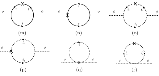
Figure 1: Generic one-loop contributions to cMSSM Higgs-boson self-energies with sub-loop renormalization; $\phi=h,H,A$; $t$ denotes the top quark; ${\tilde{t}}_{i,j}$ the scalar tops with $i,j=1,2$.

3.2 Decays of electroweak SUSY particles

The second example concerns one-loop processes with external SUSY particles. A precise prediction of, e.g., SUSY production cross sections and decay branching ratios is necessary to obtain reliable bounds on the MSSM parameter space from LHC SUSY searches, to correctly interpret any possible signal at the LHC and to exploit the potential of a future $e^{+}e^{-}$ collider such as the ILC, where measurements at the per-cent level will be possible.

Calculations of decay widths of SUSY particles in the cMSSM, using MSSMCT.mod (and its earlier versions) have been published in Refs. [21, 22, 23, 24, 17, 18, 19]. Here we take one representative example from Ref. [18] that involves both a Higgs particle and a Dark Matter particle in the final state, the decay of the fourth neutralino to the lightest neutralino and the lightest Higgs boson, $\tilde{\chi}_{4}^{0}\to\tilde{\chi}_{1}^{0}h_{1}$. The parameters are given in Tab. 5. $M_{2}$ (the $SU(2)$ soft SUSY-breaking parameter) and $\mu$ (the Higgs mixing parameter) are chosen such that the values for $m_{\tilde{\chi}_{1}^{\pm}}$ and $m_{\tilde{\chi}_{2}^{\pm}}$ are fulfilled. Here the ambiguity in the hierarchy of $M_{2}$ and $\mu$ results in two scenarios: $\mu>M_{2}$ yields a higgsino-like $\tilde{\chi}_{4}^{0}$, denoted as ${S}_{h}$; $\mu<M_{2}$ gives a gaugino-like $\tilde{\chi}_{4}^{0}$, denoted as ${S}_{g}$. $|M_{1}|$ (the absolute value of the $U(1)$ soft SUSY-breaking parameter) is obtained from $|M_{1}|=\frac{5}{3}\tan^{2}\theta_{\mathrm{w}}M_{2}\approx\frac{1}{2}M_{2}$, where $\varphi_{M_{1}}$ is kept as a free parameter.

$\tan\beta$	$M_{H^{\pm}}$	$m_{\tilde{\chi}_{2}^{\pm}}$	$m_{\tilde{\chi}_{1}^{\pm}}$	$M_{\tilde{l}_{L}}$	$M_{\tilde{l}_{R}}$	$A_{l}$	$M_{\tilde{q}_{L}}$	$M_{\tilde{q}_{R}}$	$A_{q}$
$20$	$160$	$600$	$350$	$300$	$310$	$400$	$1300$	$1100$	$2000$

Table 5: MSSM parameters with all mass parameters are in$\,\,\mathrm{GeV}$. $M_{H^{\pm}}$ denotes the mass of the charged Higgs boson, $m_{\tilde{\chi}_{1,2}^{\pm}}$ are the chargino masses, $M_{\tilde{l}_{L}}$ and $M_{\tilde{l}_{R}}$ are the diagonal entries in the slepton mass matrices (taken to be universal for the three generations), $A_{l}$ is the trilinear Higgs-slepton coupling; $M_{\tilde{q}_{L}}$, $M_{\tilde{q}_{R}}$ and $A_{q}$ are the corresponding squark sector parameters (see Ref. [18] for details).

The absolute size of $\Gamma(\tilde{\chi}_{4}^{0}\to\tilde{\chi}_{1}^{0}h_{1})$ in ${S}_{g}$ and ${S}_{h}$ is shown in the left plot of Fig. 2 as a function of $\varphi_{M_{1}}$; separately shown are the tree-level results and the full one-loop calculation. A strong dependence of the absolute value of the decay width in both scenarios at the tree-level and at the one-loop level on this phase can be observed. The right plot shows the relative size of the one-loop corrections. Again a strong dependence of the size of those corrections on the phase of $M_{1}$ can be seen. Besides the default implementation of our renormalization scheme, denoted as ${S}_{g}$ and ${S}_{h}$, we also show the results in an alternative on-shell scheme [18, 40] that differs in the treatment of the complex phases, denoted as ${\tilde{S}}_{g}$ and ${\tilde{S}}_{h}$. It can be observed that the two schemes agree for real parameters ($\varphi_{M_{1}}=0,\pi$) and show small differences (indicating the size of respective two-loop corrections) for complex parameters at or below the per-cent level.

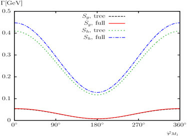
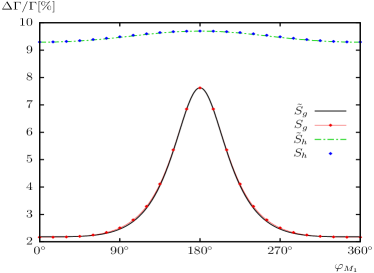
Figure 2: Left: absolute values of $\Gamma(\tilde{\chi}_{4}^{0}\to\tilde{\chi}_{1}^{0}h_{1})$ in the scenarios ${S}_{g}$ and ${S}_{h}$ (see text) at the tree-level and the full one-loop level as a function of $\varphi_{M_{1}}$. Right: relative size of the one-loop corrections in our default renormalization scheme (${S}_{g}$ and ${S}_{h}$) and in an alternative scheme (${\tilde{S}}_{g}$ and ${\tilde{S}}_{h}$, see text) as a function of $\varphi_{M_{1}}$.

Acknowledgements

S.H. thanks the organizers of L&L 2014 for the invitation and the (as always!) inspiring atmosphere, and for being flexible with the talk asignments. We thank A. Bharucha with whom some of the results presented here have been obtained. The work of S.H. is supported in part by the Spanish MICINN’s Consolider-Ingenio 2010 Program under grant MultiDark CSD2009-00064. We furthermore thank the GRID computing network at IFCA for technical help with the OpenStack cloud infrastructure [41], where many of the numerical results shown here have been obtained.

References

- [1] G. Aad et al. [ATLAS Collaboration], Phys. Lett. B 716 (2012) 1 [arXiv:1207.7214 [hep-ex]].
- [2] S. Chatrchyan et al. [CMS Collaboration], Phys. Lett. B 716 (2012) 30 [arXiv:1207.7235 [hep-ex]].
-
[3]
B. Lenzi,
talk given at the LHCP 2014, May 2014, New York, USA,
https://indico.
cern.ch/event/279518/session/1/contribution/54/material/slides/0.pdf ; C. Gwilliam, talk given at the LHCP 2014, May 2014, New York, USA, https://indico.
cern.ch/event/279518/session/1/contribution/56/material/slides/0.pdf . -
[4]
X. Janssen,
talk given at the LHCP 2014, May 2014, New York, USA,
https://indico.
cern.ch/event/279518/session/1/contribution/55/material/slides/0.pdf ; J. Konigsberg, talk given at the LHCP 2014, May 2014, New York, USA, https://indico.
cern.ch/event/279518/session/1/contribution/57/material/slides/0.pdf ; - [5] P. Bechtle, S. Heinemeyer, O. Stål, T. Stefaniak and G. Weiglein, arXiv:1403.1582 [hep-ph].
-
[6]
M. Mühlleitner,
talk given at the LHCP 2014, May 2014, New York, USA,
https://indico.
cern.ch/event/279518/session/17/contribution/19/material/slides/0.pdf . - [7] C. Englert et al., arXiv:1403.7191 [hep-ph].
- [8] H. Nilles, Phys. Rept. 110 (1984) 1; H. Haber and G. Kane, Phys. Rept. 117 (1985) 75; R. Barbieri, Riv. Nuovo Cim. 11 (1988)1.
- [9] A. Djouadi, Phys. Rept. 459 (2008) 1 [arXiv:hep-ph/0503173].
- [10] S. Heinemeyer, Int. J. Mod. Phys. A 21 (2006) 2659 [arXiv:hep-ph/0407244]; S. Heinemeyer, W. Hollik and G. Weiglein, Phys. Rept. 425 (2006) 265 [arXiv:hep-ph/0412214].
-
[11]
T. Fritzsche, T. Hahn, S. Heinemeyer, F. von der
Pahlen, H. Rzehak and C. Schappacher,
Comput. Phys. Commun. 185 1529
[arXiv:1309.1692 [hep-ph]];
T. Hahn et al., these proceedings.
The couplings can be found in the files MSSM.ps.gz, MSSMQCD.ps.gz and HMix.ps.gz as part of the FeynArts package [12]. -
[12]
J. Küblbeck, M. Böhm and A. Denner,
Comput. Phys. Commun. 60 (1990) 165;
A. Denner, H. Eck, O. Hahn and J. Küblbeck, Phys. Lett. B 291 (1992) 278;
A. Denner, H. Eck, O. Hahn and J. Küblbeck, Nucl. Phys. B 387 (1992) 467;
T. Hahn, Comput. Phys. Commun. 140 (2001) 418 [arXiv:hep-ph/0012260]. - [13] T. Hahn and C. Schappacher, Comput. Phys. Commun. 143 (2002) 54 [arXiv:hep-ph/0105349].
- [14] T. Hahn and M. Perez-Victoria, Comput. Phys. Commun. 118 (1999) 153 [arXiv:hep-ph/9807565].
- [15] S. Borowka, T. Hahn, S. Heinemeyer, G. Heinrich and W. Hollik, arXiv:1404.7074 [hep-ph].
- [16] W. Hollik and S. Paßehr, Phys. Lett. B 733 (2014) 144 [arXiv:1401.8275 [hep-ph]].
- [17] S. Heinemeyer, F. von der Pahlen and C. Schappacher, Eur. Phys. J. C 72 (2012) 1892 [arXiv:1112.0760 [hep-ph]]; arXiv:1202.0488 [hep-ph].
- [18] A. Bharucha, S. Heinemeyer, F. von der Pahlen and C. Schappacher, Phys. Rev. D 86 (2012) 075023 [arXiv:1208.4106 [hep-ph]].
- [19] A. Bharucha, S. Heinemeyer and F. von der Pahlen, Eur. Phys. J. C 73 (2013) 2629 [arXiv:1307.4237 [hep-ph]].
- [20] M. Frank, T. Hahn, S. Heinemeyer, W. Hollik, H. Rzehak and G. Weiglein, JHEP 0702 047 (2007) [arXiv:hep-ph/0611326].
- [21] S. Heinemeyer, H. Rzehak and C. Schappacher, Phys. Rev. D 82 (2010) 075010 [arXiv:1007.0689 [hep-ph]]; PoS CHARGED 2010 (2010) 039 [arXiv:1012.4572 [hep-ph]].
- [22] T. Fritzsche, S. Heinemeyer, H. Rzehak and C. Schappacher, Phys. Rev. D 86 (2012) 035014 [arXiv:1111.7289 [hep-ph]]; arXiv:1201.6305 [hep-ph].
- [23] S. Heinemeyer and C. Schappacher, Eur. Phys. J. C 72 (2012) 1905 [arXiv:1112.2830 [hep-ph]].
- [24] S. Heinemeyer and C. Schappacher, Eur. Phys. J. C 72 (2012) 2013 [arXiv:1204.4001 [hep-ph]].
-
[25]
H. Rzehak, PhD thesis:
“Two-loop contributions in the supersymmetric Higgs
sector”, Technische Universität München, 2005;
see: nbn-resolving.de/
with urn: nbn:de:bvb:91-diss20050923-0853568146 . - [26] W. Hollik and H. Rzehak, Eur. Phys. J. C 32 (2003) 127 [arXiv:hep-ph/0305328].
- [27] T. Fritzsche, PhD thesis, Cuvillier Verlag, Göttingen 2005, ISBN 3–86537–577–4.
-
[28]
T. Fritzsche and W. Hollik,
Eur. Phys. J. C 24 (2002) 619
[arXiv:hep-ph/0203159];
T. Fritzsche,
Diploma thesis, Institut für Theoretische Physik,
Universität Karlsruhe, Germany, Dec. 2000, see:
www-itp.particle.uni-karlsruhe.de/diplomatheses.de.shtml . - [29] N. Baro, F. Boudjema and A. Semenov, Phys. Rev. D 78 (2008) 115003 [arXiv:0807.4668 [hep-ph]].
- [30] N. Baro, F. Boudjema, Phys. Rev. D 80 (2009) 076010 [arXiv:0906.1665 [hep-ph]].
- [31] A. Chatterjee, M. Drees, S. Kulkarni, Q. Xu, Phys. Rev. D 85 (2012) 075013 [arXiv:1107.5218 [hep-ph]].
- [32] S. Heinemeyer, W. Hollik and G. Weiglein, Comput. Phys. Commun. 124 (2000) 76 [arXiv:hep-ph/9812320]; T. Hahn, S. Heinemeyer, W. Hollik, H. Rzehak and G. Weiglein, Comput. Phys. Commun. 180 (2009) 1426; see www.feynhiggs.de.
- [33] S. Heinemeyer, W. Hollik and G. Weiglein, Eur. Phys. J. C 9 (1999) 343 [arXiv:hep-ph/9812472].
- [34] G. Degrassi, S. Heinemeyer, W. Hollik, P. Slavich and G. Weiglein, Eur. Phys. J. C 28 (2003) 133 [arXiv:hep-ph/0212020].
- [35] T. Hahn, S. Heinemeyer, W. Hollik, H. Rzehak and G. Weiglein, Phys. Rev. Lett. 112 (2014) 141801 [arXiv:1312.4937 [hep-ph]].
- [36] T. Hahn, S. Heinemeyer, W. Hollik, H. Rzehak, G. Weiglein, arXiv:0710.4891 [hep-ph].
- [37] S. Heinemeyer, W. Hollik, H. Rzehak and G. Weiglein, Eur. Phys. J. C 39 (2005) 465 [arXiv:hep-ph/0411114].
- [38] S. Heinemeyer, W. Hollik, H. Rzehak and G. Weiglein, Phys. Lett. B 652 (2007) 300 [arXiv:0705.0746 [hep-ph]].
- [39] G. Degrassi, P. Slavich and F. Zwirner, Nucl. Phys. B 611 (2001) 403 [arXiv:hep-ph/0105096]; A. Brignole, G. Degrassi, P. Slavich and F. Zwirner, Nucl. Phys. B 631 (2002) 195 [arXiv:hep-ph/0112177]; Nucl. Phys. B 643 (2002) 79 [arXiv:hep-ph/0206101]; G. Degrassi, A. Dedes and P. Slavich, Nucl. Phys. B 672 (2003) 144 [arXiv:hep-ph/0305127].
- [40] A. Fowler and G. Weiglein, JHEP 1001 (2010) 108 [arXiv:0909.5165 [hep-ph]].
- [41] I. Campos, E. del Castillo, S. Heinemeyer, A. Lopez-Garcia and F. von der Pahlen, Eur. Phys. J. C 73 (2013) 2375 [arXiv:1212.4784 [cs.DC]].