Higher-Order Contributions in Higgs Sectors of Supersymmetric Models

Abstract:

In 2012, the discovery of a particle compatible with a Higgs boson of a mass of roughly 125 GeV was announced. This great success is now being followed by the identification of the nature of this particle and the particle’s properties are being measured. One of these properties is the Higgs boson mass which is already known very precisely with an experimental uncertainty of below 1 GeV. In some extensions of the Standard Model, like in supersymmetric extensions, the Higgs boson mass can be predicted and hence, the measured mass constrains the parameters of the model. For a full exploitation of this constraint, a precise theoretical prediction is needed. The presented combination of the results obtained by the Feynman diagrammatic approach and the renormalization group equation approach improves the known Higgs mass prediction for larger mass scales of the superpartner particles.

1 Introduction

The biggest success of the first run of the LHC is the discovery of a particle in the Higgs search channels [1, 2]. The properties of this particle are being measured and conform so far with the Higgs boson of the Standard Model (SM). In the SM, only one Higgs boson exists and its mass is a free parameter. In extensions of the SM, however, several Higgs bosons might exit with one of them being the discovered one and their masses can depend on other parameters of the theory. Supersymmetric models like the Minimal Supersymmetric Model (MSSM) or the Next-to MSSM fall into this category. In the MSSM, the mass of the lightest Higgs boson can be predicted from other parameters in the theory. In this case, the mass measurement of the newly discovered boson can be exploited to constrain the parameters of the underlying theory.

2 The Higgs Sector in the MSSM

The Higgs potential $V_{\mathrm{Higgs}}$ in the MSSM is given by

$$V_{\mathrm{Higgs}} =\frac{g^{2}+{g^{\prime}}^{2}}{8}(H_{d}^{+}H_{d}-H_{u}^{+}H_{u})^{2}+\frac{{g}^{2}}{2}|H_{d}^{+}H_{u}|^{2}$$

$$\quad\ +|\mu|^{2}(H_{d}^{+}H_{d}+H_{u}^{+}H_{u})$$

$$\quad\ +(m_{1}^{2}H_{d}^{+}H_{d}+m_{2}^{2}H_{u}^{+}H_{u})+(\epsilon_{ij}|m_{12}^{2}|e^{i\varphi_{m_{12}^{2}}}H_{d}^{i}H_{u}^{j}+h.c.)~{}.$$ (1)

While in the SM the parameters of the Higgs potential do not appear in the other sectors of the model the MSSM Higgs potential contains terms depending on the gauge couplings $g$ and $g^{\prime}$ (as can be seen in the first line of Eq. (1)) due to the underlying supersymmetry. Furthermore, a term proportional to the absolute value squared of the coupling $\mu$ governing the mixing of the Higgs superfields exists. Finally, the soft breaking part of the Higgs potential depends on the soft breaking parameters $m_{1}^{2}$, $m_{2}^{2}$ and $m_{12}^{2}$. The latter of these parameters can be complex in general, however, applying a Peccei-Quinn transformation this phase can be rotated away without changing the physical content of the model [3]. A second phase can appear as a phase difference of the two vacuum expectation values. Exploiting the minimum condition for the potential leads, however, to a vanishing phase. Hence, there are no physical phases at the tree-level in the Higgs sector of the MSSM and hence no CP-violation.

In the MSSM, five physical Higgs bosons with three neutral and two charged ones exist where two of the neutral ones are CP-even and one is CP-odd in the absence of CP-violation. The masses of these Higgs bosons are not all independent. To be more precise, there are two independent parameters in the Higgs sector which are often chosen as the mass of the CP-odd Higgs boson or the charged Higgs boson mass in a CP-conserving or a CP-violating scenario, respectively, and the ratio of the Higgs vacuum expectation values $\tan\beta=v_{u}/v_{d}$. Hence, three of the four masses can be predicted. The mass of the lightest Higgs boson has an additional theoretical upper limit which, at Born level, is at the Z boson mass $M_{h}\leq M_{Z}$ but is shifted to higher values via quantum corrections so that $M_{h}\lesssim 135$ GeV for masses of the supersymmetric top quark partners of up to a couple of TeV [4]. The mass of the discovered particle with $M_{h}\approx 125.5$ GeV lies within this range and the lightest Higgs boson could describe the discovered particle (see e.g. [5]). Due to the dependence of the quantum corrections on the MSSM parameters the Higgs boson mass is an interesting precision observable—however, to completely exploit this information the uncertainty of the theoretical prediction should at least match the experimental accuracy. While the experimental measurement of the Higgs mass $M_{h}$ is already very precise with

ATLAS: $$\quad M_{h}=125.5\pm 0.2(\text{stat})+{}^{+0.5}_{-0.6}(\text{sys})~{}\text{GeV~{}~{}\cite[cite]{[\@@bibref{}{MhATLAS}{}{}]}}$$

CMS: $$\quad M_{h}=125.7\pm 0.3(\text{stat})\pm 0.3(\text{sys})~{}\text{GeV~{}~{}\cite[cite]{[\@@bibref{}{MhCMS}{}{}]}}$$

and hence an experimental error of $\Delta M_{h}^{\text{exp.}}<1$ GeV the estimated theory uncertainty is approximately $\Delta M_{h}^{\text{theory}}\approx 3$ GeV [4]. An improvement on the theory uncertainty is therefore mandatory.

Special questions that have been discussed in the context of Higgs mass constraints are how light the top quark partners, the top squarks, can be, and how large the mixing between the partners of the left-handed and the right-handed top quark must be in order to yield a Higgs mass value matching the measured one.

Not only for constraining the parameter space, a precise prediction of the Higgs boson mass is needed but also as an input for the consistent calculation of Higgs production cross sections and partial decay widths within the MSSM.

3 Calculation of the Higgs masses in the MSSM

Two main methods have been applied for the calculation of the Higgs boson masses in the MSSM: the Feynman diagrammatic (FD) approach [8, 9, 10, 11, 12, 13] and the renormalization group equation (RGE) approach [14, 15, 16, 17, 18, 19, 20].

3.1 The Feynman-diagrammatic approach

In the FD approach, Feynman diagrams that contribute to the renormalized Higgs self energies $\hat{\Sigma}$ are calculated and the renormalized two-point vertex function $\hat{\Gamma}$

$$-\text{i}\hat{\Gamma}(p^{2})=p^{2}-{\bf M}(p^{2})$$ (2)

has to be determined where $M(p^{2})$ is the loop-corrected Higgs-mass matrix

$${\bf M}(p^{2})=\begin{pmatrix}M_{h_{\text{Born}}}^{2}-\hat{\Sigma}_{hh}(p^{2})&-\hat{\Sigma}_{Hh}(p^{2})&-\hat{\Sigma}_{hA}(p^{2})\\ -\hat{\Sigma}_{Hh}(p^{2})&M_{H_{\text{Born}}}^{2}-\hat{\Sigma}_{HH}(p^{2})&-\hat{\Sigma}_{HA}(p^{2})\\ -\hat{\Sigma}_{hA}(p^{2})&-\hat{\Sigma}_{HA}(p^{2})&M_{A_{\text{Born}}}^{2}-\hat{\Sigma}_{AA}(p^{2})\end{pmatrix}$$ (3)

with the Born masses squared $M_{h_{\text{Born}}}^{2}$, $M_{H_{\text{Born}}}^{2}$ and $M_{A_{\text{Born}}}^{2}$ for the light CP-even, the heavy CP-even and the CP-odd Higgs boson, respectively, and the renormalized Higgs self energies $\hat{\Sigma}_{\phi\chi}$ with $\phi,\chi=h,H,A$.

In the case of real parameters and hence CP-conservation, the mixing between CP-odd and CP-even Higgs bosons vanishes, $\hat{\Sigma}_{hA}(p^{2})=\hat{\Sigma}_{HA}(p^{2})=0$.

The calculations of the zeroes of the determinant of the two-point vertex function $\det(\Gamma)=0$ yields the values for the loop-corrected Higgs boson masses.

3.2 The renormalization group equation approach

In the simplest version of the RGE approach it is assumed that all the supersymmetric partner particles are heavy with masses of the order of the mass scale $M_{S}$. At energies larger than the mass scale $M_{S}$ the full MSSM theory is active while below the SM as an effective theory is a good description. The effective theory is matched to the MSSM via the requirement that the quartic Higgs coupling in the MSSM $\lambda^{\text{MSSM}}$ and in the SM $\lambda^{\text{SM}}$ adopt the same value at the scale $M_{S}$,

$$\lambda^{\text{MSSM}}(M_{S})=\lambda^{\text{SM}}(M_{S})$$ (4)

Starting from this value of $\lambda^{\text{SM}}$, the SM RGEs are used to evolve $\lambda^{\text{SM}}$ to lower values. The Higgs mass squared at the scale of the top quark mass $m_{t}$ is then given as

$$M_{h}^{2}(m_{t}^{2})=2\lambda^{\text{SM}}(m_{t})v^{2}$$ (5)

with the vacuum expectation value $v\approx 174$ GeV. In general, in order to obtain the pole mass a conversion between the $\overline{\text{MS}}$ mass of Eq. (5) and the on-shell mass is necessary.

3.3 Comparison of both approaches

Both of the approaches have their advantages:

• The FD approach, on the one hand, takes all logarithmic and non-logarithmic terms into account at a certain order of perturbation theory. This is especially important for lower mass scales. Additionally, different mass scales are automatically implemented which, however, can lead to large logarithmic contributions if the splitting between the mass scales is large. Furthermore, the calculated self-energies are not only needed for the mass calculation but also for the evaluation of the mixing of the Higgs bosons at loop-level.

• The RGE approach, on the other hand, has the advantage of resumming potentially large logarithmic terms to all orders which is important if large mass scales are playing a role.

In order to profit from both of these advantages we perform a combination of both approaches [21].

4 Combination of both approaches

In the following we restrict ourselves to the CP-conserving case and assume that the parameters are real.

The result of the FD part is adopted from the program FeynHiggs2.9.5 [4, 9, 10, 22]. For the calculation of the RGE part the SM renormalization group equations at the two-loop level with vanishing electroweak gauge couplings [15] have been applied. The matching is performed at the scale $M_{S}=\sqrt{m_{\tilde{t}_{1}}m_{\tilde{t}_{2}}}$, the geometric mean of the two top squark masses $m_{\tilde{t}_{1}}$, $m_{\tilde{t}_{2}}$ and the quartic coupling at this scale is given by [16, 18, 23]

$$\lambda(M_{S})=\frac{3y_{t}^{4}}{8\pi^{2}}\frac{X_{t}^{2}}{M_{S}^{2}}\left[1-\frac{X_{t}^{2}}{M_{S}^{2}}\right]$$ (6)

where $y_{t}$ is the Yukawa coupling and $X_{t}=A_{t}-\mu\cot\beta$ the top squark mixing parameter with the soft-breaking trilinear coupling $A_{t}$. It should be noted that also in Eq. (6) vanishing electroweak gauge couplings have been assumed which leads to a vanishing tree-level contribution. Hence, applying Eq. (5) results in a pure higher-order correction to the Higgs mass. Following this procedure yields a Higgs-mass prediction with the leading and the next-to leading logarithmic contributions $\propto L^{n}$, $\propto L^{n-1}$ with $L=\log(M_{S}/m_{t})$ at n-loop order resummed to all orders.

In order to combine the FD and the RGE approach great care has to be taken to avoid double counting of logarithms. Therefore, the logarithmic part has to be subtracted from the FD result. The FD calculation is performed with a top quark mass in the $\overline{\text{MS}}$ scheme and top squark masses and mixings in an on-shell scheme while the RGE method leads to a result in the $\overline{\text{MS}}$ scheme throughout. To avoid double counting, the logarithmic part which is subtracted has to be in the on-shell scheme. Otherwise logarithms stemming from the translation between the schemes will reintroduce a double counting. In the case of the mass parameter $M_{S}$ no logarithms appear in the conversion from the $\overline{\text{MS}}$ to the on-shell scheme while the conversion of the mixing parameter involves a logarithm and is given by

$$X_{t}^{\overline{\text{MS}}}=X_{t}^{\text{OS}}\left[1+\ln\frac{M_{S}^{2}}{m_{t}^{2}}\left(\frac{\alpha_{s}}{\pi}-\frac{3\alpha_{t}}{16\pi}\right)\right]~{}.$$ (7)

The Higgs-mass correction is then obtained as

$$\Delta M_{h}^{2}=(\Delta M_{h}^{2})^{\text{FD}}(X_{t}^{\text{OS}})-(\Delta M_{h}^{2})^{\text{1l,2l-log}}(X_{t}^{\text{OS}})+(\Delta M_{h}^{2})^{\text{RGE}}(X_{t}^{\overline{\text{MS}}})$$ (8)

where $(\Delta M_{h}^{2})^{\text{FD}}$, $(\Delta M_{h}^{2})^{\text{1l,2l-log}}$ and $(\Delta M_{h}^{2})^{\text{RGE}}$ are the contribution of the FD approach, the logarithmic part of the one- and the two-loop order $\mathcal{O}(\alpha_{t}\alpha_{S})$ and $\mathcal{O}(\alpha_{t}^{2})$ with parameter $X_{t}$ on-shell and the part obtained from the RGE approach according to Eq. (5), respectively. In the case of large CP-odd Higgs-boson masses with $M_{A}\gg M_{Z}$, the self energy of the CP-even Higgs-interaction eigenstate $\phi_{u}$ which couples to up-type quarks is approximately

$$\hat{\Sigma}_{\phi_{u}\phi_{u}}\approx(\sin\beta)^{-2}\Delta M_{h}^{2}.$$ (9)

Using this approximation the corrections can be incorporated into the loop-corrected Higgs-mass matrix Eq.(3) and hence be taken into account in the loop-corrected Higgs mixing, see e.g. [9].

5 Results

In order to discuss the importance of the resummed corrections in Fig. 1 on the left side the FeynHiggs2.9.5 result (FH295) is shown (pink) in comparison to the results including logarithmic higher-order contributions which are implemented in FeynHiggs2.10.0 [4, 9, 10, 21, 22]. The leading and the next-to leading logarithmic terms up to 3- to 7-loop order $\mathcal{O}(\alpha_{t}^{n}\alpha_{s}^{m})$, $n+m=3,\dots,7$ have been calculated analytically and combined to the FeynHiggs result (shown in green, blue, yellow, brown and black). Numerically, the leading and next-to leading logarithmic contributions have been resummed to all orders and the combined result, which corresponds to the one of the new implementation of FeynHiggs2.10.0, is shown in red.

The parameters have been chosen as follows: $M_{A}=M_{2}=\mu=1$ TeV with $M_{2}$ being the SU(2) gaugino soft breaking parameter, the gluino mass $m_{\tilde{g}}=1.6$ TeV and $\tan\beta=10$. For the solid (dashed) lines no mixing $X_{t}=0$ (maximal mixing $X_{t}/M_{S}=2$) is assumed. The old FeynHiggs result is reliable up to SUSY breaking mass scales of the order of $\mathcal{O}(1\text{ TeV})$ while for higher values of $M_{S}$ it underestimates the Higgs mass value. Taking into account logarithms of 3-loop order yields a valid result up to $\mathcal{O}(5\text{ TeV})$ in the no mixing case. For higher values of $M_{S}$ the 3-loop result overestimates the resummed result. Thus, further logarithmic contributions have to be taken into account and can amount to mass shifts of several GeV.

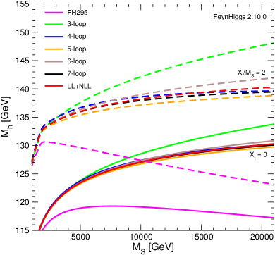
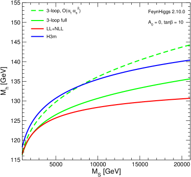
Figure 1: The mass of the lightest MSSM Higgs boson $M_{h}$ in dependence on the mass scale $M_{S}$.
Left: The “old” FeynHiggs result with no additional logarithmic contributions of 3- or higher loop order (pink), including analytically determined leading and next-to leading logarithmic contributions of 3- to 7-loop order (green, blue, yellow, brown, black) and including the numerically obtained resummed leading and next-to leading contributions (red) are shown for no mixing/maximal mixing (solid/dashed).
Right: The H3m result is shown in blue, the FeynHiggs result including leading and next-to leading logarithmic contributions of 3-loop order of $\mathcal{O}(\alpha_{t}\alpha_{s}^{2})$ and additionally of $\mathcal{O}(\alpha_{t}^{2}\alpha_{s})$ and $\mathcal{O}(\alpha_{t}^{3})$ is presented in green dashed and solid, respectively. The FeynHiggs result including the resummed logarithmic contributions is shown in red.
Parameters are chosen as described in the text.

On the right side of Fig. 1 a comparison of the FeynHiggs result with the known 3-loop order prediction of the Higgs mass is performed. The latter is obtained with the help of the program H3m [13]. In order to perform the comparison a CMSSM scenario has been chosen with the soft-breaking parameters $M_{0}=M_{1/2}=200\dots 15000$ GeV and $A_{0}=0$ and additionally $\tan\beta=10$ and $\mu>0$. The low-energy parameters have then been calculated with the spectrum generator SoftSUSY [24]. The following results are shown: the resummed leading and next-to leading log result (red), the result including only leading and next-to leading logarithmic terms up to 3-loop order (green, solid), the result including only up to leading and next-to leading logarithmic terms of order $\mathcal{O}(\alpha_{t}\alpha_{s}^{2})$ (green, dashed) and the result obtained with H3m (blue). The program H3m takes into account corrections up to order $\mathcal{O}(\alpha_{t}\alpha_{s}^{2})$. As it is calculated using the FD approach it includes all terms of this order, also non-logarithmic terms. Also, it takes into account different SUSY mass scales. Additionally, the applied renormalization schemes at two-loop order differ in H3m and FeynHiggs. With respect to these difference the $\mathcal{O}(\alpha_{t}\alpha_{s}^{2})$ results of both programs agree reasonably well. However, one can also see that the terms of $\mathcal{O}(\alpha_{t}^{2}\alpha_{s})$ and $\mathcal{O}(\alpha_{t}^{3})$ are important too and lead to a reduction of the size of the Higgs mass prediction.

6 Conclusion

The Higgs sector of the Minimal Supersymmetric Standard Model has been discussed. One important and easily measurable observable is the mass of the newly discovered particle which could be the lightest Higgs boson of the MSSM. To fully exploit this constraint, a precise prediction of the mass of the lightest Higgs boson is necessary. For lower SUSY mass scales the Feynman diagrammatic approach leads to a precise prediction taking into account all terms of a certain order, also non-logarithmic terms. For larger SUSY mass scales the renormalization group equation approach is advantageous as potentially large logarithms are resummed. The presented combination of both approaches improves the known Feynman diagrammatic results for larger SUSY mass scales. It is implemented into the program FeynHiggs and can be switched on by the user by setting the flag looplevel =3.

Further refinements, e.g. allowing for different mass scales or including higher-order contributions in the matching conditions, are planned.

References

- [1] G. Aad et al. [ATLAS Collaboration], Phys. Lett. B 716 (2012) 1, [arXiv:1207.7214 [hep-ex]].
- [2] S. Chatrchyan et al. [CMS Collaboration], Phys. Lett. B 716 (2012) 30, [arXiv:1207.7235 [hep-ex]].
-
[3]
M. Dugan, B. Grinstein and L. J. Hall,
Nucl. Phys. B 255 (1985) 413;
S. Dimopoulos and S. D. Thomas, Nucl. Phys. B 465 (1996) 23, [hep-ph/9510220]. - [4] G. Degrassi, S. Heinemeyer, W. Hollik, P. Slavich and G. Weiglein, Eur. Phys. J. C 28 (2003) 133, [hep-ph/0212020].
-
[5]
S. Heinemeyer, O. Stål and G. Weiglein,
Phys. Lett. B 710 (2012) 201
[arXiv:1112.3026 [hep-ph]];
A. Arbey, M. Battaglia, A. Djouadi, F. Mahmoudi and J. Quevillon, Phys. Lett. B 708 (2012) 612 [arXiv:1112.3028 [hep-ph]]. - [6] ATLAS Collaboration, ATLAS-CONF-2013-014.
- [7] CMS Collaboration, CMS-PAS-HIG-13-005
-
[8]
J. R. Ellis, G. Ridolfi and F. Zwirner,
Phys. Lett. B 257 (1991) 83;
A. Brignole, Phys. Lett. B 281 (1992) 284;
P. H. Chankowski, S. Pokorski and J. Rosiek, Phys. Lett. B 274 (1992) 191; Nucl. Phys. B 423 (1994) 437 [hep-ph/9303309];
A. Dabelstein, Z. Phys. C 67 (1995) 495 [hep-ph/9409375].
-
[9]
M. Frank T. Hahn, S. Heinemeyer, W. Hollik,
H. Rzehak and G. Weiglein,
JHEP 0702 (2007) 047,
[hep-ph/0611326].
- [10] S. Heinemeyer, W. Hollik and G. Weiglein, Eur. Phys. J. C 9 (1999) 343, [hep-ph/9812472].
-
[11]
R. Hempfling and A. H. Hoang,
Phys. Lett. B 331 (1994) 99,
[hep-ph/9401219];
G. Degrassi, P. Slavich and F. Zwirner, Nucl. Phys. B 611 (2001) 403, [hep-ph/0105096];
A. Brignole, G. Degrassi, P. Slavich and F. Zwirner, Nucl. Phys. B 631 (2002) 195, [hep-ph/0112177];
A. Brignole, G. Degrassi, P. Slavich and F. Zwirner, Nucl. Phys. B 643 (2002) 79, [hep-ph/0206101];
A. Dedes, G. Degrassi and P. Slavich, Nucl. Phys. B 672 (2003) 144, [hep-ph/0305127];
S. Heinemeyer, W. Hollik, H. Rzehak and G. Weiglein, Eur. Phys. J. C 39 (2005) 465, [hep-ph/0411114];
Phys. Lett. B 652 (2007) 300 [arXiv:0705.0746 [hep-ph]]. - [12] S. Martin, Phys. Rev. D 65 (2002) 116003, [hep-ph/0111209]; Phys. Rev. D 66 (2002) 096001, [hep-ph/0206136]; Phys. Rev. D 67 (2003) 095012, [hep-ph/0211366]; Phys. Rev. D 68 (2003) 075002, [hep-ph/0307101]; Phys. Rev. D 70 (2004) 016005 Phys. Rev. D 70 (2004) 016005, [hep-ph/0312092]; Phys. Rev. D 71 (2005) 016012, [hep-ph/0405022].
- [13] R. Harlander, P. Kant, L. Mihaila and M. Steinhauser, Phys. Rev. Lett. 100 (2008) 191602 [ibid. 101 (2008) 039901], [arXiv:0803.0672 [hep-ph]]; JHEP 1008 (2010) 104, [arXiv:1005.5709 [hep-ph]].
-
[14]
R. Barbieri, M. Frigeni and F. Caravaglios,
Phys. Lett. B 258 (1991) 167;
Y. Okada, M. Yamaguchi and T. Yanagida, Phys. Lett. B 262 (1991) 54; Prog. Theor. Phys. 85 (1991) 1. - [15] J. R. Espinosa and M. Quiros, Phys. Lett. B 266 (1991) 389;
- [16] H. E. Haber and R. Hempfling, Phys. Rev. D 48 (1993) 4280 [hep-ph/9307201].
-
[17]
J. A. Casas, J. R. Espinosa, M. Quiros and A. Riotto,
Nucl. Phys. B 436 (1995) 3
[Erratum-ibid. B 439 (1995) 466]
[hep-ph/9407389];
M. S. Carena, J. R. Espinosa, M. Quiros and C. E. M. Wagner, Phys. Lett. B 355 (1995) 209, [hep-ph/9504316];
Nucl. Phys. B 461 (1996) 407, [hep-ph/9508343]; R. -J. Zhang, Phys. Lett. B 447 (1999) 89, [hep-ph/9808299];
J. R. Espinosa and R. -J. Zhang, JHEP 0003 (2000) 026, [hep-ph/9912236];
J. R. Espinosa and I. Navarro, Nucl. Phys. B 615 (2001) 82, [hep-ph/0104047]. - [18] M. Carena, M. Quirós, C. E. M. Wagner, Nucl. Phys. B 461 (1996) 407, [hep-ph/9508343].
- [19] S. P. Martin, Phys. Rev. D 75 (2007) 055005 [hep-ph/0701051].
- [20] P. Draper, G. Lee and C. E. M. Wagner, Phys. Rev. D 89 (2014) 055023 [arXiv:1312.5743 [hep-ph]].
- [21] T. Hahn, S. Heinemeyer, W. Hollik, H. Rzehak and G. Weiglein, Phys. Rev. Lett. 112 (2014) 141801, [arXiv:1312.4937 [hep-ph]].
-
[22]
S. Heinemeyer, W. Hollik and G. Weiglein,
Comput. Phys. Commun. 124 (2000) 76,
[hep-ph/9812320];
T. Hahn, S. Heinemeyer, W. Hollik, H. Rzehak and G. Weiglein, Comput. Phys. Commun. 180 (2009) 1426, see www.feynhiggs.de. - [23] M. Carena, H. Haber, S. Heinemeyer, W. Hollik, C. Wagner and G. Weiglein, Nucl. Phys. B 580 (2000) 29, [hep-ph/0001002].
- [24] B. C. Allanach, Comput. Phys. Commun. 143 (2002) 305, [hep-ph/0104145].