Application of the phase space action principle to finite-size particle plasma simulations in the drift-kinetic approximation

Abstract

We formulate a finite-size particle numerical model of strongly magnetized plasmas in the drift-kinetic approximation. We use the phase space action as an alternative to previous variational formulations based on Low’s Lagrangian or on a Hamiltonian with a non-canonical Poisson bracket. The useful property of this variational principle is that it allows independent transformations of particle coordinates and velocities, i.e., transformations in particle phase space. With such transformations, a finite degree-of-freedom drift-kinetic action is obtained through time-averaging of the finite degree-of-freedom fully-kinetic action. Variation of the drift-kinetic Lagrangian density leads to a self-consistent, macro-particles and fields numerical model. Since the computational particles utilize only guiding center coordinates and velocities, there is a large computational advantage in the time integration part of the algorithm. Numerical comparison between the time-averaged fully-kinetic and drift-kinetic charge and current, deposited on a computational grid, offers insight into the range of validity of the model. Being based on a variational principle, the algorithm respects the energy conserving property of the underlying continuous system. The development in this paper serves to further emphasize the advantages of using variational approaches in plasma particle simulations.

1 Introduction

Finite-size particle algorithms for kinetic plasma simulations have established a strong record of success in a variety of areas[1, 2]. Recent work [3] reexamined the variational formulations of these algorithms [4, 5] and developed important improvements and generalizations. Two variational formulations were considered in Ref. [3], one based on Low’s Lagrangian [6], which generalized previous work and a new one, based on a Hamiltonian functional and a non-canonical Poisson bracket [7, 8]. Ref. [3] analyzed in detail the relation between Lagrangian symmetries and conservation properties in the process of reduction from infinite (Vlasov–Poisson or Vlasov–Maxwell system) to finite number of degrees of freedom (DOF), pointing out which approximations led to the retention – or not – of which conserved quantities. It also addressed the relation between force interpolation and particle shape and showed that the particle shape is not the determining factor in an algorithm’s overall accuracy; as an illustration, it constructed a charge deposition rule that has a narrow stencil but high smoothness. Energy conservation properties were carefully examined and was shown that in the time-discretized system, energy conservation depends only on the time step size; as a comparison, it showed that in the more standard particle-in-cell (PIC) algorithm energy conservation depends on both the time step and the grid spacing. There are many other attractive features of variational formulations, including the ease of change of variables, a consistent way of increasing the overall accuracy (in space and time), etc., which motivate us to seek their further extensions and applications.

The present work has two purposes. First, to offer an alternative formulation to the above two, a formulation based on the phase space action [9, 10]. In this variational principle the particle coordinates and velocities are considered independent variables and are varied separately. The physical relations between coordinates and velocities as well as Newton’s equations of motion are obtained after performing the variation. The important feature of this approach is that it allows transformation of variables independently for coordinates and velocities, i.e., transformations in particle phase space rather than in configuration space only. This property was used by Littlejohn [11], who offered a simplified derivation of the guiding center equations of motion of a point particle in external electric and strong magnetic fields. Thus, the second purpose of the present work is to introduce the guiding center equations of motion for finite size particles in a self-consistent, particles and fields numerical model. Since this is a variational formulation, the energy conserving property is automatically preserved.

We conduct a brief discussion of related literature to help point out certain novel aspects of our work. The early publication of Lee and Okuda [12] presented a particle model based on drift-kinetic electrons and fully-kinetic ions and used it to simulate the linear and non-linear stages of drift-wave instabilities. An important advantage of such approach was the large reduction in the computational cost due to the larger time step for pushing electrons; another advantage was the ability to use realistic electron-to-ion mass ratio. In a later publication, further computational efficiency was targeted by using gyro-kinetic ions in addition to the drift-kinetic electrons [13, 14]. These models were further developed in Refs. [15, 16] and were used to study magnetic reconnection [17]. The review article by Garbet et al. [18] provides a summary of other particle-based simulation efforts and available codes.

The main method followed by the above authors in obtaining a finite DOF system, i.e., a numerical model, was to first time- or gyro-phase average the fully-kinetic continuous equations to obtain drift- or gyro-kinetic continuous equations and then apply specific spatial and time descretizations. This is similar to the approach used in the PIC method. In doing so, existing conservation laws in the continuous system do not automatically transfer to the resulting numerical model. For example, the loss of energy conservation is due to errors of order higher than the discretization accuracy. It is known that nonphysical numerical artifacts occur in so-discretized systems [19, 20]. In contrast, our starting point is a finite DOF fully-kinetic system, i.e., a reduced Maxwell–Vlasov system described by finite-size particles and spatially discretized fields (with continuous time). To this reduced system, we then apply a time-averaging procedure to directly obtain a numerical model with finite-size particles and spatially discretized fields in the drift kinetic approximation (the gyro-kinetic approximation lies outside the scope of the present work). All steps, including those leading to the reduced fully-kinetic system and its time-averaging, are performed within the Lagrangian framework, which permits to preserve to the fullest the existing symmetries of the original continuous system; in particular, the energy-conserving property is preserved. Additional conservation laws may be respected depending on the specifics of the discretization [3]. In following this approach, we construct discretization schemes, in which discretization errors cancel out exactly to make the conservation of certain quantities possible. The Lagrangian framework is not mandatory in deriving such discretizations, however alternatively, one would be faced with the difficult task of tracking unbalanced errors and modifying discretizations to achieve the same effect.

The energy-conserving deficiency in the PIC model was addressed recently in two publications [21, 22]. In addition, a novel implicit technique was introduced that projects large computational advantage. Only fully-kinetic plasmas were addressed in these works.

Recent variational finite-size particle formulations were reported by several authors [23, 24, 25, 26]. These models were restricted to fully-kinetic electrostatic or electromagnetic plasmas. Another difference with the present work is that these authors use time and space discretized action vs. our use of continuous time and spatially discretized Lagrangian; in fact, our keeping time continuous is crucial in order to apply the time-averaging procedure to the fully-kinetic Lagrangian (A). The equations of our formulation are most suited to time-explicit schemes while those in the cited references result, as a rule, in time-implicit schemes [27] (e.g., when magnetic field is included or when higher than second order time integration is desired).

The rest of the paper is organized as follows. Section 2 describes an alternative formulation of finite-size particle algorithms based on the phase-space action. Section 3 describes the drift-kinetic approximation of the phase space action and the drift-kinetic numerical model. Section 4 provides numerical comparison between the fully-kinetic and the drift-kinetic models. Section 5 discusses the results and concludes.

2 Phase space variational principle

Our starting point is the phase space Lagrangian density (or simply Lagrangian) for the fully-kinetic system of particles and fields in Coulomb gauge [9, 10], reduced to a finite number of degrees of freedom [3]:

$$\mathcal{L}_{{}_{\rm FK}}= \,\sum_{\alpha=1}^{N_{\rm p}}\,w_{\alpha}\left[{{\tt m}}\mathbf{v}_{\alpha}+{{\tt q}}\mathbf{A}(\mathbf{x}_{\alpha},t)\right]\cdot\dot{\mathbf{x}}_{\alpha}$$

$$\!\!-\sum_{\alpha=1}^{N_{\rm p}}\,w_{\alpha}\left[\frac{1}{2}{{\tt m}}\mathbf{v}_{\alpha}^{2}+{{\tt q}}\varphi(\mathbf{x}_{\alpha},t)\right]$$

$$\!\!+h_{x}h_{y}h_{z}\left\{-\frac{\epsilon_{0}}{2}\!\sum_{\bf m,n}\,\varphi_{\bf m}(t)\nabla_{\bf mn}^{2}\varphi_{\bf n}(t)\right.$$

$$\left.\!\!+\,\frac{\epsilon_{0}}{2}\!\sum_{\bf m}\dot{\mathbf{A}}_{\mathbf{m}}(t)\cdot\dot{\mathbf{A}}_{\mathbf{m}}(t)+\!\frac{1}{2\mu_{0}}\!\sum_{\bf m,n}\!\mathbf{A}_{\bf m}(t)\cdot\nabla_{\bf mn}^{2}\mathbf{A}_{\bf n}(t)\right\}\!,$$ (1)

where $N_{\rm p}$ is the number of simulation particles; $w_{\alpha}$ is their computational weight; ${{\tt m}}$ and ${{\tt q}}$ are the physical mass and charge of the plasma species (we do not show explicitly a sum over particle species but such can be trivially added); $\epsilon_{0}$ and $\mu_{0}$ are the permittivity and permeability of vacuum; $\varphi_{\bf m}$ and $\mathbf{A}_{\bf m}$ denote the collection of grid (or nodal) values of the electric and magnetic vector potential, respectively, on a three-dimensional grid with $\mathbf{m}\equiv(m_{x},m_{y},m_{z})$; the grid is assumed uniform with grid spacings $h_{x}$, $h_{y}$, and $h_{z}$; sums in $\mathbf{m},\mathbf{n}$ range over all grid points; $\mathbf{x}_{\alpha}$ is the computational particle’s coordinate and $\dot{\mathbf{x}}_{\alpha}$ its time derivative; $\mathbf{v}_{\alpha}$ is the particle’s velocity, which at this point is considered an independent variable, i.e., unrelated to $\dot{\mathbf{x}}_{\alpha}$. The abbreviated notations $\varphi(\mathbf{x}_{\alpha},t)$ and $\mathbf{A}(\mathbf{x}_{\alpha},t)$ have been used to denote interpolated values of the electric and magnetic vector potential from the computational grid to the particle location:

$$\varphi(\mathbf{x}_{\alpha},t) =\,\sum_{\bf m}\,\rho_{\bf m}(\mathbf{x}_{\alpha})\varphi_{\bf m}(t)\,,$$ (2)

$$\mathbf{A}(\mathbf{x}_{\alpha},t) =\,\sum_{\bf m}\,\rho_{\bf m}(\mathbf{x}_{\alpha})\mathbf{A}_{\bf m}(t)\,.$$ (3)

$\rho_{\bf m}(\mathbf{x}_{\alpha})$ is a charge deposition rule of choice; $\rho_{\bf m}(\mathbf{x}_{\alpha})$ could either be chosen from some of the well known rules in the particle-in-cell method [1, 2] or from the more general ones described in [3]. The operator $\nabla^{2}_{\bf mn}$ denotes the appropriately discretized Laplacian operator, e.g., by central differences. Additionally, we introduce the following notation [which becomes apparent in deriving equations (6)–(9)]:

$${\bf B}(\mathbf{x}_{\alpha},t) =\nabla\times\mathbf{A}(\mathbf{x}_{\alpha},t)=\sum_{\bf m}\,\frac{\partial\rho_{\bf m}(\mathbf{x}_{\alpha})}{\partial\mathbf{x}_{\alpha}}\times\mathbf{A}_{\bf m}(t)\,,$$ (4)

$$\nabla\varphi(\mathbf{x}_{\alpha},t) =\sum_{\bf m}\,\frac{\partial\rho_{\bf m}(\mathbf{x}_{\alpha})}{\partial\mathbf{x}_{\alpha}}\,\varphi_{\bf m}(t)\,,\qquad$$

$$\frac{\partial A(\mathbf{x}_{\alpha},t)}{\partial t} =\sum_{\bf m}\,\rho_{\bf m}\left(\mathbf{x}_{\alpha}\right)\frac{{\rm d}\mathbf{A}_{\bf m}(t)}{{\rm d}t}\,,$$

$${\bf E}(\mathbf{x}_{\alpha},t) =-\nabla\varphi(\mathbf{x}_{\alpha},t)-\frac{\partial A(\mathbf{x}_{\alpha},t)}{\partial t}\,.$$ (5)

In the following part of the paper, where we do not show explicitly the arguments of field variables, we assume definitions similar to (2)–(5); we also assume the convention of summation over repeated indices.

The independent variables in the Lagrangian (1) are $(\mathbf{x}_{\alpha},\allowbreak\mathbf{v}_{\alpha},\varphi_{\bf m},\mathbf{A}_{\bf m})$. The equations for the electric and magnetic fields are obtained by a variation with respect to the corresponding variable, $\varphi_{\bf m}$ and $\mathbf{A}_{\bf m}$. Keeping in mind that independent variations of particle positions $\mathbf{x}_{\alpha}$ and velocities $\mathbf{v}_{\alpha}$ are performed in (1), we obtain

$$\dot{\mathbf{x}}_{\alpha} =\,\mathbf{v}_{\alpha}\,,$$ (6)

$${{\tt m}}\dot{\mathbf{v}}_{\alpha} =-{{\tt q}}\left[\nabla\varphi(\mathbf{x}_{\alpha},t)+\frac{\partial\mathbf{A}(\mathbf{x}_{\alpha},t)}{\partial t}\right]\!+{{\tt q}}\,\dot{\mathbf{x}}_{\alpha}\!\times\!\nabla\!\times\!\mathbf{A}(\mathbf{x}_{\alpha},t)\,$$

$$=\,\,{\tt q}\,\big{[}\mathbf{E}(\mathbf{x}_{\alpha},t)+\dot{\mathbf{x}}_{\alpha}\times\mathbf{B}(\mathbf{x}_{\alpha},t)\big{]}\,,$$ (7)

$$h_{x}h_{y}h_{z}\nabla_{\bf mn}^{2}\varphi_{\bf n}=-\frac{{\tt q}}{\epsilon_{0}}\sum_{\alpha=1}^{N_{\rm p}}\,w_{\alpha}\rho_{\bf m}(\mathbf{x}_{\alpha})\,,$$ (8)

$$h_{x}h_{y}h_{z}\frac{1}{\mu_{0}}\left[\nabla_{\bf mn}^{2}\mathbf{A}_{\bf n}-\frac{1}{c^{2}}\ddot{\mathbf{A}}_{\bf m}\right]=-{{\tt q}}\sum_{\alpha=1}^{N_{\rm p}}\,w_{\alpha}\dot{\mathbf{x}}_{\alpha}\rho_{\bf m}(\mathbf{x}_{\alpha})\,,$$ (9)

i.e., a self-consistent set of equations for macro-particles and (spatially discretized) fields. As already stated, the physical relation between coordinates $\mathbf{x}_{\alpha}$ and velocities $\mathbf{v}_{\alpha}$, Eq. (6), is obtained as a result of the variation.

We note that Eqs. (7)–(9) are suitable for the simulation of fully-kinetic electromagnetic plasmas, including electromagnetic waves, with the restriction that the particles have non-relativistic velocities; Ref. [28] offers a 1D relativistic formulation with Low’s Lagrangian as a starting point.

The energy is given by

$$W_{{}_{\rm FK}}= \frac{1}{2}\sum_{\alpha=1}^{N_{\rm p}}w_{\alpha}{\tt m}\dot{\mathbf{x}}_{\alpha}^{2}+\frac{\epsilon_{0}}{2}h_{x}h_{y}h_{z}\dot{\mathbf{A}}_{\bf m}\cdot\dot{\mathbf{A}}_{\bf m}$$

$$\mbox{}-h_{x}h_{y}h_{z}\left[\frac{\epsilon_{0}}{2}\varphi_{\bf m}\nabla_{\bf mn}^{2}\varphi_{\bf n}+\frac{1}{2\mu_{0}}\mathbf{A}_{\bf m}\nabla_{\bf mn}^{2}\mathbf{A}_{\bf n}\right].$$ (10)

The proof of the energy-conserving property is straightforward and is herein omitted.

3 The drift-kinetic approximation

The more general transformation of variables in the phase space action principle was exploited by Littlejohn [11] to great advantage. He presented a mathematically simple and elegant derivation of the guiding center equations of motion of a point particle in external electric and strong magnetic fields. The derivations in Littlejohn’s paper may be repeated with minor modifications to account for the finite size of computational particles. We remind the reader that the guiding center approximation aims to filter out the fast gyro-motion and describe the particle motion by an “averaged,” guiding center motion. An important assumption is the smallness of the gyro-radius of a particle compared to the length scale of interest. Thus, in deriving the guiding center Lagrangian, certain ordering between the various quantities is assumed. For example, in Littlejohn’s derivation the $\mathbf{E}\times\mathbf{B}$ velocity drift is assumed to be of the same order as the $\nabla B$ and curvature $B$ drifts. This imposes a limitation on the magnitude of the electric field. One may also consider the case of a strong $\mathbf{E}\times\mathbf{B}$ shear (see Ref. [29] and references therein); then the details of the averaging procedure must reflect such choice. In the present work we adhere to Littlejohn’s choice of ordering. Last, we assume that the perturbation fields, i.e., fields due to plasma space charge and plasma currents, are weak so that do not violate the drift-kinetic ordering. We do not consider directions parallel and perpendicular to the magnetic field separately since we retain the possibility to treat one of the plasma species as fully-kinetic, i.e., not strongly magnetized. Ultimately, the validity of a drift-kinetic model lies within the made assumptions.

We obtain (see A and Ref. [11]) the Lagrangian of particles and fields corresponding to the lowest, drift-kinetic ordering in the small parameter as:

$$\mathcal{L}_{\!{}_{\rm DK}}= \,\sum_{\alpha=1}^{N_{\rm p}}w_{\alpha}\!\left[{{\tt q}}\mathbf{A}+{{\tt m}}U_{\alpha}\hat{\mathbf{b}}\right]\cdot\dot{\mathbf{X}}_{\alpha}+\left(\frac{{\tt m}}{{\tt q}}\right)\sum_{\alpha=1}^{N_{\rm p}}\,w_{\alpha}\mu_{\alpha}\dot{\Psi}_{\alpha}$$

$$-\sum_{\alpha=1}^{N_{\rm p}}w_{\alpha}\!\left[{{\tt q}}\varphi+\mu_{\alpha}B+\frac{{\tt m}U_{\alpha}^{2}}{2}\right]$$

$$+h_{x}h_{y}h_{z}\left\{-\frac{\epsilon_{0}}{2}\varphi_{\bf m}(t)\nabla_{\bf mn}^{2}\varphi_{\bf n}(t)\right.$$

$$\left.+\frac{\epsilon_{0}}{2}\dot{\mathbf{A}}_{\mathbf{m}}(t)\cdot\dot{\mathbf{A}}_{\mathbf{m}}(t)+\!\frac{1}{2\mu_{0}}\mathbf{A}_{\bf m}(t)\cdot\nabla_{\bf mn}^{2}\mathbf{A}_{\bf n}(t)\right\}\,.$$ (11)

The definitions of the various quantities in (11) are as follows: $\mathbf{X}_{\alpha}$ is the guiding center coordinate of particle $\alpha$ and $\dot{\mathbf{X}}_{\alpha}$ its time derivative; $U_{\alpha}$ is the particle’s velocity parallel to the magnetic field line (again, in (11) it is considered unrelated to $\dot{\mathbf{X}}_{\alpha}$); $\Psi_{\alpha}$ is the gyro-phase of the particle; $B=\sqrt{(\nabla\times\mathbf{A}(\mathbf{X}_{\alpha},t))^{2}}$ is the magnitude of the magnetic field; $\hat{\mathbf{b}}(\mathbf{X}_{\alpha},t)=\mathbf{B}(\mathbf{X}_{\alpha},t)/B(\mathbf{X}_{\alpha},t)$ is the unit vector in the direction of the magnetic field; $\mu_{\alpha}={{\tt m}}v_{\alpha_{\perp}}^{2}/(2B)$ is the magnetic moment of the particle with velocity $v_{\alpha_{\perp}}$ perpendicular to the magnetic field line (see also A).

The independent variables in the Lagrangian (11) are$(\mathbf{X}_{\alpha},U_{\alpha},\mu_{\alpha},\Psi_{\alpha},\varphi_{\bf m},\mathbf{A}_{\bf m})$. One can easily see that a variation with respect to $\mu_{\alpha}$ yields the decoupled equation $\dot{\Psi}_{\alpha}=({{\tt q}}/{{\tt m}})B$, a variation with respect to the gyro-phase yields the conservation of the particle’s magnetic moment, $\dot{\mu}_{\alpha}=0$, and a variation with respect to $U_{\alpha}$ yields $U_{\alpha}=\hat{\mathbf{b}}\cdot\dot{\mathbf{X}}_{\alpha}$. The remaining variations of the Lagrangian (11) with respect to ${\mathbf{X}}_{\alpha}$, $\varphi_{\bf m}$, and $\mathbf{A}_{\bf m}$ yield the self-consistent set of equations:

$$\dot{\mathbf{X}}_{\alpha}= \,\frac{1}{\hat{\mathbf{b}}\cdot\mathbf{B}^{*}}\left\{U_{\alpha}\mathbf{B}^{*}+\hat{\mathbf{b}}\times\big{[}(\mu_{\alpha}/{\tt q})\nabla B-\mathbf{E}^{*}\big{]}\right\}\,,$$ (12)

$${{\tt m}}\dot{U}_{\alpha}= -\frac{{\tt q}}{\hat{\mathbf{b}}\cdot\mathbf{B}^{*}}\mathbf{B}^{*}\cdot\big{[}(\mu_{\alpha}/{\tt q})\nabla B-\mathbf{E}^{*}\big{]}\,,$$ (13)

$$h_{x}h_{y}h_{z}\,\epsilon_{0}\nabla_{\bf mn}^{2}\varphi_{\bf n}=-{\tt q}\sum_{\alpha=1}^{N_{\rm p}}\,w_{\alpha}\rho_{\bf m}(\mathbf{X}_{\alpha})\,,$$ (14)

$$h_{x}h_{y}h_{z}\,\frac{1}{\mu_{0}}\left(\nabla_{\bf mn}^{2}\mathbf{A}_{\rm n}-(1/c^{2})\ddot{\mathbf{A}}_{\bf m}\right)=$$

$$\mbox{\hskip 20.0pt}-{{\tt q}}\sum_{\alpha=1}^{N_{\rm p}}\,w_{\alpha}\dot{\mathbf{X}}_{\alpha}\rho_{\bf m}(\mathbf{X}_{\alpha})$$

$$\mbox{\hskip 20.0pt}+\sum_{\alpha=1}^{N_{\rm p}}\,w_{\alpha}\nabla\rho_{\bf m}(\mathbf{X}_{\alpha})\times\frac{{{\tt m}}\left(\dot{\mathbf{X}}_{\alpha}\dot{\mathbf{X}}_{\alpha}-U_{\alpha}^{2}\mathbf{I}\right)\cdot\hat{\mathbf{b}}(\mathbf{X}_{\alpha})}{B(\mathbf{X}_{\alpha})}$$

$$\mbox{\hskip 20.0pt}-\sum_{\alpha=1}^{N_{\rm p}}\,w_{\alpha}\mu_{\alpha}\nabla\rho_{\bf m}(\mathbf{X}_{\alpha})\times\hat{\mathbf{b}}(\mathbf{X}_{\alpha})\,$$ (15)

with unity tensor ${\bf I}$ and

$$\mathbf{B}^{*}=\mathbf{B}+{{\tt m}}U_{\alpha}\nabla\times\hat{\mathbf{b}},\quad\mathbf{E}^{*}=\mathbf{E}-({{\tt m}/{\tt q}})U_{\alpha}\frac{\partial\hat{\mathbf{b}}}{\partial t}\,.$$ (16)

Eqs. (12) and (13) are the well known guiding center equations of motion. Eqs. (14) and Eq. (15), Poisson’s and the wave equation, include self-consistently the plasma response. Notice that these equations contain only the guiding center particle coordinates and velocities. Therefore, the resulting electric and magnetic fields correspond to the time-averaged electric and magnetic fields of the full-kinetic model, Eqs. (6)–(9) (See also Sec. 4). This means that physics phenomena developing on the faster, gyro-motion time scale (e.g., for drift-kinetic electrons, the electron cyclotron resonance wave–particle interaction) are not included in this model.

The inclusion of electromagnetic waves, i.e., the wave equation (15), is only necessary when the physics requires it; for example, with drift-kinetic electrons and fully-kinetic ions, ion cyclotron resonance heating may be studied. Such numerical model may be constructed by adding the particle and interaction parts of the fully-kinetic Lagrangian (1) to the drift-kinetic Lagrangian (11). When wave–particle resonance physics in not of interest, the appropriate model is electrostatic and magnetostatic. Such model may be obtained by setting $\dot{\mathbf{A}}_{\mathbf{m}}(t)=0$ in the Lagrangian (11); then the term $(1/c^{2})\ddot{\mathbf{A}}_{\bf m}$ in equation (15) is missing and each of the three components of the vector potential satisfies a Poisson equation.

Defining $\mathbf{M}_{\alpha}={{\tt m}}\dot{\mathbf{X}}_{\alpha}\dot{\mathbf{X}}_{\alpha}/B$ and a projection operator $\mathbf{\Pi}_{\perp}={\bf I}-\hat{\mathbf{b}}\hat{\mathbf{b}}$, the second term on the right-hand-side of (15) can be written as $\sum_{\alpha}^{N_{\rm p}}w_{\alpha}\nabla\rho_{\bf m}(\mathbf{X}_{\alpha})\times\mathbf{\Pi}_{\perp}\cdot\mathbf{M}_{\alpha}\cdot\hat{\mathbf{b}}$; thus we note two magnetic moment contributions to the current, Eq. (15): one from the intrinsic gyro-motion, $\mu_{\alpha}$, and one from the drifting guiding center motion, $\mathbf{M}_{\alpha}$.

The energy of the drift-kinetic model is given by

$$W_{{}_{\rm DK}}= \sum_{\alpha=1}^{N_{\rm p}}w_{\alpha}\left[\frac{{\tt m}}{2}U_{\alpha}^{2}+\mu_{\alpha}B\right]+\frac{\epsilon_{0}}{2}h_{x}h_{y}h_{z}\dot{\mathbf{A}}_{\bf m}\cdot\dot{\mathbf{A}}_{\bf m}$$

$$-h_{x}h_{y}h_{z}\left[\frac{\epsilon_{0}}{2}\varphi_{\bf m}\nabla_{\bf mn}^{2}\varphi_{\bf n}+\frac{1}{2\mu_{0}}\mathbf{A}_{\bf m}\nabla_{\bf mn}^{2}\mathbf{A}_{\bf n}\right].$$ (17)

The energy-conserving property is proved in B.

4 Comparison between the full and drift-kinetic models

In this section we study the applicability range of the self-consistent drift-kinetic numerical model.

In view of the extensive previous work on the guiding center equations of motion [30, 31, 32], we do not further test their validity. Instead, we focus on verifying that the time-averaged charge and current grid densities in the fully-kinetic equations, i.e., the time-averaged right-hand sides of Eqs. (8) and (9), correspond to their drift-kinetic counterparts, the right-hand sides of Eqs. (14) and (15).

Without having to implement a full three-dimensional particle code, here we present a more limited yet insightful numerical evidence. Namely, we consider the case of particles gyrating in a uniform magnetic and zero electric fields. This means that we exclude velocity drifts from consideration, i.e., we set $\dot{\mathbf{X}}_{\alpha}=0$. The assumption of zero parallel velocity does not present a restriction in a uniform magnetic field since the parallel component of the fully-kinetic velocity equals the parallel component of the guiding center velocity; the parallel current comparison then reduces to comparison of the charge deposition, as seen from the right-hand side of Eq. (9) and the first term on the right-hand side of Eq. (15). Last, we perform only single particle comparisons; again, this is not a restriction since the charge and current are additive in the number of particles (of course, keeping in mind that errors are also additive). To summarize, we compare the time-averaged fully-kinetic and drift-kinetic charge and current grid depositions for a single particle in a uniform magnetic and zero electric fields.

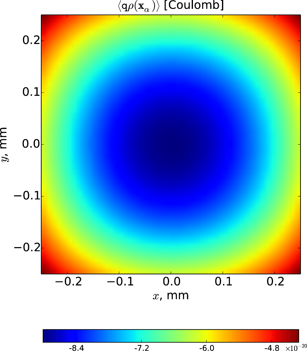
(a) Charge deposition by a test electron macro-particle placed at different locations within the cell. Largest negative charge is deposited at the center of the cell.

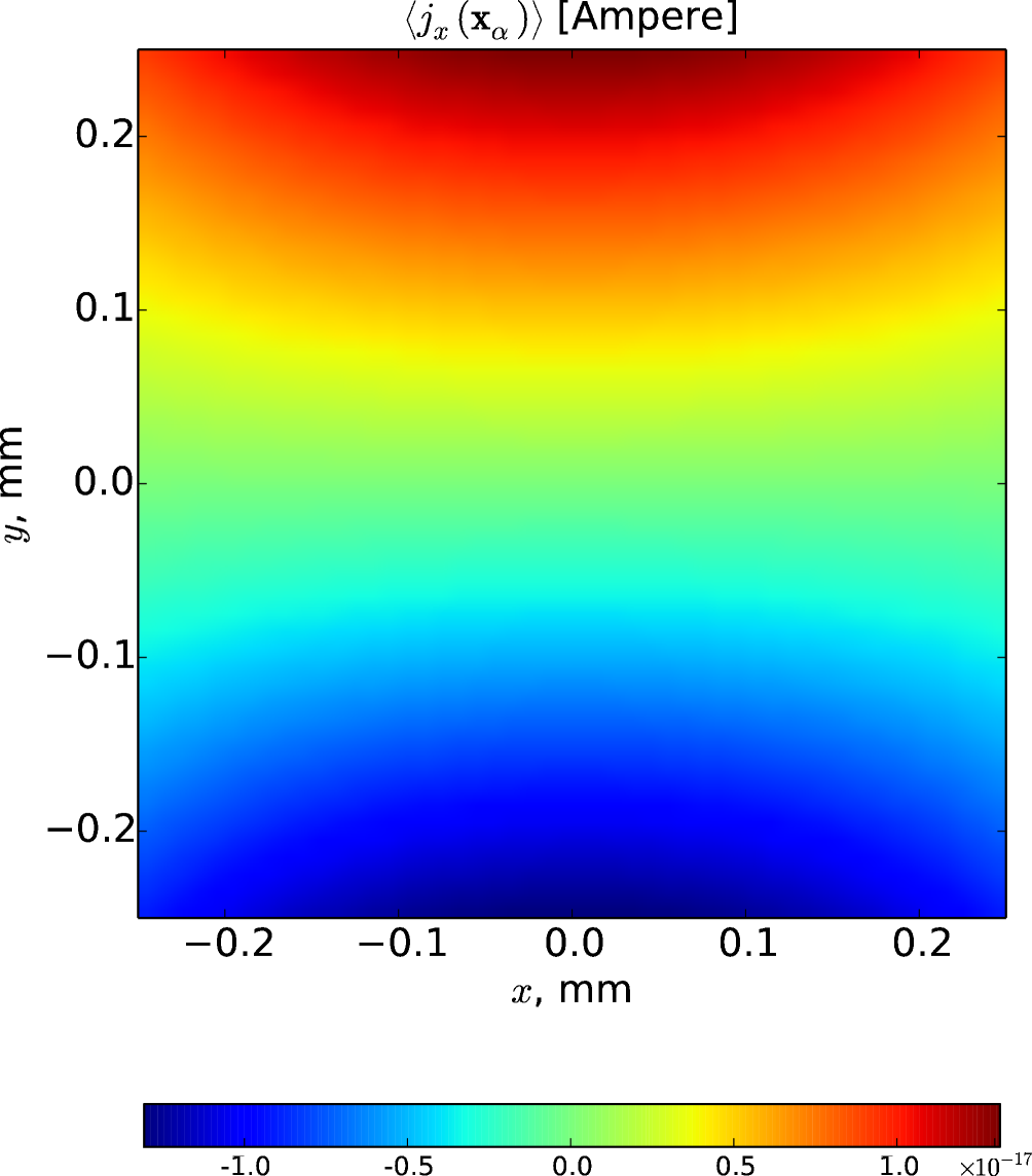
(b) Current deposition $\left<j_{x}(\mathbf{x}_{\alpha})\right>$ by a test electron macro-particle placed at different locations within the cell. Largest values (positive in the upper half) of the $x$-component of the current are at the top and bottom (horizontal) edges of the cell.

Figure 1: Grid deposition of charge and current.

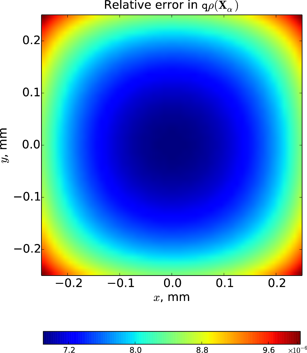
(a) Relative error in the charge deposition by a test electron macro-particle placed at different locations within the cell. Largest error is at the corners of the cell.

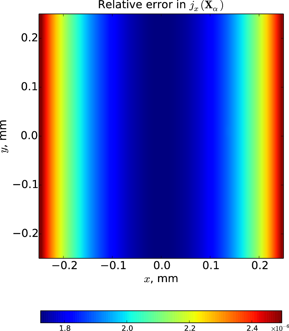
(b) Relative error in the current deposition by a test electron macro-particle placed at different locations within the cell. Largest error is along the vertical edges of the cell.

Figure 2: Relative error in the grid deposition of charge and current.

Let us define the time-average of a quantity $f(\mathbf{x}_{\alpha},t)$ as:

$$\left<f(\mathbf{x}_{\alpha})\right>=\frac{1}{T}\int_{0}^{T}\!{\rm d}\tau\,f(\mathbf{x}_{\alpha},\tau),$$ (18)

where $T$ is the particle’s gyro-period. We note that after averaging over the gyro-period, the quantity $f$ retains time dependence on the longer, drift-kinetic time scale (time argument not shown in (18)). We define the relative error of a grid quantity $f$ as

$$\mbox{Relative error}=\mbox{abs}\left(\frac{\left<f(\mathbf{x}_{\alpha})\right>-f(\mathbf{X}_{\alpha})}{\left<f(\mathbf{x}_{\alpha})\right>}\right)\,.$$ (19)

This is a measure of how well a drift-kinetic quantity approximates the time-averaged fully-kinetic quantity on the computational grid. With these definitions, we numerically verify the following equalities:

$$\left<{\tt q}\,\rho(\mathbf{x}_{\alpha})\right>= \,{\tt q}\,\rho(\mathbf{X}_{\alpha}),$$ (20)

$$\left<j_{x}(\mathbf{x}_{\alpha})\right>\equiv \,\left<{\tt q}\,\dot{x}_{\alpha}\rho(\mathbf{x}_{\alpha})\right>=\mu_{\alpha}\frac{\partial\rho(\mathbf{X}_{\alpha})}{\partial Y_{\alpha}}\equiv j_{x}(\mathbf{X}_{\alpha})\,,$$ (21)

$$\left<j_{y}(\mathbf{x}_{\alpha})\right>\equiv \,\left<{\tt q}\,\dot{y}_{\alpha}\rho(\mathbf{x}_{\alpha})\right>=-\mu_{\alpha}\frac{\partial\rho(\mathbf{X}_{\alpha})}{\partial X_{\alpha}}\equiv j_{y}(\mathbf{X}_{\alpha})\,,$$ (22)

where in the last two equations we have expanded the cross product in the third term on the right-hand side of Eq. (15), the only non-zero term in our case. We note that the current deposition (21) and (22) is independent of the sign of the charge; this is because reversing the sign of the charge reverses the direction of gyration of the particle, leaving the time-average unchanged ($\mu_{\alpha}>0$ by definition). In the general case $\dot{\mathbf{X}}_{\alpha}\neq 0$ the dependence of the drift-kinetic current on the sign of $q$ shows in the first term on the right-hand-side of (15); however, notice that the second term in that equation is also independent of the sign of ${\tt q}$.

For all numerical tests, we choose $h_{x}=h_{y}$ and use a single electron macro-particle (negative charge and computational weight $w_{\alpha}=1$). The magnetic field is oriented in the positive $z$-direction. The charge deposition rule (interpolating function) is chosen to be a quadratic spline; however, in a full implementation one would desire an interpolating function with two continuous derivatives (second derivative with respect to the particle coordinate $\mathbf{X}_{\alpha}$ appears in the term $\nabla B$), such a cubic spline, to ensure continuity of the force as a particle moves across cell boundaries.

In figure 1 we presents a view of the time averages of the fully-kinetic charge and current deposited on the nearest grid point; that is, the amount deposited on that grid point as a function of the particle location. The particle locations were chosen uniformly within the cell with $|x_{\alpha}|<h_{x}/2$ and $|y_{\alpha}|<h_{y}/2$. The electron macro-particle was initialized with the same velocity at each location, $v_{\perp}=10^{5}\,$m/s ($v_{x}=-v_{\perp}/\sqrt{2}$, $v_{y}=v_{\perp}/\sqrt{2}$), in a magnetic field of $0.5\,$T. Although the amount of deposited charge and current on one grid point changes, the total charge and current, which are found by summing the contributions from all grid points, are conserved. The time average of the charge deposition is symmetric about the cell center, as expected. The time average of the current, $\left<j_{x}\right>$ (Fig. 1(b)), is antisymmetric about $y=0$ since the particle contributes the exact same current in the positive and negative $y$-directions. Similarly, the current deposition $\left<j_{y}\right>$ is antisymmetric about $x=0$ (not shown).

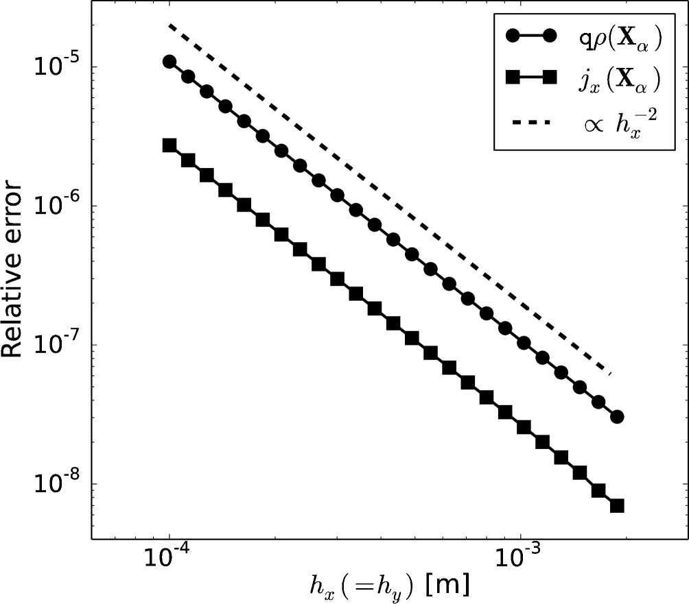
(a) Relative error in the charge and current deposition as a function of grid spacing.

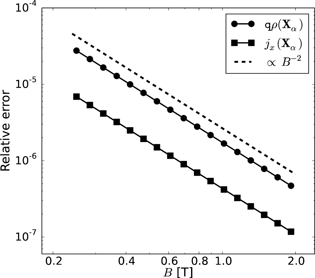
(b) Relative error in the charge and current deposition as a function of magnetic field strength.

Figure 3: Scaling of relative error.

Figure 2 shows the relative error in the deposited charge and current from figure  1, as defined in (19). The error in the deposited charge (Fig. 2(a)) is largest around the corners of the cell and is minimal at the center. The error in the deposited current (Fig. 2(b)) peaks at the left and right edges of the cell and is symmetric around $x=0$. Such variations of the error are related to the particular choice of interpolating function.

Next, figure 3 shows the variation of the relative errors with grid spacing and magnetic field strength. We have fixed the particle location near the center of the cell. For the dependence on the grid spacing shown in figure 3(a) we have set $B_{0}=2\,$T and $v_{\perp}=10^{5}\,$m/s. For the dependence on the magnetic field strength, figure 3(b), we have chosen $h_{x}=0.5\,$mm. The relative error in both the charge and current depositions decreases inversely with increasing grid spacing, $h_{x}$, and magnetic field strength, $B$. This is expected since finite Larmor radius effects become less important for larger $h_{x}$, i.e., the gyration of the particle becomes more “invisible” to the grid. Increasing the magnetic field strength achieves a similar effect since the gyro-radius decreases inversely with $B$. Recall that the validity of the drift-kinetic approximation depends on a small parameter, the ratio of the Larmor radius to the length scale of interest. In our case, the length scale of interest is given by the grid spacing, $h_{x}$. Either larger grid spacing or smaller gyro-radius decreases the value of this small parameter, improving the validity of the drift-kinetic approximation; this is reflected in the decreasing errors in figure 3. The particular scaling law of the relative error depends on the choice of interpolation rule. In our case, we see an inverse square dependence in both Figs. 3(a) and 3(b).

5 Discussion and conclusions

Using the phase space action principle, we have formulated an energy conserving (continuous time), finite-size particle, self-consistent numerical simulation model in the drift kinetic approximation. This work extends previous variational formulations. The model can be applied to simulate plasmas in strong magnetic fields where the electron (and possibly the ion) population of a plasma is highly magnetized and where kinetic effects are of importance. For example, in magnetized plasma discharges the electrons have a very non-Maxwellian velocity distribution. For such plasmas, fluid descriptions are inappropriate. Withing this category falls the modeling of electron cyclotron resonance ion sources (ECRIS) [33], where the electron population is strongly non-Maxwellian. Partial simulation results with the quasi-3D code SIMPL (SIMulation of PLasmas) [34] are in excellent agreement with the tests presented here. SIMPL utilizes the hybrid model of drift-kinetic electrons and fully-kinetic ions briefly described in Sec. 3.

Errors in the charge and current deposition on the computational grid were examined. It was shown that increasing the grid spacing and the magnetic field leads to decreasing of the error. This is an indication that the drift-kinetic approximation becomes better; it also serves as a guideline for the model applicability.

We note a certain limitation of the drift-kinetic Lagrangian (11). It was shown in Ref. [35] that at very large particle velocities and for magnetic fields with non-vanishing parallel curl, singularities in the guiding-center velocity and acceleration appear. The velocities at which this happens are usually very large, possibly larger than the speed of light for non-relativistic models; therefore, most applications may be unaffected by this divergence. In the cases when this singularity does occur, an appropriate regularization procedure of the drift-kinetic Lagrangian is available [35] and can be adapted to our numerical model.

The computational advantage of the method comes from the ability to increase the simulation time step by roughly two orders of magnitude; this is because the guiding center equations of motion are used, making it unnecessary to resolve the fast time scale of gyro-motion. In this model, physics developing on the gyro-period time scale is excluded.

We note that continuity of the force on a particle, as it crosses cell boundaries, is desirable but not mandatory. The energy conserving property of models with discontinuous particle force is still preserved [4, 5]; in fact, the energy variation in time is bounded when symplectic time integrators are used. The disadvantage is that the error scales more poorly with the time step (in the time-discretized model) compared to models using smoother interpolating functions [3, 36]. Numerical noise in simulations with discontinuous force is also higher. (To draw a parallel with the particle-in-cell method, the nearest-grid point charge deposition also has a discontinuous force and results in higher numerical noise.) Ref. [3] was able to considerably improve the numerical noise and the accuracy of energy conservation by providing the freedom to use smooth interpolating functions of any order. In the present formulation, the cubic spline is the lowest order interpolating function that possesses two continuous derivatives of $\rho_{\bf m}(\mathbf{X}_{\alpha})$. It is, of course, possible to use interpolating functions of order higher than cubic; however, a potential disadvantage is the higher computational load, which would diminish to an extent the advantage gained by using larger time steps. We postpone a more thorough examination of the trade-offs between the advantages and disadvantages of our model for the future, when a full implementation is available.

It is possible to generalize the method to higher order in the small (drift-kinetic ordering) parameter; however this would also require higher computational load and may become disadvantageous. Another possible generalization is constructing hybrid fluid–kinetic or fluid–drift-kinetic energy-conserving numerical models for magnetized plasmas; examples of such formulations for electrostatic plasmas are given in Refs.[3, 37].

The presented work underlines the advantages of using variational approaches to formulations of finite-size particle algorithms.

Appendix A Modification of the Lagrangian averaging procedure for finite size particles

In this appendix we outline the differences that arise when deriving the guiding center Lagrangian for finite-size (computational) particles. In the point particles case, the averaging procedure is effected through changes of variables and “gauge” transformations [11]. The procedure is based on particular ordering assumptions, small ratio of gyro-radius to length scale of interest and slow time variation of the magnetic vector potential and the electric potential. The following coordinate and velocity transformations are performed in the kinetic Lagrangian (1):

$$\mathbf{x}_{\alpha} =\mathbf{X}_{\alpha}+v_{\alpha_{\perp}}\hat{\mathbf{a}}(\mathbf{X}_{\alpha},t)/B(\mathbf{X}_{\alpha},t)\,,$$ (23)

$$\mathbf{v}_{\alpha} =U_{\alpha}\hat{\mathbf{b}}(\mathbf{X}_{\alpha},t)+v_{\alpha_{\perp}}\hat{\mathbf{c}}(\mathbf{X}_{\alpha},t)\,,$$ (24)

where the various unit vectors have the relation $\hat{\mathbf{a}}=\hat{\mathbf{b}}\times\hat{\mathbf{c}}$. In (23) and (24) the guiding center variables, $\mathbf{X}_{\alpha}$ and $U_{\alpha}$, are functions of the slow time; so is the magnitude of the perpendicular velocity, $v_{\alpha_{\perp}}$. To cancel out fast time scale terms, one makes transformations of the Lagrangian by adding the full time derivative of particular, carefully chosen functions; such addition does not change the equations of motion.

In our case this procedure needs to be performed on the finite-size particles Lagrangian, Eq. (1). Since time in (1) is continuous, i.e., only spatial discretization has been performed, adding a full time derivative of any function of particle and (discrete) fields does not change the equations of motion. For example, one of the transformations [11] uses the function:

$$S=-\left[\frac{\hat{\mathbf{a}}\,v_{\alpha_{\perp}}}{B}\right]\cdot\mathbf{A}\,.$$ (25)

The analogous function in terms of the variables in (1) becomes:

$$S=-\left[\frac{v_{\alpha_{\perp}}}{B(\mathbf{X}_{\alpha},t)}\right]\hat{\mathbf{a}}(\mathbf{X}_{\alpha},t)\cdot\mathbf{A}_{\bf m}(t)\rho_{\bf m}(\mathbf{X}_{\alpha})\,.$$ (26)

The full time derivative of (26) is evaluated as:

$$\frac{{\rm d}S}{{\rm d}t}= \,-\left[\frac{\hat{\mathbf{a}}\,v_{\alpha_{\perp}}}{B}\right]\cdot\mathbf{A}_{\bf m}\rho_{\bf m}(\mathbf{X}_{\alpha})\,\left[\dot{\mathbf{X}}_{\alpha}\cdot\nabla\rho_{\bf m}(\mathbf{X}_{\alpha})\right]$$

$$-\left[\frac{\hat{\mathbf{a}}\,v_{\alpha_{\perp}}}{B}\right]\cdot\dot{\mathbf{A}}_{\bf m}(t)\rho_{\bf m}(\mathbf{X}_{\alpha})$$

$$-\frac{{\rm d}}{{\rm d}t}\left[\frac{\hat{\mathbf{a}}\,v_{\alpha_{\perp}}}{B}\right]\cdot\mathbf{A}_{\bf m}(t)\,\rho_{\bf m}(\mathbf{X}_{\alpha})\,.$$ (27)

Expression (27) in conjunction with the assumed ordering of time scales is then used to obtain the averaged drift kinetic Lagrangian (11); we refer the reader to Ref. [11] for details.

Appendix B Proof of the energy conserving property of the drift-kinetic model

In this appendix we prove explicitly that the drift-kinetic approximation model, Eqs. (12)–(15), conserves energy when time is kept continuous. In a time-discretized model energy will not be strictly conserved; however, symplectic time integrators make its variation bounded and decreasing with smaller time step.

The following is a useful auxiliary identity, obtained by crossing Eq. (12) with $\mathbf{B}^{*}$, rearranging, and dotting with $\dot{\mathbf{X}}_{\alpha}$:

$$\frac{U_{\alpha}}{\mathbf{\hat{b}}\cdot\mathbf{B}^{*}}\mathbf{B}^{*}\cdot\left[\frac{\mu_{\alpha}}{{\tt q}}\nabla B-\mathbf{E}^{*}\right]= \,\frac{\mu_{\alpha}}{{\tt q}}\dot{\mathbf{X}}_{\alpha}\cdot\nabla B-\dot{\mathbf{X}}_{\alpha}\cdot\mathbf{E}^{*}.$$ (28)

The next two useful identities follow from definition (4):

$$\dot{\mathbf{A}}_{\bf m}\cdot\nabla\rho_{\bf m}\times\dot{\mathbf{X}}_{\alpha}= -\dot{\mathbf{X}}_{\alpha}\cdot\frac{\partial\mathbf{B}}{\partial t}\,,$$ (29)

$$\dot{\mathbf{A}}_{\bf m}\cdot\nabla\rho_{\bf m}\times{\hat{\mathbf{b}}}= -\hat{\mathbf{b}}\cdot\frac{\partial\mathbf{B}}{\partial t}\equiv-\frac{\partial{B}}{\partial t}\,.$$ (30)

The time derivative of the energy (17) is

$$\frac{{\rm d}W_{{}_{\rm DK}}}{{\rm d}t}= \,\sum_{\alpha}w_{\alpha}\left[{\tt m}U_{\alpha}\dot{U}_{\alpha}+\mu_{\alpha}\frac{{\rm d}B}{{\rm d}t}\right]$$

$$-h_{x}h_{y}h_{z}\epsilon_{0}\varphi_{\bf m}\nabla_{\bf mn}^{2}\dot{\varphi}_{\bf n}$$

$$+h_{x}h_{y}h_{z}\frac{1}{\mu_{0}}\dot{\mathbf{A}}_{\bf m}\cdot\left[\frac{1}{c^{2}}\ddot{\mathbf{A}}_{\bf m}-\nabla_{\bf mn}^{2}\mathbf{A}_{\bf n}\right]\,.$$ (31)

In Eq. (31), we use Eq. (13) with Eq. (28), expand the full time derivative of $B$ and use the definition of $\mathbf{E}^{*}$ from Eq. (16), use Eq. (15) and the time derivative of Eq. (14) to obtain

$$\frac{{\rm d}W_{{}_{\rm DK}}}{{\rm d}t}= \sum_{\alpha}w_{\alpha}\left[-\mu_{\alpha}\mathbf{X}_{\alpha}\cdot\nabla B+{\tt q}\mathbf{X}_{\alpha}\cdot\left(\mathbf{E}-\frac{{\tt m}}{{\tt q}}U_{\alpha}\frac{\partial\hat{\mathbf{b}}}{\partial t}\right)\right.$$

$$\mbox{\hskip 48.0pt}\left.+\mu_{\alpha}\frac{\partial B}{\partial t}+\mu_{\alpha}\mathbf{X}_{\alpha}\cdot\nabla B\right]$$

$$\mbox{}+\sum_{\alpha}w_{\alpha}{\tt q}\dot{\mathbf{X}}_{\alpha}\cdot\left[\varphi_{\bf m}\frac{\partial{\rho_{\bf m}}}{\partial\mathbf{X}_{\alpha}}+\rho_{\bf m}\dot{\mathbf{A}}_{\bf m}\right]$$

$$\mbox{}+\sum_{\alpha}w_{\alpha}\frac{{\tt m}U_{\alpha}}{B}\left(\dot{\mathbf{X}}_{\alpha}\cdot\frac{\partial\mathbf{B}}{\partial t}-U_{\alpha}\frac{\partial B}{\partial t}\right)$$

$$\mbox{}-\sum_{\alpha}w_{\alpha}\mu_{\alpha}\frac{\partial B}{\partial t}$$

$$= \sum_{\alpha}w_{\alpha}{\tt m}U_{\alpha}\!\left[\frac{1}{B}\left(\dot{\mathbf{X}}_{\alpha}\cdot\frac{\partial\mathbf{B}}{\partial t}-U_{\alpha}\frac{\partial B}{\partial t}\right)-\dot{\mathbf{X}}_{\alpha}\cdot\frac{\partial\hat{\mathbf{b}}}{\partial t}\right]$$

$$= \,\,0\,$$ (32)

after a number of obvious cancellations, using definition (5), and the last equality following from expanding

$$\frac{\partial\hat{\mathbf{b}}}{\partial t}\equiv\frac{\partial}{\partial t}\left(\frac{\mathbf{B}}{B}\right)=\frac{1}{B}\left(\frac{\partial\mathbf{B}}{\partial t}-\frac{\partial B}{\partial t}\hat{\mathbf{b}}\right)\,.$$

References

- Birdsall and Langdon [1991] \bibinfoauthorC. K. Birdsall, \bibinfoauthorA. B. Langdon, \bibinfotitlePlasma Physics via Computer Simulations, Plasma Physics Series, \bibinfopublisherInstitute of Physics Publishing, \bibinfoaddressBristol, \bibinfoyear1991.
- Hockney and Eastwood [1988] \bibinfoauthorR. W. Hockney, \bibinfoauthorJ. W. Eastwood, \bibinfotitleComputer Simulation Using Particles, \bibinfopublisherTaylor & Francis Group, \bibinfoaddressNew York, \bibinfoyear1988.
- Evstatiev and Shadwick [2013] \bibinfoauthorE. Evstatiev, \bibinfoauthorB. Shadwick, \bibinfotitleVariational formulation of particle algorithms for kinetic plasma simulations, \bibinfojournalJ. Comput. Phys. \bibinfovolume245 (\bibinfoyear2013) \bibinfopages376–398.
- Lewis [1970] \bibinfoauthorH. Lewis, \bibinfotitleEnergy-conserving numerical approximations for Vlasov plasmas, \bibinfojournalJ. Comput. Phys. \bibinfovolume6 (\bibinfoyear1970) \bibinfopages136–141.
- Eastwood [1991] \bibinfoauthorJ. Eastwood, \bibinfotitleThe virtual particle electromagnetic particle-mesh method, \bibinfojournalComput. Phys. Commun. \bibinfovolume64 (\bibinfoyear1991) \bibinfopages252–266.
- Low [1958] \bibinfoauthorF. Low, \bibinfotitleA Lagrangian Formulation of the Boltzmann-Vlasov equation for plasmas, \bibinfojournalProc. R. Soc. London. Series A. Mathematical and Physical Sciences \bibinfovolume248 (\bibinfoyear1958) \bibinfopages282–287.
- Morrison [1980] \bibinfoauthorP. Morrison, \bibinfotitleThe Maxwell-Vlasov equations as a continuous Hamiltonian system, \bibinfojournalPhys. Lett. A \bibinfovolume80A (\bibinfoyear1980) \bibinfopages383–386.
- Morrison [1998] \bibinfoauthorP. Morrison, \bibinfotitleHamiltonian description of the ideal fluid, \bibinfojournalRev. Mod. Phys. \bibinfovolume70 (\bibinfoyear1998) \bibinfopages467–521.
- Landau and Lifshitz [1969] \bibinfoauthorL. Landau, \bibinfoauthorE. Lifshitz, \bibinfotitleMechanics, \bibinfoeditionsecond ed., \bibinfopublisherPergamon Press, \bibinfoaddressOxford, \bibinfoyear1969.
- Ye and Morrison [1992] \bibinfoauthorH. Ye, \bibinfoauthorP. J. Morrison, \bibinfotitleAction principles for the Vlasov equation, \bibinfojournalPhys. Fluids B \bibinfovolume4 (\bibinfoyear1992) \bibinfopages771–777.
- Littlejohn [1983] \bibinfoauthorR. Littlejohn, \bibinfotitleVariational principles of guiding centre motion, \bibinfojournalJ. Plasma Phys. \bibinfovolume29 (\bibinfoyear1983) \bibinfopages111–125.
- Lee and Okuda [1978] \bibinfoauthorW. W. Lee, \bibinfoauthorH. Okuda, \bibinfotitleA simulation model for studying low-frequency microinstabilities, \bibinfojournalJ. Comput. Phys. \bibinfovolume26 (\bibinfoyear1978) \bibinfopages139–152.
- Lee [1983] \bibinfoauthorW. W. Lee, \bibinfotitleGyrokinetic approach in particle simulation, \bibinfojournalPhys. Fluids \bibinfovolume26 (\bibinfoyear1983) \bibinfopages556–562.
- Lee [1987] \bibinfoauthorW. W. Lee, \bibinfotitleGyrokinetic particle simulation model, \bibinfojournalJ. Comput. Phys. \bibinfovolume72 (\bibinfoyear1987) \bibinfopages243–269.
- Lin et al. [2005] \bibinfoauthorY. Lin, \bibinfoauthorX. Wang, \bibinfoauthorZ. Lin, \bibinfoauthorL. Chen, \bibinfotitleA gyrokinetic electron and fully kinetic ion plasma simulation model, \bibinfojournalPlasma Phys. Control. Fusion \bibinfovolume47 (\bibinfoyear2005) \bibinfopages657.
- Lin et al. [2011] \bibinfoauthorY. Lin, \bibinfoauthorX. Y. Wang, \bibinfoauthorL. Chen, \bibinfoauthorX. Lu, \bibinfoauthorW. Kong, \bibinfotitleAn improved gyrokinetic electron and fully kinetic ion particle simulation scheme: benchmark with a linear tearing mode, \bibinfojournalPlasma Phys. Control. Fusion \bibinfovolume53 (\bibinfoyear2011) \bibinfopages054013.
- Wang et al. [2008] \bibinfoauthorX. Y. Wang, \bibinfoauthorY. Lin, \bibinfoauthorL. Chen, \bibinfoauthorZ. Lin, \bibinfotitleA particle simulation of current sheet instabilities under finite guide field, \bibinfojournalPhysics of Plasmas \bibinfovolume15 (\bibinfoyear2008) \bibinfopages072103.
- Garbet et al. [2010] \bibinfoauthorX. Garbet, \bibinfoauthorY. Idomura, \bibinfoauthorL. Villard, \bibinfoauthorT. H. Watanabe, \bibinfotitleGyrokinetic simulations of turbulent transport, \bibinfojournalNucl. Fusion \bibinfovolume50 (\bibinfoyear2010) \bibinfopages043002.
- Okuda [1972] \bibinfoauthorH. Okuda, \bibinfotitleNonphysical noises and instabilities in plasma simulation due to a spatial grid, \bibinfojournalJ. Comput. Phys. \bibinfovolume10 (\bibinfoyear1972) \bibinfopages475–486.
- Cormier-Michel et al. [2008] \bibinfoauthorE. Cormier-Michel, \bibinfoauthorB. A. Shadwick, \bibinfoauthorC. G. R. Geddes, \bibinfoauthorE. Esarey, \bibinfoauthorC. B. Schroeder, \bibinfoauthorW. P. Leemans, \bibinfotitleUnphysical kinetic effects in particle-in-cell modeling of laser wakefield accelerators, \bibinfojournalPhys. Rev. E \bibinfovolume78 (\bibinfoyear2008) \bibinfopages016404.
- Chen et al. [2011] \bibinfoauthorG. Chen, \bibinfoauthorL. Chacón, \bibinfoauthorD. Barnes, \bibinfotitleAn energy- and charge-conserving, implicit, electrostatic particle-in-cell algorithm, \bibinfojournalJ. Comput. Phys. \bibinfovolume230 (\bibinfoyear2011) \bibinfopages7018 – 7036.
- Markidis and Lapenta [2011] \bibinfoauthorS. Markidis, \bibinfoauthorG. Lapenta, \bibinfotitleThe energy conserving particle-in-cell method, \bibinfojournalJ. Comput. Phys. \bibinfovolume230 (\bibinfoyear2011) \bibinfopages7037 – 7052.
- Squire et al. [2012] \bibinfoauthorJ. Squire, \bibinfoauthorH. Qin, \bibinfoauthorW. M. Tang, \bibinfotitleGeometric integration of the Vlasov-Maxwell system with a variational particle-in-cell scheme, \bibinfojournalPhys. Plasmas \bibinfovolume19 (\bibinfoyear2012) \bibinfopages084501.
- Xiao et al. [2013] \bibinfoauthorJ. Xiao, \bibinfoauthorJ. Liu, \bibinfoauthorH. Qin, \bibinfoauthorZ. Yu, \bibinfotitleA variational multi-symplectic particle-in-cell algorithm with smoothing functions for the Vlasov-Maxwell system, \bibinfojournalPhys. Plasmas \bibinfovolume20 (\bibinfoyear2013) \bibinfopages102517.
- Kraus [2013] \bibinfoauthorM. Kraus, \bibinfotitleVariational integrators in plasma physics, \bibinfojournalarXiv:1307.5665 (\bibinfoyear2013).
- Shadwick and Evstatiev [2013] \bibinfoauthorB. A. Shadwick, \bibinfoauthorE. G. Evstatiev, \bibinfotitleTime-discretized action principle variational formulation of finite-size particle simulation methods for electrostatic plasmas, \bibinfojournalBull. Am. Phys. Soc., \bibinfovolume58 (\bibinfoyear2013).
- Marsden and West [2001] \bibinfoauthorJ. E. Marsden, \bibinfoauthorM. West, \bibinfotitleDiscrete mechanics and variational integrators, \bibinfojournalActa Numerica \bibinfovolume10 (\bibinfoyear2001) \bibinfopages357–514.
- Stamm et al. [2013] \bibinfoauthorA. B. Stamm, \bibinfoauthorB. A. Shadwick, \bibinfoauthorE. G. Evstatiev, \bibinfotitleVariational formulation of macro-particle models for electromagnetic plasma simulations, \bibinfojournalIEEE Trans. Plasma Sci. \bibinfovolume42 (\bibinfoyear2014) \bibinfopages1747–1758.
- Brizard and Hahm [2007] \bibinfoauthorA. J. Brizard, \bibinfoauthorT. S. Hahm, \bibinfotitleFoundations of nonlinear gyrokinetic theory, \bibinfojournalRev. Mod. Phys. \bibinfovolume79 (\bibinfoyear2007) \bibinfopages421–468.
- Kruskal [1958] \bibinfoauthorM. Kruskal, \bibinfotitleThe gyration of a charged particle, \bibinfotypeTechnical Report \bibinfonumberPM-S-33; NYO-7903, Princeton University, \bibinfoaddressPrinceton, N.J., \bibinfoyear1958.
- Northrop [1963] \bibinfoauthorT. G. Northrop, \bibinfotitleThe adiabatic motion of charged particles, \bibinfopublisherInterscience Publishers, \bibinfoaddressNew York, \bibinfoyear1963.
- Littlejohn [1979] \bibinfoauthorR. G. Littlejohn, \bibinfotitleA guiding center Hamiltonian: A new approach, \bibinfojournalJ. Math. Phys. \bibinfovolume20 (\bibinfoyear1979) \bibinfopages2445–2458.
- Geller [1996] \bibinfoauthorR. Geller, \bibinfotitleElectron cyclotron resonance ion sources and ECR plasmas, \bibinfoedition1 ed., \bibinfopublisherInstitute of Physics, \bibinfoaddressBristol and Philadelphia, \bibinfoyear1996.
- Evstatiev et al. [2013] \bibinfoauthorE. G. Evstatiev, \bibinfoauthorJ. A. Spencer, \bibinfoauthorJ. S. Kim, \bibinfoauthorB. A. Shadwick, \bibinfotitleFinite-size particle simulations in the drift-kinetic approximation, \bibinfojournalBull. Am. Phys. Soc., \bibinfovolume58 (\bibinfoyear2013).
- Correa-Restrepo and Wimmel [1985] \bibinfoauthorD. Correa-Restrepo, \bibinfoauthorH. K. Wimmel, \bibinfotitleRegularization of Hamilton-Lagrangian guiding center theories, \bibinfojournalPhysica Scripta \bibinfovolume32 (\bibinfoyear1985) \bibinfopages552.
- Shadwick et al. [2014] \bibinfoauthorB. A. Shadwick, \bibinfoauthorA. B. Stamm, \bibinfoauthorE. G. Evstatiev, \bibinfotitleVariational formulation of macro-particle plasma simulation algorithms, \bibinfojournal \bibinfoPhys. Plasmas \bibinfovolume21 (\bibinfoyear2014) \bibinfopages055708.
- Evstatiev [2013] \bibinfoauthorE. G. Evstatiev, \bibinfotitleA model suitable for numerical investigation of beam-soliton interaction in electrostatic plasmas, \bibinfojournalJ. Geom. Symmetry Phys. \bibinfovolume30 (\bibinfoyear2013) \bibinfopages49–61.