TESTS OF EXPONENTIALITY BASED ON ARNOLD-VILLASENOR

CHARACTERIZATION, AND THEIR EFFICIENCIES

M. Jovanović ^a, B. Milošević ^a, Ya. Yu. Nikitin ^b,,

M. Obradović ^a, K. Yu. Volkova ^c

^aFaculty of Mathematics, University of Belgrade, Studenski trg 16, Belgrade, Serbia;

^bDepartment of Mathematics and Mechanics, Saint-Petersburg State University, Universitetsky pr. 28, Stary Peterhof 198504, Russia, and National Research University - Higher School of Economics, Souza Pechatnikov, 16, St.Petersburg 190008, Russia;

^c Department of Mathematics and Mechanics, Saint-Petersburg State University, Universitetsky pr. 28, Stary Peterhof 198504, Russia.

Abstract. We propose two families of scale-free exponentiality tests based on the recent characterization of exponentiality by Arnold and Villasenor. The test statistics are based on suitable functionals of $U$-empirical distribution functions. The family of integral statistics can be reduced to $V$- or $U$-statistics with relatively simple non-degenerate kernels. They are asymptotically normal and have reasonably high local Bahadur efficiency under common alternatives. This efficiency is compared with simulated powers of new tests. On the other hand, the Kolmogorov type tests demonstrate very low local Bahadur efficiency and rather moderate power for common alternatives, and can hardly be recommended to practitioners. We also explore the conditions of local asymptotic optimality of new tests and describe for both families special ”most favorable” alternatives for which the tests are fully efficient.

Key words: testing of exponentiality, order statistics, $U$-statistics, Bahadur efficiency.

2010 Mathematics Subject Classification: 60F10, 62G10,  62G20, 62G30.

1 Introduction

Exponential distribution plays an essential role in Probability and Statistics since various models with exponentially distributed observations often appear in applications such as survival analysis, reliability theory, engineering, demography, etc. Therefore, testing exponentiality is one of the most important problems in goodness-of-fit theory.

There exists a multitude of tests for this problem which are based on various ideas (see books and reviews [3], [6], [9], [13], [15], [24]). Among them many tests are based on characterizations of exponential law, in particular on loss-of-memory property ([2], [5], [21], [22], [26]) and some other characterizations ([10], [17], [23], [31], [32], [33], [34]). The construction of tests based on characterizations is a relatively fresh idea which gradually becomes one of main directions in goodness-of-fit testing.

In this paper we present new tests for exponentiality based on Arnold-Villasenor characterization. In [4] Arnold and Villasenor stated the following hypothesis:

Let $\cal F$ be the class of distributions whose densities have derivatives of all orders in the neighbourhood of zero and let $X_{1},X_{2},\ldots,X_{n}$ be non-negative independent identically distributed (i.i.d.) random variables with distribution function (d.f.) $F$ from class $\cal F.$ Then the random variables $\max(X_{1},X_{2},\ldots,X_{k})$ and $\sum_{i=1}^{k}\frac{X_{i}}{i}$ are equally distributed if and only if the d.f. $F$ is exponential.

They were able to prove this hypothesis only for $k=2$. Later Yanev and Chakraborty in [37] proved that this hypothesis was also true for $k=3$. We think that the validity of Arnold-Villasenor hypothesis is very likely, and it will be proved in the nearest future. This is sustained by the fact that recently Chakraborty and Yanev proved the correctness of the related hypothesis from [4] for any $k$ (see details in [11]).

Let $X_{1},X_{2},\ldots,X_{n}$ be i.i.d. observations having the continuous d.f. $F$ from the class $\cal F$. We are testing the composite hypothesis of exponentiality $H_{0}:F(x)$ belongs to exponential family of distributions ${\cal{E(\lambda)}}$ with the density $f(x)=\lambda e^{-\lambda x},x\geq 0,$ where $\lambda>0$ is an unknown parameter.

Let $F_{n}(t)=n^{-1}\sum_{i=1}^{n}\textbf{1}\{X_{i}<t\},t\in\mathbb{R},$ be the usual empirical d.f. based on the observations $X_{1},X_{2},\ldots,X_{n}.$ In compliance with Arnold-Villasenor characterization for $t\geq 0$ we introduce the so-called $V$-empirical d.f.’s (see [18], [20]) according to the formulae

$$H_{n}^{(k)}(t) = \frac{1}{n^{k}}\sum_{i_{1},i_{2},\ldots,i_{k}=1}^{n}\textbf{1}\{\max(X_{i_{1}},X_{i_{2}},\ldots,X_{i_{k}})<t\},$$

$$G_{n}^{(k)}(t) = \frac{1}{n^{k}k!}\sum_{i_{1},\ldots,i_{k}=1}^{n}\bigg{[}\sum_{\pi(j_{1},\ldots,j_{k})}\textbf{1}\{\frac{X_{i_{1}}}{j_{1}}+\frac{X_{i_{2}}}{j_{2}}+\ldots+\frac{X_{i_{k}}}{j_{k}}<t\}\bigg{]},$$

where $\pi(j_{1},\ldots,j_{k})$ represents the set of all $k!$ permutations of natural numbers $1,2,\ldots,k,$ $k\geq 2$.

It is well-known that the properties of $V$- and $U$-empirical d.f.’s are similar to the properties of usual empirical d.f.’s. In particular, Glivenko-Cantelli theorem is valid in this case (see [14], [18]). Hence, according to Arnold-Villasenor characterization, the empirical d.f.’s $H_{n}^{(k)}$ and $G_{n}^{(k)}$ should be close for large $n$ under $H_{0}$, and we can measure their proximity using appropriate test statistics.

Let us introduce two new sequences of statistics depending on natural $k>1$ which are invariant with respect to the scale parameter $\lambda:$

$$I_{n}^{(k)} =\int_{0}^{\infty}\left(H_{n}^{(k)}(t)-G_{n}^{(k)}(t)\right)dF_{n}(t),$$ (1)

$$D_{n}^{(k)} =\sup_{t\geq 0}\mid H_{n}^{(k)}(t)-G_{n}^{(k)}(t)\mid,$$ (2)

where $k\geq 2$.

Large values of $I_{n}^{(k)}$ and $D_{n}^{(k)}$ are significant for rejection of null hypothesis. The sequence of statistics $I_{n}^{(k)}$ is not always consistent but nevertheless the consistency takes place for many common alternatives. At first glance the sequence of statistics of omega-square type

$$W_{n}^{(k)}=\int_{0}^{\infty}\left(H_{n}^{(k)}(t)-G_{n}^{(k)}(t)\right)^{2}dF_{n}(t),$$

could seem more adequate choice, but their asymptotic theory is very intricate and is currently underdeveloped. In the same time the statistics $I_{n}^{(k)}$ are usually asymptotically normal. As to the sequence $D_{n}^{(k)},$ it is consistent for any alternative.

In what follows we describe the limiting distributions and large deviations of both sequences of statistics under $H_{0}$, and calculate their local Bahadur efficiency under different alternatives. We also analyze the conditions of local asymptotic optimality of new statistics. In this regard we refer to the results from the theory of $U$- and $V$-statistics and the theory of Bahadur efficiency ([8], [12], [20], [25]).

We have selected the Bahadur approach as a method of calculation of asymptotic efficiency for our tests because the Kolmogorov-type statistics $D_{n}^{(k)}$ are not asymptotically normal under null-hypothesis, and therefore the classical Pitman approach is not applicable. In case of integral statistic $I_{n}^{(k)},$ local Bahadur efficiency and Pitman efficiency coincide ([7], [36]).

We supplement our research with simulated powers which principally support the theoretical values of efficiency.

2 Integral statistic $I_{n}^{(k)}$

Without loss of generality we can assume that $\lambda=1$. The statistic $I_{n}^{(k)}$ is asymptotically equivalent to the $V$-statistic of degree $(k+1)$ with the centered kernel $\Psi_{k}(X_{1},X_{2},\ldots,X_{k+1})$ given by

$$\Psi_{k}(X_{1},X_{2},\ldots,X_{k+1}) = \frac{1}{k+1}\bigg{[}\sum\limits_{i=1}^{k+1}\textbf{1}\{\max(X_{1},\ldots,X_{i-1},X_{i+1}\ldots,X_{k+1})<X_{i}\}$$

$$- \frac{1}{k!}\sum\limits_{i=1}^{k+1}\!\sum_{\pi(j_{1},\ldots,j_{k})}\!\!\!\textbf{1}\{\frac{X_{1}}{j_{1}}+\!\ldots\!+\frac{X_{i-1}}{j_{i-1}}+\frac{X_{i+1}}{j_{i+1}}+\!\ldots\!+\frac{X_{k+1}}{j_{k+1}}<X_{i}\}\bigg{]}.$$

It is well-known that non-degenerate $U$- and $V$-statistics are asymptotically normal ([16], [20]). To show that the kernel $\Psi_{k}(X_{1},X_{2},\ldots,X_{k+1})$ is non-degenerate, let us calculate its projection $\psi_{k}(s)$ under null hypothesis. For fixed $X_{k+1}=s$ this projection has the form:

$$\psi_{k}(s) = E(\Psi_{k}(X_{1},X_{2},\ldots,X_{k+1})|X_{k+1}=s)=\frac{1}{k+1}P(\max(X_{1},\ldots,X_{k})<s)$$

$$+ \frac{k}{k+1}P(\max(s,X_{2},\ldots,X_{k})<X_{1})-\frac{1}{(k+1)!}\sum_{\pi(j_{1},\ldots,j_{k})}P(\frac{X_{1}}{j_{1}}+\ldots+\frac{X_{k}}{j_{k}}<s)$$

$$- \frac{k}{(k+1)!}\sum_{\pi(j_{1},\ldots,j_{k})}P(\frac{s}{j_{1}}+\frac{X_{2}}{j_{2}}+\ldots+\frac{X_{k}}{j_{k}}<X_{1}).$$

It follows from Arnold and Villasenor’s characterization that the first and the third term in the right hand side coincide, so they cancel out.

Next we calculate the second term:

$$\frac{k}{k+1}P(\max(s,X_{2},\ldots,X_{k})<X_{1}) = \frac{k}{k+1}\int_{0}^{\infty}\textbf{1}\{s<t\}P(X_{2}<t,\ldots,X_{k}<t)dF(t)$$

$$= \frac{k}{k+1}\int_{s}^{\infty}F^{k-1}(s)dF(s)=\frac{1}{k+1}\left(1-F^{k}(s)\right),$$

where $F(x)=1-e^{-x}$. It remains to calculate the last term. Since

$$P(\frac{s}{j_{1}}+\frac{X_{2}}{j_{2}}+\ldots+\frac{X_{k}}{j_{k}}<X_{1}) = \int_{0}^{\infty}e^{-x_{2}}dx_{2}\ldots\int_{0}^{\infty}e^{-x_{k}}dx_{k}\int\limits_{\frac{s}{j_{1}}+\frac{x_{2}}{j_{2}}+\ldots+\frac{x_{k}}{j_{k}}}^{\infty}e^{-x_{1}}dx_{1}$$

$$= \frac{1}{(k+1)}(1+\frac{1}{j_{1}})e^{-s/{j_{1}}},$$

after summing this expression over all permutations of indices $j_{1},j_{2},\ldots,j_{k}$ and some additional calculations, we get that the fourth term is $\frac{1}{(k+1)^{2}}\sum_{r=1}^{k}(1+\frac{1}{r})e^{-s/{r}}.$

Finally we obtain the following expression for the projection $\psi_{k}$ of the kernel $\Psi_{k}:$

$$\psi_{k}(s)=\frac{1-(1-e^{-s})^{k}}{k+1}-\frac{1}{(k+1)^{2}}\sum_{r=1}^{k}(1+\frac{1}{r})e^{-s/{r}}.$$ (3)

It is easy to show that $E(\psi_{k}(X_{1}))=0$. After some calculations we get that the variance of this projection is

$$\Delta_{k}^{2} = {\rm Var}(\psi_{k}(X_{1}))=\int\limits_{0}^{\infty}\psi_{k}^{2}(s)e^{-s}ds=\frac{1}{(k+1)^{3}}\bigg{[}\frac{-12k^{4}-38k^{3}-35k^{2}-11k}{4(k+1)^{2}(k+2)(2k+1)}$$ (4)

$$+ 2k!\sum\limits_{r=1}^{k}\frac{1}{(k+1+\frac{1}{r})(k+\frac{1}{r})\cdots(2+\frac{1}{r})}+\frac{2}{k+1}\sum\limits_{1\leq i<j\leq k}\frac{1}{i+j+ij}\bigg{]}.$$

It is clear from (4) that the kernel $\Psi_{k}$ is non-degenerate for any $k.$

In fact if the kernel is non-degenerate, we can consider instead of $V$-statistic $I_{n}^{(k)}$ the corresponding $U$-statistic with the same kernel which has very similar asymptotic properties but is considerably simpler for calculation.

2.1 Local Bahadur efficiency

Let $G(\cdot,\theta)$, $\theta\geq 0$, be a family of d.f.’s with densities $g(\cdot,\theta)$, such that $G(\cdot,0)\in\mathcal{E}(\lambda)$. The measure of Bahadur efficiency (BE) for any sequence $\{T_{n}\}$ of test statistics is the exact slope $c_{T}(\theta)$ describing the rate of exponential decrease for the attained level under the alternative d.f. $G(\cdot,\theta)$, $\theta>0$. According to Bahadur theory ([8], [25]) the exact slopes may be found by using the following proposition.

Proposition  Suppose that the following two conditions hold:

$$\mbox{a)}\qquad T_{n}\ \stackrel{{\scriptstyle\mbox{\scriptsize$P_{\theta}$}}}{{\longrightarrow}}\ b(\theta),\qquad\theta>0,$$

where $-\infty<b(\theta)<\infty$, and $\stackrel{{\scriptstyle\mbox{\scriptsize$P_{\theta}$}}}{{\longrightarrow}}$ denotes convergence in probability under $G(\cdot,\theta)$.

$$\mbox{b)}\qquad\lim_{n\to\infty}n^{-1}\ln P_{H_{0}}\left(T_{n}\geq t\right)=-h(t)$$

for any $t$ in an open interval $I,$ on which $h$ is continuous and $\{b(\theta),\>\theta>0\}\subset I$. Then $c_{T}(\theta)=2h(b(\theta)).$

The exact slopes always satisfy the inequality ([8], [25])

$$c_{T}(\theta)\leq 2K(\theta),\,\theta>0,$$ (5)

where $K(\theta)$ is the Kullback-Leibler ”distance” between the alternative $H_{1}$ and the null hypothesis $H_{0}.$ In our case $H_{0}$ is composite, hence for any alternative density $g(x,\theta)$ one has

$$K(\theta)=\inf_{\lambda>0}\int_{0}^{\infty}\ln[g(x,\theta)/\lambda\exp(-\lambda x)]g(x,\theta)\ dx.$$ (6)

This quantity can be easily calculated as $\theta\to 0$ for particular alternatives. According to (5), the local BE of the sequence of statistics ${T_{n}}$ is defined as

$$e^{B}(T)=\lim_{\theta\to 0}\frac{c_{T}(\theta)}{2K(\theta)}.$$

2.2 Integral statistic $I_{n}^{(2)}$

For $k=2$ from (3) and (4) we get that the projection of the kernel $\Psi_{2}(X,Y,Z)$ is equal to

$$\psi_{2}(s)=\frac{4}{9}e^{-s}-\frac{1}{3}e^{-2s}-\frac{1}{6}e^{-s/2}$$ (7)

and its variance is

$$\Delta_{2}^{2}=\int_{0}^{\infty}\psi_{2}^{2}(s)e^{-s}ds=\frac{5}{13608}\approx 0.000367.$$

Applying Hoeffding’s theorem for U-statistics with non-degenerate kernels (see [16], [20])), as $n\rightarrow\infty,$ we obtain

$$\sqrt{n}I_{n}^{(2)}\stackrel{{\scriptstyle d}}{{\longrightarrow}}{\cal{N}}\left(0,\frac{5}{1512}\right).$$

Let us now find the logarithmic asymptotics of large deviations of the sequence of statistics $I_{n}^{(2)}$ under null hypothesis. The kernel $\Psi_{2}$ is centered, non-degenerate and bounded. Applying the results on large deviations of non-degenerate $U$- and $V$-statistics from [29] (see also [12], [27]), we state the following theorem:

Theorem 1.

For $a>0$ it holds

$$\lim_{n\to\infty}n^{-1}\ln P_{H_{0}}(I_{n}^{(2)}>a)=-f(a),$$

where the function $f$ is analytic for sufficiently small $a>0,$ moreover

$$f(a)\sim\frac{a^{2}}{18\Delta_{2}^{2}}=\frac{756}{5}a^{2}=151.2a^{2},\,\,\mbox{as}\,\,a\to 0.$$ (8)

According to the law of large numbers for $U$- and $V$-statistics ([20]), the limit in probability under alternative $H_{1}$ is equal to

$$b_{I}^{(2)}(\theta)=P_{\theta}(\max(X,Y)<Z)-P_{\theta}(X+\frac{Y}{2}<Z).$$

It is easy to show (see also [28]), that

$$b_{I}^{(2)}(\theta)\sim 3\theta\int_{0}^{\infty}\psi_{2}(s)h(s)ds,\;\;\;\theta\rightarrow 0,$$ (9)

where $h(x)=\frac{\partial}{\partial\theta}g_{1}(x,\theta)\mid_{\theta=0}$ and $\psi_{2}(s)$ is the projection from (7).

We present the following common alternatives against exponentiality which will be considered for all tests in this paper:

1. Makeham distribution with the density

   $$g_{1}(x,\theta)=(1+\theta(1-e^{-x}))\exp(-x-\theta(e^{-x}-1+x)),\theta>0,x\geq 0;$$

2. Weibull distribution with the density

   $$g_{2}(x,\theta)=(1+\theta)x^{\theta}\exp(-x^{1+\theta}),\theta>0,x\geq 0;$$

3. gamma distribution with the density

   $$g_{3}(x,\theta)=\frac{x^{\theta}}{\Gamma(\theta+1)}e^{-x},\theta>0,x\geq 0;$$

4. exponential mixture with negative weights (EMNW($\beta$)) (see [19])

   $$g_{4}(x)=(1+\theta)e^{-x}-\theta\beta e^{-\beta x},x\geq 0,\theta\in\big{(}0,\frac{1}{\beta-1}\big{]}$$

Let us calculate the local Bahadur efficiencies for these alternatives.

For the Makeham alternative from (9) we get that

$$b_{I}^{(2)}(\theta) \sim 3\theta\int_{0}^{\infty}(\frac{4}{9}e^{-s}-\frac{1}{3}e^{-2s}-\frac{1}{6}e^{-s/2})e^{-s}(2-2e^{-s}-s)ds$$

$$= \frac{\theta}{90}\approx 0.011\,\theta,\quad\theta\to 0.$$

The local exact slope of the sequence $I_{n}^{(2)}$ as $\theta\to 0$ admits the representation

$$c_{I}^{(2)}(\theta)=(b^{(2)}_{I}(\theta))^{2}/(9\Delta_{2}^{2})\sim 0.037\theta^{2}.$$

From (6) the Kullback-Leibler ”distance” for Makeham distribution satisfies

$$K_{1}(\theta)\sim\frac{\theta^{2}}{24},\;\;\theta\to 0.$$ (10)

Hence the local BE is

$$e^{B}(I^{(2)})=\lim_{\theta\to 0}\frac{c_{I}^{(2)}(\theta)}{2K_{1}(\theta)}=0.448.$$

The calculation for other alternatives is quite similar, therefore we omit it and we present local Bahadur efficiencies in table 1.

Table 1: Local Bahadur efficiency for statistic $I_{n}^{(2)}$

Alternative	Efficiency
Makeham	0.448
Weibull	0.621
Gamma	0.723
EMNW(3)	0.694

2.3 Integral statistic $I_{n}^{(3)}$

For $k=3$ from (3) and (4) we get that the projection of the kernel $\Psi_{3}(X,Y,Z,W)$ is equal to

$$\psi_{3}(s)=\frac{5}{8}e^{-s}-\frac{3}{4}e^{-2s}+\frac{1}{4}e^{-3s}-\frac{3}{32}e^{-s/2}-\frac{1}{12}e^{-s/3},$$ (11)

and its variance is

$$\Delta_{3}^{2}=\int_{0}^{\infty}\psi_{3}^{2}(s)e^{-s}ds=\frac{14591}{30750720}\approx 0.000474.$$

As in the previous case, according to Hoeffding’s theorem, as $n\rightarrow\infty,$ the following convergence in distribution holds

$$\sqrt{n}I_{n}^{(3)}\stackrel{{\scriptstyle d}}{{\longrightarrow}}{\cal{N}}\left(0,\frac{14591}{1921920}\right).$$

Regarding the large deviation asymptotics of the sequence $I_{n}^{(3)}$ under the null hypothesis, we get exactly in the same manner as in the previous case:

Theorem 2.

For $a>0$ it holds

$$\lim_{n\to\infty}n^{-1}\ln P_{H_{0}}(I_{n}^{(3)}>a)=-f(a),$$

where the function $f$ is analytic for sufficiently small $a>0,$ moreover

$$f(a)\sim\frac{a^{2}}{32\Delta_{3}^{2}}=\frac{960960}{14591}a^{2}=65.86a^{2},\,\,\mbox{as}\,\,a\to 0.$$ (12)

In this case the limit in probability under alternative $H_{1}$ is equal to

$$b_{I}^{(3)}(\theta)=P_{\theta}(\max(X,Y,Z)<W)-P_{\theta}(X+\frac{Y}{2}+\frac{Z}{3}<W).$$

It is easy to show ([28]) that $b_{I}^{(3)}(\theta)\sim 4\theta\int_{0}^{\infty}\psi_{3}(s)h(s)ds,$ where again $h(x)=\frac{\partial}{\partial\theta}g_{1}(x,\theta)\mid_{\theta=0}$ and $\psi_{3}(s)$ is the projection from (11).

For the Makeham alternative we have

$$b_{I}^{(3)}(\theta) \sim 4\theta\int_{0}^{\infty}(\frac{5}{8}e^{-s}-\frac{3}{4}e^{-2s}+\frac{1}{4}e^{-3s}-\frac{3}{32}e^{-s/2}-\frac{1}{12}e^{-s/3})e^{-s}(2-2e^{-s}-s)ds$$

$$= \frac{2}{105}\theta\approx 0.019\,\theta,\quad\theta\to 0,$$

and the local exact slope of the sequence $I_{n}^{(3)}$ as $\theta\to 0$ admits the representation

$$c_{I}^{(3)}(\theta)=(b^{(3)}_{I}(\theta))^{2}/(16\Delta_{3}^{2})\sim 0.048\theta^{2}.$$

As previosly stated, the Kullback-Leibler ”distance” satisfies the relation (10). Hence the local BE is equal to

$$e^{B}(I^{(3)})=\lim_{\theta\to 0}\frac{c_{I}^{(3)}(\theta)}{2K_{1}(\theta)}\approx 0.573.$$

We again omit the calculations for other alternatives and we present local Bahadur efficiencies in table 2.

Table 2: Local Bahadur efficiency for $I_{n}^{(3)}$

Alternative	Efficiency
Makeham	0.573
Weibull	0.664
Gamma	0.708
EMNW(3)	0.799

Using the MAPLE package we obtained maximal (with respect to $k$) values of efficiencies against our four alternatives. In table 3 we present the efficiencies from tables 1 and 2 as well as the maximal values we obtained.

Table 3: Comparative table of local efficiencies for statistic $I_{n}^{(k)}$

Alternative	eff $k=2$	eff $k=3$	$\max_{k}$ eff
Makeham	0.448	0.573	0.875 for $k=14$
Weibull	0.621	0.664	0.710 for $k=8$
Gamma	0.723	0.708	0.723 for $k=2$
EMNW(3)	0.694	0.799	0.885 for $k=6$

In table 4 we present the simulated powers for our four alternatives. The simulations have been performed for $n=100$ with 10000 replicates.

Table 4: Simulated powers for statistic $I_{n}^{(k)}.$

Alternative	$\theta$	$k$	$\alpha=0.05$	$\alpha=0.025$	$\alpha=0.01$
	0.5	2	0.1768	0.1212	0.0612
	0.5	3	0.2205	0.1306	0.0706
Makeham	0.5	4	0.2398	0.1532	0.0772
	0.25	2	0.1091	0.0653	0.0294
	0.25	3	0.1171	0.0679	0.0338
	0.25	4	0.1392	0.0705	0.0347
	0.5	2	0.9963	0.9914	0.9752
	0.5	3	0.9977	0.9942	0.9839
Weibull	0.5	4	0.9987	0.9965	0.9864
	0.25	2	0.7166	0.6456	0.5049
	0.25	3	0.7626	0.6456	0.5049
	0.25	4	0.7940	0.6813	0.5309
	0.5	2	0.8456	0.7736	0.6187
	0.5	3	0.8453	0.7528	0.6198
Gamma	0.5	4	0.8528	0.7577	0.6084
	0.25	2	0.4108	0.3179	0.1854
	0.25	3	0.4201	0.2940	0.1836
	0.25	4	0.4323	0.3046	0.1813
	0.5	2	0.9892	0.9736	0.9262
	0.5	3	0.9841	0.9591	0.9097
EMNW(3)	0.5	4	0.9792	0.9502	0.8893
	0.25	2	0.4476	0.3454	0.2098
	0.25	3	0.4723	0.3398	0.2191
	0.25	4	0.4820	0.3577	0.2173

3 Kolmogorov-type statistic $D_{n}^{(k)}$

In this section we consider the Kolmogorov-type statistic (2). For a fixed $t>0$ the expression $H_{n}^{(k)}(t)-G_{n}^{(k)}(t)$ is the $V$-statistic with the following kernel:

$$\Xi_{k}(X_{1},X_{2},\ldots,X_{k};t)=\textbf{1}\{\max(X_{1},X_{2},\ldots,X_{k})<t\}-\frac{1}{k!}\sum\limits_{\pi(j_{1},\ldots,j_{k})}\textbf{1}\{\frac{X_{1}}{j_{1}}+\frac{X_{2}}{j_{2}}+\ldots+\frac{X_{k}}{j_{k}}<t\}.$$

Let $\xi_{k}(X_{1};t)$ be the projection of $\Xi_{k}(X_{1},X_{2},\ldots,X_{k};t)$ on $X_{1}$. Then

$$\xi_{k}(s;t) = E(\Xi_{k}(X_{1},X_{2},\ldots,X_{k};t)|X_{1}=s)$$ (13)

$$= P\{\max(s,X_{2},\ldots,X_{k})<t\}-\frac{1}{k!}\sum\limits_{\pi(j_{1},\ldots,j_{k})}P\{\frac{s}{j_{1}}+\frac{X_{2}}{j_{2}}+\ldots+\frac{X_{k}}{j_{k}}<t\}$$

$$= \textbf{1}\{s<t\}(F(t))^{k-1}-\frac{1}{k}\sum\limits_{j=1}^{k}\big{[}\textbf{1}\{s<jt\}\big{(}1-\sum\limits_{\underset{i\neq j}{i=1}}^{k}\big{(}e^{-i(t-\frac{s}{j})}\prod\limits_{\underset{h\neq i,j}{h=1}}^{k}\frac{h}{h-i}\big{)}\big{)}\big{]},$$

where $F(t)$ is d.f. of exponential distribution. The calculation of variance for this projection in terms of $k$ is too complicated, therefore we calculate it only for particular cases.

3.1 Kolmogorov-type statistic $D_{n}^{(2)}$

For $k=2$ from (13) we get that the projection of the family of kernels $\Xi_{2}(X,Y;t)$ is equal to

$$\xi_{2}(s;t)=\textbf{1}\{s<t\}F(t)-\frac{1}{2}\textbf{1}\{s<t\}F(2(t-s))-\frac{1}{2}\textbf{1}\{s<2t\}F(t-s/2).$$ (14)

Now we calculate the variances of these projections $\delta_{2}^{2}(t)$ under $H_{0}.$ Elementary calculations show that

$$\delta_{2}^{2}(t)=\frac{1}{3}e^{-t}-\frac{5}{4}e^{-2t}-\frac{1}{3}e^{-3t}-\frac{1}{12}e^{-4t}-\frac{2}{3}e^{-3t/2}+2e^{-5t/2}+\frac{1}{2}te^{-2t}.$$

Hence our family of kernels $\Xi_{2}(X,Y;t)$ is non-degenerate as defined in [27] and besides

$$\delta_{2}^{2}=\sup_{t\geq 0}\delta_{2}^{2}(t)=0.02234.$$

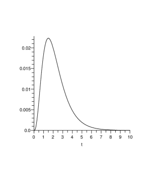
Figure 1: Plot of the function $\delta^{2}(t),$ $k=2.$

Limiting distribution of the statistic $D_{n}^{(2)}$ is unknown. Using the methods of Silverman [35], one can show that the $U$-empirical process

$$\eta_{n}^{(2)}(t)=\sqrt{n}\left(H_{n}^{(2)}(t)-G_{n}^{(2)}(t)\right),\ t\geq 0,$$

weakly converges in $D(0,\infty)$ as $n\to\infty$ to certain centered Gaussian process $\eta^{(2)}(t)$ with calculable covariance. Then the sequence of statistics $\sqrt{n}D_{n}^{(2)}$ converges in distribution to the random variable $\sup_{t\geq 0}|\eta^{(2)}(t)|$ but it is impossible to find explicitly its distribution. Hence it is reasonable to determine the critical values for statistics $D_{n}^{(2)}$ by simulation. Therefore in table 5 we give the critical values for Kolmogorov-type statistic for $k=2$ and $k=3$ obtained via simulation.

Table 5: Critical values for Kolmogorov type test $(n=100)$

$k$	$\alpha=0.1$	$\alpha=0.05$	$\alpha=0.01$	$\alpha=0.005$
2	0.305	0.313	0.328	0.334
3	0.446	0.455	0.473	0.481

The family of kernels $\{\Xi_{2}(X,Y;t)\},t\geq 0,$ is centered and bounded in the sense described in [27]. Applying the large deviation theorem for the supremum of the family of non-degenerate $U$- and $V$-statistics from [27] , we get the following result.

Theorem 3.

For $a>0$ it holds

$$\lim_{n\to\infty}n^{-1}\ln P_{H_{0}}(D_{n}^{(2)}>a)=-f_{2}(a),$$

where the function $f_{2}$ is continuous for sufficiently small $a>0,$ moreover

$$f_{2}(a)=(8\delta_{2}^{2})^{-1}a^{2}(1+o(1))\sim 5.595a^{2},\,\mbox{as}\,\,a\to 0.$$

3.1.1 Local Bahadur efficiency of the statistic $D_{n}^{(2)}$

According to Glivenko-Cantelli theorem for $V$-statistics [18] the limit in probability under the alternative for statistics $D_{n}^{(2)}$ is equal to

$$b_{D}^{(2)}(\theta)=\sup_{t\geq 0}|b_{D}^{(2)}(t,\theta)|=\sup_{t\geq 0}|P_{\theta}(\max(X,Y)<t)-P_{\theta}(X+\frac{Y}{2}<t)|.$$

Assuming the regularity of the alternative d.f., we can deduce

$$b_{D}^{(2)}(t,\theta)\sim 2\theta\int_{0}^{\infty}\xi_{2}(s;t)h(s)ds,\hskip 8.53581pt\theta\to 0,$$ (15)

where again $h(x)=\frac{\partial}{\partial\theta}g(x,\theta)\mid_{\theta=0}$ and $\xi_{2}(s;t)$ is the projection from (14).

We now proceed with calculation of local Bahadur efficiencies for our four alternatives.

For Makeham alternative from (15) we get that

$$b_{D}^{(2)}(t,\theta) \sim \theta\bigg{(}2\int_{0}^{t}F(t)e^{-s}(2-2e^{-s}-s)ds-\int_{0}^{t}F(2(t-s))e^{-s}(2-2e^{-s}-s)ds$$

$$-\int_{0}^{2t}F(t-s/2)e^{-s}(2-2e^{-s}-s)ds\bigg{)}$$

$$= \theta\big{(}\frac{2}{3}e^{-t}+(1-2t)e^{-2t}-2e^{-3t}+\frac{1}{3}e^{-4t}\big{)},\hskip 5.69054pt\theta\to 0.$$

Thus we have that

$$\sup_{t>0}b_{D}^{(2)}(t,\theta)=b_{D}^{(2)}(1.908,\theta)\sim 0.03055\;\theta,\,\theta\to 0.$$

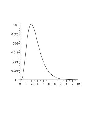
Figure 2: Plot of the function $b_{D}^{(2)}(t,\theta),\mbox{ Makeham alternative}$

The local exact slope of the sequence $D_{n}^{(2)}$ as $\theta\to 0$ satisfies

$$c_{D}^{(2)}(\theta)=(b^{(2)}_{D}(\theta))^{2}/(4\delta_{2}^{2})\sim 0.0104\;\theta^{2}.$$

Using $K_{1}(\theta)$ from (10), we get that the local BE is equal to

$$e^{B}(D^{(2)})=\lim_{\theta\to 0}\frac{c_{D}^{(2)}(\theta)}{2K_{1}(\theta)}\approx 0.125.$$

For other alternatives the calculations are similar. Therefore we omit them and present their local Bahadur efficiencies in table 6.

Table 6: Local Bahadur efficiency for the statistic $D_{n}^{(2)}.$

Alternative	Efficiency
Makeham	0.125
Weibull	0.092
Gamma	0.093
EMNW(3)	0.149

We see that the efficiencies are very low, considerably lower than in case of other tests of exponentiality based on characterizations with the exception, apparently, of [26]. Probably this is related to intrinsic properties of Arnold-Villasenor characterization.

3.2 Kolmogorov-type statistic $D_{n}^{(3)}$

For $k=3$ from (13) we get that the projection of the family of kernels $\Xi_{3}(X,Y,Z;t)$ is equal to

$$\xi_{3}(s;t) = \textbf{1}\{x<t\}\big{[}F^{2}(t)-F(2(t-x))+\frac{2}{3}F(3(t-x))\big{]}-\textbf{1}\{x<2t\}\big{[}\frac{1}{2}F(t-x/2)$$ (16)

$$- \frac{1}{6}F(3(t-x/2))\big{]}-\textbf{1}\{x<3t\}\big{[}\frac{2}{3}F(t-x/3)-\frac{1}{3}F(2(t-x/3))\big{]}.$$

Now we calculate the variances of these projections $\delta_{3}^{2}(t)$ under $H_{0}.$ We get that

$$\delta_{3}^{2}(t) = \frac{8}{15}e^{-t}+(\frac{1}{2}t-\frac{1}{24})e^{-2t}+(\frac{41}{9}-\frac{4}{3}t)e^{-3t}-\frac{179}{210}e^{-4t}+\frac{113}{210}e^{-5t}-\frac{419}{2520}e^{-6t}$$

$$- \frac{14}{15}e^{-3t/2}+\frac{122}{35}e^{-5t/2}-\frac{2}{3}e^{-7t/2}-\frac{2}{3}e^{-9t/2}-\frac{5}{7}e^{-5t/3}-\frac{5}{2}e^{-7t/3}+\frac{10}{7}e^{-8t/3}$$

$$- 4e^{-10t/3}-2e^{-11t/3}+2e^{-13t/3}.$$

The plot of this function is given in figure 3.

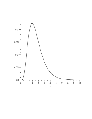
Figure 3: Plot of the function $\delta_{3}^{2}(t).$

Hence our family of kernels $\Xi_{3}(X,Y,Z;t)$ is non-degenerate in the sense described in [27] and

$$\delta_{3}^{2}=\sup_{t\geq 0}\delta_{3}^{2}(t)=0.02241.$$

Using the same reasoning as in the case $D_{n}^{(2)}$ we conclude that it is impossible to find explicitly the limiting distribution of the statistic $D_{n}^{(3)}$. The family of kernels $\{\Xi_{3}(X,Y,Z;t)\},$ $t\geq 0,$ is centered and bounded in the sense given in [27]. Applying the large deviation theorem for the supremum of the family of non-degenerate $U$- and $V$-statistics from [27], we get the following result.

Theorem 4.

For $a>0$ it holds

$$\lim_{n\to\infty}n^{-1}\ln P_{H_{0}}(D_{n}^{(3)}>a)=-f_{3}(a),$$

where the function $f$ is continuous for sufficiently small $a>0,$ moreover

$$f_{3}(a)=(18\delta_{3}^{2})^{-1}a^{2}(1+o(1))\sim 2.479a^{2},\,\mbox{as}\,\,a\to 0.$$

3.2.1 Local Bahadur efficiency of the statistic $D_{n}^{(3)}$

In this case the limit in probability under the alternative, according to Glivenko-Cantelli theorem for $V$-statistics [18], is equal to

$$b_{D}^{(3)}(\theta)=\sup_{t\geq 0}|b_{D}^{(3)}(t,\theta)|=\sup_{t\geq 0}|P_{\theta}(\max(X,Y,Z)<t)-P_{\theta}(X+\frac{Y}{2}+\frac{Z}{3}<t)|.$$

It is not difficult to show that $b_{D}(t,\theta)$ for regular alternatives satisfies the relation

$$b_{D}^{(3)}(t,\theta)\sim 3\theta\int_{0}^{\infty}\xi_{3}(s;t)h(s)ds,$$ (17)

where $h(x)=\frac{\partial}{\partial\theta}g(x,\theta)\mid_{\theta=0}$, and $\xi_{3}(s;t)$ is the projection from (16).

As in the previous sections we first calculate local BE for Makeham alternative. From (17) we get that

$$b_{D}^{(3)}(t,\theta) \sim \theta\bigg{(}\int_{0}^{t}\big{[}F^{2}(t)-F(2(t-s))+\frac{2}{3}F(3(t-s))\big{]}e^{-s}(2-2e^{-s}-s)ds$$

$$- \int_{0}^{2t}\big{[}\frac{1}{2}F(t-s/2)-\frac{1}{6}F(3(t-s/2))\big{]}e^{-s}(2-2e^{-s}-s)ds$$

$$- \int_{0}^{3t}\big{[}\frac{2}{3}F(t-s/3)-\frac{1}{3}F(2(t-s/3))\big{]}e^{-s}(2-2e^{-s}-s)ds\bigg{)}$$

$$= \theta\left(\frac{8}{5}e^{-t}+\big{(}\frac{9}{2}-6t\big{)}e^{-2t}-8e^{-3t}+2e^{-4t}-\frac{1}{10}e^{-6t}\right),\ \theta\to 0.$$

Therefore we get that

$$\sup_{t>0}b_{D}^{(3)}(t,\theta)=b_{D}^{(3)}(2.087,\theta)\sim 0.0602\;\theta.$$

Figure 4: Plot of the function $b_{D}^{(3)}(t,\theta),\mbox{ Makeham alteranative}$

The local exact slope of the sequence $D_{n}^{(3)}$ as $\theta\to 0$ satisfies

$$c_{D}^{(3)}(\theta)=(b^{(3)}_{D}(\theta))^{2}/(9\delta_{3}^{2})\sim 0.018\;\theta^{2},$$ (18)

and the local BE is equal to $e^{B}(D^{(3)})=0.216.$ Omitting again the detailed calculations, we present in table 7 the values of local Bahadur efficiency for our alternatives.

Table 7: Local Bahadur efficiency for statistic $D_{n}^{(3)}$

Alternative	Efficiency
Makeham	0.216
Weibull	0.152
Gamma	0.138
EMNW(3)	0.230

We see that these efficiencies are slightly better than in the previous case, but still rather low. In table 8 we present the simulated powers for our four alternatives. Again the simulations have been performed for $n=100$ with 10000 replicates.

Table 8: Simulated powers for statistic $D_{n}^{(k)}$

Alternative	$\theta$	$k$	$\alpha=0.05$	$\alpha=0.025$	$\alpha=0.01$
	0.5	2	0.0885	0.0472	0.0221
	0.5	3	0.1027	0.0609	0.0246
Makeham	0.5	4	0.1136	0.0681	0.0304
	0.25	2	0.0669	0.0315	0.0154
	0.25	3	0.0724	0.0399	0.0164
	0.25	4	0.0842	0.0475	0.0206
	0.5	2	0.6967	0.5721	0.4423
	0.5	3	0.8194	0.7431	0.6006
Weibull	0.5	4	0.8903	0.8287	0.7190
	0.25	2	0.2969	0.1964	0.1169
	0.25	3	0.3698	0.2745	0.1566
	0.25	4	0.4286	0.3308	0.2054
	0.5	2	0.4146	0.2901	0.1849
	0.5	3	0.5026	0.3887	0.2405
Gamma	0.5	4	0.5555	0.4433	0.3006
	0.25	2	0.1852	0.1135	0.0630
	0.25	3	0.2163	0.1437	0.0695
	0.25	4	0.2406	0.1628	0.0841
	0.5	2	0.7083	0.5769	0.4352
	0.5	3	0.7918	0.6936	0.5294
EMNW(3)	0.5	4	0.8409	0.7581	0.6121
	0.25	2	0.2080	0.1294	0.0718
	0.25	3	0.2456	0.1658	0.0817
	0.25	4	0.2849	0.1964	0.1083

4 Conditions of local asymptotic optimality

The efficiencies of our tests for standard alternatives are far from maximal ones. Nevertheless, there exist special alternatives (we call them most favorable) for which our sequences of statistics $I_{n}^{(k)}$ and $D_{n}^{(k)}$ are locally asymptotically optimal (LAO) in Bahadur sense (see general theory in [25, Ch.6]). In this section we describe the local structure of such alternatives, for which the given statistic has maximal possible local efficiency, so that the relation

$$c_{T}(\theta)\sim 2K(\theta),\,\theta\to 0,$$

holds (see [8], [25], [30], [28]). Such alternatives form the so-called domain of LAO for the given sequence of statistics $\{T_{n}\}$.

Denote by $\cal G$ the class of densities $g(\cdot\ ,\theta)$ with the d.f.’s $G(\cdot\ ,\theta)$. Define the functions

$$H(x)=\frac{\partial}{\partial\theta}G(x,\theta)\mid_{\theta=0},\quad h(x)=\frac{\partial}{\partial\theta}g(x,\theta)\mid_{\theta=0}.$$

Suppose also that for $G$ from $\cal G$ the following regularity conditions hold:

$$h(x)=H^{\prime}(x),\,x\geq 0,\quad\int_{0}^{\infty}h^{2}(x)e^{x}dx<\infty,$$

$$\frac{\partial}{\partial\theta}\int_{0}^{\infty}xg(x,\theta)dx\mid_{\theta=0}\ =\ \int_{0}^{\infty}xh(x)dx.$$

It is easy to show, see also [30], that under these conditions

$$2K(\theta)\sim\bigg{[}\int_{0}^{\infty}h^{2}(x)e^{x}dx-\bigg{(}\int_{0}^{\infty}xh(x)dx\bigg{)}^{2}\bigg{]}\theta^{2},\,\theta\to 0.$$

It can be shown that for the statistic (1) holds

$$b_{I}^{(k)}(\theta)\sim(k+1)\theta\int_{0}^{\infty}\psi_{k}(x)h(x)dx,\,\theta\to 0.$$

Let us introduce the auxiliary function

$$h_{0}(x)=h(x)-(x-1)\exp(-x)\int_{0}^{\infty}uh(u)du.$$ (19)

It is straightforward that

$$\int_{0}^{\infty}h^{2}(x)e^{x}dx-\bigg{(}\int_{0}^{\infty}xh(x)dx\bigg{)}^{2} = \int_{0}^{\infty}h_{0}^{2}(x)e^{x}dx,$$ (20)

$$\int_{0}^{\infty}\psi_{k}(x)h(x)dx = \int_{0}^{\infty}\psi_{k}(x)h_{0}(x)dx.$$

Consequently the local BE takes the form

$$e^{B}(I_{n}^{(k)}) = \lim_{\theta\to 0}\frac{(b_{I}^{(k)}(\theta))^{2}}{2(k+1)^{2}\Delta_{k}^{2}K(\theta)}$$

$$= \bigg{(}\int_{0}^{\infty}\psi_{k}(x)h_{0}(x)dx\bigg{)}^{2}/\bigg{(}\int_{0}^{\infty}\psi_{k}^{2}(x)e^{-x}dx\cdot\int_{0}^{\infty}h_{0}^{2}(x)e^{x}dx\bigg{)}.$$

The local Bahadur asymptotic optimality means that the expression on the right-hand side is equal to 1. It follows from Cauchy-Schwarz inequality (see also [28]) that this is satisfied if $h_{0}(x)=C_{1}e^{-x}\psi(x)$ for some constant $C_{1}>0,$ so that $h(x)=e^{-x}(C_{1}\psi(x)+C_{2}(x-1))$ for some constants $C_{1}>0$ and $C_{2}.$ Such distributions constitute the LAO domain in the class $\cal G$.

The simplest examples of such alternative densities $g(x,\theta)$ for small $\theta>0$ are given in table 9.

Table 9: Most favorable alternatives for $I_{n}^{(k)}.$

	Alternative density $g(x,\theta)$ as $\theta\to+0,\,x\geq 0$
$k=2$	$g(x,\theta)=e^{-x}\big{(}1+\frac{\theta}{3}(\frac{4}{3}e^{-x}-e^{-2x}-\frac{1}{2}e^{-x/2})\big{)}$
$k=3$	$g(x,\theta)=e^{-x}\big{(}1+\frac{\theta}{4}(\frac{5}{2}e^{-x}-3e^{-2x}+e^{-3x}-\frac{3}{8}e^{-x/2}-\frac{1}{3}e^{-x/3})\big{)}$

Let us now consider the Kolmogorov-type statistic (2). It can be shown that

$$b_{D}^{(k)}(\theta)\sim k\theta\int_{0}^{\infty}\xi_{k}(x;t)h(x)dx,\,\theta\to 0.$$

For $h_{0}(x)$ defined in (19), besides (20), also holds

$$\int_{0}^{\infty}\xi_{k}(x;t)h(x)dx=\int_{0}^{\infty}\xi_{k}(x;t)h_{0}(x)dx.$$

In this case the efficiency is equal to

$$e^{B}(D_{n}^{(k)}) = \lim_{\theta\to 0}\frac{(b^{(k)}_{D}(\theta))^{2}}{\sup_{t\geq 0}\left(2k^{2}\delta_{k}^{2}(t)\right)K(\theta)}$$

$$= \sup_{t\geq 0}\left(\int_{0}^{\infty}\xi_{k}(x;t)h_{0}(x)dx\right)^{2}/\ \sup_{t\geq 0}\left(\int_{0}^{\infty}\xi_{k}^{2}(x;t)e^{-x}dx\cdot\int_{0}^{\infty}h_{0}^{2}e^{x}dx\right).$$

From Cauchy-Schwarz inequality we obtain that efficiency is equal to 1 if $h(x)=e^{-x}\big{(}C_{1}\xi_{k}(x;t_{0})+C_{2}(x-1)\big{)}$ for $t_{0}={\rm argmax}_{t\geq 0}\delta_{k}^{2}(t)$ and some constants $C_{1}>0$ and $C_{2}.$ The alternative densities having such function $h(x)$ form the domain of LAO in the corresponding class.

The simplest examples are given in table 10. To facilitate the presentation, we denote:

$$t_{0} = \underset{t\geq 0}{\rm argmax}\bigg{(}\frac{1}{3}e^{-t}-\frac{5}{4}e^{-2t}-\frac{1}{3}e^{-3t}-\frac{1}{12}e^{-4t}-\frac{2}{3}e^{-3t/2}+2e^{-5t/2}+\frac{1}{2}te^{-2t}\bigg{)}\approx 1.502;$$

$$t_{1} = \underset{t\geq 0}{\rm argmax}\bigg{[}\frac{8}{15}e^{-t}+(\frac{1}{2}t-\frac{1}{24})e^{-2t}+(\frac{41}{9}-\frac{4}{3}t)e^{-3t}-\frac{179}{210}e^{-4t}+\frac{113}{210}e^{-5t}$$

$$- \frac{419}{2520}e^{-6t}-\frac{14}{15}e^{-3t/2}+\frac{122}{35}e^{-5t/2}-\frac{2}{3}e^{-7t/2}-\frac{2}{3}e^{-9t/2}-\frac{5}{7}e^{-5t/3}-\frac{5}{2}e^{-7t/3}$$

$$+ \frac{10}{7}e^{-8t/3}-4e^{-10t/3}-2e^{-11t/3}+2e^{-13t/3}\bigg{]}\approx 1.919.$$

Table 10: Most favorable alternatives for $D_{n}^{(k)}$

	Alternative densities $g(x,\theta)$ as $\theta\to+0,\,x\geq 0$
$k=2$	$g(x,\theta)=e^{-x}\bigg{(}1+\theta\cdot\textbf{1}\{x<t_{0}\}(1-e^{-t_{0}})-$
	$-\frac{1}{2}\theta\cdot\big{(}\textbf{1}\{x<t_{0}\}(1-e^{-2(t_{0}-x)})+\textbf{1}\{x<2t_{0}\}(1-e^{-(t_{0}-x/2)})\big{)}\bigg{)}$
$k=3$	$g(x,\theta)=e^{-x}\bigg{(}1+\theta\cdot\textbf{1}\{x<t_{1}\}\big{[}(1-e^{-t_{1}})^{2}+e^{-2(t_{1}-x)}-\frac{2}{3}e^{-3(t_{1}-x)}-\frac{1}{3}\big{]}$
	$-\frac{1}{3}\theta\cdot\textbf{1}\{x<2t_{1}\}\big{[}1-\frac{3}{2}e^{-(t_{1}-x/2)}+\frac{1}{2}e^{-3(t_{1}-x/2)}\big{]}$
	$-\frac{1}{3}\theta\cdot\textbf{1}\{x<3t_{1}\}\big{[}1-2e^{-(t_{1}-x/3)}+e^{-2(t_{1}-x/3)}\big{]}\bigg{)}$

5 Discussion

In this paper we have proposed two families of asymptotic tests of exponentiality based on recent characterization of exponentiality by Arnold and Villasenor [4]. The integral test statistics $I_{n}^{(k)}$ are asymptotically normal and have reasonably simple form which can be easily computed for small $k.$ They are consistent for many common alternatives and have local Bahadur efficiency around 0.5 - 0.7. There exist also special (most favorable) alternatives described in the section 4 for which the integral statistics are locally asymptotically optimal in this sense.

We also obtained via simulation the power of new integral statistics for chosen alternatives. In theory, the ordering of tests by power is linked more closely to Hodges-Lehmann efficiency [25], and should not coincide with the ordering by local Bahadur efficiency. Nevertheless, we observe tolerable correspondence of test quality according to both criteria with the exception of Gamma and Weibull distribution. In whole we can recommend new integral tests of exponentiality as additional and auxiliary tests of exponentiality, especially when one is trying to reject exponentiality in a specific example using a ”battery” of statistical tests.

In the case of Kolmogorov type tests the values of local Bahadur efficiency turned out to be rather low for common alternatives, and the simulated powers (which are slightly more optimistic) do not change somewhat disadvantageous regard to new tests of exponentiality of supremum type. Probably it is closely related to intrinsic properties of Arnold-Villasenor characterization. However, even these tests, in virtue of their consistency, can be of some use in statistical research, especially when the (unknown) alternative is close to the most favorable one.

6 Acknowledgement

The authors express their deep gratitude to Prof. George Yanev who kindly sent them the files of his papers [11] and [37].

References

- [1]
- [2] I. Ahmad, I.Alwasel, A goodness-of-fit test for exponentiality based on the memoryless property, J. Roy. Stat. Soc. B 61, Pt.3 (1999), 681 – 689. doi: 10.1111/1467-9868.00200.
- [3] M. Ahsanullah, G.G. Hamedani, Exponential Distribution: Theory and Methods, NOVA Science, New York, 2010.
- [4] B.C. Arnold, J.A. Villasenor, Exponential characterizations motivated by the structure of order statistics in samples of size two, Stat. Probab. Lett. 83(2) (2013), 596 – 601. doi: 10.1016/j.spl.2012.10.028.
- [5] J.E. Angus, Goodness-of-fit tests for exponentiality based on a loss-of-memory type functional equation, J. Stat. Plann. Infer. 6(3) (1982), 241 – 251. doi: 10.1016/0378-3758(82)90029-5.
- [6] S. Asher, A survey of tests for exponentiality, Commun. Stat.- Theor. Meth. 19(5) (1990), 1811 – 1825. doi: 10.1080/03610929008830292.
- [7] R.R. Bahadur, Stochastic comparison of tests, Ann. Math. Stat. 31(2) (1960), 276 – 295. doi: 10.1214/aoms/1177705894.
- [8] R.R. Bahadur, Some limit theorems in statistics, SIAM, Philadelphia, 1971.
- [9] N. Balakrishnan, A. Basu, The exponential distribution: theory, methods and applications, Gordon and Breach, Langhorne, PA, 1995.
- [10] L. Baringhaus, N. Henze, Tests of fit for exponentiality based on a characterization via the mean residual life function, Stat. Papers 41 (2000), 225 – 236. doi: 10.1007/BF02926105.
- [11] S. Chakraborty, G.P. Yanev, Characterization of exponential distribution through equidistribution conditions for consecutive maxima, J. Stat. Appl. Prob. 2(3) (2013), 237 – 242. doi: 10.12785/jsap/020306.
- [12] A. DasGupta, Asymptotic Theory of Statistics and Probability, Springer, New York, 2008.
- [13] K.A. Doksum, B.S. Yandell, Tests of exponentiality, Handbook of Statistics 4, 1985, 579 – 612.
- [14] R. Helmers, P. Janssen, R. Serfling, Glivenko-Cantelli properties of some generalized empirical DF’s and strong convergence of generalized L-statistics, Probab. Theor. Rel. Fields 79 (1988), 75 – 93. doi: 10.1007/BF00319105.
- [15] N. Henze, S. Meintanis, Goodness-of-fit tests based on a new characterization of the exponential distribution, Commun. Stat. Theor. Meth. 31(9) (2002), 1479 – 1497. doi: 10.1081/STA-120013007.
- [16] W. Hoeffding, A class of statistics with asymptotically normal distribution, Ann. Math. Stat. 19 (1948), 293 – 325. doi: 10.1214/aoms/1177730196.
- [17] H.M. Jansen van Rensburg, J.W.H. Swanepoel, A class of goodness-of-fit tests based on a new characterization of the exponential distribution, J. Nonparam. Stat. 20(6) (2008), 539 – 551. doi: 10.1080/10485250802280242.
- [18] P.L. Janssen, Generalized empirical distribution functions with statistical applications, Limburgs Universitair Centrum, Diepenbeek, 1988.
- [19] V. Jevremović, A note on mixed exponential distribution with negative weights, Stat. Probab. Lett. 11(3) (1991), 259-265. doi: 10.1016/0167-7152(91)90153-I.
- [20] V.S. Korolyuk, Yu.V. Borovskikh, Theory of -statistics, Kluwer, Dordrecht, 1994.
- [21] H.L. Koul, A test for new better than used, Commun. Stat. Theor. Meth. 6(6) (1977), 563 – 574. doi: 10.1080/03610927708827514.
- [22] H.L. Koul, Testing for new is better than used in expectation, Commun. Stat. Theor. Meth. 7(7) (1978), 685 – 701. doi: 10.1080/03610927808827658.
- [23] V.V. Litvinova, Asymptotic properties of goodness-of-fit and symmetry tests based on characterizations, Ph.D. thesis, Saint-Petersburg University, 2004.
- [24] P. Nabendu, J. Chun, R. Crouse, Handbook of exponential and related distributions for engineers and scientists, Chapman and Hall, 2002.
- [25] Y. Nikitin, Asymptotic efficiency of nonparametric tests, Cambridge University Press, New York, 1995.
- [26] Ya. Yu. Nikitin, Bahadur efficiency of a test of exponentiality based on a loss of memory type functional equation, J. Nonparam. Stat. 6(1) (1996), 13 – 26. doi: 10.1080/10485259608832660.
- [27] Ya. Yu. Nikitin, Large deviations of -empirical Kolmogorov-Smirnov tests and their efficiency, J. Nonparam. Stat. 22(5) (2010), 649 – 668. doi: 10.1080/10485250903118085.
- [28] Ya. Yu. Nikitin, I. Peaucelle, Efficiency and local optimality of distribution-free tests based on - and - statistics, Metron LXII (2004), 185 – 200.
- [29] Ya. Yu. Nikitin, E.V. Ponikarov, Rough large deviation asymptotics of Chernoff type for von Mises functionals and -statistics, Proceedings of the St. Petersburg Mathematical Society 7, 1999, 124–167. English translation in AMS Translations ser.2 203, 2001, 107 – 146.
- [30] Ya. Yu. Nikitin, A.V. Tchirina, Bahadur efficiency and local optimality of a test for the exponential distribution based on the Gini statistic, Stat. Methods Appl. 5(1) (1996), 163 – 175. doi: 10.1007/BF02589587.
- [31] Ya. Yu. Nikitin, K. Yu. Volkova, Asymptotic efficiency of exponentiality tests based on order statistics characterization, Georgian Math. J. 17 (2010), 749 – 763. doi: 10.1515/GMJ.2010.034.
- [32] H.A. Noughabi, N.R. Arghamia, Testing exponentiality based on characterizations of the exponential distribution, J. Stat. Comput. Sim. 81(11) (2011), 1641 – 1651. doi: 10.1080/00949655.2010.498373.
- [33] R.F. Rank, Statistische Anpassungstests und Wahrscheinlichkeiten grosser Abweichungen, Dr. rer. nat. genehmigte Dissertation, Hannover, 1999.
- [34] J.S. Rao, E. Taufer, The use of Mean Residual Life to test departures from Exponentiality, J. Nonparam. Stat. 18(3) (2006), 277 – 292. doi: 10.1080/10485250600759454.
- [35] B.W. Silverman, Convergence of a class of empirical distribution functions of dependent random variables, Ann. Prob. 11(3) (1983), 745 – 751. doi: 10.1214/aop/1176993518.
- [36] H.S. Wieand, A condition under which the Pitman and Bahadur approaches to efficiency coincide, Ann. Stat. 4 (5) (1976), 1003 – 1011. doi: 10.1214/aos/1176343600.
- [37] G.P. Yanev, S. Chakraborty, Characterizations of exponential distribution based on sample of size three, Pliska Stud. Math. Bulgar. 23 (2013), 237 - 244.