Exotic electron states and tunable magneto-transport in a fractal Aharonov-Bohm interferometer

Abstract

A Sierpinski gasket fractal network model is studied in respect of its electronic spectrum and magneto-transport when each ‘arm’ of the gasket is replaced by a diamond shaped Aharonov-Bohm interferometer, threaded by a uniform magnetic flux. Within the framework of a tight binding model for non-interacting, spinless electrons and a real space renormalization group method we unravel a class of extended and localized electronic states. In particular, we demonstrate the existence of extreme localization of electronic states at a special finite set of energy eigenvalues, and an infinite set of energy eigenvalues where the localization gets ‘delayed’ in space (staggered localization). These eigenstates exhibit a multitude of localization areas. The two terminal transmission coefficient and its dependence on the magnetic flux threading each basic Aharonov-Bohm interferometer is studied in details. Sharp switch on- switch off effects that can be tuned by controlling the flux from outside, are discussed. Our results are analytically exact.

I Introduction

When an electron goes round a closed loop that traps a magnetic flux $\Phi$, its wave function gains a phase $\phi=2\pi\Phi/\Phi_{0}$, where, $\Phi_{0}=hc/e$ is the fundamental flux quantum. This simple sentence is at the heart of the path-breaking Aharonov-Bohm (AB) effect aharonov ; washburn ; markus1 ; markus2 ; markus3 that has led to an extensive research in the so called AB interferometry which dominated the physics, both experiments and theory, in mesoscopic dimensions over the past couple of decades yacoby1 ; yacoby2 ; casse ; kubala ; kim ; kobayashi ; aharony1 ; aharony2 ; aharony3 ; benjamin ; aldea ; forster ; aharony4 ; camino ; aharony5 ; kubo1 ; urban ; kubo2 .

While recent experiments by Yamamoto et al. yamamoto has inspired more experiments on quantum transport in AB interferometers aharony6 , the earlier theoretical model studies have also played an instrumental role in understanding the basic features of electronic states and coherent transport in quantum network models in the mesoscopic or nano-dimensional systems casse ; kubala ; kim ; kobayashi ; aharony1 ; aharony2 ; aharony3 ; benjamin ; aldea ; forster ; aharony4 ; camino ; aharony5 ; kubo1 ; urban ; kubo2 . The present day advanced growth, fabrication and lithographic techniques have opened up the possibility of artificial, tailor made lattice structures using quantum dots (QD) or Bose-Einstein condensates (BEC) with tremendous potential for application in device technologies. Needless to say, this has stimulated a considerable volume of theoretical research even in model quantum networks with a complex topological character andrade ; cardoso ; oliviera .

In this communication, inspired by the present scenario of theory and experiments in AB interferometry, we examine the spectral and transport properties of a quantum network in which diamond shaped AB interferometers are arranged in a Sierpinski gasket (SPG) geometry (Fig. 1). The SPG geometry is already an extensively studied example of a finitely ramified fractal network  domany ; rammal ; banavar ; wang , exhibiting exotic electronic spectrum. Apart from it, it has also been experimentally exploited to observe dimensionality crossover in superconducting wire networks gordon , as well as considered for modeling photonic wave guide networks li ; cooley . We revisit it in the shape of an AB interferometric arrangement of model nanorings.

In our work, each elementary interferometer is pierced by a uniform magnetic field applied perpendicular to the plane of the diamond plaquette, and traps a flux $\Phi$.

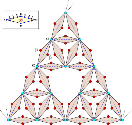
Figure 1: (Color online) Schematic view of a part of an infinite fractal Aharonov-Bohm (AB) interferometer formed by arranging diamond shaped closed loops on a Sierpinski gasket (SPG) matrix. In the inset we have shown a basic plaquette where each arm of the diamond loop contains $N$ number of sites in between two vertices. A uniform magnetic flux $\Phi$ pierces every closed diamond shaped loop.

Such diamond shaped interferometers have previously been studied as the minimal models of bipartite structures having nodes with different coordination numbers, and representing a family of itinerant geometrically frustrated electronic systems  vollhardt ; lopes1 ; lopes2 . Other studies include the problem of electron localization in the presence of spin-orbit interaction bercioux , a flux-induced semiconducting behavior sil , quantum level engineering for AB cages movilla or, as models of spin filters aharony7 ; aharony8 . Placed in a motif of a recursively grown, self-similar, hierarchical pattern of the SPG, such a fractal AB interferometer gives us an opportunity to critically examine the interplay of quantum interference and lattice topology in the light of recent developments in the subject.

As a first step in this direction, we examine the spectral properties of non-interacting, spinless electrons described in a tight binding formalism. Using an exact real space renormalization group (RSRG) decimation scheme we show that, the spectrum of such an AB interferometer consists of an infinity of extended and localized eigenfunctions induced by the topology of the nanocluster. Localized states can belong to at least a couple different categories, and can be made to occupy any part of the energy spectrum by tuning the out of plane magnetic field. For one class of localized eigenstates, the onset of localization can be ‘delayed’ (in space) at will, by extracting the corresponding energy at any desired length scale. These are called the staggered localized states, and can be placed at any desired part of the energy spectrum by controlling the magnetic flux. This latter control over position of the eigenstates of course, is true for all kinds of states.

In addition, the magnetic flux can be used to control the width of the gaps in the spectrum, and for special value of flux $\Phi=\Phi_{0}/2$, the entire spectrum is shown to collapse into extremely localized eigenstates, a fact known as the AB-caging and pioneered by Vidal et al. vidal1 ; vidal2 ; vidal3 ; vidal4 .

In what follows we describe our findings. In section II we describe the Hamiltonian and the RSRG scheme. Section III contains a discussion of the density of states and the nature of the eigenfunctions, and in section IV we present the transport calculations. Finally, in section V we draw our conclusions.

II The beginning

We refer to Fig. 1. A basic diamond AB interferometer is shown in the inset. Each arm of the diamond contains $N$ number of single level QD’s  kubala between the vertices, so that the total number of dots contained in adiamond is $4N+4$. A magnetic flux $\Phi$ pierces each plaquette, and we restrict electron hopping only along the arm of a diamond. Spinless, non-interacting electrons are described by the Hamiltonian,

$${\bm{H}}=\sum_{i}\epsilon_{i}c_{i}^{\dagger}c_{i}+\sum_{\langle ij\rangle}\left[t_{ij}e^{i\phi_{ij}}c_{i}^{\dagger}c_{j}+h.c.\right]$$ (1)

$\epsilon_{i}$ is the on-site potential at each QD-location, which we assume to be constant. That is, $\epsilon_{i}=\epsilon$ at every vertex $i$. The nearest neighbor hopping integral $t_{ij}$ is associated with a typical AB-phase $\phi_{ij}=(2\pi/\Phi_{0})\int_{i}^{j}\vec{A}\cdot d\vec{r}$, $\vec{A}$ being the vector potential. This phase factor breaks the time reversal symmetry of electron- hopping along the arms of the interferometer.

Using the set of difference equations satisfied by the electrons, viz.,

$$(E-\epsilon_{i})\psi_{i}=\sum_{j}t_{ij}e^{i\phi_{ij}}\psi_{j}$$ (2)

we first renormalize each diamond plaquette shown in the inset of Fig. 1 into an elementary diamond having just four sites. The renormalized plaquettes are then joined recursively to generate a SPG geometry, as shown. Two kinds of sites are generated for an infinite geometry. These sites are marked by the cyan dots ($\alpha$) and red dots ($\beta$). The coordination numbers for the vertices $\alpha$ and $\beta$ are eight and two respectively. On renormalization of the elementary plaquettes (inset), the effective on-site potentials at these two sites are given by,

$$\epsilon_{\alpha}=\epsilon+8t\dfrac{U_{N-1}(x)}{U_{N}(x)}$$ (3)

$$\epsilon_{\beta}=\epsilon+2t\dfrac{U_{N-1}(x)}{U_{N}(x)}$$

the inter-vertex hopping integral acquires a phase, and is given by,

$$t_{F}=t\dfrac{e^{i\phi(N+1)}}{U_{N}(x)}$$ (4)

in the forward direction and, the backward hopping is $t_{B}=t_{F}^{*}$. Here, $\phi=2\pi\Phi/(N+1)\Phi_{0}$, $U_{N}(x)$ is the $N$-th order Chebyshev polynomial of second kind, and $x=(E-\epsilon)/2t$. The familiar SPG network of triangles is easily restored from Fig. 1 by joining the $\alpha$-sites (cyan dots), and ‘eliminating’ the $\beta$-sites (red dots). This leads to the usual triangular SPG geometry (shown by blue dotted lines in Fig. 1) with only one kind of ‘bulk’ sites having an effective on-site potential,

$$\tilde{\epsilon}=\epsilon_{\alpha}+\dfrac{8t^{2}}{(E-\epsilon_{\beta})}$$ (5)

and an effective nearest neighbor hopping integral along an arm of the SPG geometry (blue dotted lines) given by,

$$\tilde{t}=\dfrac{2t^{2}}{(E-\epsilon_{\beta})}\cos\left(\dfrac{\pi\Phi}{\Phi_{0}}\right)$$ (6)

We shall now exploit Eq. (5) and Eq. (6) to extract information about the spectrum, eigenstates and transport provided by such a hierarchical AB interferometer.

III The RSRG scheme and spectral analysis

An elementary SPG triangle is shown in Fig. 2. Both the solid black and grey circles have the same on-site potential $\tilde{\epsilon}$. The first step is to decimate out the grey circles in Fig. 2

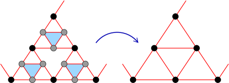
Figure 2: (Color online) Decimation renormalization scheme of a basic Sierpinski geometry. The grey shaded circles are ‘eliminated’ to generate the next re-scaled version.

to obtain a renormalized SPG geometry. Only the bulk sites have been shown. The renormalized on-site potential and the nearest neighbor hopping integrals are given by arunava ,

$$\tilde{\epsilon}_{n+1}=\tilde{\epsilon}_{n}+\dfrac{4\tilde{t}_{n}^{2}(E-\tilde{\epsilon}_{n})}{(E-\tilde{\epsilon}_{n})^{2}-(E-\tilde{\epsilon}_{n})\tilde{t}_{n}-2\tilde{t}_{n}^{2}}$$ (7)

$$\tilde{t}_{n+1}=\dfrac{2\tilde{t}_{n}^{3}+(E-\tilde{\epsilon}_{n})\tilde{t}_{n}^{2}}{(E-\tilde{\epsilon}_{n})^{2}-(E-\tilde{\epsilon}_{n})\tilde{t}_{n}-2\tilde{t}_{n}^{2}}$$

In Eq. (7) $n$ refers to the ‘stage’ of renormalization. Therefore, $\tilde{\epsilon}_{0}=\tilde{\epsilon}$, and $\tilde{t}_{0}=\tilde{t}$ as given by Eq. (5) and Eq. (6) respectively.

To get an overall view about the flux dependence of the distribution of eigenvalues, we present an energy versus flux diagram for an infinite SPG-AB interferometer by evaluating the local Green’s function $G_{\alpha}(E)$ at the $\alpha$-sites. The simplest picture for the case $N=0$ is shown in Fig. 3. The elementary diamond AB interferometer (inset of Fig. 1) now contains just four sites at the vertices. The basic building blocks now resemble the $AB_{2}$ structural unit used by Lopes et al. lopes2 in describing their geometrically frustrated systems.

The spectrum of the SPG-AB interferometer with $N=0$ exhibits a periodicity of $2\Phi_{0}$ (Fig. 3).

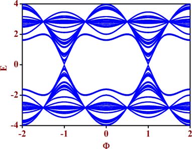
Figure 3: (Color online) Flux dependence of energy eigenvalues of an infinite $N=0$ AB interferometer based on a Sierpinski gasket geometry.

There is a tendency of clustering of the eigenvalues towards the edges of the spectrum as is evident from the $E$-$\Phi$ diagram. Multiple band crossings are observed and the spectrum exhibits kind of a zero band gap semiconductor like behavior, mimicking a Dirac point as seen in graphene, at $\Phi=\pm\Phi_{0}$. The central gap gets gradually filled up by more eigenstates, and the $E$-$\Phi$ contours get more flattened up as $N$ increases. The spectrum at $\Phi=\Phi_{0}/2$ consists of only a discrete set of points. This is the case of extreme localization, and happens for any value of $N$, the number of eigenvalues in this discrete set depending upon the value of $N$. We shall come back to it later. Let us now discuss case by case.

III.1 Extended States

It is simple to verify from Eq. (7) that, if we set $E=\tilde{\epsilon}_{n}$, then $\tilde{\epsilon}_{n+1}=\tilde{\epsilon}_{n}$ and, $\tilde{t}_{n+2}=-\tilde{t}_{n+1}=\tilde{t}_{n}$ for all subsequent values of $n$ arunava . If a non-zero value of the hopping integral persists at all stages of renormalization, it clearly indicates that the amplitudes of the wave function have a non-zero overlap between neighboring sites at that scale of length. The corresponding energy eigenvalue will thus be of an extended character. Depending on the number of QD’s in each diamond AB interferometer, the equation $E-\tilde{\epsilon}_{n}=0$ will yield a finite number of roots. Each real root will then correspond to an eigenvalue of the infinite SPG-AB interferometer for which the parameter space ($\tilde{\epsilon}_{n}$,$\tilde{t}_{n}$) will exhibit a two cycle fixed point,

$$(\tilde{\epsilon}_{n},\tilde{t}_{n})\rightarrow(\tilde{\epsilon}_{n+1},-\tilde{t}_{n+1})\rightarrow(\tilde{\epsilon}_{n+2},\tilde{t}_{n+2})$$ (8)

The cyclic behavior will set in at a desired value of the RSRG stage $n$, at which the roots are extracted. If we make $N\rightarrow\infty$, the roots (eigenvalues) will be densely packed in the energy spectrum, forming a quasi-continuum.

For example, with $N=0$, if we set $E=\tilde{\epsilon}_{0}=\tilde{\epsilon}=\epsilon+8t^{2}/(E-\epsilon)$ at the bare length scale ($n=0$), we get two eigenvalues viz., $E=\epsilon\pm 2\sqrt{2}t$ which will correspond to extended eigenstates in an infinite geometry. The parameter space starts exhibiting a two cycle behavior right from the RSRG step $n=1$ onward. These eigenvalues are independent of the flux $\Phi$. The eigenvalues obtained from the equation $E=\tilde{\epsilon}_{1}$ become functions of the flux $\Phi$. For each of them, at any value of the flux $\Phi$, excluding the value $\Phi=\Phi_{0}/2$, the hopping integral $\tilde{t}_{n}$ starts flowing into a two-cycle fixed point for $n\geq 2$.

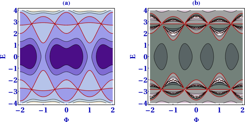
Figure 4: (Color online) Contour plots of the functions (a) $\mathcal{F}_{1}(E,\Phi)=E-\tilde{\epsilon}_{1}$ and (b) $\mathcal{G}_{1}(E,\Phi)=E-\tilde{\epsilon}_{1}-\tilde{t}_{1}$. The red contours in each case indicate a continuous distribution of energy and flux for which one can have extended (in (a)) and the staggered localized eigenstates (in (b)) on a one step renormalized lattice.

Continuing this argument it is possible to discern a countably infinite number of discrete eigenvalues in the limit $n\rightarrow\infty$, and all corresponding to extended eigenstates in such a non-translationally invariant interferometer arrangement. By tuning the magnetic flux appropriately, it is possible to ‘place’ such eigenvalues at any desired location in the energy spectrum. Such extended eigenstates can, in principle, lie arbitrarily close to the neighboring localized states. Thus, by controlling the external magnetic field it may be possible to achieve sharp switch on-switch off effects over arbitrarily small energy intervals.

In Fig. 4(a) we present the contour plot of the function $\mathcal{F}_{1}(E,\Phi)=E-\tilde{\epsilon}_{1}$. If we progress along the red lines we can have a continuous distribution of the energy $E$ and the magnetic flux $\Phi$ for which extended states are obtained from a one-step renormalized SPG-AB interferometer. The immediate neighborhood of the red contour at any place of the plot is largely deviated from the desired result $\mathcal{F}_{1}(E,\Phi)=0$, indicating that the extended states are isolated. Extended states arising from the other scales of length ($n\geq 2$) as solutions of the equation $\mathcal{F}_{n}(E,\Phi)=0$ get densely packed in the energy spectrum, but do not form a continuum.

III.2 Localization of Eigenfunction

Absence of any kind of translational invariance makes the appearance of localized eigenstates a natural phenomenon. We highlight below some interesting variations of these localized states.

III.2.1 Staggered Localization

Let’s refer back to the set of recursion relations Eq. (7). The roots of the equation $\mathcal{G}_{n}(E,\Phi)=E-\tilde{\epsilon}_{n}-\tilde{t}_{n}=0$ yield an interesting result in the sense that, for any value of energy extracted out of this equation, the hopping integral $\tilde{t}$ remains non-zero upto the $(n+1)$-th stage of renormalization, and starts to decay beyond the $(n+1)$-th RSRG step. This implies that for such energy values the amplitudes of the corresponding wave function have a non-trivial distribution over a cluster of vertices of the SPG-AB inteferometer. The size of the cluster increases with increasing value of the RSRG step $n$ from which the roots are extracted.

That such energies indeed belong to the spectrum, has been verified by exhaustive calculation of the density of states. As the SPG geometry is scaled by a scale factor of three, the size of the cluster over which the amplitudes of the wave functions have a non-trivial distribution typically gets enlarged in proportion of $3^{n}$. Clusters accommodating the non-trivial distribution of wave functions get decoupled from each other (or, remain very weakly coupled at the most) beyond a certain scale in such cases.

Since the hopping integral $\tilde{t}$ starts flowing to zero beyond the $(n+1)$-th stage, such wave functions are indeed localized, but the localization-area increases with increasing value of $n$. In principle, for all such energy eigenvalues extracted out of the equation $\mathcal{G}_{n}(E,\Phi)=E-\tilde{\epsilon}_{n}-\tilde{t}_{n}=0$ in the limit $n\rightarrow\infty$, we encounter a countable infinity of eigenfunctions which span the infinitely large interferometer and yet retain a localized character. The choice of the RSRG iteration index $n$ thus allows one to ‘delay’ (in space) the onset of localization. We name such an effect as staggered localization biplab1 .

Contrary to the case of the extended states, the eigenvalues corresponding to the staggered localized states depend on the flux $\Phi$ from the beginning ($n=0$ level), and the staggered localization can thus be controlled, at any scale of length, to occupy any desired place in the energy spectrum. In Fig. 4(b) we show the contour plot of the function $\mathcal{G}_{1}(E,\Phi)$ which bring out the location of the energy eigenvalues corresponding to the staggered localized states, as marked by the red contours. Such states are again isolated, and the number of such states increases with increasing value of $n$ (and of course, with the number $N$ of QD’s sitting on the arms of the elementary diamond interferometer).

III.2.2 Localized Edge States

Existence of localized edge states (LES) in case of an ordinary SPG network was pointed out in the pioneering work by Domany et al. domany . We discuss it in terms of the recursion relations Eq. (7), and unravel the link with the staggered localized states discussed above.

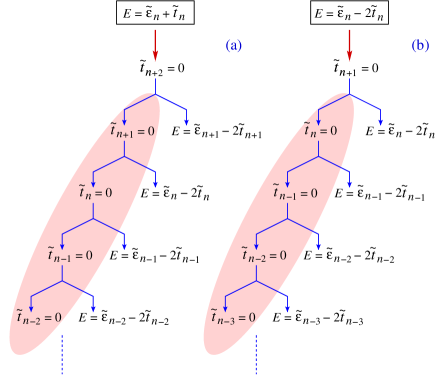
Figure 5: (Color online) The genealogical trees for the (a) staggered localized states and (b) edge localized states of the SPG-AB interferometer. In both the figures the highlighted branches of the tree correspond to the extreme localization.

Let us set $E=\tilde{\epsilon}_{n+1}-2\tilde{t}_{n+1}$. This immediately makes $\tilde{t}_{n+2}=0$. Then, trivially, hopping integrals at all successive stages of renormalization become zero, indicating that these eigenvalues correspond to sharply localized states, and as argued by Domany et al., they represent the so called edge states. It is easy to work out using Eq. (7), that with the above choice of energy $E$, one arrives at an equation,

$$\left[(E-\tilde{\epsilon}_{n})^{2}-4\tilde{t}_{n}^{2}\right](E-\tilde{\epsilon}_{n}-\tilde{t}_{n})=0$$ (9)

Clearly, the eigenvalues giving rise to the staggered localization, viz., $E=\tilde{\epsilon}_{n}+\tilde{t}_{n}$ are all embedded in the cluster of eigenvalues obtained from Eq. (9).

Setting $E=\tilde{\epsilon}_{n}-2\tilde{t}_{n}$ yields two branches of solutions. One gets either $\tilde{t}_{n}=0$, or $E=\tilde{\epsilon}_{n}-2\tilde{t}_{n}$. Each branch bifurcates into two similar branches as one climbs down the genealogical tree of solutions (Fig. 5(b)). If one sticks to the shaded branch only, one encounters either a situation where the hopping integral is zero from the very beginning. This is a trivial situation, except in one case of the so called extreme localization, as will be discussed immediately after this. The non-shaded branch keeps on generating a multitude of the edge-localized eigenstates, in the same spirit as discussed by Domany et al. domany .

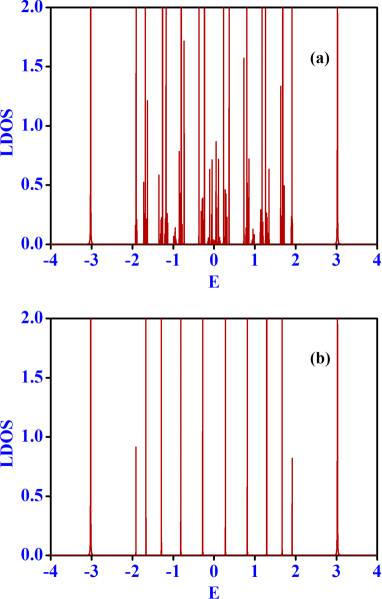
Figure 6: (Color online) Local density of states at the bulk ($\alpha$-type) sites of the SPG-AB interferometer with $N=5$. The panels exhibit results for (a) $\Phi=0$, and (b) for $\Phi=\Phi_{0}/2$. In the latter case, the entire spectrum consists of only such extremely localized states. We have selected $\epsilon=0$ and $t=1$, and energy is measured in units of $t$.

For each root steming from this branch at the $n$-th level, the hopping integral drastically drops to zero at the $(n+1)$-th stage of renormalization in contrast to the case of staggered localization.

Interestingly, the genealogical tree of the staggered localized eigenstates resulting from the equation $E=\tilde{\epsilon}_{n}+\tilde{t}_{n}$ yields, as a branch, the edge localized states, as is evident from Fig. 5(a). This indicates an interesting grouping of the two different kinds of localization, namely the staggered and the edge ones. The tuning of the flux can make this grouping take place at any desired part of the energy spectrum. The extreme localization branch along which $\tilde{t}_{n}=0$ for any value of $n$, is also obtained as part of the solution of the equation $E=\tilde{\epsilon}_{n}+\tilde{t}_{n}$.

The subsection of the roots extracted from the equation $E-\tilde{\epsilon}_{n}-2\tilde{t}_{n}=0$ is ruled out as exhaustive calculation of the density of states indicate that such roots are not part of the energy spectrum.

III.2.3 Extreme Localization

From Eq. (7) it is clear that the eigenvalues corresponding to the ‘extended’ eigenstates extracted from the equation $E=\tilde{\epsilon}_{0}$ are independent of the magnetic flux threading an elementary diamond interferometer. Interestingly, if one sets the magnetic flux $\Phi=\Phi_{0}/2$, these extended states drastically get converted into a set of extremely localized eigenstates in the spirit of the AB cages first pointed out by Vidal et al. vidal1 ; vidal2 ; vidal3 . The dynamics of the electron is confined within clusters of finite size only in all such cases. At half flux quantum, because of the presence of the cosine term in Eq. (6) the effective hopping integral connecting the vertices of the SPG vanishes confining the amplitudes of the wave function in local cages, the cages being distributed and decoupled from each other all over the SPG geometry.

Before ending this section, we discuss the general shape of the density of states of an SPG-AB interferometer for $N\neq 0$. In Fig. 6 we present the local density of states (LDOS) at the bulk ($\alpha$, cyan) sites of the AB-SPG interferometer shown in Fig. 1. Each arm of the basic diamond plaquette now contains $N=5$ QD’s. The spectrum shown in Fig. 6(a) shows a dense clustering of eigenstates which is a mixture of extended, staggered localized, and the edge states in the absence of a magnetic flux. The spectrum gradually thins out as $\Phi\rightarrow\Phi_{0}/2$, and collapses into a set of extremely localized states only as $\Phi=\Phi_{0}/2$.

IV Two-terminal transmission characteristics

To get an overview about the nature of the transmittance of such fractal network we have computed the two-terminal transmission characteristics of a finite generation system. The procedure is standard and is often used to evaluate the transmission coefficient of such hierarchical fractal structures biplab1 ; biplab2 . We clamp the system in between two semi-infinite periodic leads, the so called ‘source’ and the ‘drain’. The leads are characterized by a constant on-site potential ${\mathcal{U}}_{L}$ and a constant hopping integral ${\mathcal{T}}_{L}$ in between the atomic sites of the leads. The finite sized network sandwiched in between the two ordered leads is then successively renormalized to reduce it to an effective di-atomic system biplab2 . The transmission coefficient of the lead-network-lead system is given by a well-known formula liu ,

$$T=\dfrac{4\sin^{2}ka}{|\mathcal{A}|^{2}+|\mathcal{B}|^{2}}$$ (10)

$$\text{with,}\quad\mathcal{A}=[(M_{12}-M_{21})+(M_{11}-M_{22})\cos ka]$$

$$\text{and}\quad\mathcal{B}=[(M_{11}+M_{22})\sin ka]$$

where, $M_{ij}$ refer to the dimer-matrix elements, written appropriately in terms of the on-site potentials of the final renormalized left (L) and right (R) atoms $\epsilon_{L}$ and $\epsilon_{R}$ respectively, and the renormalized hopping between them. $\cos ka=(E-{\mathcal{U}}_{L})/2{\mathcal{T}}_{L}$, and $a$ is the lattice constant in the leads which is set equal to unity throughout the calculation.

In Fig. 7, we have shown the variation of the transmission coefficient $T$ with the energy of the electron both in presence and in absence of external magnetic flux $\Phi$.

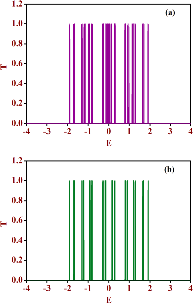
Figure 7: (Color online) Transmission characteristics of a $4$-th generation SPG-AB interferometer network for (a) $\Phi=0$ and (b) $\Phi=\Phi_{0}/4$. The other parameters are $\epsilon=0$, $t=1$, $N=5$, and the lead parameters are ${\mathcal{U}}_{L}=0$ and ${\mathcal{T}}_{L}=2$.

The upper panel shows the two-terminal transmission characteristics for a $4$-th generation network with $N=5$ in absence of any external magnetic flux. The poor conducting behavior of fractal networks in general is reflected in the transmission characteristics. There are of course, high, non-zero values of transmission coefficient for certain discrete values of energy $E$, which is at par with the existence of extended eigenstates in an otherwise fractal character of the energy spectrum of the system shown in Fig. 6. For a non-zero value of magnetic flux $\Phi=\Phi_{0}/4$ as shown in Fig. 7(b), the number of transmitting ‘zero-widhth windows’ of the system gets reduced compared to the zero flux case in (a), and finally for $\Phi=\Phi_{0}/2$, i.e., at half flux quantum the system becomes completely opaque to an incoming electron.

We have also examined the variation of the transmission coefficient with the magnetic flux $\Phi$ for fixed values of electron energy.

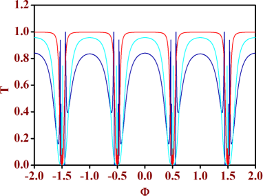
Figure 8: (Color online) Aharonov-Bohm oscillations for a $6$-th generation SPG-AB interferometer network at different values of electron energy, viz., $E=0.27840$ (red line), $E=1.29083$ (cyan line), and $E=1.91433$ (blue line). We have chosen $\epsilon=0$, $t=1$, $N=5$, and the lead parameters chosen are ${\mathcal{U}}_{L}=0$ and ${\mathcal{T}}_{L}=2$.

The transmission coefficient exhibits the typical oscillating behavior with the variation of the magnetic flux $\Phi$ known as the Aharonov-Bohm (AB) oscillation. One interesting feature is to observe that as we increase the value of the energy $E$, the AB oscillations get suppressed. In Fig. 8, we have plotted the AB oscillations in the transmittance of a sixth generation interferometer for three different values of energy, viz., $E=0.27840$ (red line), $E=1.29083$ (cyan line), and $E=1.91433$ (blue line). The suppression of AB oscillations is clearly visible.

V Conclusion

In conclusion, we have critically examined the electronic properties of a Sierpinski gasket geometry which is formed by arranging diamond shaped Aharonov-Bohm interferometers in appropriate order. The energy spectrum exhibits a rich structure comprising extended, staggered and edge-localized eigenfunctions. The number of such states depend on the number of quantum dots in each arm of the elementary diamond interferometer, and can populate the energy spectrum as densely as desired by the experimentalists. A constant magnetic field can be used to fine tune the locations of all these different classes of wave functions to initiate delicate switch on-switch off effects over arbitrarily small scales of energy. This could be useful from the perspective of a switching device that needed to operate over arbitrarily small scales of voltage. A magnetic flux equal to half-flux quantum leads to extreme localization of the wave function and Aharonov-Bohm cages.

- (1) Y. Aharonov and D. Bohm, Phys. Rev. B 115, 485 (1959).
- (2) S. Washburn and R. A. Webb, Adv. Phys. 35, 375 (1986).
- (3) M. Büttiker, Y. Imry, and M. Ya. Azbel, Phys. Rev. A 30, 1982 (1984).
- (4) R. Landauer and M. Büttiker, Phys. Rev. Lett. 54, 2049 (1985).
- (5) A. Levy Yeyati and M. Büttiker, Phys. Rev. B 52, R14360 (1995).
- (6) A. Yacoby, M. Heiblum, V. Umansky, H. Shtrikman, and D. Mahalu, Phys. Rev. Lett. 73, 3149 (1994).
- (7) A. Yacoby, M. Heiblum, D. Mahalu, and H. Shtrikman, Phys. Rev. Lett. 74, 4047 (1995).
- (8) M. Cassé, Z. D. Kvon, G. M. Gusev, E. B. Olshanetskii, L. V. Litvin, A. V. Plotnikov, D. K. Maude, and J. C. Portal, Phys. Rev. B 62, 2624 (2000).
- (9) B. Kubala and J. König, Phys. Rev. B 65, 245301 (2002).
- (10) T-S. Kim, S. Y. Cho, C. K. Kim, and C-M. Ryu, Phys. Rev. B 65, 245307 (2002).
- (11) K. Kobayashi, H. Aikawa, S. Katsumoto, and Y. Iye, Phys. Rev. Lett. 88, 256806 (2002).
- (12) A. Aharony, O. Entin-Wohlman, B. I. Halperin, and Y. Imry, Phys. Rev. B 66, 115311 (2002).
- (13) A. Aharony, O. Entin-Wohlman, and Y. Imry, Phys. Rev. Lett. 90, 156802 (2003).
- (14) A. Aharony, O. Entin-Wohlman, and Y. Imry, Turk. J. Phys. 27, 299 (2003).
- (15) C. Benjamin and A. M. Jayannavar, Phys. Rev. B 68, 085325 (2003).
- (16) V. Moldoveanu, M. Tolea, A. Aldea, and B. Tanatar, Phys. Rev. B 71, 125338 (2005).
- (17) H. Förster, S. Pilgram, and M. Büttiker, Phys. Rev. B 72, 075301 (2005).
- (18) A. Aharony and O. Entin-Wohlman, Phys. Rev. B 72, 073311 (2005).
- (19) F. E. Camino, W. Zhou, and V. J. Goldman, Phys. Rev. B 72, 155313 (2005).
- (20) A. Aharony, O. Entin-Wohlman, T. Otsuka, S. Katsumoto, H. Aikawa, and K. Kobayashi, Phys. Rev. B 73, 195329 (2006).
- (21) T. Kubo, Y. Tokura, T. Hatano, and S. Tarucha, Phys. Rev. B 74, 205310 (2006).
- (22) D. Urban and J. König, Phys. Rev. B 79, 165319 (2009).
- (23) T. Kubo, Y. Tokusain, and S. Tarucha, J. Phys. A: Math. Theo. 43, 354020 (2010).
- (24) M. Yamamoto, S. Takada, C. Bäuerle, K. Watanabe, A. D. Wieck, and S. Tarucha, Nature Nanotech. 7, 247 (2012).
- (25) A. Aharony, S. Takada, O. Entin-Wohlman, M. Yamamoto, and S. Tarucha, arXiv:1312.5177 [cond-mat.mes-hall] (2013).
- (26) J. S. Andrade Jr., H. J. Herrmann, R. F. S. Andrade, and L. R. da Silva, Phys. Rev. Lett. 94, 018702 (2005).
- (27) A. L. Cardoso, R. F. S. Andrade, and A. M. C. Souza, Phys. Rev. B 78, 214202 (2008).
- (28) I. N. Oliveira, F. A. B. F. de Moura, M. L. Lyra, J. S. Andrade Jr., and E. L. Albuquerque, Phys. Rev. E 79, 016104 (2009).
- (29) E. Domany, S. Alexander, D. Bensimon, and L. P. Kadanoff, Phys. Rev. B 28, 3110 (1983).
- (30) R. Rammal, J. Phys. (Paris) 45, 191 (1984); Phys. Rev. B 28, 4871 (1983).
- (31) J. R. Banavar, L. P. Kadanoff and A. M. M. Pruisken, Phys. Rev. B 31, 1388 (1985).
- (32) X. R. Wang, Phys. Rev. B 51, 9310 (1995).
- (33) J. M. Gordon, A. M. Goldman, and B. Whitehead, Phys. Rev. Lett. 59, 2311 (1987).
- (34) M. Li, Y. Liu, and Z-Q Zhang, Phys. Rev. B 61, 16193 (2000).
- (35) D. W. Cooley and D. R. Anderson, J. Opt. Soc. Am. B 24, A84 (2007).
- (36) Z. Gulácsi, A. Kampf, and D. Vollhardt, Phys. Rev. Lett. 99, 026404 (2007).
- (37) A. A. Lopes and R. G. Dias, Phys. Rev. B 84, 085124 (2011).
- (38) A. A. Lopes, B. A. Z. António, and R. G. Dias, Phys. Rev. B 89, 235418 (2014).
- (39) D. Bercioux, M. Governale, V. Cataudella, and V. M. Ramaglia, Phys. Rev. Lett. 93, 056802 (2004).
- (40) S. Sil, S. K. Maiti, and A. Chakrabarti, Phys. Rev. B 79, 193309 (2009).
- (41) J. L. Movilla and J. Planelles, Phys. Rev. B 84, 195110 (2011).
- (42) A. Aharony, Y. Tokura, G. Z. Cohen, O. Entin-Wohlman, and S. Katsumoto, Phys. Rev. B 84, 035323 (2011).
- (43) S. Matityahu, A. Aharony, O. Entin-Wohlman, and S. Katsumoto, Phys. Rev. B 87, 205438 (2013).
- (44) J. Vidal, R. Mosseri, and B. Douçot, Phys. Rev. Lett. 81, 5890 (1998).
- (45) J. Vidal, B. Douçot, R. Mosseri, and P. Butaud, Phys. Rev. Lett. 85, 3906 (2000).
- (46) J. Vidal, P. Butaud, B. Douçot, and R. Mosseri , Phys. Rev. B 64, 155306 (2001).
- (47) J. Vidal, G. Montambaux, and B. Douçot, Phys. Rev. B 62, R16294 (2000).
- (48) A. Chakrabarti, J. Phys.: Condens. Matter 8 10951 (1996).
- (49) B. Pal and A. Chakrabarti, Phys. Rev. B 85, 214203 (2012).
- (50) B. Pal and A. Chakrabarti, Eur. Phys. J. B 85, 307 (2012).
- (51) Y. Liu and K. A. Chao, Phys. Rev. B 34, 5247 (1986).